Model Adaptivity in Elasticity

THESIS FOR THE DEGREE OF LICENTIATE OF PHILOSOPHY

Model Adaptivity in Elasticity

DAVID HEINTZ

Department of Mathematical SciencesChalmers University of Technology and University of Gothenburg

Göteborg, Sweden 2008

Model Adaptivity in ElasticityDAVID HEINTZ

© DAVID HEINTZ, 2008

Thesis for Licentiate of PhilosophyNO 2008:37ISSN 1652-9715

Department of Mathematical SciencesChalmers University of Technology and University of GothenburgSE-412 96 GöteborgSwedenTelephone +46 (0)31–772 1000

Prepared with LATEXPrinted in Göteborg, Sweden 2008

Model Adaptivity in Elasticity

DAVID HEINTZ


Abstract

We consider model adaptivity in elasticity for dimensionally reduced forms, and shall treatdifferent conceptual approaches. The basic idea, however, is to adaptively refine, not onlythe computational mesh, but also the underlying mathematical formulation. The intention isthat the algorithm, provided with an hierarchy of models, should have the local complexitytailor-made for each problem, and thus become more efficient.

Reduced forms of the 3D-elasticity theory are typically obtained via simplified deforma-tion relations. A typical example is the Bernoulli and Timoshenko beam theories. We discussNavier’s equations of linear elasticity in a thin domain setting, and construct a model hierar-chy based on increasingly higher polynomials approximations through the thickness of thedomain, coupled with a Galerkin approach.

We suggest a finite element method for an extension of the Kirchhoff-Love plate equation,which includes the effects of membrane stresses. The stresses are obtained from the solutionof a plane-stress problem, and plays the role of underlying model. Since the modeling erroractually is a discretization error, it is not the same as the construction of a model hierarchy.

The aim has been to establish efficient solution procedures alongside accurate error con-trol. To succeed in this ambition, a posteriori error estimate are derived, which separate thediscretization and modeling errors. Frameworks for adaptive algorithms are suggested, andaccompanied by numerical results to exemplify their behavior.

Keywords: dimension reduction, model error, model adaptivity, a posteriori error

iii

List of Appended Papers

The licentiate thesis consists of an introductory text to subjects and methods, and new con-tributions based on the work in the following papers:

A D. Heintz, Model Adaptivity for Elasticity on Thin Domains, in Conference Proceed-ings, WCCM8/ECCOMAS 2008, Venice, Italy, 30 June–4 July 2008; Preprint 2008:34 (Blåserien), ISSN 1652-9715, Chalmers University of Technology and University of Gothen-burg

B P. Hansbo, D. Heintz and M. G. Larson, An Adaptive Finite Element Method forSecond Order Plate Theory, Preprint 2008:36 (Blå serien), ISSN 1652-9715, ChalmersUniversity of Technology and University of Gothenburg

Both papers are available at www.math.chalmers.se/Math/Research/Preprints/.

Paper B was prepared in collaboration with co-authors. The author of this thesis planned forand carried out the numerical simulations, and wrote the corresponding parts of the article.

v

Acknowledgments

The work in this thesis was funded by the Swedish Research Council, as part of the ongoingproject 621-2004-5147, by the name Model Adaptivity in Computational Mechanics.

Foremost, my gratitude goes to my supervisor, Professor Peter Hansbo: without his supportand encouragement, this thesis would not rest in your palms today. I also wish to thank myco-author Mats G. Larson.

I am much grateful to Thomas Ericsson. His expertise has guided me on numerous occa-sions (tends to Inf), and he is always in the mood for friendly conversations (as long as you“Don’t mention the element!”).

Niklas Ericsson has given me appreciated feedback—he taught me when I was an under-graduate, and continues doing so today.

I would like to thank the members of the Computational Mathematics group for provid-ing a pleasant working environment: especially Christoffer Cromvik, Karin Kraft and GöranStarius.

Last, but not least, I wish to address my colleagues at the former division of Computa-tional Technology: Thank you.

David HeintzGöteborg, November 2008

Contents

I Introduction 1

1 Model Adaptivity 31.1 Hierarchical Modeling in Elasticity . . . . . . . . . . . . . . . . . . . . . . . . . 41.2 The Finite Element Method . . . . . . . . . . . . . . . . . . . . . . . . . . . . . 6

1.2.1 Navier’s Equations of Elasticity . . . . . . . . . . . . . . . . . . . . . . . 71.2.2 Adaptivity . . . . . . . . . . . . . . . . . . . . . . . . . . . . . . . . . . . 9

1.3 Summary of Appended Papers . . . . . . . . . . . . . . . . . . . . . . . . . . . 141.4 Conclusions and Future Work . . . . . . . . . . . . . . . . . . . . . . . . . . . . 14

2 Implementation 17

II Papers 25

viii CONTENTS

Part I

Introduction

Chapter 1Model Adaptivity

We consider model adaptivity in computational mechanics, the focus being on hierarchicalmodeling within linear elasticity. However, let us begin by introducing the concept in gen-eral terms, and hence assume that we are studying a physical system, say, various potentialfields (gravitational, electrostatic, . . . ), stationary heat flow, or the displacements of a loadedelastic body. In order to answer the variety of questions which may arise, we try to describethe reality in terms of mathematical models, often in the guise of differential equations.

Since few physical problems are amenable to analytical methods, we need other meansto solve the mathematical model. In order to do so by using a computer, we must discretizethe continuous problem, and we choose to employ the finite element method (FEM), whichhas been closely intertwined with the solid mechanics community since the 1950s. We shallreturn to a discusson of FEM, particularly in the linear elasticity setting, in Section 1.2.

The discretized version constitutes a simplified problem, whose solution—which in ourcase is obtained via FEM—converges towards the continuous one, or at least becomes accu-rate enough, should the computational mesh just be sufficiently resolved. The meaning of“accurate enough” depends on the application at hand, and has turned into an importantresearch topic: solving the discretized problem is associated with a computational cost, interms of time and memory, and hence doing so without careful consideration could proveintractable. This was the advent of adaptive procedures in FEM, which basically are tech-niques for optimizing the underlying mesh. We want to distribute the degrees of freedomin such a way as to get high accuracy with respect to the computational cost. The a posteriorierror estimate is the cornerstone of such algorithms, providing local indicators to govern thedesign of the mesh, and, inherently, bringing error control.

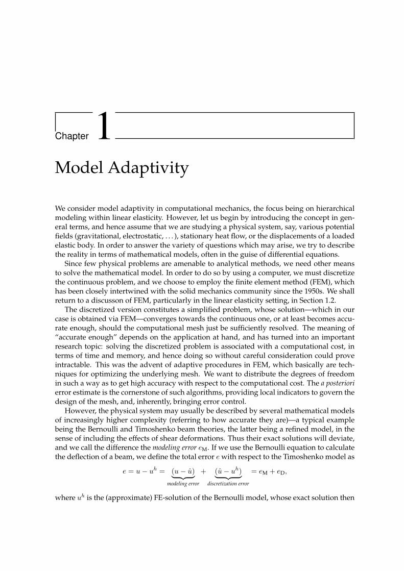
However, the physical system may usually be described by several mathematical modelsof increasingly higher complexity (referring to how accurate they are)—a typical examplebeing the Bernoulli and Timoshenko beam theories, the latter being a refined model, in thesense of including the effects of shear deformations. Thus their exact solutions will deviate,and we call the difference the modeling error eM. If we use the Bernoulli equation to calculatethe deflection of a beam, we define the total error e with respect to the Timoshenko model as

e = u− uh = (u− u)︸︷︷︸modeling error

+ (u− uh)︸︷︷︸discretization error

= eM + eD,

where uh is the (approximate) FE-solution of the Bernoulli model, whose exact solution then

4 CHAPTER 1. MODEL ADAPTIVITY

is denoted u. The conventional a posteriori error estimate measures the discretization erroreD (caused by not completely resolving the mesh). A schematic represention of the differenterror sources is shown in Figure 1. Note that even though eD → 0, implying uh → u, therestill remains a modeling error, which is not decreased by refining the mesh.

Suppose that we have a set of models to choose from, would it not be desirable also toadaptively refine the model? By starting at a simple model, and increase its complexity onlywhere it is necessary, we ought to get more efficient algorithms. Developing such techniques,in various settings, has become a new subject of research, which has intensified during thelast decade.

We have briefly introduced the concept of model error and model adaptivity, and willnow continue to discuss it, but concentrate on its application to elasticity.

beam deflection

approximate FE-soluttionof the Bernoulli equation

exact Bernoulli solution

exact Timoshenko solution

physical reality

discretization error

modeling error

total error with respectto the finer model

PSfrag replacements eD

eM e = eD + eM

FIGURE 1: Illustrating different error sources

1.1 Hierarchical Modeling in Elasticity

Boundary value problems (BVPs) encountered in engineering applications are often posedon thin domains, e.g., beams, plates or shells. The term thin then relates to the physical domainbeing much smaller in one direction. As an example consider the beam, which is dominatedby its extension in the axial direction. This may justify making simplifying assumptions onthe exact solution, effectively replacing the original problem with a lower-dimensional one.This is known as dimension reduction.

Lower-dimensional methods—as compared to the full elliptic 3D-BVPs—are more sus-ceptible to analytical techniques: sometimes it is even possible to derive exact solutions bymeans of Fourier series. Following the evolution of computers, these methods have gainedmore momentum, and are commonly used in today’s software. Some reasons for their pop-ularity are, firstly, the possible computational savings, and secondly, the fact that h-methodsin 3D FE-discretizations often require excessive mesh refinement, and could suffer from badconditioning (especially on thin domains), or exhibit so-called locking phenomena.

Lower-dimensional methods are usually advocated by being asymptotically exact, i.e., thedifference from the higher-dimensional model vanishes as the thickness (the extension in the

1.1. HIERARCHICAL MODELING IN ELASTICITY 5

thin direction) tends to zero. Nevertheless, in practice the thickness is prescribed, and hencewe inevitably incur a corresponding modeling error. But what should we do if our modelturns out not to be accurate enough?

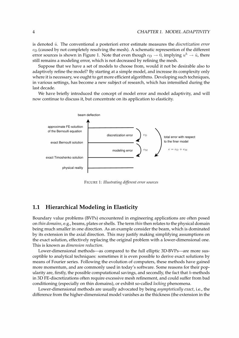
In the late 1980s and early 1990s the idea arose to embed classical models into a hierarchyof lower order models, the term hierarchic models being introduced by Szabo and Sahrmann,and the method further developed by Actis, Babuška and co-workers (see Schwab [26] forreferences). These hierarchies are typically constructed by imposing restrictions on the dis-placements of the 3D-formulations, say, by prescribing a polynomial expansion in the trans-verse direction. Consecutive models are then readily obtained by increasing the degree ofthe approximation. Once we have an available hierarchy, it could be used to solve the orig-inal formulation adaptively. The underlying model would not be uniform over the domain:the optimal model is tailor-made for each particular problem (illustrated in Figure 2).

0 0.2 0.4 0.6 0.8 1 −0.4

−0.3

−0.2

−0.1

0

0.1

0.2

0.3

1 2 3 4 5 6 7 8 9 1011

PSfrag replacements

x1

x2

poly

nom

ialdegre

e

FIGURE 2: FE-solution for fixed loaded beam by means of model adaptivity; the solution of the correspondingBernoulli beam equation is seen in solid gray (Paper I)

The goal of adaptive algorithms is to reduce the total error within a prescribed tolerance.The notion of the total error being divided into two distinct parts, namely the discretizationand modeling errors, means that we, in each stage of our computation, need to determinewhether to refine the model or enrich the finite dimensional subspace. The decision ought tobring forward an equidistribution of the total error, which in turn requires any a posteriorierror analysis to include two estimates, one for each error type. Our primary concern thusbecomes to decompose the error into these distinct parts.

The early approaches assumed the discretization error to be negligible, so that the mod-eling error, more or less, constituted the total error itself. The error estimates were refined tomeasure the error in global norms (energy norm), and in recent years, extended to encom-pass upper and lower bounds in linear functionals of the solution. We will return to discusssuch techniques in Sections 1.2.2 and 1.2.2.


1.2 The Finite Element Method

FEM is a numerical technique for solving general partial differential equations (PDEs) overcomplex geometries. Instead of approximating the differential equation directly, which a tra-ditional finite difference method (FDM) would do, it uses integrated forms, correspondingto alternative descriptions of the physical problem.

FEM is closely related to global balance laws, e.g., minimization of the potential energy andthe balance of virtual work. To exemplify the latter, we consider the stationary 1D heat con-duction in a bar, which is described by the following model problem (see [11, Section 6.2.1]for details)

−(ku′)′ = f, 0 < x < 1, (1)

where k > 0 is the heat conductivity, −ku′ is the heat flux, and f is an external heat source.Assuming homogeneous Dirichlet boundary conditions, u(0) = u(1) = 0, we multiply (1)by a function v, such that v(0) = v(1) = 0, and integrate over the domain∫ 1

0−(ku′)′v dx =

∫ 1

0fv dx, (2)

which, following integration by parts, leads to the weak form∫ 1

0ku′v′ dx =

∫ 1

0fv dx. (3)

We call the functions u and v the trial and test functions, and say that we have tested (1) withv. If one tests by a sufficiently large number of functions v, we expect the integrated form(2) to actually satisfy (1) pointwise (the virtual work principle becomes equivalent with theenergy conservation law and Fourier’s law underlying (1)). Note that (3) imposes fewer re-strictions on u than a classical solution of (1) does. The weak solution, e.g, is not required tobe twice differentiable, the integrals should just exist. This is an important point: it is easierto generate approximate solutions of less regularity (consequently FEM produces approxi-mate solutions of (3) rather than (1)).

Galerkin’s method is based on seeking an approximate solution in a finite-dimensionalspace, spanned by a set of basis functions, which are easy to differentiate and integrate. Thiscould be piecewise linear continuous functions ϕi = ϕi(x) with local support (the basic formof a FEM). If the FE-solution is written

uh(x) =n∑i=1

uiϕi(x), (4)

then Galerkin suggested (3) to hold for all test functions of the same form. To ensure this, theequation is tested against each ϕi separately (then it will be satisfied for an arbitrary linearcombination of the basis functions). We get a linear system of equations to be solved for thecoefficients ui of (4) using a computer.

Galerkin’s method can be described as a projection method, where the solution is projectedonto a subspace, spanned by a set of basis functions. These functions are not necessarily lin-ear, but can be polynomials of higher order, or even trigonometric functions (so-called spec-tral methods). We can make a discontinuous ansatz for the FE-solution as well. The method

1.2. THE FINITE ELEMENT METHOD 7

can also be formulated using different functions in the test and trial spaces, which is knownas a Petrov-Galerkin method.

FEM has a solid mathematical foundation, see, e.g., [12] and [7], which is a strength, sinceit provides tools for deriving analytical error estimates, that, in turn, allow us to improveon our approximate solutions. FEM has typically been the natural choice for applications insolid mechanics. FDM, somewhat easier to implement than FEM (at least for simpler modelproblems on rectangular domains), is more common within the field of computational fluiddynamics. Here one otherwise tends to employ lower-order finite volume methods.

We now turn to the equations of linear elasticity, and introduce the corresponding strong,weak and FE-formulations. Solving Navier’s equations—or, in some sense, avoiding it!—has been an integral part of this thesis. In Paper I we treat a reduced form on thin domains,whereas Paper II deals with second order effects for plate theory. The terminology of finiteelements is closely intertwined with elasticity, e.g., the linear system of equations arising inFEM, Su = f , usually calls S and f the stiffness matrix and load vector, respectively, regardlessof the actual application. How to assemble FE-matrices in an efficient manner is discussedin Chapter 2.

1.2.1 Navier’s Equations of Elasticity

Consider a convex polygonal domain Ω ⊂ R2, representing a deformable medium subjectedto external loads. These include body forces f and surface tractions g, causing deformationsof the material, which we describe by the following model problem: Find the displacementfield u = (u1, u2) and the symmetric stress tensor σ = (σij)2

i,j=1, such that

σ(u) = λ div(u) I + 2µε(u) in Ω (5)−div(σ) = f in Ω (6)

u = 0 on ∂ΩD

σ · n = g on ∂ΩN

where ∂Ω = ∂ΩD ∪ ∂ΩN is a partitioned boundary of Ω. Let the Lamé coefficients

λ =Eν

(1 + ν)(1− 2ν), µ =

E

2(1 + ν), (7)

with E and ν being Young’s modulus and Poisson’s ratio, respectively. Furthermore, I is theidentity tensor, n denotes the outward unit normal to ∂ΩN, and the strain tensor is

ε(u) = 12

(∇u+∇uT).The vector-valued tensor divergence is

div(σ) =( 2∑j=1

∂σij∂xj

)2

i=1

,

representing the internal forces of the equilibrium equation (6). This formulation assumes aconstitutive relation corresponding to linear isotropic elasticity (the material properties arethe same in all directions), with stresses and strains related by

σv =

σ11

σ22

σ12

=

D11 D12 D13

D21 D22 D23

D31 D32 D33

ε11

ε22

ε12

= D(λ, µ)εv,


referred to as Hooke’s generalized law. Should the material be homogeneous, D becomes in-dependent of position.

In order to pose a weak formulation we introduce the function space

V =v : v ∈ H2(Ω), v|∂ΩD= 0

,

and state: Find u ∈ V × V such that

a(u,v) = L(v), ∀v ∈ V × V, (8)

where the bilinear form

a(u,v) =∫

Ωσ(u) : ε(v) dx (9)

is the integrated tensor contraction

σ : ε def=2∑

i,j=1

σijεij ,

and the linear functional

L(v) = (f ,v) + (g,v)∂ΩN =∫

Ωf · v dx+

∫∂ΩN

g · v ds. (10)

We usually interpret (8) as a balance between the internal (9) and external (10) “virtual work”(with the test functions v being “virtual displacements”).

For the numerical approximation of (8), we shall need a discrete counterpart, and as suchestablish a finite element method. To simplify its formulation we define the kinematic rela-tion

εv(u) =

∂∂x1

00 ∂

∂x2

∂∂x2

∂∂x1

[u1

u2

]= ∇u,

and specify the constitutive matrix

D =

λ+ 2µ λ 0λ λ+ 2µ 00 0 µ

,for the purpose of rewriting the bilinear form as

a(u,v) =∫

Ωεv(u)TDεv(v) dx,

which facilitates implementation. We introduce a partition Th of Ω, dividing the domain intoNel elements. More precisely, we let Th = K be a set of triangles K, such that

Ω =⋃K∈Th

K,


with the element vertices referred to as the nodes xi, i = 1, 2, . . . , Nno, of the triangulation.The intersection of any two triangles is either empty, a node, or a common edge, and no nodelies in the interior of an edge (there are no hanging nodes). The function

hK = diam(K) = maxy1,y2∈K

(‖y1 − y2‖2), ∀K ∈ Th,

represents the local mesh size. Moreover, Eh = E denotes the set of element edges, whichwe split into two disjoint subsets, Eh = EI ∪ EB , namely the sets of interior and boundaryedges, respectively. The partition is associated with a function space

Vh = v ∈ C(Ω) : v is linear on K for each K ∈ Th, v|∂ΩD= 0 , (11)

consisting of continuous, piecewise linear functions, that vanish on the Dirichlet boundary.A function v ∈ Vh is uniquely determined by its values at xi, together with the set of shapefunctions

ϕjNnoj=1 ⊂ Vh, ϕj(xi) := δj(xi),

which constitute a nodal basis for (11). It then follows that any v ∈ Vh can be expressed as alinear combination

v =Nno∑j=1

vjϕj(x), (12)

where vj = v(xj) represents the j:th nodal value of v. We make an ansatz for a FE-solutionof this type (12), and hence our FE-formulation of (8) becomes: Find uh ∈ Vh × Vh such that

a(uh,v) = L(v), ∀v ∈ Vh × Vh, (13)

whose solution usually is written on the standard form

uh =[ϕ1 0 ϕ2 0 . . .0 ϕ1 0 ϕ2 . . .

]u1

1

u12

u21

u22...

= ϕu,

associating odd and even elements of u with displacements in x1 and x2, respectively. Sincetesting against all v ∈ Vh × Vh reduces to testing against ϕjNno

j=1, and εv(uh) = ∇ϕu = Bu,(13) corresponds to solving∫

ΩBTDB dxu =

∫ΩϕTf dx+

∫∂ΩN

ϕTg ds, (14)

i.e., the matrix problem Su = f , making (14) a suitable starting point for FE-implementation.

1.2.2 Adaptivity

The goal in FE-analysis, from a practical point of view, is to utilize the available computingresources in an optimal way, usually adhering to either of two principles:


• obtain the prescribed accuracy TOL at minimal amount of work;

• obtain the best accuracy for a prescribed amount of work.

In order to achieve this aim, the traditional approach is by means of automatic mesh adap-tion, based on local error indicators. These are functions of the FE-solution, and presumablymeasure the local roughness of the continuous solution. The overall process involves somedistinct steps:

i) a choice of norm in which the error is defined (different problems may call for differentnorms);

ii) a posteriori error estimates with respect to the chosen norm, in terms of known quanti-ties, i.e., the data and the FE-solution (which provide information about the continuousproblem);

iii) local error indicators extracted from the (global) a posteriori error estimates;

iv) a strategy for changing the mesh characteristics (the mesh size and/or the polynomialinterpolation) to reduce the error in an (nearly) optimal way.

In the following we deal with questions i)-ii) in some detail. The discussion will not be com-prehensive, but focuses on exemplifying the techniques employed in this thesis: 1) residual-based energy norm control (used in Paper I); and 2) goal-oriented adaptivity (Paper II).

For the sake of simplicity, we let Poisson’s equation serve as model problem, representingthe linear elliptic PDE. Let us adopt parts of the notation from Section 1.2.1, and hence posethe continuous problem: Find u such that

Au := −∇ · (k∇u) = f, in Ω, (15)u = 0, on ∂ΩD,

n · k∇u = g, on ∂ΩN,

where we assume the coefficient k = k(x) to be smooth, whereas f ∈ L2(Ω) and g ∈ L2(∂ΩN)are data to the problem.

Residual-Based Error Estimates

The main idea—as opposed to solving local problems or using stress projections—is to sub-stitute the FE-solution into the PDE: since uh is an approximation, it does not satisfy (15)exactly, and this hopefully provides useful information about the error e = u− uh.

The weak form of the model problem is: Find u ∈ V such that

a(u, v) = L(v), ∀v ∈ V, (16)

where the bilinear form a(·, ·) and the linear functional L(·) are

a(u, v) =∫

Ωk∇u · ∇v dx, L(v) =

∫Ωfv dx+

∫∂ΩN

gv ds.

The corresponding FE-formulation becomes: Find uh ∈ Vh such that

a(uh, v) = L(v), ∀v ∈ Vh, (17)


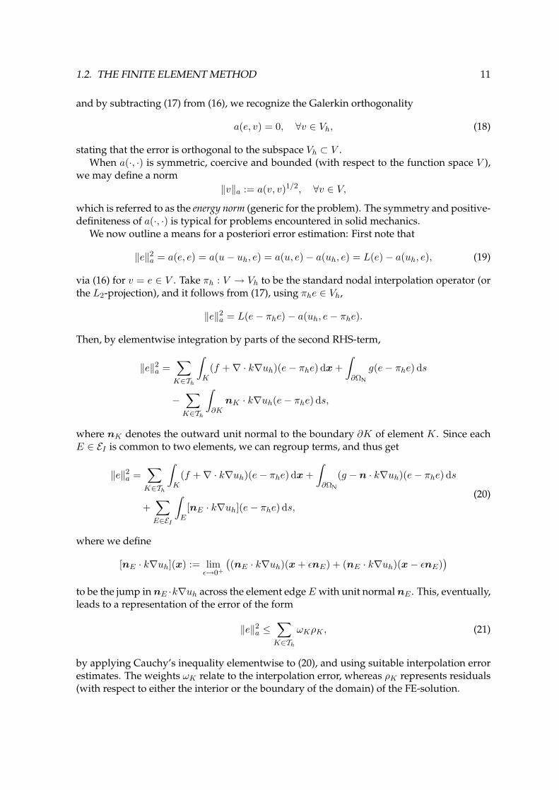
and by subtracting (17) from (16), we recognize the Galerkin orthogonality

a(e, v) = 0, ∀v ∈ Vh, (18)

stating that the error is orthogonal to the subspace Vh ⊂ V .When a(·, ·) is symmetric, coercive and bounded (with respect to the function space V ),

we may define a norm‖v‖a := a(v, v)1/2, ∀v ∈ V,

which is referred to as the energy norm (generic for the problem). The symmetry and positive-definiteness of a(·, ·) is typical for problems encountered in solid mechanics.

We now outline a means for a posteriori error estimation: First note that

‖e‖2a = a(e, e) = a(u− uh, e) = a(u, e)− a(uh, e) = L(e)− a(uh, e), (19)

via (16) for v = e ∈ V . Take πh : V → Vh to be the standard nodal interpolation operator (orthe L2-projection), and it follows from (17), using πhe ∈ Vh,

‖e‖2a = L(e− πhe)− a(uh, e− πhe).

Then, by elementwise integration by parts of the second RHS-term,

‖e‖2a =∑K∈Th

∫K

(f +∇ · k∇uh)(e− πhe) dx+∫∂ΩN

g(e− πhe) ds

−∑K∈Th

∫∂KnK · k∇uh(e− πhe) ds,

where nK denotes the outward unit normal to the boundary ∂K of element K. Since eachE ∈ EI is common to two elements, we can regroup terms, and thus get

‖e‖2a =∑K∈Th

∫K

(f +∇ · k∇uh)(e− πhe) dx+∫∂ΩN

(g − n · k∇uh)(e− πhe) ds

+∑E∈EI

∫E

[nE · k∇uh](e− πhe) ds,(20)

where we define

[nE · k∇uh](x) := limε→0+

((nE · k∇uh)(x+ εnE) + (nE · k∇uh)(x− εnE)

)to be the jump innE ·k∇uh across the element edgeE with unit normalnE . This, eventually,leads to a representation of the error of the form

‖e‖2a ≤∑K∈Th

ωKρK , (21)

by applying Cauchy’s inequality elementwise to (20), and using suitable interpolation errorestimates. The weights ωK relate to the interpolation error, whereas ρK represents residuals(with respect to either the interior or the boundary of the domain) of the FE-solution.


(21) is an a posteriori error estimate, i.e., an estimate in terms of the computed solutionand data, which constitutes an upper bound of the error. However, being based on Cauchy’sinequality, it may not be sharp. A viable alternative comes by solving an auxiliary problemon a refined mesh. The enhanced discrete solution u is then interpolated onto the primalmesh, and the difference provides information about the error. This technique was used inPaper I for Navier’s equations of elasticity, and it is also shown how local error indicatorscan be extracted.

Approximating u on a refined mesh clearly is expensive—hence we comment on the op-tion of solving local problems (see Verfürth [32, Chapter 1.3] for details). It is usually cheaperto solve a set of smaller problems, but possibly less straightforward to implement. Dirichletproblems can be constructed by raising the degree of the polynomial approximation. Let usexemplify by going from linear to quadratic: The boundary values are then inherited fromuh, providing an extra degree of freedom on each element. Alas, to obtain reliable estimatesfor u, one often needs to consider patches of elements (say all elements including a node, toyield additional degrees of freedom), which requires extra work. For Neumann problems,on the other hand, we have to equilibrate an approximation of the flux k∇u, to keep the es-timates from degrading (since there are no Dirichlet boundary conditions). The use of localNeumann problems for error estimation in hierarchical models have been pursued by Steinand Ohnimus in a series of papers [27, 28, 29].

Goal-Oriented Adaptivity

The traditional approach to adaptivity is to estimate the error in energy norm or the globalL2-norm. However, more often than not, we are rather interested in controlling the error oflocal physical quantities, like the maximum deflection of a plate subjected to external loads.

In order to assess this error we shall use duality techniques, which essentially means thatwe multiply the residuals by certain weights, namely the solution of a so-called dual problem(hence the approach is known as the dual-weighted residual method—or the DWR-method forshort). To show this we begin by introducing the continuous dual (adjoint) problem:

ATz = j, (22)

where the dual operator AT is defined by

(ATz, ψ) = (z,Aψ). (23)

We can show that

(e, j)(22)= (e,ATz)

(23)= (Ae, z) = (f −Auh, z) (18)

= (f −Auh, z − πhz), (24)

using the Galerkin orthogonality for v = πhz ∈ Vh. Now, as compared to (19), we are free tochoose the data j according to the quantity we wish to control adaptively—if j is taken as anapproximate Dirac delta function, the LHS of (24) reduces to the error in the correspondingpoint (cf. Paper II).

Example. In order to concretize (24), we return to Poisson’s equation, and test (15) against a


function z:∫Ω−∇ · (k∇u)z dx =

∫Ωk∇u · ∇z dx−

∫∂ΩN

n · (k∇u)z ds

=∫

Ω−∇ · (k∇z)udx−

∫∂ΩN

(n · (k∇u)z − n · (k∇z)u) ds,

using integration by parts twice. Taking the Neumann boundary conditions into account (uis prescribed on the Dirichlet boundary), this indicates that the dual problem should be

ATz = −∇ · (k∇z) = j1, in Ω,z = 0, on ∂ΩD,

n · k∇z = j2, on ∂ΩN,

i.e., A = AT is a self-adjoint operator. We first note that

(e,ATz) =∫

Ω−∇ · (k∇z)e dx =

∫Ωk∇z · ∇e dx−

∫∂ΩN

j2e ds,

and then, via (24) for data j1 and j2,

(e, j1) + (e, j2)∂ΩN =∫

Ωk∇z · ∇e dx = a(e, z)

(18)= a(e, z)− a(e, πhz)

= a(u− uh, z − πhz) = a(u, z − πhz)− a(uh, z − πhz).

By expressing the former a(·, ·)-functional in terms of data,

(e, j1) + (e, j2)∂ΩN = (f, z − πhz) + (g, z − πhz)∂ΩN − a(uh, z − πhz),

allowing us to control functionals of the error both inside the domain and on the Neumannboundary.

We emphasize that the dual problem cannot be solved exactly, at least not in general, andthus has to be approximated. So a tempting idea, from a practical point of view, would be toreuse the primal mesh: Find zh ∈ Vh such that

a(v, zh) = (j, v) = J(v), ∀v ∈ Vh, (25)

but this does not work. The reason why is that the Galerkin orthogonality leads to the trivialerror representation

J(e)(24)= (f −Auh, zh − πhz) = 0,

since zh and πhzh will coincide. Hence we typically need the dual approximation to be moreaccurate than the FE-solution—the approach in Paper II was to solve the dual plate andplane stress problems with respect to enriched function spaces. This may be straightforward,but also computationally demanding. Focusing on evaluating the suggested FEM, we didnot pursue any alternatives, e.g., by post-processing a solution of (25) to get an estimate ofz−πhz (we refer to Larsson et al. [15] for working strategies). The procedure is merited onlyfor illustrating the convergence of the error estimator for various meshes.


If the data of the dual problem is a function of the error itself, i.e., j = j(e), we somehowhave to approximate the error, besides estimating z − πhz, which obviously becomes time-consuming. In Paper II this was not necessary for the dual plate problem, where j = j(uh)(a pointwise displacement), but the dual plane stress problem required an approximation u(which was retrieved alongside z at a small cost). If we want to control the error in normsother than the energy norm, or in a linear functional of the error, the information inevitablycomes at a price.

This short review did not encompass the (interesting) non-linear variational formulation,as this was outside the scope of Paper II, which then calls for a linearization of the continu-ous dual problem. The interested reader is referred to Larsson [14, Section 2] and Bangerthand Rannacher [4].

Using duality arguments in a posteriori error estimation was introduced during the early1990s, in works by Eriksson et al. [10] among others. It was later developed into the DWR-method by Becker and Rannacher [5]. Quantitative error control by computational meansakin to the DWR-method, in the context of model adaptivity, has been seen in, e.g., Oden etal. [18, 20, 31] (solid/fluid mechanics applications and heterogeneous materials) and Braackand Ern [6] (Poisson’s equation, convection-diffusion-reaction equations). Recent work inmodel and goal adaptivity, within the field of multiscale modeling, includes Oden et al. [19].

1.3 Summary of Appended Papers

In Paper I, Model Adaptivity for Elasticity on Thin Domains, we consider Navier’s equations intwo spatial dimensions, with the main idea of constructing a model hierarchy to facilitate thesolution procedure. Being based on increasingly higher polynomial expansions through thethickness of the domain (coupled with a Galerkin approach), the suggested hierarchy seemslike a natural extension of the Bernoulli and Timoshenko beam theories. Energy norm errorestimates are outlined, which motivate uncoupling of the discretization and modeling errors,thereby providing local error indicators. We introduce an adaptive algorithm, concurrentlyrefining mesh and model, and evaluate its behavior. The numerical results indicate sharperror control.

In Paper II, An Adaptive Finite Element Method for Second Order Plate Theory, the fourth-order Kirchhoff-Love model is supplemented by a second-order term to include the effectsof membrane stresses. The plate is approximated by piecewise continuous second degreepolynomials (having discontinuous derivatives), whereas the in-plane deformations (whichare not used explicitly) are represented by a constant-strain element. We derive an a posteri-ori error estimate, separating the bending and membrane effects (the stresses thereby appearas a modeling error), for controlling a linear functional of the error. A goal-oriented adaptivealgorithm is proposed, and evaluated with respect to the maximum plate deflection, undervarious loading conditions. Effectivity indices close to unity suggest sharp error control.

1.4 Conclusions and Future Work

We consider model adaptivity in linear elasticity for dimensionally reduced forms: Paper Idiscusses a thin domain setting, whereas Paper II treats an extension of the Kirchhoff-Love

1.4. CONCLUSIONS AND FUTURE WORK 15

plate equation. The aim has been to establish efficient solution procedures—including accu-rate error control—by adapting, not the discretization of the computational domain alone,but also the underlying model, i.e., the mathematical formulation of the physical problem.To change the model we need an hierarchy (the approach in Paper II is somewhat different)to choose from, and a means to indicate when and where a substitution should take place.This means that the complexity of the model varies over the domain, just as the local meshsize does, to ensure that the total error is efficiently minimized.

In Paper I we constructed a model hierarchy, which was used to solve a small set of testproblems, and it managed to do so accurately. The adaptive algorithm was not thoroughlytested, though, but the approach seems promising. For the cantilever beam (square domain)it was actually more efficient than the Zienkiewicz-Zhu method used in [2], where bilinearelements were applied in a standard setting (without a thin domain approach). We empha-size this to be in terms of degrees of freedom, as the computational costs were not compared.

Paper II has the more flexible approach of goal-adaptive error control. The error esti-mator was efficient throughout the iterative procedures, which is important for problems inengineering analysis (the mesh size does not tend to zero in practice).

The extension of the existing model hierarchy in Paper I is the goal for future work, i.e.,to introduce the Bernoulli and Timoshenko beam theories as simpler models. The elementsshould be altered to adopt hierarchical basis functions for improved numerical stability. Thiscould be done by following Vogelius and Babuška [33], and employ Legendre polynomialsinstead. The error estimates may be sharpened, e.g., to account for geometrical anisotropy.

However, another and more challenging problem, is to apply the thin domain approach ina higher dimension. The 3D-elasticity formulation could then be reduced by using increas-ingly higher polynomial expansions through the thickness. The idea is by no means novel,being the subject of study in numerous articles, e.g., in Babuška and Schwab [3], Ainsworth[1], and Repin et al. [25]. They derived residual-based estimates in energy norm, whereasVemaganti [30] used duality-based techniques to control a continuous linear functional of theerror. Our approach would deviate by relying on the method in Paper II, for the Kirchhoff-Love model, supplemented by the Reissner-Mindlin plate. The former is to be regarded asthe basic model, and the latter is more complex, since it introduces additional rotational de-grees of freedom. The FEM presented by Hansbo and Larson [13], based on discontinuousP 1-approximations for the rotations, and continuous piecewise quadratic polynomials forthe transverse displacements, may serve as a starting point. Additional ideas for bridgingthe Reissner-Mindlin plate with a thin domain hierarchy stem from Nitsche’s method [17].The focus shall be on a goal-adaptive approach, where solving the adjoint problems in cost-efficient manner will be desirable.

Chapter 2Implementation

We shall provide a few hints on how to implement FE-algorithms in an efficient manner. Theintention is not to be comprehensive, as getting good performance out of a computer systemis a complex task, but focuses on some common tools, which were used for writing the codesunderlying the numerical simulations of this thesis.

When writing scientific software there are several things to bear in mind, and depending onits use, the order of priority will be different. However, the basic ubiquitous principles are:

• correctness,

• numerical stability,

• flexibility,

• efficiency.

The first point needs no further explanation—if the program is not correct, it will not do thework. If the algorithm is not stable, one cannot trust the results1 (unless they are thoroughlytested). It must be flexible to be useful—making small changes should come easy. Assuminga correct implementation of a numerically stable algorithm, then we can turn to optimizationin terms of speed and memory2. A nice textbook for implementing scientific software is [24].

Experience set aside—hard lessons have taught us that FE-implementations are not free frombugs!—we turn our attention to efficiency. In particular, we concentrate on single-core CPUs(although the techniques we exemplify could be parallelized), and MATLAB [22] becomesour choice for a programming environment. The reason why is closely related to flexibil-ity: MATLAB is based on the abstraction of matrices, using a consistent set of internal datastructures, allowing for relatively effortless FE-implementation. The builtin visualization ca-pabilities are powerful enough for most purposes. Hence it suits the needs of research codeswell, where the primary objective is the evaluation of algorithms, and hard time spent onoptimization is less worthwile (the final code may only be executed a few times). An alter-native to MATLAB, which has the benefit of being distributed under an open-source license,

1Thus means for estimating the error of approximations are essential, error control being an integral part ofadaptive FE-algorithms, just as important, if not more, as efficiency is.

2Memory is crucial, since an algorithm requiring more memory than the machine has, simply will not run.

18 CHAPTER 2. IMPLEMENTATION

is Python. Production codes, that run on a daily basis, have different demands, and usuallyrely on compiled languages, say, Fortran or C/C++.

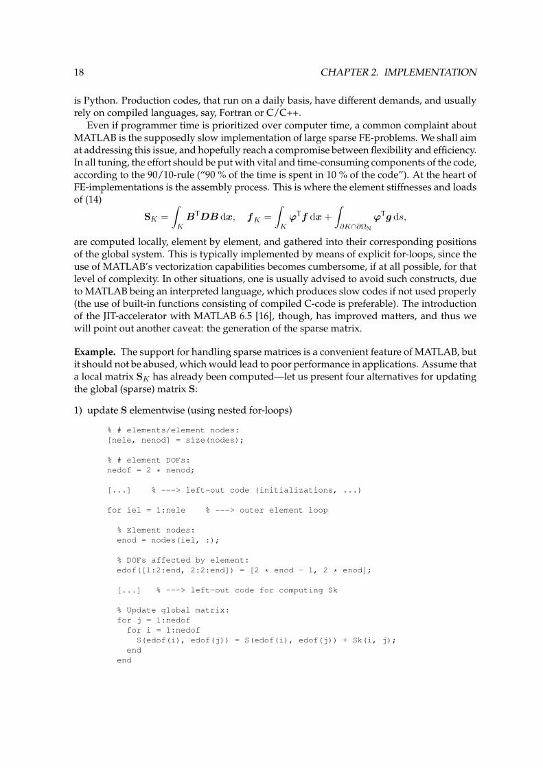
Even if programmer time is prioritized over computer time, a common complaint aboutMATLAB is the supposedly slow implementation of large sparse FE-problems. We shall aimat addressing this issue, and hopefully reach a compromise between flexibility and efficiency.In all tuning, the effort should be put with vital and time-consuming components of the code,according to the 90/10-rule (“90 % of the time is spent in 10 % of the code”). At the heart ofFE-implementations is the assembly process. This is where the element stiffnesses and loadsof (14)

SK =∫KBTDB dx, fK =

∫KϕTf dx+

∫∂K∩∂ΩN

ϕTg ds,

are computed locally, element by element, and gathered into their corresponding positionsof the global system. This is typically implemented by means of explicit for-loops, since theuse of MATLAB’s vectorization capabilities becomes cumbersome, if at all possible, for thatlevel of complexity. In other situations, one is usually advised to avoid such constructs, dueto MATLAB being an interpreted language, which produces slow codes if not used properly(the use of built-in functions consisting of compiled C-code is preferable). The introductionof the JIT-accelerator with MATLAB 6.5 [16], though, has improved matters, and thus wewill point out another caveat: the generation of the sparse matrix.

Example. The support for handling sparse matrices is a convenient feature of MATLAB, butit should not be abused, which would lead to poor performance in applications. Assume thata local matrix SK has already been computed—let us present four alternatives for updatingthe global (sparse) matrix S:

1) update S elementwise (using nested for-loops)

% # elements/element nodes:[nele, nenod] = size(nodes);

% # element DOFs:nedof = 2 * nenod;

[...] % ---> left-out code (initializations, ...)

for iel = 1:nele % ---> outer element loop

% Element nodes:enod = nodes(iel, :);

% DOFs affected by element:edof([1:2:end, 2:2:end]) = [2 * enod - 1, 2 * enod];

[...] % ---> left-out code for computing Sk

% Update global matrix:for j = 1:nedoffor i = 1:nedofS(edof(i), edof(j)) = S(edof(i), edof(j)) + Sk(i, j);

endend

19

end

2) update S “matrixwise” (vectorizing loops)

% Update global matrix:S(edof, edof) = S(edof, edof) + Sk;

3) generate S using index vectors

% # DOFs in mesh:ndof = 2 * length(xnod);

% # local matrix elements:nn = (2 * nenod)^2;

% Index vectors:row = zeros(nn * nele, 1);col = row;val = row;up = 0;

[...]

for iel = 1:nele

[...]

% Update index vectors:XM = edof(:, ones(1, nedof));YM = XM’;lo = up + 1;up = up + nn;row(lo:up) = XM(:);col(lo:up) = YM(:);val(lo:up) = Sk(:);

end

% Construct sparse stiffness matrix:S = sparse(row, col, val, ndof, ndof);

4) use faster sparse2 function

% Construct sparse stiffness matrix:S = sparse2(row, col, val, ndof, ndof);

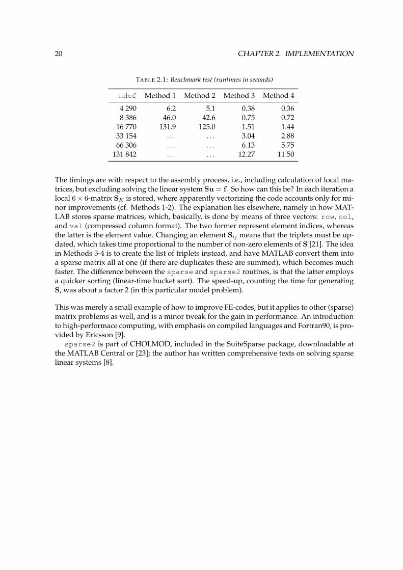
We have only included necessary parts of the assembly routine (dots within brackets meansthat code has been omitted): nodes is a topology matrix, where the i:th row holds the globalnode numbers on elementKi, and xnod stores the x1-coordinates of all nodes. A benchmarktest3, solving the plain strain formulation of Paper I (cantilever beam with t = 1) using lineartriangles, reveals significant differences in performance:

3Setup (hardware/OS/version): AMD Athlon™ 64 3200+ (single core CPU with 512 kB L2-cache) and 1 024MB RAM; running RHEL 4.6 and MATLAB 2007b.

20 CHAPTER 2. IMPLEMENTATION

TABLE 2.1: Benchmark test (runtimes in seconds)

ndof Method 1 Method 2 Method 3 Method 4

4 290 6.2 5.1 0.38 0.368 386 46.0 42.6 0.75 0.72

16 770 131.9 125.0 1.51 1.4433 154 . . . . . . 3.04 2.8866 306 . . . . . . 6.13 5.75

131 842 . . . . . . 12.27 11.50

The timings are with respect to the assembly process, i.e., including calculation of local ma-trices, but excluding solving the linear system Su = f . So how can this be? In each iteration alocal 6× 6-matrix SK is stored, where apparently vectorizing the code accounts only for mi-nor improvements (cf. Methods 1-2). The explanation lies elsewhere, namely in how MAT-LAB stores sparse matrices, which, basically, is done by means of three vectors: row, col,and val (compressed column format). The two former represent element indices, whereasthe latter is the element value. Changing an element Sij means that the triplets must be up-dated, which takes time proportional to the number of non-zero elements of S [21]. The ideain Methods 3-4 is to create the list of triplets instead, and have MATLAB convert them intoa sparse matrix all at one (if there are duplicates these are summed), which becomes muchfaster. The difference between the sparse and sparse2 routines, is that the latter employsa quicker sorting (linear-time bucket sort). The speed-up, counting the time for generatingS, was about a factor 2 (in this particular model problem).

This was merely a small example of how to improve FE-codes, but it applies to other (sparse)matrix problems as well, and is a minor tweak for the gain in performance. An introductionto high-performace computing, with emphasis on compiled languages and Fortran90, is pro-vided by Ericsson [9].

sparse2 is part of CHOLMOD, included in the SuiteSparse package, downloadable atthe MATLAB Central or [23]; the author has written comprehensive texts on solving sparselinear systems [8].

Bibliography

[1] M. Ainsworth, A posteriori error estimation for fully discrete hierarchic models of ellipticboundary problems on thin domains, Numerische Mathematik 80 (1998), 325–362.

[2] M. Ainsworth, J. Z. Zhu, A. W. Craig, and O. C. Zienkiewicz, Analysis of the Zienkiewicz-Zhu a posteriori error estimator in the finite element method, International Journal for Nu-merical Methods in Engineering 28 (1989), 2161–2174.

[3] I. Babuška and C. Schwab, A posteriori error estimation for hierarchic models of ellipticboundary value problems on thin domains, SIAM Journal on Numerical Analysis 33 (1996),no. 1, 221–246.

[4] W. Bangerth and R. Rannacher, Adaptive Finite Element Methods for Differential Equations,Birkhäuser Verlag, 2003.

[5] R. Becker and R. Rannacher, An optimal control approach to a posteriori error estimation infinite element methods, Acta Numerica 10 (2001), 1–102.

[6] M. Braack and A. Ern, A posteriori control of modeling errors and discretization errors, SIAM:Multiscale Modeling and Simulation 1 (2003), no. 2, 221–238.

[7] S.C. Brenner and L.R. Scott, The Mathematical Theory of Finite Element Methods, 2:nd ed.,Springer-Verlag, 2002.

[8] T.A. Davis, Direct Methods for Sparse Linear Systems, SIAM: Fundamentals of Algorithms,2006.

[9] T. Ericsson, Performance engineering, http://www.math.chalmers.se/~thomas/PDC/springer.pdf.

[10] K. Eriksson, D. Estep, P. Hansbo, and C. Johnson, Introduction to Adaptive Methods forDifferential Equations, Acta Numerica (1995), 105–158.

[11] , Computational Differential Equations, Studentlitteratur, 1996.

[12] A. Ern and J-L. Guermond, Theory and Practice of Finite Elements, Springer-Verlag, 2004.

[13] P. Hansbo and Larson M.G., A P 2-continuous P 1-discontinuous finite element method for theMindlin-Reissner plate model, Preprint 2001:22 (Chalmers Finite Element Center), ISSN1404-4382, Chalmers University of Technology (2001), no. 22.

22 BIBLIOGRAPHY

[14] F. Larsson, Goal-oriented adaptive finite element analysis in computational material mechanics,Chalmers University of Technology, Ph.D. dissertation, 2003.

[15] F. Larsson, P. Hansbo, and K. Runesson, Strategies for computing goal-oriented a posteriorierror measures in non-linear elasticity, International Journal for Numerical Methods inEngineering 55 (2002), 879–894.

[16] The MathWorks™, Accelerating MATLAB: The MATLAB JIT-Accelerator, Newsletters—MATLAB Digest 10 (2002), no. 5.

[17] J. Nitsche, Über ein Variationsprincip zur Lösung von Dirichlet-Problemen bei Verwendungvon Teilräumen, die keinen Randbedingungen unterworfen sind, Abh. Math. Sem. Univ.Hamburg 36 (1971), 9–15.

[18] J.T. Oden and S. Prudhomme, Estimation of Modeling Error in Computational Mechanics,Journal of Computational Physics 182 (2002), 496–515.

[19] J.T. Oden, S. Prudhomme, A. Romkes, and P. Bauman, Multiscale modeling of physicalphenomena: adaptive control of models, SIAM: Journal on Scientific Computing 28 (2006),no. 6, 2359–2389.

[20] J.T. Oden and K. Vemaganti, Estimation of Local Modeling Error and Goal-Oriented AdaptiveModeling of Heterogeneous Materials: Part I, Journal of Computational Physics 164 (2000),22–47.

[21] Blog of Loren Shure (guest-author: T.A. Davis; 1:st March 2007), Creating SparseFinite-Element Matrices in MATLAB, http://blogs.mathworks.com/loren/2007/03/01/creating-sparse-finite-element-matrices-in-matlab/.

[22] Homepage of MathWorks™, http://www.mathworks.com/.

[23] Webpage of Tim Davis, http://www.cise.ufl.edu/research/sparse/.

[24] S. Oliveira and D. Stewart, Writing Scientific Software, Cambridge University Press, 2006.

[25] S. Repin, S. Sauter, and A. Smolianski, A posteriori error estimation of dimension reductionerrors for elliptic problems on thin domains, SIAM Journal on Numerical Analysis 42 (2004),no. 4, 1435–1451.

[26] C. Schwab, A posteriori error estimation for hierarchical plate models, Numerische Mathe-matik 74 (1996), 221–259.

[27] E. Stein and S. Ohnimus, Dimensional Adaptivity in Linear Elasticity with Hierarchical Test-Spaces for h- and p-Refinement Processes, Engineering with Computers 12 (1996), 107–119.

[28] , Coupled model- and solution-adaptivity in the finite element method, ComputerMethods in Applied Mechanics and Engineering 150 (1997), 327–350.

[29] , Anisotropic discretization- and model-error estimation in solid mechanics by local Neu-mann problems, Computer Methods in Applied Mechanics and Engineering 176 (1998),363–385.

BIBLIOGRAPHY 23

[30] K. Vemaganti, Local error estimation for dimensionally reduced models of elliptic boundaryvalue problems, Computer Methods in Applied Mechanics and Engineering 192 (2003),1–14.

[31] K. Vemaganti and J.T. Oden, Estimation of local modeling error and goal-oriented adaptivemodeling of heterogeneous materials: Part II, Computer Methods in Applied Mechanicsand Engineering 190 (2001), 6089–6124.

[32] R. Verfürth, A Review of A Posteriori Error Estimation and Adaptive Mesh-Refinement Tech-niques, Wiley and Teubner, 1996.

[33] M. Vogelius and I. Babuška, On a Dimensional Reduction Method: I. The Optimal Selectionof Basis Functions, Mathematics of Computations 37 (1981), no. 155, 31–46.

24 BIBLIOGRAPHY

Part II

Papers

Paper I

Model Adaptivity for Elasticity on Thin Domains

Model Adaptivity for Elasticity on Thin Domains

David Heintz


SE-412 96 Goteborg

Abstract

We consider the equations of linear elasticity on thin domains in two spatial dimensions.The main idea is the construction of a model hierarchy, that facilitates an efficient solu-tion procedure. An energy norm a posteriori error estimate is outlined, which provides anupper bound on the total error. However, and more important, a preceding semi-discreteestimate motivates uncoupling of the discretization and model errors—thereby we obtaina means for extracting local error indicators. We introduce an adaptive algorithm, whichconcurrently refines mesh and model, aiming at a balance between different error contri-butions. Numerical results are presented to exemplify the behavior of the algorithm.

Keywords: model adaptivity, model error, a posteriori error

1 Introduction

Adaptive techniques based on a posteriori error estimates in the finite element method (FEM)are well-developed. The algorithms usually strive to efficiently reduce the discretization error,meaning the discrepancy between the continuous model—the exact solution of the differentialequation at hand—and the corresponding FE-solution. The goal is to ascertain a user-specifiedtolerance on the error to a (nearly) minimal computational cost.

However, if the prescribed accuracy should be with respect to the total error, one has toconsider the choice of model carefully. The total error eT is

eT = eD + eM,

including the model error eM. Unfortunately, the most complex model (thus implying eM → 0)could be inherently expensive to use, just as resolving a simpler one (eD → 0) does notimprove the accuracy, once the relatively large eM dominates. Therefore we seek an adaptivestrategy taking both error sources into account. Ideally, the local error contributions shouldbe balanced, by refining the computational mesh and the model concurrently, which is knownas model adaptivity.

In this paper we apply model adaptivity to the equations of linear elasticity in 2D on thindomains, where, given x = (x1, x2), x2 is understood as the thin direction. This requires anavailable hierarchy of models, and such reduced models—as compared to the linear elasticitytheory—are typically obtained using simplified deformation relations, e.g., the Bernoulli andTimoshenko beam theories. We shall instead follow Babuska, Lee and Schwab [2], and employa model hierarchy based on increasingly higher polynomial expansions through the thicknessof the domain, coupled with a Galerkin approach. However, we make no assumptions on thediscretization error being negligible, and thus strive for simultaneous a posteriori estimationof both discretization and modeling errors.

1

For a certain polynomial expansion q, we emphasize that the dimension of the problemcould be reduced, if the x2-dependence of the weak FE-formulation is integrated. The resultingboundary value problem, a system of ordinary differential equations (ODEs), for any q, is saidto correspond to a particular model. The kinematic assumptions would rely on a minimizationprinciple, since Galerkin’s method corresponds to minimizing the potential energy, togetherwith a prescribed polynomial dependence of the displacements in the thin direction.

This viewpoint contrasts that of regarding the polynomial expansion as purely algorithmic,a certain simplified hp-refinement process (with separated h- and p-refinements in the x1- andx2-directions respectively), which instead attributes the model error to a discretization error.In the literature this kind of model adaptivity is known as q-adaptivity, which consequentlybecomes hq-adaptivity, when used in conjunction with h-adaptivity for the FE-discretization.

The reason for implementing the thin domain problem in a higher dimension, is to obtain astraightforward means for estimating eM, information that is used for changing the underlyingmodel locally.

The proposed model hierarchy will be a natural extension to another hierarchy, by bridgingthe abovementioned beam theories and the linear elasticity theory. This is shown by a simpleexample to conclude Section 3, once the relevant equations have been introduced.

We derive an energy norm a posteriori error estimate (31), based on orthogonality relationsand interpolation theory, that is an upper bound of the total error.

A semi-discrete error estimate (30) justifies splitting the total error in two distinct parts,representing the effects of the discretization and model errors. It thus becomes the cornerstonefor an adaptive algorithm (Algorithm 1), which strives to balance the local error contributions.Consecutive updates of mesh and model are governed by (42) and (43), local error indicatorsderived using a residual-based approach (with respect to the complete solution space).

In brief the paper consists of the following parts: in Section 2 we present the model problemand its corresponding weak and finite element formulations; next, in Section 3, follows a reviewof beam theory; in Section 4 the a posteriori error estimate is derived; and finally, in Section 5,we propose the framework of an adaptive algorithm and present some numerical results.

2 A Finite Element Method for Navier’s Equations

Consider a thin rectangular domain Ω ⊂ R2, representing a deformable medium subjected toexternal loads. These include body forces f and surface tractions g, causing deformations ofthe material, which we describe by the following model problem: Find the displacement fieldu = (u1, u2) and the symmetric stress tensor σ = (σij)2i,j=1, such that

σ(u) = λ div(u) I + 2µε(u) in Ω (1)−div(σ) = f in Ω (2)

u = 0 on ∂ΩD

σ · n = g on ∂ΩN

where ∂Ω = ∂ΩD ∪ ∂ΩN is a partitioned boundary of Ω. Let the Lame coefficients

λ =Eν

(1 + ν)(1− 2ν), µ =

E

2(1 + ν), (3)

2

with E and ν being Young’s modulus and Poisson’s ratio, respectively. Furthermore, I is theidentity tensor, n denotes the outward unit normal to ∂ΩN, and the strain tensor is

ε(u) = 12

(∇u +∇uT).

The vector-valued tensor divergence is

div(σ) =( 2∑j=1

∂σij∂xj

)2

i=1

,

representing the internal forces of the equilibrium equation. This formulation assumes, firstly,a constitutive relation corresponding to linear isotropic elasticity (the material properties arethe same in all directions), with stresses and strains related by

σv =

σ11

σ22

σ12

=

D11 D12 D13

D21 D22 D23

D31 D32 D33

ε11ε22ε12

= D(λ, µ)εv,

referred to as Hooke’s generalized law. If the material is homogeneous, D becomes independentof position. Secondly, a state of plain strain prevails, i.e., the only non-zero strain componentsare ε11, ε22 and ε12. This situation typically occurs for a long and thin body, loaded by forcesinvariant and perpendicular to the longitudinal axis, and restricted from movement alongits length [11, Chapter 12.2.1]. Lastly, we make the assumption of u belonging to a tensor-product space

u =(φ1(x1)ψ1(x2), φ2(x1)ψ2(x2)

), (4)

i.e., the solution components are products of two functions with separated spatial dependence.The tensor-product Lagrangian finite elements, which are introduced in Section 5.2, yield FE-solutions uh on this form. The reason for considering such solutions, is for the straightforwardconstruction of a model hierarchy, where the displacement field has a prescribed polynomialdependence in the thin direction.

Next, relating to (4), we introduce the function spaces

Vφ ⊗ Vψ =v = (φ1ψ1, φ2ψ2) : φiψi ∈ V ∩H2

,

V =w : w ∈ H1, w|∂ΩD

= 0,

where φi = φi(x1), ψi = ψi(x2), Hk = Hk(Ω) and i, k = 1, 2. The equilibrium equation (2)is multiplied by a test function v = (v1, v2) ∈ Vφ⊗ Vψ, and the inner products are integrated(by parts) over the domain. Having reached thus far, we pose the following weak formulation:Find u ∈ Vφ ⊗ Vψ such that

a(u,v) = L(v), ∀v ∈ Vφ ⊗ Vψ, (5)

where the bilinear forma(u,v) =

∫Ω

σ(u) : ε(v) dx (6)

is the integrated tensor contraction

σ : εdef=

2∑i,j=1

σijεij ,

3

and the linear functional of the right-hand side is

L(v) = (f ,v) + (g,v)∂ΩN=

∫Ω

f · v dx +∫∂ΩN

g · v ds. (7)

Remark. An equivalent formulation of (5), mainly due to the symmetry and positive definite-ness of the bilinear form (we refer to [5] for more details), comes in the guise of a minimizationproblem: Find u ∈ Vφ ⊗ Vψ such that

F (u) ≤ F (w), ∀w ∈ Vφ ⊗ Vψ,

whereF (u) = 1

2a(u,u)− L(u), (8)

is recognized as the potential energy of u.

For the numerical approximation of (5), we shall need a discrete counterpart, and as suchestablish a finite element method. To simplify its formulation we define the kinematic relation

εv(u) =

∂∂x1

00 ∂

∂x2

∂∂x2

∂∂x1

[u1

u2

]= ∇u,

and specify the constitutive matrix

D =

λ+ 2µ λ 0λ λ+ 2µ 00 0 µ

,for the purpose of rewriting the bilinear form as

a(u,v) =∫

Ωεv(u)TDεv(v) dx,

which facilitates implementation. Then we introduce a partition Th of Ω, dividing the domaininto Nel quadrilateral—suitable for tensor-product approximations—elementsKi (thus havingNed = Nel + 1 vertical edges), such that Th = KiNel

i=1, with nodes xi, i = 1, 2, . . . , Nno. Thefunction

hK = diam(K) = maxy1,y2∈K

(‖y1 − y2‖2), ∀K ∈ Th,

represents the local mesh size, with h = maxK∈Th hK . Let Eh = E denote the set of elementedges, which we split into two disjoint subsets, Eh = EhI ∪ EhB, namely the sets of interior andboundary edges, respectively.

The partition is associated with a function space

V hφ ⊗ V h

ψ =

v ∈ [C(Ω)]2 : v|K∈ Q2 for each K ∈ Th, v|∂ΩD= 0

, (9)

whereQ =

w : w = w1(x1)w2(x2), w1 ∈ P1, w2 ∈ Pq

,

4

and Pq denotes the space of polynomials of degree q ≥ 1 in one variable. A function in V hφ ⊗V h

ψ

is uniquely determined by its values at xi, together with the set of shape functions

ϕjNno

j=1 ⊂ V hφ ⊗ V h

ψ , ϕj(xi) := δj(xi),

which constitute a nodal basis for (9). It then follows that any v ∈ V hφ ⊗V h

ψ can be expressedas a linear combination

v =Nno∑j=1

vjϕj(x), (10)

where vj = v(xj) represent the nodal values of v (note that the number of degrees of freedomNd = 2Nno, since the problem is vector-valued). We make an ansatz for a FE-solution of thistype (10), and hence the FE-formulation of (5) becomes: Find uh ∈ V h

φ ⊗ V hψ such that

a(uh,v) = L(v), ∀v ∈ V hφ ⊗ V h

ψ , (11)

whose solution usually is written on the standard form

uh =[ϕ1 0 ϕ2 0 . . .0 ϕ1 0 ϕ2 . . .

]u1

1

u12

u21

u22...

= ϕu,

associating odd and even elements of u with displacements in x1 and x2, respectively. Sincetesting against all v ∈ V h

φ ⊗V hψ reduces to testing against ϕjNno

j=1, and εv(uh) = ∇ϕu = Bu,(11) corresponds to solving∫

ΩBTDB dxu =

∫Ω

ϕTf dx +∫∂ΩN

ϕTg ds, (12)

i.e., the matrix problem Su = f , making (12) a suitable starting point for FE-implementation.

3 The Bernoulli and Timoshenko Beam Equations

The geometry of a problem sometimes allows for simplifications, although such formulationsusually violate the field equations, i.e., the equilibrium balance or the kinematic and constitu-tive relations. Let us exemplify by considering the beam, which is dominated by its extensionin the axial direction. Bernoulli stated how “plane sections normal to the beam axis remainin that state during deformation” (it follows that θ = du/dx1, i.e., the slope of the deflectionis the first order derivative). Further kinematic assumptions eventually lead to the only non-zero strain component being ε11. Consequently, for an isotropic material with a linear elasticresponse, this would correspond to[

σ11

σ22

]=

Eε11(1 + ν)(1− 2ν)

[1− νν

], (13)

and in particular that σ12 = 0, so the effects of transverse shear deformations are neglected.The constitutive relation of the Bernoulli theory is actually less complex, assuming a uniaxial

5

state of stress with σ11 = Eε11, suggesting that ν = 0 in (13). The simplified formulation,as compared to (2), becomes a fourth order ODE (we refer to [11, Chapter 17.1] or [12,Chapter 5.9] for a detailed derivation):

d2

dx21

(EI

d2u

dx21

)= f, (14)

where u = u(x1) and f = f(x1) represents a distributed load [N/m]. We restrict the discussionto prismatic beams, with rectangular cross-sections of size A = wt, which will have a constantflexural rigidity EI [Nm2]. Here I [m4] is the moment of inertia, and with respect to unit length(set the width w = 1), we now get

I =∫Ax2

2 dA =∫ t/2

−t/2x2

2 dx2 =t3

12.

Timoshenko proposed a more accurate model, which accounts for deflections due to shear.Thus a plane section normal to the beam axis, although still plane, is not necessarily normalafter deformation. The system of ODEs has the form (rewritten from [12, Chapter 5.12]):

EId3θ

dx31

= f,

dudx1

= θ − EI

AκG

d2θ

dx21

(15)

where κ represents the shear coefficient [1] (geometry dependent), and G is the shear modulus[N/m2]. Should the last term of the second equation be omitted, (15) and (14) are equivalent.

The Bernoulli beam theory provides close approximations for long slender beams, typicallywhen L/t > 5–10 [11, Chapter 17.1], since the shear strain σ12 then usually is small. Thickerbeams are better modeled using the Timoshenko beam theory. For still higher beams, we nowshow the thin domain approach, as mentioned briefly in Section 1, to be a natural extensionof the latter.

Linear polynomial dependence. Starting at (5), consider a completely fixed uniform beamof length L and thickness t, subjected to a constant volume load, f = [0, −a], a > 0 [N/m2].If we assume a linear polynomial dependence of the displacements (in the thin direction), thismodel (the simplest available in our hierarchy) has the semi-discrete solution

u(x) =[u1(x)u2(x)

]=

[uL

1 (x1)(1− x2

t

)+ uU

1 (x1)x2t

uL2 (x1)

(1− x2

t

)+ uU

2 (x1)x2t

], u ∈ Vφ ⊗ V h

ψ , (16)

where uLi and uU

i denote displacements on the lower and upper sides, respectively. Moreover,when imposing the additional kinematic relations (according to the Bernoulli and Timoshenkotheories)

uU1 = −uL

1 , uL2 = uU

2 , (17)

as shown in Figure 1, and assuming small deformations, so that θ ≈ tan(θ) ≈ uU1 /(t/2), (16)

reduces to

u(x) =[(x2 − t

2

)θ

−u], (18)

6

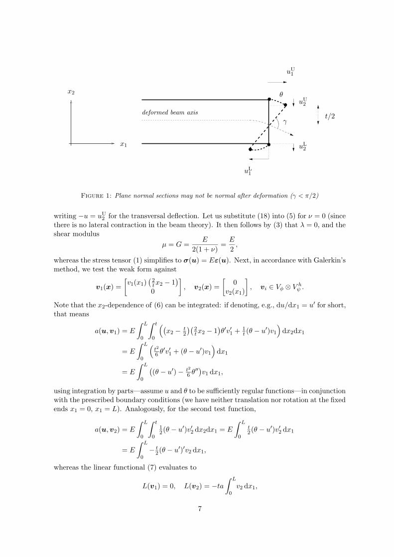
PSfrag replacements

uL1

uU1

θ

x1

x2

uL2

uU2

deformed beam axis

γt/2

Figure 1: Plane normal sections may not be normal after deformation (γ < π/2)

writing −u = uU2 for the transversal deflection. Let us substitute (18) into (5) for ν = 0 (since

there is no lateral contraction in the beam theory). It then follows by (3) that λ = 0, and theshear modulus

µ = G =E

2(1 + ν)=E

2,

whereas the stress tensor (1) simplifies to σ(u) = Eε(u). Next, in accordance with Galerkin’smethod, we test the weak form against

v1(x) =[v1(x1)

(2tx2 − 1

)0

], v2(x) =

[0

v2(x1)

], vi ∈ Vφ ⊗ V h

ψ .

Note that the x2-dependence of (6) can be integrated: if denoting, e.g., du/dx1 = u′ for short,that means

a(u,v1) = E

∫ L

0

∫ t

0

((x2 − t

2

)(2tx2 − 1

)θ′v′1 + 1

t (θ − u′)v1)

dx2dx1

= E

∫ L

0

(t2

6 θ′v′1 + (θ − u′)v1

)dx1

= E

∫ L

0

((θ − u′)− t2

6 θ′′)v1 dx1,

using integration by parts—assume u and θ to be sufficiently regular functions—in conjunctionwith the prescribed boundary conditions (we have neither translation nor rotation at the fixedends x1 = 0, x1 = L). Analogously, for the second test function,

a(u,v2) = E

∫ L

0

∫ t

0

12(θ − u′)v′2 dx2dx1 = E

∫ L

0

t2(θ − u′)v′2 dx1

= E

∫ L

0− t

2(θ − u′)′v2 dx1,

whereas the linear functional (7) evaluates to

L(v1) = 0, L(v2) = −ta∫ L

0v2 dx1,

7

since the inner products f · v1 = 0, f · v2 = −av2. Now, by standard arguments (see, e.g., [5,Chapter 8.1.2]), we may expect the weighted averages∫ L

0

[E

((θ − u′)− t2

6 θ′′)]v1 dx1 = 0,∫ L

0

[− Et2 (θ − u′)′ + ta

]v2 dx1 = 0,

to actually hold pointwise, and thereby we identify the strong forms

Et

2d

dx1

(dudx1

− θ

)= −ta, (19)

Et2

6d2θ

dx21

+ E

(dudx1

− θ

)= 0. (20)

If substituting (20) into (19) we obtain the system of ODEsEt3

12d3θ

dx31

= ta

dudx1

= θ − t2

6d2θ

dx21

(21)

which relates closely to (15). To see this, set I = t3/12, f = ta in the first equation, and thenfor the second, observe that

EI

AκG=

t2

6κ,

by using E/G = 2, A = wt = t.In conclusion, making appropriate assumptions on the kinematic and constitutive relations

in (5), allows for reducing the weak formulation to 1D, by integrating along the thickness of thebeam. We retrieve the equations of the Timoshenko beam theory, apart from an absent shearcoefficient κ, which compensates for the shear stress not being uniform over the cross-sectionR (it has a parabolic shape). Experimental data for a rectangular R suggests how

κ =5(1 + ν)6 + 5ν

=56, if ν = 0,

according to [8]. Note that (21) approaches (14) as t→ 0, i.e., this model corresponds exactlyto the Bernoulli beam theory in the limiting case (just as (15) does).

Remark. We emphasize that the additional kinematic relations (17) imposed on the solution,actually means that it does not belong to our model hierarchy, and consequently, neither doesthe Timoshenko beam. However, (21) then suggests the thin domain approach, in our setting,to be a natural extension of the beam theories, with less constraints on the solution.

4 A Posteriori Error Estimate

We pose two auxiliary problems: Find uψ ∈ V hφ ⊗ Vψ and uφ ∈ Vφ ⊗ V h

ψ such that

a(uψ,v) = L(v), ∀v ∈ V hφ ⊗ Vψ, (22)

a(uφ,v) = L(v), ∀v ∈ Vφ ⊗ V hψ , (23)

8

where the tensor-product solutions are semi-discrete (exact in one variable and approximatein the other). We shall outline estimates of the total error in energy norm

‖e‖a = ‖u− uh‖a := a(u− uh,u− uh)1/2,

which uncouple terms representing the effects of the discretization and model errors. For thispurpose, we consider (22) and (23) separately, first observing that

‖u− uh‖a = ‖u− uψ + uψ − uh‖a ≤ ‖u− uψ‖a + ‖uψ − uh‖a (24)

by the triangle inequality. The terms of the right-hand side are bounded, which we motivateby studying eψ = uψ − uh. Let πh : V h

φ ⊗ Vψ → V hφ ⊗ V h

ψ be a standard nodal interpolationoperator1 (or the L2-projection), and note that

‖uψ − uh‖2a = a(uψ − uh, eψ)

(25)= a(uψ − uh, eψ − πhu

ψ)(11)= L(eψ − πhu

ψ)− a(uh, eψ − πhuψ),

using the energy orthogonality

a(uψ − uh,v) = 0, ∀v ∈ V hφ ⊗ V h

ψ . (25)

Elementwise integration by parts of the second term gives

‖uψ − uh‖2a =

∑K∈Th

∫K

(f + div(σ(uh)) · (eψ − πheψ) dx

+∫∂ΩN

g · (eψ − πheψ) ds

−∑K∈Th

∫∂K

σ(uh) · nK · (eψ − πheψ) ds,

for nK being the outward unit normal of the element boundary. Since each E ∈ EhI is commonto two elements, we may regroup terms as

‖uψ − uh‖2a =

∑K∈Th

∫K

(f + div(σ(uh)) · (eψ − πheψ) dx

+∫∂ΩN

(g − σ(uh) · n) · (eψ − πheψ) ds

+∑E∈EhI

∫E[σ(uh) · nE ] · (eψ − πhe

ψ) ds,

where we define

[σ(uh) · nE ](x) := limε→0+

((σ · nE)(x + εnE)− (σ · nE)(x− εnE)

), x ∈ E,

1The existence of such an interpolant is guaranteed, since v ∈ Vφ ⊗ Vψ ⊂ H2 by assumption, and thus haspointwise values (see [9, Chapter 5.3]).

9

to be the jump in traction across the element edge E with unit normal nE . Then, by meansof Cauchy’s inequality and suitable estimates of the interpolation error eψ − πhe

ψ, followingJohnson and Hansbo [7, Theorem 2.1], we eventually arrive at

‖uψ − uh‖a ≤ C1

(‖hR1(uh)‖L2(Ω) + ‖hR2(uh)‖L2(Ω)

), (26)

where

R1(uh) = |R1(uh)|, R2(uh) = h1/2 ‖R2(uh)‖L2(∂Ω)

V (K),

with V (K) as the volume of K, and

R1(uh) = f + div(σ(uh)), on K, K ∈ Th,

R2(uh) =

12 [σ(uh) · nE ]/hK , on E, E ∈ EhI ,(g − σ(uh) · n)/hK , on E, E ∈ EhB.

R1 and R2 represent the residuals related to the interior and the boundary of each element,respectively, whereas C1 is a bounded interpolation constant, typically computable by a finitedimensional eigenvalue problem, see, e.g., [7, Equation 2.9, Section 2.3]. In the same manner,with πh : Vφ ⊗ Vψ → V h

φ ⊗ Vψ, using the orthogonality relation

a(u− uψ,v) = 0, ∀v ∈ V hφ ⊗ Vψ,

we obtain‖u− uψ‖a ≤ C2

(‖hR1(uψ)‖L2(Ω) + ‖hR2(uψ)‖L2(Ω)

), (27)

Then, by adding and subtracting uφ in (24), analogous arguments eventually lead to

‖uφ − uh‖a ≤ C3

(‖hR1(uh)‖L2(Ω) + ‖hR2(uh)‖L2(Ω)

), (28)

‖u− uφ‖a ≤ C4

(‖hR1(uφ)‖L2(Ω) + ‖hR2(uφ)‖L2(Ω)

). (29)

We assume the residuals (27) and (29), from the semi-discrete spaces, to be smaller than theirdiscrete counterparts (26) and (28), i.e.,

‖u− uψ‖a = (1− α)‖uψ − uh‖a, ‖u− uφ‖a = (1− β)‖uφ − uh‖a,

for some 0 ≤ α, β ≤ 1. This, given α = β = 0, implies

‖u− uh‖a ≤ 2‖uψ − uh‖a, ‖u− uh‖a ≤ 2‖uφ − uh‖a,

as upper bounds of the total error, in terms of the model and discretization errors, respectively.It follows directly

‖u− uh‖a ≤ ‖uψ − uh‖a + ‖uφ − uh‖a, (30)

or, with C = C1 + C3,

‖u− uh‖a ≤ C(‖hR1(uh)‖L2(Ω) + ‖hR2(uh)‖L2(Ω)

), (31)

which is an (completely discretized) a posteriori error estimate.

10

Remark. The computational mesh is subjected to geometrical anisotropy—the elements havedifferent dimension in different directions (one element spans the thickness of the domain, soh(x) → t, as more elements are introduced; see Section 5.2 for details). The a posteriori errorestimate (31) does not take this into account, but doing so may lead to sharper error bounds.An example indicating how to get improved estimates is discussed in [7, Section 2.4]. We didnot pursue this here.

5 Implementation

5.1 Fundamental concepts

Using adaptivity requires some tools, e.g., a suitable norm in which the error e = u − uh ismeasured. In Section 4 the focus was on the energy norm ‖·‖a = a(·, ·)1/2, seeing uh as theminimizer to ‖u− v‖a over V h

ψ ⊗ V hψ . Note how (8) states that uh, as compared to u, has a

larger potential energy. Hence, since F (u) may be expressed in terms of the energy norm,

F (u) = 12a(u,u)− L(u) = 1

2a(u,u)− a(u,u) = − 12‖u‖2

a,

the relation ‖uh‖a ≤ ‖u‖a holds, so the computed strains ε(uh) are underestimated, and thenumerical problem gets too stiff. In Section 4 we used the well-known energy orthogonality

a(e,v) = 0, ∀v ∈ V hψ ⊗ V h

ψ , (32)

stating how the error e is orthogonal to the subspace V hψ ⊗V h

ψ . Important relations involvingthe energy norm can be derived from (32), e.g., the best approximation property

‖u− uh‖a = infv‖u− v‖a, v ∈ V h

ψ ⊗ V hψ ,

which implies any refined FE-solution ui to have larger energy norm, i.e.,

‖ui‖a ≥ ‖ui−1‖a, i = 1, 2, . . . , (33)

since we are solving a minimization problem with respect to a larger function space. Anotherrelation is the equality

‖e‖2a = a(u− uh,u− uh) = a(u,u− uh)− a(uh,u− uh)

(32)= a(u,u− uh)

= a(u,u)− a(u,uh)(32)= a(u,u)− a(u,uh)− a(uh − u,uh)

= a(u,u)− a(uh,uh) = ‖u‖2a − ‖uh‖2

a,

(34)

which holds only in energy norm.

5.2 The element

In Section 2 we mentioned the nodal basis, and to elaborate, tensor-product Lagrangian finiteelements were implemented. The basis functions are constructed by means of one-dimensionalLagrange polynomials

ln−1i =

(x− x1) · · · (x− xi−1)(x− xi+1) · · · (x− xn)(xi − x1) · · · (xi − xi−1)(xi − xi+1) · · · (xi − xn)

, i = 1, 2, . . . , n, (35)

11

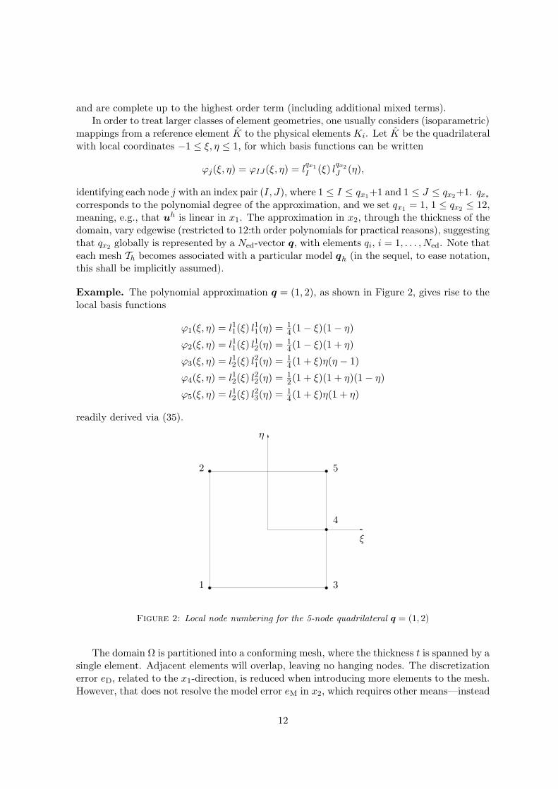
and are complete up to the highest order term (including additional mixed terms).In order to treat larger classes of element geometries, one usually considers (isoparametric)

mappings from a reference element K to the physical elements Ki. Let K be the quadrilateralwith local coordinates −1 ≤ ξ, η ≤ 1, for which basis functions can be written

ϕj(ξ, η) = ϕIJ(ξ, η) = lqx1I (ξ) lqx2J (η),

identifying each node j with an index pair (I, J), where 1 ≤ I ≤ qx1+1 and 1 ≤ J ≤ qx2+1. qx∗corresponds to the polynomial degree of the approximation, and we set qx1 = 1, 1 ≤ qx2 ≤ 12,meaning, e.g., that uh is linear in x1. The approximation in x2, through the thickness of thedomain, vary edgewise (restricted to 12:th order polynomials for practical reasons), suggestingthat qx2 globally is represented by a Ned-vector q, with elements qi, i = 1, . . . , Ned. Note thateach mesh Th becomes associated with a particular model qh (in the sequel, to ease notation,this shall be implicitly assumed).

Example. The polynomial approximation q = (1, 2), as shown in Figure 2, gives rise to thelocal basis functions

ϕ1(ξ, η) = l11(ξ) l11(η) = 1

4(1− ξ)(1− η)

ϕ2(ξ, η) = l11(ξ) l12(η) = 1

4(1− ξ)(1 + η)

ϕ3(ξ, η) = l12(ξ) l21(η) = 1

4(1 + ξ)η(η − 1)

ϕ4(ξ, η) = l12(ξ) l22(η) = 1

2(1 + ξ)(1 + η)(1− η)

ϕ5(ξ, η) = l12(ξ) l23(η) = 1

4(1 + ξ)η(1 + η)

readily derived via (35).

PSfrag replacements

ξ

η

1

2

3

4

5

Figure 2: Local node numbering for the 5-node quadrilateral q = (1, 2)

The domain Ω is partitioned into a conforming mesh, where the thickness t is spanned by asingle element. Adjacent elements will overlap, leaving no hanging nodes. The discretizationerror eD, related to the x1-direction, is reduced when introducing more elements to the mesh.However, that does not resolve the model error eM in x2, which requires other means—instead

12

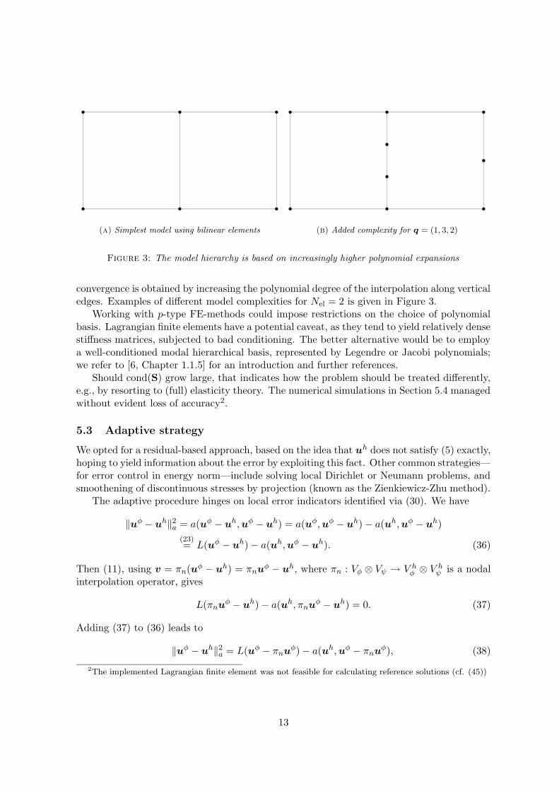
(a) Simplest model using bilinear elements (b) Added complexity for q = (1, 3, 2)

Figure 3: The model hierarchy is based on increasingly higher polynomial expansions

convergence is obtained by increasing the polynomial degree of the interpolation along verticaledges. Examples of different model complexities for Nel = 2 is given in Figure 3.

Working with p-type FE-methods could impose restrictions on the choice of polynomialbasis. Lagrangian finite elements have a potential caveat, as they tend to yield relatively densestiffness matrices, subjected to bad conditioning. The better alternative would be to employa well-conditioned modal hierarchical basis, represented by Legendre or Jacobi polynomials;we refer to [6, Chapter 1.1.5] for an introduction and further references.

Should cond(S) grow large, that indicates how the problem should be treated differently,e.g., by resorting to (full) elasticity theory. The numerical simulations in Section 5.4 managedwithout evident loss of accuracy2.

5.3 Adaptive strategy

We opted for a residual-based approach, based on the idea that uh does not satisfy (5) exactly,hoping to yield information about the error by exploiting this fact. Other common strategies—for error control in energy norm—include solving local Dirichlet or Neumann problems, andsmoothening of discontinuous stresses by projection (known as the Zienkiewicz-Zhu method).

The adaptive procedure hinges on local error indicators identified via (30). We have

‖uφ − uh‖2a = a(uφ − uh,uφ − uh) = a(uφ,uφ − uh)− a(uh,uφ − uh)

(23)= L(uφ − uh)− a(uh,uφ − uh). (36)

Then (11), using v = πn(uφ − uh) = πnuφ − uh, where πn : Vφ ⊗ Vψ → V h

φ ⊗ V hψ is a nodal

interpolation operator, gives

L(πnuφ − uh)− a(uh, πnuφ − uh) = 0. (37)

Adding (37) to (36) leads to

‖uφ − uh‖2a = L(uφ − πnu

φ)− a(uh,uφ − πnuφ), (38)

2The implemented Lagrangian finite element was not feasible for calculating reference solutions (cf. (45))

13

and analogously

‖uψ − uh‖2a = L(uψ − πnu

ψ)− a(uh,uψ − πnuψ), (39)

representing the effects of the discretization and model errors. (The rationale behind (38) and(39), in the present context, are on the subtle side, since (36) gives equal estimates. Includingthe interpolant provides standard error estimates for further analysis.)

The functions uφ and uψ have to be discretized, and therefore we pose the problems: Finduφ ∈ V ∗

φ ⊗ V hψ and uψ ∈ V h

φ ⊗ V ∗ψ such that

a(uφ,v) = L(v), ∀v ∈ V ∗φ ⊗ V h

ψ , (40)

a(uψ,v) = L(v), ∀v ∈ V hφ ⊗ V ∗

ψ , (41)

seeking enhanced FE-solutions as approximations. The function spaces V ∗φ ⊗V h

ψ and V hφ ⊗V ∗

ψ

are defined with respect to Th: (40) is solved on a bisected mesh Tφ, having twice the numberof elements as Th, with added vertical edges inheriting maxqi, qi+1 from the parent elementKi, exemplified by q = (1, 3, 2) → (1, 3, 3, 3, 2) (the children retain the highest order term ofthe parental approximation). (41) is solved on a mesh Tψ, with the same number of elementsas Th, but qi → qi + 1 (all polynomial degrees along vertical edges are raised by 1), so thatq = (1, 3, 2) → (2, 4, 3). Since

‖uφ − uh‖2a =

Nel∑i=1

‖uφ − uh‖2a,Ki ,

(38) and (39) suggest the computable local error indicators

eD,K = L(uφ − πnuφ)K − a(uh, uφ − πnu

φ)K , (42)

eM,K = L(uψ − πnuψ)K − a(uh, uψ − πnu

ψ)K , (43)

where assessing (43) typically requires less degrees of freedom, but also yields a denser stiffnessmatrix S, due to more connections between neighbors (cf. computational cost below). In eachiteration a fixed ratio r of the local error indicators—the largest absolute values regardless oferror source—have their corresponding elements marked for refinement (neighbors subjectedto model refinement have qi raised by 1 on common edges). Notice that this direct comparisonof local indicators is justified by (30).

The approach is straightforward, benefits from controlling the sizes3 of the refined meshand model, but becomes insensitive to presence of local singularities (then tends to overrefine).Any initial mesh/model T0 should not be too coarse (typically we want the error to fall withinthe asymptotic convergence rate of the error produced by pure h-refinement).

The reliability of the local error indicators is validated by the effectivity index

θ =(∑eD,K)1/2 + (

∑eM, K)1/2

‖u− uh‖a =eest‖e‖a , (44)

which ideally remains constant during the adaptive refinement, thus indicating the algorithmto converge with the same order as the underlying FE-method. If unknown, the exact solution

3The more sophisticated strategy would be to predict the actual mesh size and model required to achievethe prescribed accuracy.

14

u was approximated by a reference solution u, which substitutes into the denominator of (44)as e = ‖u− uh‖a. For that purpose we state the problem: Find u ∈ V h × V h such that

a(u,v) = L(v), ∀v ∈ V h × V h, (45)

where V h is the space of piecewise continuous quadratic functions (which vanishes on ∂ΩD).The reference solution was resolved on a dense uniform triangulation Tr (Nd(Tr) = 5 254 146).

Remark. We emphasize that (30) foremost is a motivation behind (42) and (43), i.e., selectingelements for refinement, rather than providing accurate error control. When approximatingthe semi-discrete solutions by (40) and (41), it follows from (33) and (34) that

‖uφ − uh‖a − ‖uφ − uh‖a = ‖uφ‖2a − ‖uφ‖2

a ≥ 0 =⇒ ‖uφ‖a ≥ ‖uφ‖a,which means we may lose the upper bound quality of (30). (This property is ensured by (31)for an upper bound of the interpolation constant, but we get no information on how to updatemesh and model. Also, since (31) employs Cauchy’s inequality on each element, it could yieldconsiderable overestimations.)

A crude—but implementation independent—estimate of the computational cost for solvingthe primal problem is

Nd(Th) = 2Ned∑i=1

qi + 2Ned,

in terms of the number of degrees of freedom Nd (mesh dependent). The adaptive procedureinvolves solving two refined problems in each iteration, to the separate costs

Nd(Tφ) = Nd(Th) + 2Nel∑i=1

maxqi, qi+1+ 2Nel,

Nd(Tψ) = Nd(Th) + 2Ned,

where Ned = Ned(Th), Nel = Nel(Th). If assuming |qi − qi+1| ≤ 1 we get

2Nel∑i=1

maxqi, qi+1 ≤Nel∑i=1

(qi + qi+1 + 1) < 2Ned∑i=1

qi +Nel = Nd(Th) +Nel − 2Ned,

and thus the total cost becomes

Nd(Tφ) +Nd(Tψ) < 3(Nd(Th) +Nel

), (46)

about three times the primal cost of solving (11). Moreover, (46) does not include calculatingthe local error indicators, and hence the overall procedure is more expensive, even though thecost of solving (40) and (41) is larger.

As for stopping criterion, the adaptive algorithm, detailed in Algorithm 1, halted once thefinest model was locally introduced, i.e., if any qi = qmax = 11 (the last polynomial degree isreserved for uψ). This was done for purpose of evaluation—a user-specified tolerance TOL isused in practice.

The implementation utilized a direct sparse Cholesky solver [3, 4] for solving the matrixproblem (12).

15

Algorithm 1: Adaptive scheme

Data: initial mesh T0

Result: FE-solution uh, internal energy ‖uh‖2a, estimated total error eest

Let ∗ denote either sub- and superscripts φ and ψ

for j = 0, 1, . . . do

solve primal problem (11) for uh on Tjcalculate internal energy ‖uh‖2

a

solve refined problems (40) and (41) for u∗ on T∗for i = 1, . . . , Nel do

calculate local error indicators eD,Ki and eM,Ki via (42) and (43)end

estimate total error eestmark elements for refinement (h, q or hq)if any qi = qmax then

breakelse

refine mesh and model: Tj → Tj+1

end

end

5.4 Numerical results

Cantilever beam. Let Ω be the unit square 0 ≤ x1, x2 ≤ 1, which is kept fixed at x1 = 0,and subjected to a surface traction g = (0,−1) at x2 = 1. The material parameters are E = 1and ν = 0.3. The domain is not typically thin, but the solution, according to [1, p. 2170], hasthe exact internal energy ‖u‖2

a = 1.903697, and makes a suitable reference.

The problem was solved adaptively for an initial configuration Nel = 10, qi = 3 and r = 0.15.Consecutive updates of mesh and model, Tj → Tj+1, j = 0, 1, 2, . . ., were dominated by themodel error. The finest local model was introduced after 9 iterations, when the overall modelcomplexity corresponded to 58 % of the finest global model:

%(model) = 100 · Nd −min(Nd)max(Nd)−min(Nd)

,

where Nd = Nd(Tj). Extreme values relate to the present refinement level j, such that

min(Nd) = Nd(Tj ; qi = 1), max(Nd) = Nd(Tj ; qi = qmax).

The refinements were concentrated at the clamped end x1 = 0, coinciding with large stressesand strains, close to the points x1 = (0, 1), x2 = (0, 0). The accuracy of ‖uh9‖a came within0.2 %, not possible for the bilinear approximation (the simplest model at hand), for which‖uh‖2

a / 1.559. Figure 4 further advocates the benefits of model adaptivity: the successive FE-solutions were more accurate than those obtained by uniform triangular P 2-approximations(according to (45) for subsequent mesh sizes h =

√5/4, 1/2,

√5/8, 1/4,

√5/16). We normally

expect singularities to be difficult to resolve using higher-order polynomial interpolations (the

16

exact solution would not be differentiable). Therefore the small error is somewhat surprising—uh still manages to capture the local behavior of u in the vicinity of x1 and x2. In [1] therefinement strategy was another (based on the Zienkiewicz-Zhu method, trying to predict themesh size), employing a bilinear approximation (not in a thin domain setting); the energywas ‖uh‖2

a = 1.89289 over 718 degrees of freedom. This is less accurate than our FE-solution,which, however, was superseded at 964 degrees of freedom. Figure 6(a) shows the local error

100 1000

0.1

0.2

PSfrag replacements

Nd

‖e‖ a

t = 1

hqP 2

Figure 4: Comparing model adaptivity (hq) and uniform triangular P 2-approximations

contributions (40) and (41) to be of similar order, apart from a larger model error at x1 = 0.The effectivity index θ, defined in (44), remained fairly constant, and judging by the dataenclosed in Table 1, it also provides accurate error control. The triangle inequality leading to(24) approximately overestimated the total error by a factor C ≈ 1.3-1.4

‖u− uh‖a = C(‖u− uφ‖a + ‖uφ − uh‖a

),

‖u− uh‖a = C(‖u− uψ‖a + ‖uψ − uh‖a

),

during the iterative procedure; alongside the FE-solutions uφ and uφ having smaller energynorms (as compared to their semi-discrete counterparts), that may, at least in some extent,account for θ ≈ 1.

Reducing the domain thickness (t → 1/10) induced a shift towards h-refinement, suggestinghow higher polynomial expansions are less important, when nature of the problem turns one-dimensional. The accuracy of ‖uh14‖a—with respect to a reference solution ‖u‖2

a = 1.903687(the surface traction was scaled, g = (0,−0.058582), to preserve the internal energy)—wasless than 0.02 %, implying a linear improvement with respect to t. In Table 2 the data showsthat 26.8 % of the finest model was used at the last refinement level, the first instance of q-refinement occurring at the 7:th iteration. Figure 6(b) indicates large variations in the modelerror at x1 = 0, which suggests how the singularities cause problems after all (at least by being

17

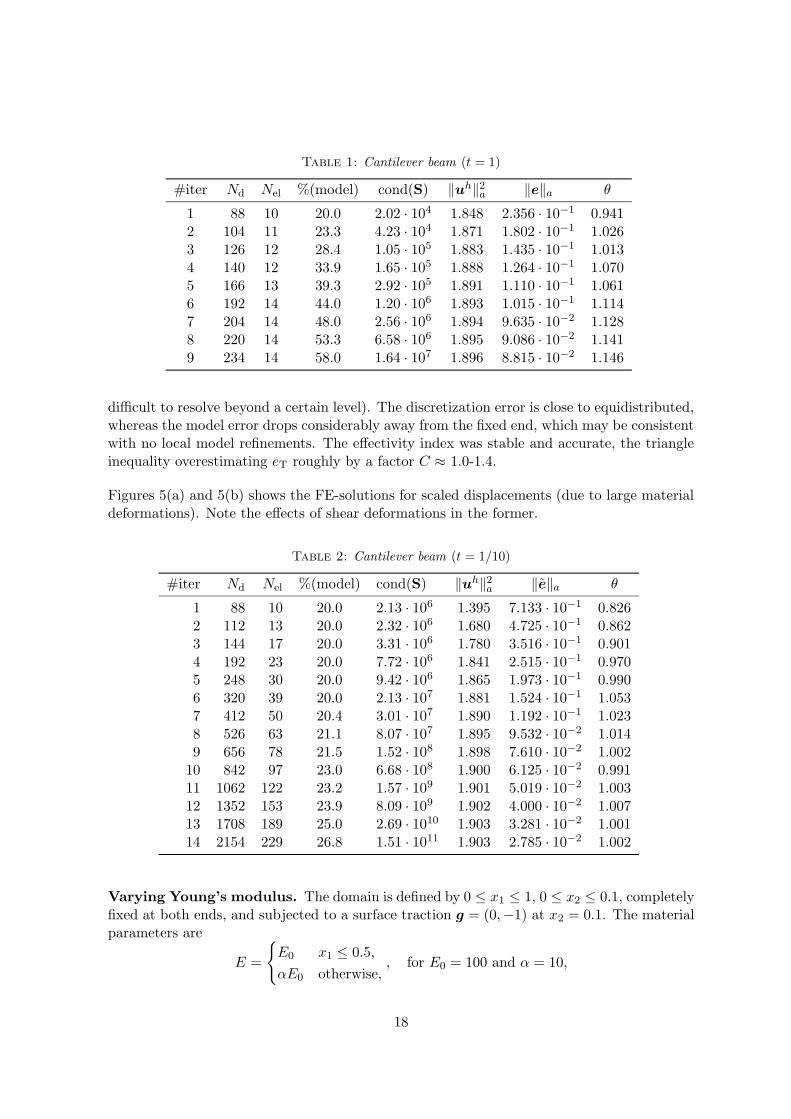
Table 1: Cantilever beam (t = 1)

#iter Nd Nel %(model) cond(S) ‖uh‖2a ‖e‖a θ

1 88 10 20.0 2.02 · 104 1.848 2.356 · 10−1 0.9412 104 11 23.3 4.23 · 104 1.871 1.802 · 10−1 1.0263 126 12 28.4 1.05 · 105 1.883 1.435 · 10−1 1.0134 140 12 33.9 1.65 · 105 1.888 1.264 · 10−1 1.0705 166 13 39.3 2.92 · 105 1.891 1.110 · 10−1 1.0616 192 14 44.0 1.20 · 106 1.893 1.015 · 10−1 1.1147 204 14 48.0 2.56 · 106 1.894 9.635 · 10−2 1.1288 220 14 53.3 6.58 · 106 1.895 9.086 · 10−2 1.1419 234 14 58.0 1.64 · 107 1.896 8.815 · 10−2 1.146

difficult to resolve beyond a certain level). The discretization error is close to equidistributed,whereas the model error drops considerably away from the fixed end, which may be consistentwith no local model refinements. The effectivity index was stable and accurate, the triangleinequality overestimating eT roughly by a factor C ≈ 1.0-1.4.

Figures 5(a) and 5(b) shows the FE-solutions for scaled displacements (due to large materialdeformations). Note the effects of shear deformations in the former.

Table 2: Cantilever beam (t = 1/10)


1 88 10 20.0 2.13 · 106 1.395 7.133 · 10−1 0.8262 112 13 20.0 2.32 · 106 1.680 4.725 · 10−1 0.8623 144 17 20.0 3.31 · 106 1.780 3.516 · 10−1 0.9014 192 23 20.0 7.72 · 106 1.841 2.515 · 10−1 0.9705 248 30 20.0 9.42 · 106 1.865 1.973 · 10−1 0.9906 320 39 20.0 2.13 · 107 1.881 1.524 · 10−1 1.0537 412 50 20.4 3.01 · 107 1.890 1.192 · 10−1 1.0238 526 63 21.1 8.07 · 107 1.895 9.532 · 10−2 1.0149 656 78 21.5 1.52 · 108 1.898 7.610 · 10−2 1.002

10 842 97 23.0 6.68 · 108 1.900 6.125 · 10−2 0.99111 1062 122 23.2 1.57 · 109 1.901 5.019 · 10−2 1.00312 1352 153 23.9 8.09 · 109 1.902 4.000 · 10−2 1.00713 1708 189 25.0 2.69 · 1010 1.903 3.281 · 10−2 1.00114 2154 229 26.8 1.51 · 1011 1.903 2.785 · 10−2 1.002

Varying Young’s modulus. The domain is defined by 0 ≤ x1 ≤ 1, 0 ≤ x2 ≤ 0.1, completelyfixed at both ends, and subjected to a surface traction g = (0,−1) at x2 = 0.1. The materialparameters are

E =

E0 x1 ≤ 0.5,αE0 otherwise,

, for E0 = 100 and α = 10,

18

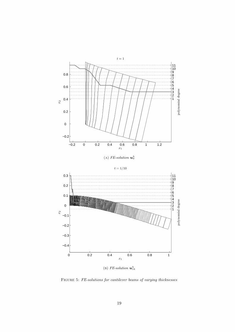
−0.2 0 0.2 0.4 0.6 0.8 1 1.2

−0.2

0

0.2

0.4

0.6

0.8

1 2 3 4 5 6 7 8 9 1011

PSfrag replacements

x1

x2

poly

nom

ialdeg

ree

t = 1

(a) FE-solution uh9

0 0.2 0.4 0.6 0.8 1

−0.4

−0.3

−0.2

−0.1

0

0.1

0.2

0.3

1 2 3 4 5 6 7 8 9 1011

PSfrag replacements

x1

x2

poly

nom

ialdeg

ree

t = 1/10

(b) FE-solution uh14

Figure 5: FE-solutions for cantilever beams of varying thicknesses

19

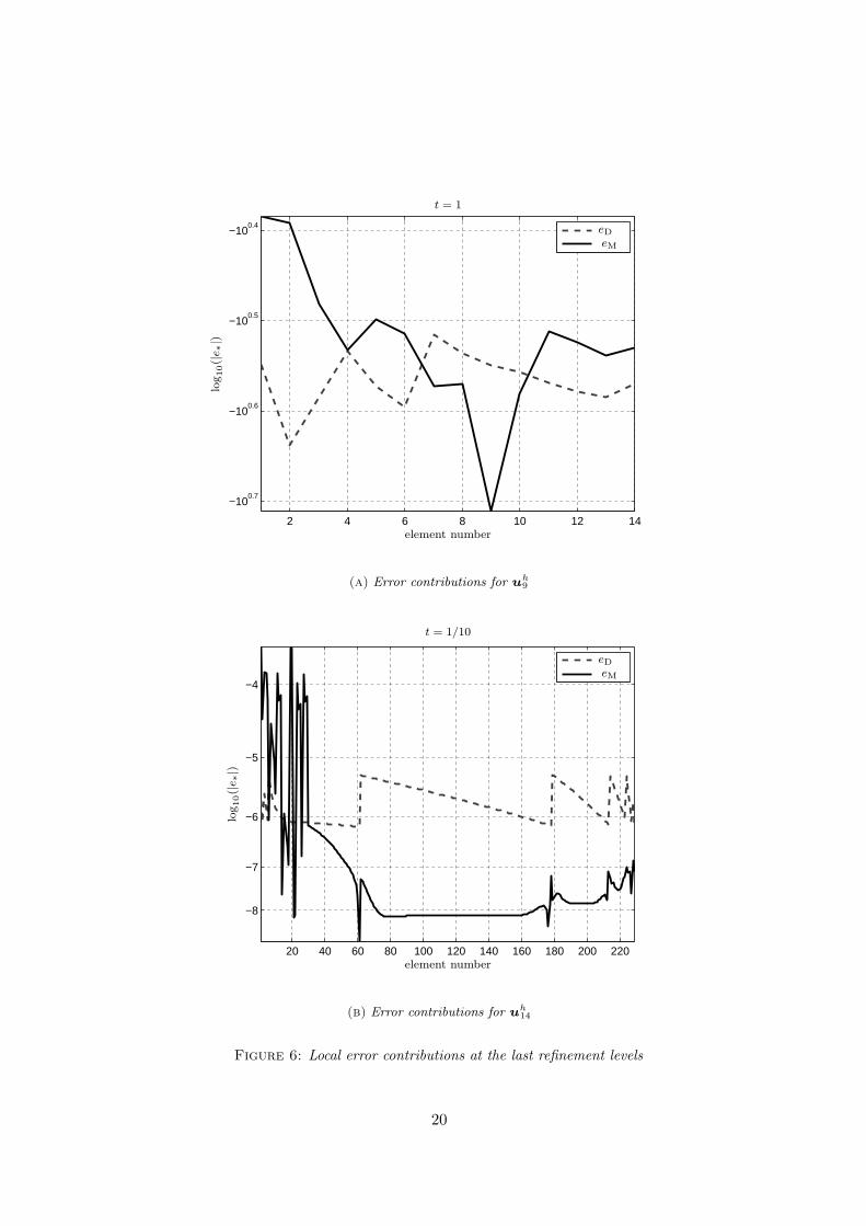
2 4 6 8 10 12 14

−100.4

−100.5

−100.6

−100.7

PSfrag replacements

element number

log10(|e

∗|)eDeM

t = 1

(a) Error contributions for uh9

20 40 60 80 100 120 140 160 180 200 220

−4

−5

−6

−7

−8

PSfrag replacements

element number

log10(|e

∗|)

eDeM

t = 1/10

(b) Error contributions for uh14

Figure 6: Local error contributions at the last refinement levels

20

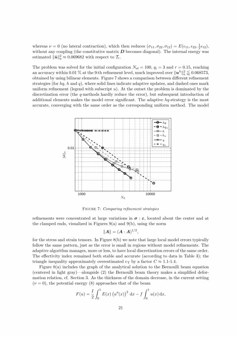
whereas ν = 0 (no lateral contraction), which then reduces (σ11, σ22, σ12) = E(ε11, ε22, 12ε12),

without any coupling (the constitutive matrix D becomes diagonal). The internal energy wasestimated ‖u‖2

a ≈ 0.069682 with respect to Tr.

The problem was solved for the initial configuration Nel = 100, qi = 3 and r = 0.15, reachingan accuracy within 0.01 % at the 9:th refinement level, much improved over ‖uh‖2

a / 0.068573,obtained by using bilinear elements. Figure 7 shows a comparison between different refinementstrategies (for hq, h and q), where solid lines indicate adaptive updates, and dashed ones markuniform refinement (legend with subscript u). At the outset the problem is dominated by thediscretization error (the q-methods hardly reduce the error), but subsequent introduction ofadditional elements makes the model error significant. The adaptive hq-strategy is the mostaccurate, converging with the same order as the corresponding uniform method. The model

1000 10000

0.01

PSfrag replacements

Nd

‖e‖ a

hq

hquh

hu

q

qu

Figure 7: Comparing refinement strategies

refinements were concentrated at large variations in σ : ε, located about the center and atthe clamped ends, visualized in Figures 9(a) and 9(b), using the norm

‖A‖ = (A : A)1/2,

for the stress and strain tensors. In Figure 8(b) we note that large local model errors typicallyfollow the same pattern, just as the error is small in regions without model refinements. Theadaptive algorithm manages, more or less, to have local discretization errors of the same order.The effectivity index remained both stable and accurate (according to data in Table 3); thetriangle inequality approximately overestimated eT by a factor C ≈ 1.1-1.4.

Figure 8(a) includes the graph of the analytical solution to the Bernoulli beam equation(centered in light gray)—alongside (2) the Bernoulli beam theory makes a simplified defor-mation relation, cf. Section 3. As the thickness of the domain decrease, in the current setting(ν = 0), the potential energy (8) approaches that of the beam

F (u) =I

2

∫ 1

0E(x)

(u′′(x)

)2 dx− f

∫ 1

0u(x) dx,

21

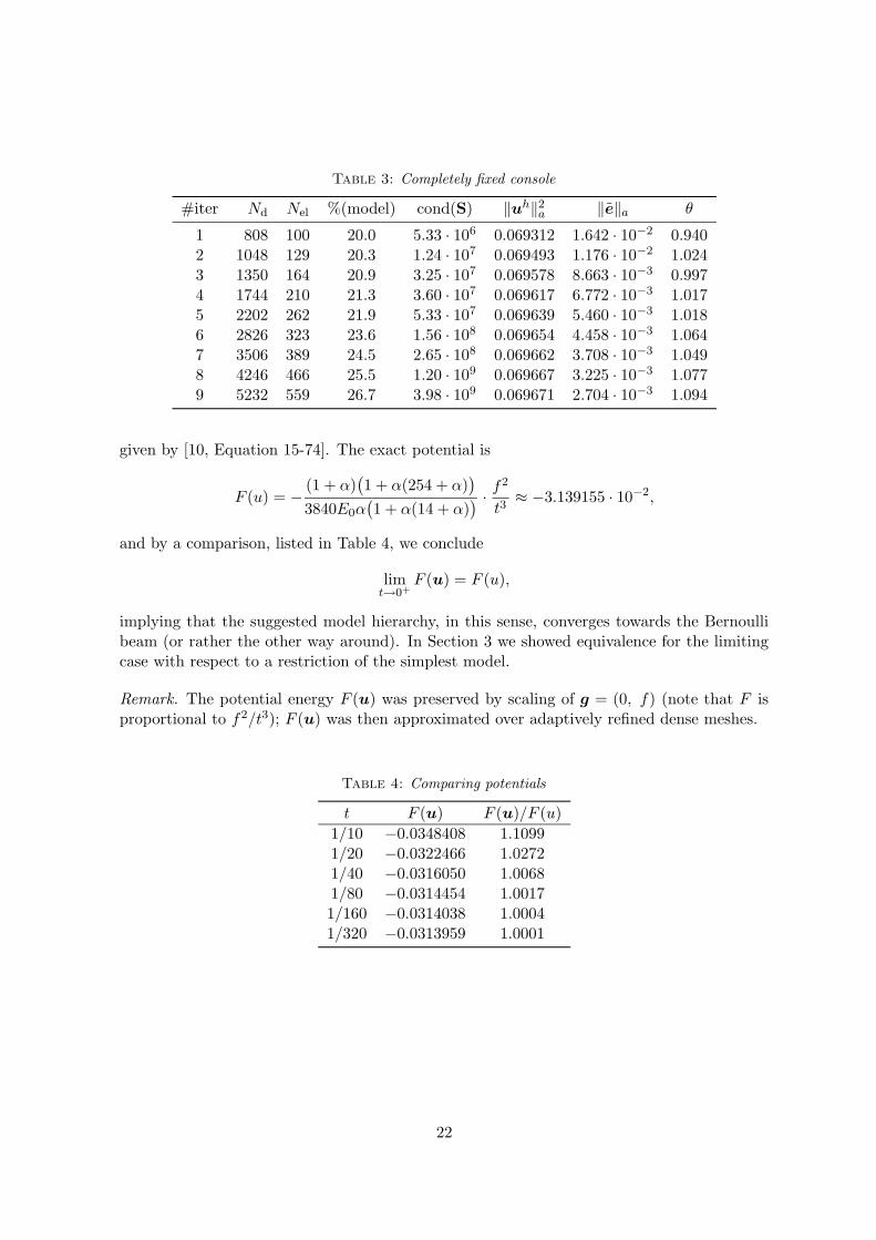
Table 3: Completely fixed console


1 808 100 20.0 5.33 · 106 0.069312 1.642 · 10−2 0.9402 1048 129 20.3 1.24 · 107 0.069493 1.176 · 10−2 1.0243 1350 164 20.9 3.25 · 107 0.069578 8.663 · 10−3 0.9974 1744 210 21.3 3.60 · 107 0.069617 6.772 · 10−3 1.0175 2202 262 21.9 5.33 · 107 0.069639 5.460 · 10−3 1.0186 2826 323 23.6 1.56 · 108 0.069654 4.458 · 10−3 1.0647 3506 389 24.5 2.65 · 108 0.069662 3.708 · 10−3 1.0498 4246 466 25.5 1.20 · 109 0.069667 3.225 · 10−3 1.0779 5232 559 26.7 3.98 · 109 0.069671 2.704 · 10−3 1.094

given by [10, Equation 15-74]. The exact potential is

F (u) = − (1 + α)(1 + α(254 + α)

)3840E0α

(1 + α(14 + α)

) · f2

t3≈ −3.139155 · 10−2,

and by a comparison, listed in Table 4, we conclude

limt→0+

F (u) = F (u),

implying that the suggested model hierarchy, in this sense, converges towards the Bernoullibeam (or rather the other way around). In Section 3 we showed equivalence for the limitingcase with respect to a restriction of the simplest model.

Remark. The potential energy F (u) was preserved by scaling of g = (0, f) (note that F isproportional to f2/t3); F (u) was then approximated over adaptively refined dense meshes.

Table 4: Comparing potentials

t F (u) F (u)/F (u)1/10 −0.0348408 1.10991/20 −0.0322466 1.02721/40 −0.0316050 1.00681/80 −0.0314454 1.00171/160 −0.0314038 1.00041/320 −0.0313959 1.0001

22

6 Conclusions

We summarize the results of the paper in the following list:

The semi-discrete energy error estimate (30) provides a basis for an adaptive procedure,which, in the light of the examples in Section 5.4, seems not only reliable, but capableof sharp error control (which we have to admit is not obvious).

The local error indicators (40) and (41) concentrated the updates of mesh and model tolarge variations in stresses and strains, i.e., at locations where we expect a predominanterror.

The accuracy of the FE-solutions were generally high, even when the physical domainhad L/t = 1 (unit square), but we stress that this is not the typical thin domain setting.Refining the model adaptively was necessary to maintain efficiency; otherwise simplermodels degenerate as eD → 0.

The suggested model hierarchy would be a natural extension to a larger hierarchy, bybridging the Bernoulli and Timoshenko beam theories with the (full) elasticity theory.

23

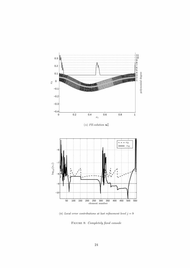
0 0.2 0.4 0.6 0.8 1 −0.4

−0.3

−0.2

−0.1

0

0.1

0.2

0.3

1 2 3 4 5 6 7 8 9 1011

PSfrag replacements

x1

x2

poly

nom

ialdeg

ree

(a) FE-solution uh9

50 100 150 200 250 300 350 400 450 500 550

−9

−10

−6

−7

−8

PSfrag replacements

element number

log10(|e

∗|)

eDeM

(b) Local error contributions at last refinement level j = 9

Figure 8: Completely fixed console

24

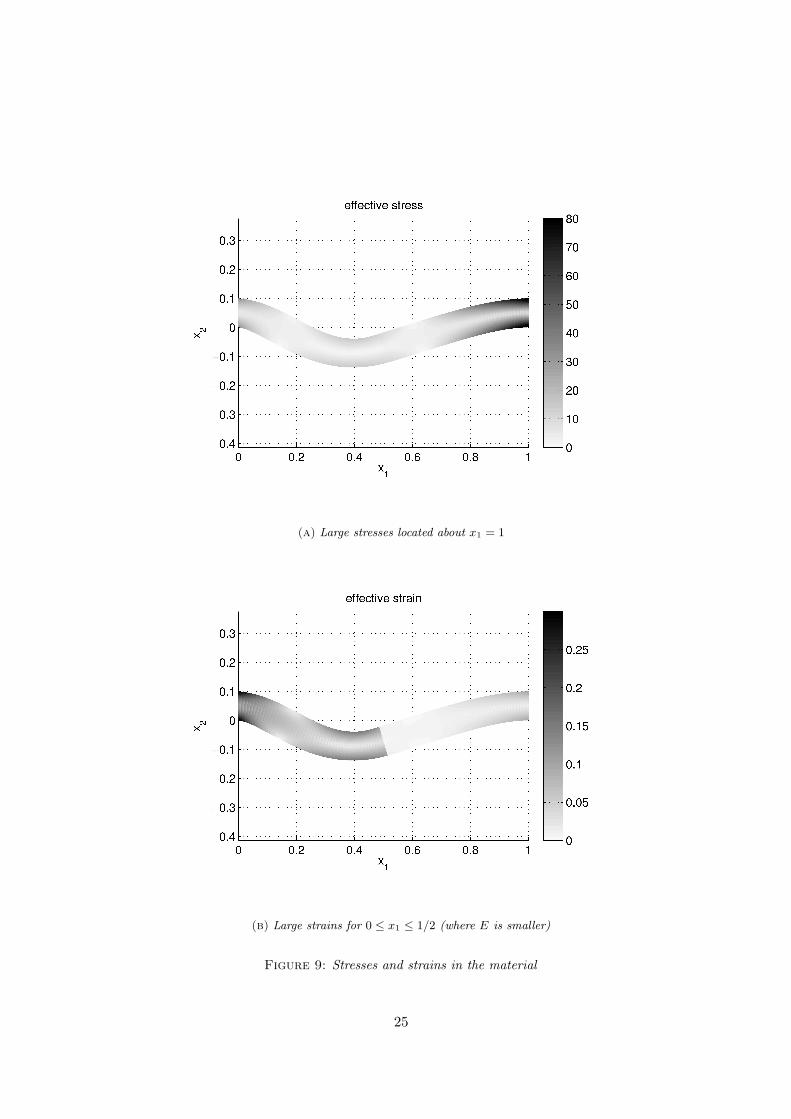
PSfrag replacements

x1

x2

Effective stress

(a) Large stresses located about x1 = 1

PSfrag replacements

x1

x2

Effective strain

(b) Large strains for 0 ≤ x1 ≤ 1/2 (where E is smaller)

Figure 9: Stresses and strains in the material

25

References

[1] M. Ainsworth, J. Z. Zhu, A. W. Craig, and O. C. Zienkiewicz, Analysis of the Zienkiewicz-Zhu a posteriori error estimator in the finite element method, International Journal forNumerical Methods in Engineering 28 (1989), 2161–2174.

[2] I. Babuska, I. Lee, and C. Schwab, On the a posteriori estimation on the modeling errorfor the heat conduction in a plate and its use for adaptive hierarchial modeling, AppliedNumerical Mathematics 14 (1994), 5–21.

[3] Yanqing Chen, Timothy A. Davis, William W. Hager, and Sivasankaran Rajaman-ickam, Algorithm 887: CHOLMOD, Supernodal Sparse Cholesky Factorization and Up-date/Downdate, ACM Transactions on Mathematical Software 35 (2008), no. 3.

[4] Timothy A. Davis and William W. Hager, Dynamic Supernodes in Sparse Cholesky Up-date/Downdate and Triangular Solvers, ACM Transactions on Mathematical Software35 (2008), no. 4.

[5] K. Eriksson, D. Estep, P. Hansbo, and C. Johnson, Computational differential equations,Studentlitteratur, 1996.

[6] A. Ern and J-L. Guermond, Theory and practice of finite elements, Springer-Verlag,2004.

[7] C. Johnson and P. Hansbo, Adaptive finite element methods in computational mechanics,Computer Methods in Applied Mechanics and Engineering 101 (1992), 143–181.

[8] T. Kaneko, On Timoshenko’s correction for shear in vibrating beams, Journal of PhysicsD: Applied Physics 8 (1975), 1927–1936.

[9] S. Larsson and V. Thomee, Partial Differential Equations with Numerical Methods,Springer-Verlag, 2003.

[10] H. Lundh, Grundlaggande hallfasthetslara, 3:rd ed., Kungliga tekniska hogskolan, 2000.

[11] N. S. Ottosen and H. Petersson, Introduction to the finite element method, Prentice HallEurope, 1992.

[12] W. Weaver (JR), S. P. Timoshenko, and D.H. Young, Vibration problems in engineering,5:th ed., John Wiley and Sons, 1990.

26

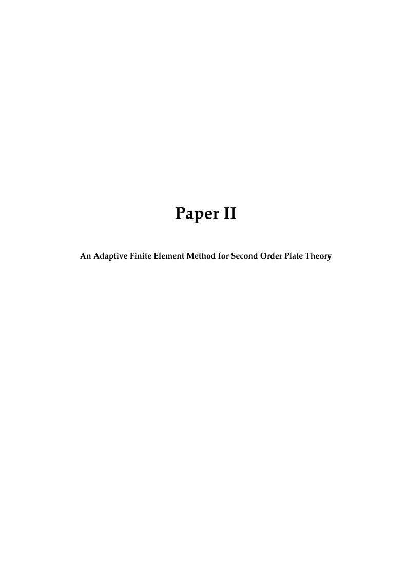
Paper II

An Adaptive Finite Element Method for Second Order Plate Theory

An adaptive finite element method for second order

plate theory

Peter Hansbo1, David Heintz1 and Mats G. Larson2

1 Department of Mathematics, Chalmers University of Technology and University ofGothenburg, SE–412 96 Goteborg, Sweden

2 Department of Mathematics and Mathematical Statistics, Umea University, SE–90187 Umea, Sweden

Abstract

We present a discontinuous finite element method for the Kirchhoff plate model withmembrane stresses. The method is based on P 2−approximations on simplices for theout-of-plane deformations, using C0−continuous approximations. We derive a posteriorierror estimates for linear functionals of the error and give some numerical examples.

1 INTRODUCTION

Kirchhoff plate deformation analysis is often carried out without taking into account the effectof in-plane stresses. However, if these are significant or if a stability analysis is required, thefourth order plate equations must be supplemented with a second order term. In such acase, standard finite element methods for plates may not be well suited for the problem;an example of this is the well known Morley plate element which is known not to convergefor the Laplace equation, cf. [7]. In this paper we instead use the continuous/discontinuousGalerkin method first proposed by Engel et al. [2], and proposed (using a different but relatedformulation) for second order theory by Wells and Dung [8]. In this paper, we focus on usingcontinuous piecewise second degree polynomials (with discontinuous derivatives) for the plateand constant–strain elements for the in-plane deformations. We present an a posteriori erroranalysis including the modeling error in the stresses. The total error is thus composed oftwo parts: the plate discretization error and the error emanating from the modeling of thestresses. In our case the stress error is also a discretization error, which allows for a posterioricontrol of the total error. However, the separation of the errors allows for the use, e.g., ofmeasured stresses, in which case some other control of the error in stresses must be used if areliable estimate is to be obtained.

1

2 THE PLATE MODEL

Consider a domain Ω ⊂ R2, for simplicity assumed to be a convex polygon, whose boundary∂Ω has an outward pointing normal n. The plate thickness in the out-of-plane x3−direction isdenoted by t, and the deflection in the x3−direction by u. The differential equations describingthe Kirchhoff plate model with membrane stresses can be derived from minimization of thesum of the bending energy and the potential of the surface and in-plane stress load,

Uz(u) =D

2

∫Ω

((∂2u

∂x21

+∂2u

∂x22

)2

− 2 (1 − ν)

(∂2u

∂x21

∂2u

∂x22

−

(∂2u

∂x1∂x2

)2))

dΩ

+t

2

∫Ω

(σ11

(∂u

∂x1

)2

+ σ22

(∂u

∂x2

)2

+ 2σ12∂u

∂x1

∂u

∂x2

)dΩ −

∫Ω

g u dΩ

(1)

where g is the transverse surface load,

σ =

[σ11 σ12

σ12 σ22

]is the in-plane stress tensor, given by the solution to the plane stress problem

−∇ · σ = f in Ω,

σ = σ(u) := 2µε(u) + λ∇ · u1,

where λ = Eν/(1 − ν2) and µ = E/(2 (1 + ν)); D = Et3/(12(1 − ν2)) is the flexural rigidityof the plate, and E and ν are Young’s modulus and Poisson’s ratio, respectively.

In the following, we shall assume that if the stresses are compressive, they are small enoughto ensure coercivity of the full problem; the case of large compressive stresses occurs in theanalysis of plate buckling, where the potential energy functional switches from being convexto being concave, resulting in instability.

By introducing the curvature tensor

κ(u) :=

∂2u

∂x21

∂2u

∂x1∂x2

∂2u

∂x1∂x2

∂2u

∂x22

the Lame–type parameters µP := D(1 − ν)/2, and λP := Dν, and the moment tensor

M(u) := 2µPκ(u) + λP∆u1

where 1 is the identity tensor, we may rewrite (1) as

U(u) =1

2

∫Ω

(M(u) : κ(u) + t (σ∇u) · ∇u − 2gu) dΩ (2)

where M : κ =∑

ij Mijκij denotes the contraction of two tensors. Minimization of (2) yieldsthe plate equation with second order effects∑

ij

(∂2Mij(u)

∂xi∂xj−

∂

∂xi

(tσij

∂u

∂xj

))= g in Ω, (3)

2

supplied with the appropriate boundary conditions.For simplicity, we shall restrict the presentation to the case of clamped boundary condi-

tions: n · ∇u = 0 and u = 0 on ∂Ω. We shall also assume that the constitutive parametersand the thickness are constant.

3 THE FINITE ELEMENT METHOD

3.1 Variational formulation

The virtual work equation related to (3) is the following variational statement: find

u ∈ V := v : v ∈ H2(Ω), v = 0 on ∂Ω, n · ∇v = 0 on ∂Ω

such thataP(u, v) + b(σ; u, v) = (g, v)

for all v ∈ V , where

aP(u, v) :=

∫Ω

M(u) : κ(v) dΩ,

b(σ; u, v) := t

∫Ω(σ∇u) · ∇v dΩ.

To obtain σ, we also have to solve the plane stress problem of finding u ∈ W := [H10 (Ω)]2

such that(σ(u), ε(v)) = (f , v) ∀v ∈ W , (4)

where

(σ(u), ε(v)) :=

∫Ω

σ(u) : ε(v) dΩ

In the following, we shall also use the L2 scalar product notation

(u, v)E :=

∫E

u v ds, (M , τ )T :=

∫T

M : τ dxdy, etc.

If the subscript is omitted, the product is taken over Ω.

3.2 Finite element method

We consider a subdivision T = T of Ω into a geometrically conforming, quasiuniform, sim-plicial finite element mesh. Denote by hT the diameter of element T and by h = maxT∈T hT

the global mesh size parameter. We shall use continuous, piecewise polynomial, approxima-tions of the transverse displacement:

Vh := v ∈ H10 (Ω) ∩ C0(Ω) : v|T ∈ P 2(T ), ∀T ∈ T .

To define our methods we introduce the set of edges in the mesh, E = E, and we splitE into two disjoint subsets

E = EI ∪ EB,

where EI is the set of edges in the interior of Ω and EB is the set of edges on the boundary.Further, with each edge we associate a fixed unit normal n such that for edges on the boundary

3

n is the exterior unit normal. We denote the jump of a function v ∈ Γh at an edge E by[v] = v+ − v− for E ∈ EI and [v] = v+ for E ∈ EB, and the average 〈v〉 = (v+ + v−)/2 forE ∈ EI and 〈v〉 = v+ for E ∈ EB, where v± = limε↓0 v(x ∓ ε n) with x ∈ E.

Our method can now be formulated as follows: find uh ∈ Vh such that

ahP(uh, v) + b(σ; uh, v) = (g, v) (5)

for all v ∈ Vh. In (5) the bilinear form ahP(·, ·) is defined on Vh as follows

ahP(u, v) =

∑T∈T

(M(u), κ(v))T

−∑

E∈EI∪EB

(〈n · M(u) · n〉, [n · ∇v])E

−∑

E∈EI∪EB

(〈n · M(v) · n〉, [n · ∇u])E

+ (2µ + 2λ) γ0

∑E∈EI∪EB

h−1E ([n · ∇u], [n · ∇v])E

Here γ0 is a constant whose role is to enforce coercivity of the form ahP(·, ·), and hE is defined

byhE =

(|T+| + |T−|

)/(2 |E|) for E = ∂T+ ∩ ∂T−, (6)

with |T | the area of T , on each edge. Precise values for the choice of γ0 are given in [5].Using Green’s formula, we readily establish the following Lemma.

Lemma 1 The method (5) is consistent in the sense that

ahP(u − uh, v) + b(σ; u − uh, v) = 0 (7)

for all v ∈ Vh.

Now, the σ in (5) is the exact stress solution to the problem (4) which we cannot solve exactlyin general. Instead we introduce the discrete problem of finding uh ∈ W h, where

W h := v ∈ W ∩ [C0(Ω)]2 : v|T ∈ [P 1(T )]2, ∀T ∈ T ,

such that(σ(uh), ε(v)) = (f , v) ∀v ∈ W h. (8)

Using the notation σh := σ(uh), our discrete plate problem becomes: find uh ∈ Vh such that

ahP(uh, v) + b(σh; uh, v) = (g, v) (9)

for all v ∈ Vh, and the orthogonality relation (7) is weakened to

ahP(u − uh, v) + b(σ; u, v) − b(σh; uh, v) = 0, ∀v ∈ Vh. (10)

4

3.3 An approach to a posteriori error estimation

Since the error in the discrete plate problem (9) does not couple to the plane stress problem(8), we shall here follow Larson and Bengzon [3] and view the fact that we must replace σ byσh as a modeling error.

Following Becker and Rannacher [1], we are interested in controlling a linear functionalL(u − uh) of the error (where L is to be specified), and to this end we introduce the dualproblem of finding z such that∑

ij

(∂2Mij(z)

∂xi∂xj−

∂

∂xi

(tσh

ij

∂z

∂xj

))= J in Ω, (11)

z = 0 and n · ∇z = 0 on ∂Ω. Here J is the Riesz representer of L, L(v) = (J, v). Then, since[n · ∇z] = 0 on the edges,

(J, e) = L(u − uh) = ahP(z, u − uh) + b(σh; z, u − uh)

= ahP(u − uh, z) + b(σh; u − uh, z) + b(σ; u, z) − b(σ; u, z)

= (g, z − πhz) − ahP(uh, z − πhz) − b(σh; uh, z − πhz)

+ b(σh − σ; u, z),

(12)

where we used (10) in the last step.Since σ − σh = σ(u − uh), we can now introduce a second functional, related to the

modelling error.Lmod(u − uh) := −b(σ(u − uh); u, z)

and the dual problem of finding z ∈ W such that

(σ(v), ε(z)) = Lmod(v) ∀v ∈ W .

Thus, the functional Lmod of the error can be evaluated as

Lmod(u − uh) = (σ(u − uh), ε(z))

= (f , z − πhz) − (σh, ε(z − πhz)),

where we used that(σ(u) − σ(uh), ε(v)) = 0, ∀v ∈ W h.

In conclusion, we have that

L(u − uh) = (g, z − πhz) − ahP(uh, z − πhz) − b(σh; uh, z − πhz)

+ (f , z − πhz) − (σh, ε(z − πhz)).(13)

In (13), the error contribution has thus been split between discretization errors for theplate (the terms involving z−πhz) and the model error (in this case discretization error) in thestresses (the terms involving z − πhz). The continuous stresses do not enter directly into thediscretization error for the plate; the effect of using approximate stresses has been separatedout. In case the stresses have been obtained in some other way, e.g., by measurement, (12)can instead be used together with some direct estimate of the stress error.

5

4 IMPLEMENTATION

We seek to establish a practical adaptive scheme, such that a linear functional L(·) of theerror, e = u − uh, is bounded. To that end, duality-based techniques are employed, whichinclude solving enriched problems—the corresponding dual problems—to distribute degreesof freedom in an efficient manner. In our numerical examples, the datum of the dual plateproblem (11), i.e., the target quantity, is chosen as a Dirac delta function

J := δ(x1 − x1, x2 − x2), (14)

where (x1, x2) is the node of maximum plate deflection (whose location is expected to convergerather quickly as the mesh size h → 0). As opposed to estimating the error with respect toglobal energy norms or global L2-norms, (14) exemplifies a typical local quantity, which oftenis more appropriate in applications.

The linear functional (13) was written as a sum, L(e) = ηP + ηM, where

ηP = (g, z − πhz) − ahP(uh, z − πhz) − b(σh; uh, z − πhz), (15)

ηM = (f , z − πhz) − (σh, ε(z − πhz)), (16)

represent the effects of the discretization and model errors. This provides alternatives for thediscretization of the domain Ω:

(i) use a common partition T (quadratic and linear triangles for the plate and plane stressproblems coincide geometrically);

(ii) use disparate triangulations TP and TM.

The first option associates each element Ti ∈ T with an error indicator

ηi = |ηiP| + |ηi

M|, i = 1, 2, . . . , N, (17)

where N is the number of elements of T . This choice makes for an easier implementation, butthe information from (15) and (16) is not thoroughly exploited, since we resort to sums of localerrors contributions. The more flexible approach—in keeping with model adaptivity—wouldbe a direct comparison, made possible by disparate triangulations. However, this necessitatesmaking searches when solving the point-in-triangle problem (see, e.g., [9, Algorithm 4]),usually preceded by constructing a suitable search structure, a so-called binary tree or quadtree; we refer to [10] for further details. In the present context, the need for such searchestypically arise when basis functions are evaluated in abscissas (query points), situated ondifferent elements (targets) between TP and TM.

Remark 1 Preprocessing Ω into a search structure comes at a cost, and although intendedto ease the effort, it still takes time to perform searches (the procedure ought to be parallelizedsince individual queries are independent). The winnings are increased flexibility in distributingthe degrees of freedom, thereby yielding smaller matrix problems achieving the same level ofaccuracy.

In the sequel the discussion focuses on using disparate meshes (the other case being areduced analog), where TP and TM are assumed to consist of NP and NM elements, respectively.Hence, instead of (17), consider the concatenated (NP + NM)-tuple

η =(η1P, . . . , ηNP

P , η1M, . . . , ηNM

M

), (18)

6

from which we select a fixed ratio r of the largest absolute local error indicators, regardlessof the error source, and mark the corresponding elements for refinement. The primal meshesare updated via a Bansch-algorithm (longest edge bisection) leaving no hanging nodes.

In order to determine (18) we need to approximate exact solutions. Therefore we introducetwo auxiliary problems: Find u ∈ V ∗

h and z ∈ V ∗h such that

ahP(u, v) + b(σh; u, v) = (g, v), ∀v ∈ V ∗

h ,

ahP(v, z) + b(σh; v, z) = L(v), ∀v ∈ V ∗

h ,

which assemble the same stiffness matrix, only deviating by the RHS-data (thus passed to-gether as arguments to a direct sparse Cholesky solver). The solutions are then used as inputto the discretized dual plane stress problem: Find z ∈ W ∗

h such that

(σ(v), ε(z)) = −b(σ(v); u, z), ∀v ∈ W ∗h.

The enriched function spaces V ∗h ⊃ Vh and W ∗

h ⊃ W h are constructed by subjecting theprimal partitions to regular subdivision, leading to the refined triangulations TP and TM,respectively. When calculating local error indicators by (15) and (16), πhv : V ∗

h → Vh andπhv : W ∗

h → W h were taken, for simplicity, to be nodal interpolation operators.The stopping criterion of the adaptive algorithm is imposed on the relative error

erel :=

∣∣∣∣ L(e)

u(x1, x2)

∣∣∣∣ ≤ TOL,

where

L(e) = LP + LM, LP =

NP∑j=1

ηjP, LM =

NM∑k=1

ηkM,

and TOL is a prescribed tolerance. Furthermore, let

|LP| =

NP∑j=1

|ηjP|, |LM| =

NM∑k=1

|ηkM|,

denote the sums of the absolute local error indicators. The adaptive scheme is summarizedin Algorithm 1.

Remark 2 The bilinear form ahP contains a penalty term, controlling the normal derivative,

which is scaled by a parameter γ0. From [5] a lower bound of γ0 > 3CI, where CI is a constantthat depends on the order k of the approximation, ensures its coercivity. For this purpose weset γ0 = 3/2 in all test problems, using the asymptotic value of the constant.

The a posteriori error estimator is evaluated in terms of the effectivity index

θ :=

∣∣∣∣L(e)

L(e)

∣∣∣∣ =

∣∣∣∣ L(e)

u(x1, x2) − uh(x1, x2)

∣∣∣∣ ,

where u(x1, x2) is a reference solution replacing the unknown exact maximum plate deflection.u was obtained by solving the primal problems adaptively on a common dense mesh T .

The adaptive procedure is rather time-consuming—in every iteration two dual problemsare solved (including the enhanced discrete plate problem). An effort to reduce the compu-tational cost would be to solve the problems with respect to their primal FE-spaces, followedby post-processing to obtain solutions in enriched function spaces, see, e.g., Larsson et al. [6].

7

Algorithm 1: Adaptive scheme

Data: initial mesh T 0, user-specified tolerance TOLResult: FE-solution uh, total error L(e)

for i = 0, 1, . . . do

solve primal plane stress problem for σh on T iM

solve primal plate problem for uh on T iP

construct dual meshes T iP and T i

M

solve primal and dual plate problems for u and z on T iP

solve dual plane stress problem for z on T iM

compute local error indicators ηjP and ηk

M

if TOL > erel then

refine primal meshes: T iP → T i+1

P , T iM → T i+1

M

elsebreak

end

end

5 NUMERICAL EXAMPLES

Algorithm 1 is applied to a set of test problems, which is not meant to be comprehensive,but to exemplify the behavior of the a posteriori error estimator. We shall compare twoadaptive strategies: 1) refine a common mesh T i (referred to as the CM-method); and 2)refine disparate meshes T i

P and T iM (DM-method). Note that

the transversal and in-plane boundary conditions are different in each setup;

the load—either f or g—causing the stress field σ is restricted to maintain the positive-definiteness of the stiffness matrix (typically the loading must not be too large);

the refinement ratio is set to r = 0.2.

Remark 3 The computational cost—per degree of freedom—associated with the plate problemis larger (than for the plane stress problem), partly due to the symmetry and penalty termsof the ah

P-functional, alongside the additional b-functional. Consequently, having a relativelysmall plate problem could be beneficial, and hence relevant results are presented with respectto: 1) the total number of degrees of freedom DT = DP + DM; and 2) the number of degreesof freedom for the plate problem DP.

5.1 Point Load on Unit Square

Consider the plate Ω = [0, 1] × [0, 1], simply supported (so that u = 0 at ∂Ω) and fixed onthe left side (u|x1=0 = 0). The material parameters are ν = 0.3, E = 100, and the thicknesst = 0.1. The plate carries a point load at xl = (1/4, 3/4), whereas in-plane stresses areinduced by a surface traction g = (0, −1) at x2 = 1.

8

The plane stress FE-formulation now becomes: Find uh ∈ W h such that

(σ(uh), v) = (g, v)∂ΩN, ∀v ∈ W h,

where ∂ΩN denotes the Neumann boundary x2 = 1, and the local model error indicator (16)changes accordingly

ηM = (g, z − πhz)∂ΩN− (σh, ε(z − πhz)).

The point load is applied to a single node, and thus the discrete load vector fP = δij , so that(15) reduces to

ηP = −ahP(uh, z − πhz) − b(σh; uh, z − πhz).

The FE-solutions of the plate and plane stress problems are shown in Figures 1 and 2 (the lat-ter uses non-deformed coordinates): the maximum plate deflection (cross-marked) is situatedclose to xi (circle-marked), whereas large effective stresses

σe := (σ : σ)1/2

appear in the vicinity of the vertices (0, 0), (0, 1).Consecutive updates of T were presumably dominated by the discretization error, as

implied by Table 1, where the larger and strictly decreasing LP (almost) sums up to the totalerror L(e) (disregarding cancellation effects). Refinements are concentrated around xl, asseen in Figure 6, and hence one anticipates NP > NM, should disparate meshes be used. Thisis also the case, being confirmed by Table 2 and Figure 14(a), showing the shift towards TP-refinement as most prominent during the initial iterations. When comparing the two meshesin Figures 7 and 8, note the difference at the large-stress vertices, where consequently TM isrefined while TP is not, following the almost symmetric (along the line x2 = 1−x1) refinementpattern of T instead (further underlining the importance of the discretization error).

The adaptive algorithm is superior to uniform refinement, according to Figures 15(a) and15(b), where the latter indicates how the DM-method avoids unnecessary model complexity,i.e., results in a coarser mesh TM, and still satisfies the prescribed relative error TOL = 5·10−3.

The effectivity indices are stable—we obtain convergence rates of the same order as theunderlying FE-method—and the accuracy is high (θ → 1+ in Figure 13(a)).

5.2 An L-shaped Membrane

Let Ω be the polygon with vertices (0, 0), (c, 0), (c, c), (1, c), (1, 1) and (0, 1) for c = 1/2, havingmaterial parameters ν = 0.3, E = 100, and the thickness t = 0.1. The plate is subjectedto a uniform load g = 1, and carries an in-plane point load at the tip xl = (1, 1), such thatf(xl) = (0,−4). It is simply supported (u = 0 at ∂Ω) and fixed on the left side (u|x1=0 = 0).

In this setting, with the point load applied in a single node, the discretized load vectorfM = δij , and (16) reduces to

ηM = −(σh, ε(z − πhz)),

otherwise (15) and the FE-formulations remain unchanged.

The maximum plate deflection (cross-marked in Figure 6) would occur along the symmetryline x2 = 1 − x1 (dashed), had it not been for large planar stresses at xl, and particularlyaround the non-convex corner singularity; thereby max uh deviates to (x1, x2) ≈ (0.26, 0.51).

9

The influence of the large stresses implies how the model error now becomes more promi-nent. Tables 3 and 4 concurs that LP and LM are of the same order of magnitude (note thatthe cancellation effects are greater for the model error)—the DM-method recognizes this andconcentrates refinements on TM (emphasized by Figure 14(b)). During the adaptive procedureadditional elements are foremostly introduced at the interior corner (1/2, 1/2), but TP is alsoresolved around (x1, x2).

Using an adaptive algorithm is favorable, judging by Figure 16, and the solution improvesas the complexity of the model increases. The tolerance was TOL = 2 · 10−2.

The total error is slightly underestimated, but the effectivity indices remain fairly stable,and grow slowly (Figure 13(b) shows that θ → 1−).

6 CONCLUDING REMARKS

We have presented a C0 finite element element method for second-order analysis of thinplates. A posteriori error estimates for linear functionals of the error have been derived. Ournumerical examples, focusing on controlling the error in maximum deflection, show that theestimates give effectivity indices close to unity.

References

[1] Becker R, Rannacher R. A feed-back approach to error control in finite element methods:basic analysis and examples. East-West Journal of Numerical Mathematics 1996; 4:237–264.

[2] Engel G, Garikipati K, Hughes TJR, Larson MG, Mazzei L, Taylor RL. Continu-ous/discontinuous finite element approximations of fourth-order elliptic problems instructural and continuum mechanics with applications to thin beams and plates, andstrain gradient elasticity. Computer Methods in Applied Mechanics and Engineering 2002;191:3669–3750.

[3] Larson MG, Bengzon F. Adaptive finite element approximation of multiphysics problems.Communications in Numerical Methods in Engineering 2008; 24:505–521.

[4] Hansbo P, M.G. Larson MG. A discontinuous Galerkin method for the plate problem.Calcolo 2002; 39:41–59.

[5] Hansbo P, Larson MG. A posteriori error estimates for continuous/discontinuousGalerkin approximations of the Kirchhoff-Love plate. Preprint (2008).

[6] Larsson F, Hansbo P, Runesson K. Strategies for computing goal-oriented a posteriorierror measures in non-linear elasticity. International Journal for Numerical Methods inEngineering 2002; 55:879–894.

[7] Nilssen TK, Tai XC, Winther R. A robust nonconforming H2-element. Mathematics ofComputation 2001; 70:489–505.

[8] Wells GN, Dung, NT. A C0 discontinuous Galerkin formulation for Kirchhoff plates.Computer Methods in Applied Mechanics and Engineering 2007; 196:3370–3380.

10

[9] Svensson ED. Optimal search in finite element triangulations using binary trees. Preprint(Department of Mathematical Sciences, Division of Mathematics, Chalmers Universityof Technology and Goteborg University), 2006:21, 1652-9715.

[10] O’Rourke J. Computational geometry in C. 2:nd ed., Cambridge University Press, 1998.

11

Table 1: Common mesh T# DP DM LP LM L(e) θ

1 545 290 2.81 · 10−2 1.26 · 10−4 3.15 · 10−2 0.902 668 356 2.57 · 10−2 9.90 · 10−5 2.16 · 10−2 1.203 839 442 1.22 · 10−2 6.33 · 10−5 1.32 · 10−2 0.934 1071 562 9.72 · 10−3 1.53 · 10−5 9.53 · 10−3 1.025 1412 736 7.70 · 10−3 1.59 · 10−5 7.34 · 10−3 1.056 1861 962 5.64 · 10−3 1.54 · 10−5 5.45 · 10−3 1.047 2453 1262 4.35 · 10−3 1.74 · 10−5 4.23 · 10−3 1.038 3230 1660 3.37 · 10−3 1.24 · 10−5 3.28 · 10−3 1.039 4328 2214 2.63 · 10−3 3.57 · 10−6 2.52 · 10−3 1.04

10 5780 2946 1.97 · 10−3 2.34 · 10−6 1.91 · 10−3 1.0311 7659 3890 1.46 · 10−3 4.80 · 10−6 1.43 · 10−3 1.0212 10185 5168 1.11 · 10−3 3.16 · 10−6 1.10 · 10−3 1.01

Table 2: Disparate meshes TP and TM

# DP DM LP LM L(e) θ

1 545 290 2.81 · 10−2 1.27 · 10−4 3.15 · 10−2 0.902 739 308 2.35 · 10−2 9.37 · 10−5 1.98 · 10−2 1.193 1001 336 9.06 · 10−3 7.26 · 10−5 1.05 · 10−2 0.874 1409 382 7.36 · 10−3 1.95 · 10−5 7.21 · 10−3 1.025 1933 438 5.24 · 10−3 1.41 · 10−5 5.16 · 10−3 1.026 2662 526 4.07 · 10−3 1.81 · 10−5 3.94 · 10−3 1.047 3615 650 2.90 · 10−3 1.01 · 10−5 2.84 · 10−3 1.038 4909 848 2.32 · 10−3 5.47 · 10−6 2.25 · 10−3 1.039 6558 1128 1.71 · 10−3 9.98 · 10−6 1.69 · 10−3 1.02

10 8638 1508 1.32 · 10−3 7.14 · 10−6 1.31 · 10−3 1.0111 11483 1990 1.02 · 10−3 4.19 · 10−6 1.01 · 10−3 1.01

Iterations during adaptive procedure (unit square)

12

Table 3: Common mesh T# DP DM LP LM |LP| |LM| L(e) θ

1 833 450 9.53 · 10−3 2.31 · 10−3 1.16 · 10−2 1.26 · 10−2 1.46 · 10−2 0.812 1029 548 7.25 · 10−3 2.32 · 10−3 8.66 · 10−3 1.11 · 10−2 1.17 · 10−2 0.823 1304 688 5.53 · 10−3 1.96 · 10−3 7.59 · 10−3 1.00 · 10−2 8.83 · 10−3 0.854 1662 868 4.29 · 10−3 1.53 · 10−3 6.18 · 10−3 8.46 · 10−3 6.81 · 10−3 0.855 2147 1114 3.30 · 10−3 1.13 · 10−3 5.07 · 10−3 7.71 · 10−3 5.05 · 10−3 0.886 2798 1446 2.57 · 10−3 1.01 · 10−3 4.06 · 10−3 6.92 · 10−3 4.11 · 10−3 0.877 3635 1870 2.06 · 10−3 7.67 · 10−4 3.62 · 10−3 6.20 · 10−3 3.17 · 10−3 0.898 4774 2442 1.58 · 10−3 6.14 · 10−4 3.17 · 10−3 5.44 · 10−3 2.50 · 10−3 0.889 6268 3196 1.25 · 10−3 4.42 · 10−4 2.62 · 10−3 4.60 · 10−3 1.87 · 10−3 0.91

10 8164 4152 9.68 · 10−4 3.32 · 10−4 2.25 · 10−3 4.08 · 10−3 1.42 · 10−3 0.9111 10600 5384 7.76 · 10−4 2.61 · 10−4 1.84 · 10−3 3.61 · 10−3 1.11 · 10−3 0.93

Table 4: Disparate meshes TP and TM

# DP DM LP LM |LP| |LM| L(e) θ

1 833 450 9.53 · 10−3 2.31 · 10−3 1.16 · 10−2 1.26 · 10−2 1.46 · 10−2 0.812 1029 550 7.31 · 10−3 2.16 · 10−3 8.65 · 10−3 1.06 · 10−2 1.17 · 10−2 0.813 1296 702 5.59 · 10−3 1.68 · 10−3 7.63 · 10−3 8.85 · 10−3 8.32 · 10−3 0.874 1706 902 4.00 · 10−3 1.36 · 10−3 5.59 · 10−3 7.82 · 10−3 6.38 · 10−3 0.845 2133 1252 3.07 · 10−3 1.06 · 10−3 4.46 · 10−3 7.13 · 10−3 4.71 · 10−3 0.876 2711 1670 2.52 · 10−3 8.57 · 10−4 3.78 · 10−3 6.16 · 10−3 3.93 · 10−3 0.867 3339 2344 2.07 · 10−3 6.11 · 10−4 3.31 · 10−3 5.05 · 10−3 3.13 · 10−3 0.868 4469 3090 1.60 · 10−3 4.71 · 10−4 2.88 · 10−3 4.41 · 10−3 2.35 · 10−3 0.889 5961 4090 1.20 · 10−3 3.47 · 10−4 2.52 · 10−3 3.84 · 10−3 1.70 · 10−3 0.91

10 7787 5436 9.45 · 10−4 2.73 · 10−4 1.96 · 10−3 3.41 · 10−3 1.34 · 10−3 0.9111 9845 7304 7.49 · 10−4 2.07 · 10−4 1.67 · 10−3 2.95 · 10−3 1.07 · 10−3 0.90

Iterations during adaptive procedure (L-shaped membrane)

13

0 0.2

0.40.6

0.81

0 0.2

0.40.6

0.81 0

0.1

0.2

PSfrag replacements

x1x2

x3

Figure 1: Transversal plate deflection uh

0 0.2 0.4 0.6 0.8 1 0

0.2

0.4

0.6

0.8

1

0

1

2

3

4

5

6

7

PSfrag replacements

x1

x2

Figure 2: Effective stress σe

0 0.2

0.40.6

0.81

0 0.2

0.40.6

0.81 0

0.02

0.04

PSfrag replacements

x1x2

x3

Figure 3: Transversal plate deflection uh

0 0.2 0.4 0.6 0.8 1 0

0.2

0.4

0.6

0.8

1

0

50

100

150

PSfrag replacements

x1

x2

Figure 4: Effective stress σe

14

Figure 5: Initial mesh T 0 (always same) Figure 6: Common mesh T 12

Figure 7: Plate mesh T 11P Figure 8: Plane stress mesh T 11

M

15

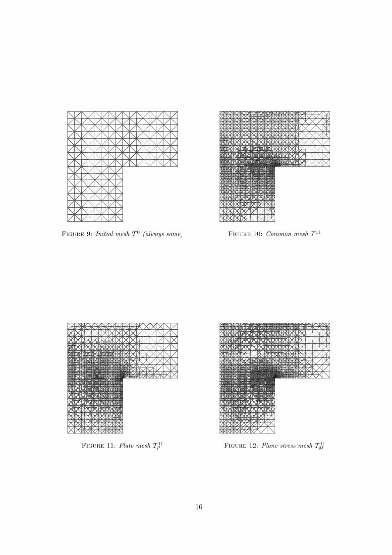
Figure 9: Initial mesh T 0 (always same) Figure 10: Common mesh T 11

Figure 11: Plate mesh T 11P Figure 12: Plane stress mesh T 11

M

16

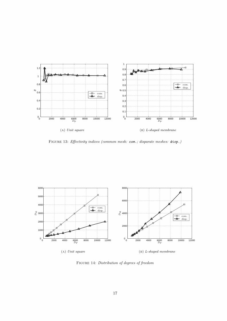
0 2000 4000 6000 8000 10000 120000

0.2

0.4

0.6

0.8

1

1.2

PSfrag replacements

DP

θ

com.

disp.

(a) Unit square

0 2000 4000 6000 8000 10000 120000

0.1

0.2

0.3

0.4

0.5

0.6

0.7

0.8

0.9

1

PSfrag replacements

DPθ

com.

disp.

(b) L-shaped membrane

Figure 13: Effectivity indices (common mesh: com.; disparate meshes: disp.)

0 2000 4000 6000 8000 10000 120000

1000

2000

3000

4000

5000

6000

PSfrag replacements

DP

DM

com.

disp.

(a) Unit square

0 2000 4000 6000 8000 10000 120000

2000

4000

6000

8000

PSfrag replacements

DP

DM

com.

disp.

(b) L-shaped membrane

Figure 14: Distribution of degrees of freedom

17

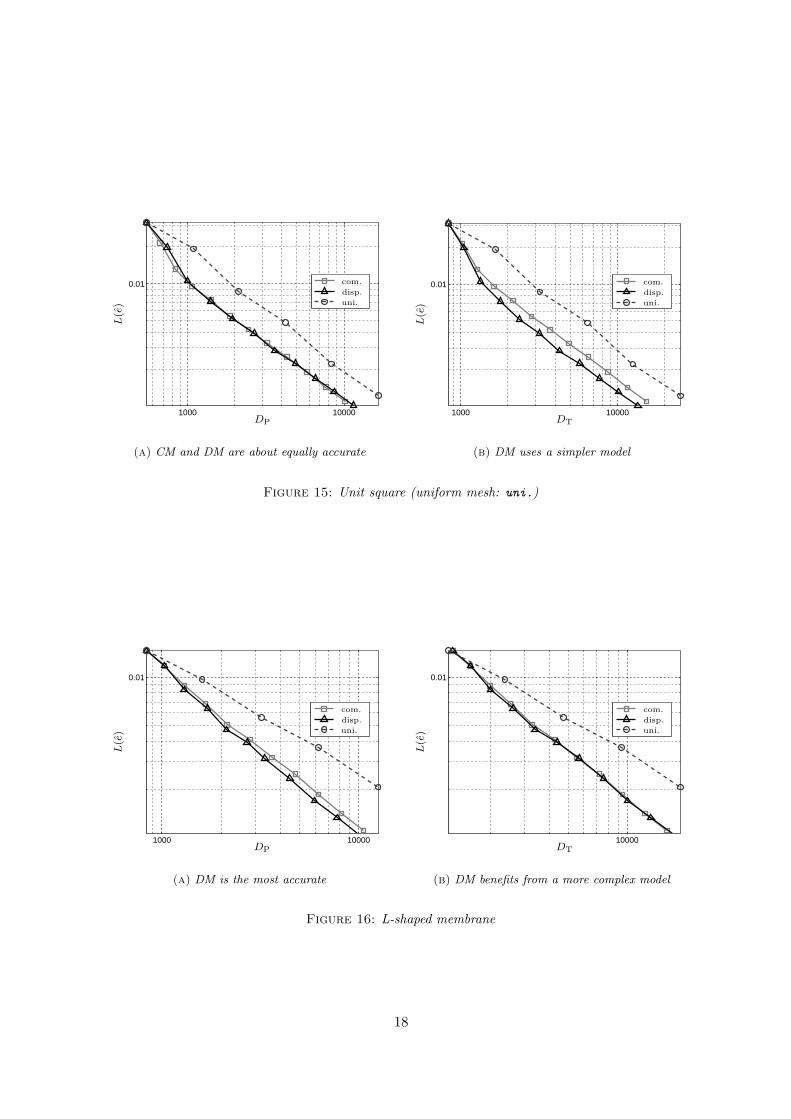
1000 10000

0.01

PSfrag replacements

DP

L(e

)

com.

disp.

uni.

(a) CM and DM are about equally accurate

1000 10000

0.01

PSfrag replacements

DTL

(e)

com.

disp.

uni.

(b) DM uses a simpler model

Figure 15: Unit square (uniform mesh: uni.)

1000 10000

0.01

PSfrag replacements

DP

L(e

)

com.

disp.

uni.

(a) DM is the most accurate

10000

0.01

PSfrag replacements

DT

L(e

)

com.

disp.

uni.

(b) DM benefits from a more complex model

Figure 16: L-shaped membrane

18

Model Adaptivity in Elasticity

Documents

Transcript of Model Adaptivity in Elasticity