Visa MasterCard incoming / outgoing Aplikacija VMC IT Sistemi .
Commun. math. Phys. 5, 23—41 (1967)
Mixture of Outgoingand Incoming Electromagnetic Radiation.Change of Mass of the Source of Radiation*
M. A. ROTENBERG, Ph.D.
The Negev Institute for Arid Zone Research, Beersheva, Israel
Received January 11, 1967
Abstract. In a previous paper the author, using a method of successive approxi-mations, verified by means of the Einstein-Maxwell equations of general relativitythe well-known result that outgoing electromagnetic radiation from a sourceconveys energy, so that the source loses gravitational mass corresponding to thisenergy. The purpose of this work is to show a similar result for the general case ofany mixture of outgoing and incoming radiation.
1. Introduction
From everyday use of electromagnetic waves it is evident that theycarry energy. Any source that emits them must lose energy. In a previouspaper (ROTENBERG, 1966) this was verified via a method of approxima-tion applied to the Einstein-Maxwell equations
Rik = -8πEik (1.1)
for free space, by investigating radiation from a simple source — anelectric dipole oscillating smoothly for a finite period. It was shown thatthe source suffers a permanent reduction of gravitational mass equal tothe total energy of radiation emitted. The result referred to outgoingwaves only; the present work sets out to show a similar result for anymixture of outgoing and incoming waves, having as the source (andreceiver) the electric dipole just mentioned.
The electric dipole is explained more clearly in section 2, and insections 3 and 4 the metric and method of approximation are described.The solution (obtained in section 5 for the dipole) of the wave equationfor the electromagnetic 4-potential is needed in section 6 to calculate theelectromagnetic energy tensor and the total flux of energy of electro-magnetic waves from the source. Finally, the main result, that thesource undergoes a secular variation in mass equal and opposite to thetotal flux of energy of electromagnetic radiation, is established in section 7.The more complicated calculations occur in two appendices, followed by athird appendix containing a notation connected with mixed, outgoing andincoming, radiation and used frequently in this paper.
* This work is included in a thesis submitted by the author (1964) to theUniversity of London for the degree of Ph.D.

24 M. A. ROTE N BERG, Ph. D. :
2. The Source
We shall consider an electric dipole which consists of two particles A
and B of equal, negligible mass -~r m and carrying equal and opposite
charges ±e; the particles are made to vibrate symmetrically along theaxis Oz (of a rectangular Cartesian coordinate system) about their mid-point 0, the origin. Let us specify the positions of A and B at time t by
JS= [0,0, -£(*)], (2.1)
where ζ(t) is any given bounded function of t which is (i) constant out-side the finite interval ^ ̂ t ̂ £2, (ii) single valued and has uniquederivatives of all orders in the interval ^ ̂ t ^ £2: thus the system issupposed to vibrate smoothly and only between times tτ and £2. Weassume that the arbitrary motion of the charged particles, described byζ(t), is caused by a mechanical device (such as a spring) of negligible mass,insulated from the charges (so that e — const.) and confined within afinite region near 0. Uniform motion of the charges is ruled out.
Finally, the oscillation of the two particles of the dipole may beregarded as partly the cause of the outgoing waves and partly the effectof the incoming waves : thus the system acts as a 'source and receiver' ofthe waves.
3. The Metric
For the source introduced in section 2 (which is axially symmetricabout Oz) we shall, following BOKNΌR (1959), employ the axi-symmetricmetric
ds* = —Adr* — r*(Bdθ* + sin2ΘC dφ2) + Ddt2: (3.1)
(r, θ, φ) are the spherical polar coordinates of the field-point P andA, B, C, D are functions of r, θ, t. This metric is the diagonalized formof the more genera] axi-symmetric metric
ds* = —Adr* — r2(Bdθ* + sin2(9(7 dφ2) +
+ D dt2 + 2rE dr dθ + 2F dr dt + 2rG dθ dt , (3.2)
E, F, G also being functions of r, θ, t.
4. The Method of Approximation
In section 6, the formula for the electromagnetic energy tensor EiJc
for the dipole of section 2 turns out to be a double-parameter expansionof the form
Eiκ-Σ Σ e'a'Stte) (4.1)p = 2 8=2
in terms of the constants e and a. The parameter e is the charge of theparticle A of the dipole as in section 2; the parameter a, having the

Change of Mass by Radiation 25
dimensions of length, is defined by
«/(*), (4.2)
where ζ(t) is given by equations (2.1) and f(t) is dimensionless. We shall,therefore, suppose that the metric tensor can similarly be expanded:
due consideration being given to the fact that gik refers to flat space-time.
The method of approximation to be employed here involves theexpansions (4.1) and (4.3) for the Eik and gίk. Inserting these expansionsin the field equations (1.1) and equating the coefficients of epas, we getwhat is to be called the (ps) approximation, namely, a set of second-order differential equations of the form
(ps) (ps^ (gr) (v*)
Φim(9iώ = Ψιm(9ik) + const. xEik. (4.4)(ps) (V^
In these, the Φlm are linear in gijc (and their derivatives); the Ψίm are(if)
nonlinear in gik (q 5g p — 2, r ̂ s — 2) (and their derivatives) known from(22)
previous approximations. Thus, apart from the expressions inEik, the (22)(22)
approximation contains only terms linear in gi k (and their derivatives)(PS)
the nonlinear expressions Ψίm in equations (4.4) do not appear in theapproximation. It is in the solution of this (22) approximation that therefirst appears a term representing a permanent change of gravitationalmass of the source equal and opposite to the total flow of energy ofelectromagnetic waves from the source (section 7). So our aim is to get anappropriate solution of the (22) approximation, which is achieved insection 7.
The solution of the (ps) approximation, the (ps) solution, is the
gik which satisfy equations (4.4).To conclude this section we form expansions for the coefficients of
the metric (3.1): in virtue of equations (4.3) they are
00 00
OO CΛ3
-gn = A = 1 + Σ Σc<
-g,2 = r*B = ̂ (1+2? £ e>
'=r 2sinWl + Σ
dlt = D = 1 + Σ ^
(ps) (ps) (ps) (ps)
A, B, C, D being functions of r, θ, t.
Σp= 2 β= 2
(4.5)

26 M. A. ROTENBERG, Ph. D. :
5. Solution of the Potential Wave Equation
For the derivation of a formula for the energy tensor Eik — and, in(22)
particular, for Ei k required in the setting up of the (22) approximation —
it is necessary to calculate the electromagnetic 4-potential φit
Consider first any isolated electrically charged distribution. It is
shown in EDDHSΓGTON (1924, § 74) that φt satisfies the equation1
Λ ;α 6 = 4π(J;-^), (5.1)
Jt being the 4- current, if we impose the condition
P-.t = 0 (5.2)
For weak fields, φk, E\ are small, so that, to the first approximation,
equation (5.1) reduces to
(5.3)
In Galilean coordinates equations (5.3) and (5.2) are the familiar wave
and gauge equations(5.4)
*<&,< = 0, (5.5)
where β^ = — 1, — 1, — 1, +1, terms of small magnitude of order higher
than the first being neglected; equations (5.4) and (5.5) are thus the
linearized forms of equations (5.1) and (5.2) in Galilean coordinates.
The Kirehhoff solution of equations (5.4) and (5.5), for the general case
in which the sources of the field simultaneously emit and absorb radiation,
is
φ^ocφl+βφl (α + / ? = ! ) , (5.6)where
m^ = /r*-V;(£,£,MTr*)^, eiJifi = Q. (5.7)
v
The notation in this form of solution is as follows: In equation (5.6),<-) <+)φi and φi represent respectively the retarded- potential and advanced-
potential solutions of equations (5.4) and (5.5) and correspond to the
radiation emitted from, and absorbed by, the sources of the field; α, β
are non-negative constants, which will be referred to as the strengths of
the emitted and absorbed radiation, respectively. In the first of equations
(5.7) the integration is taken over any fixed space volume V containing
all the sources of the field and r* is the distance of the point P(x, y, z),
1 In this paper a Latin index runs from 1 to 4, a Greek one from 1 to 3; thesummation convention applies to both types of index. A semicolon subscriptdenotes covariant differentiation, a comma subscript indicates partial differentia-tion.

Change of Mass by Radiation 27
contained by the space element dv = dx dy dz of integration, from the
field-point P(x, y> z) of interest; the second of equations (5.7), deducible
from equations (5.4) and (5.5), simply expresses the law of conservation
of Jt.Before applying the solution (5.6) and (5.7) to the dipole of section 2
it will be convenient to re-express the solution so that r occurs in place
of r*, r being the fixed distance OP. On applying the result to the source
and introducing the notation (4.2) we obtain the following (multipole)
expansion for the solution of equations (5.4) and (5.5) in terms of eas
(s = 1, 2, 3, . . .) (see appendix I); only the leading term of each non-
vanishing φi is written out explicitly:
(5.8)
£4 = 2ea cos^r-1/' + r~ 2/) + 0(eα2)
valid for r>max. |f|, where the notation (III.l) of appendix III has
been used for / (t).
6. The Electromagnetic Energy Tensor and the Flux of Energy
For the dipole the components of the 4-potential in spherical polar
coordinates are, on account of equations (5.8),
φi = —2eαr~1 cosθf' + 0(βα2),
A ' ' (6-1)
φ± = 2ea cosί^/—1/' + r~ 2 /) + 0(eα2)
The components of the electromagnetic force tensor for any source are
given by the formula
&ik= Φi,k — Φk,i; (6 2)for the dipole, the values of the non-zero covariant components in spherical
polar coordinates turn out to be
F12 = —F21 = 2eaamθ(f" + r-1/') + 0(eα2), 1
~ +0(eα2), (6.3)
r-2/) + 0(ea2),\
and the non-vanishing contravariant components are given in terms of
the covariant ones as2
Fi2 F21 __ r-zπ i Πίpπ^n — -V —- r a 12 -t- u(ea ,Jplί __ 7/^41 _-__//' I ( Ί ( f > r f 2 \ I /'β 4.̂
-t J- x 14 "T" yc-u/ y , r . \\j.~τj
2 Henceforth, the notation 0(epas) indicates a double power series in e and aconsisting of terms of orders epar(r ^ s) and eaar(q > p, r ̂ 0).

28 M. A. ROTENBERG, Ph. D. :
The formula for any source for the components of the electromagneticenergy tensor is
Fab. (6.5)
From equations (6.5), (6.3) and (6.4) we find for the non-vanishing Eilc\xιspherical polar coordinates the following expressions for our special source :
En = 2e2α2[r-V(7' '2 + /"2) + 2r-*s*(J'f" + /'/") -f
+ /-4{s2(/'2 + /' 2 + 277")-4e2/'2}~-
— (4 — 5s2) (2r~57/' -f r-672)] -f- <9(e2α3) , (6.6)
r-2J£22- 2e2α2[— r-2s2(/"2 — /"2) + 2 r ~ 9 s * ( f ' f " — /'/") +
(4 — 5s2) (2r-57/' + r~6/2)] + 0(β2α3) , (6.7)2 θ 2 (/ / ' 2 — / / / 2 )~ 2r-*s*(J'f" — f ' f " ) +
+ (4 — 3s2) (2r-57/7 + r-672)] + 0(e2α3) , (6.8)
2e2α2[r-2<s2(7''2 + / / / 2 ) + 2r-*8*(f'f" + /'7") +
+ r-*{βa(7'a + /' 2 + 2/7") + 4c2/'2} +
+ (4 — 3s2) (2r-57/7 + r-672)] + 6>(e2α3) , (6.9)
(2r-57/' + r-6/2)] + 0(e2α3) , (6.10)
+ r-4(7/" + 77') + r-577Ί + £ (eV) , (6.ιi)r-1^ - Se*a*sc[r-*f'f" + r-*(7/" + 77') +
+ r-5777] + 0(β2α3) , (6.12
where s = sinθ, c = cosθ.We now calculate the total flux of energy of electromagnetic radiation
from the dipole across a sphere S with centre 0 and radius R : on account ofequations (6.11) and (4.3) it is given by
] + 0(e2α3) (α + β = 1). (6.13)
The total energy flowing out of an infinite sphere, centre 0, is therefore
t»/•
(oc-β)e*a* f " * ( ξ ) d ξ + 0 ( e * a 3 ) (α + 0 = 1) . (6.14)

Change of Mass by Radiation 29
This, for the general case α φ /?, does not vanish since /" (|) φ 0, uniformmotion of the charges having been ruled out. Hence, provided the wavesare not stationary one expects a permanent variation in mass of theoscillating dipole, of an amount minus the value (6.14), to show up in the(22) approximation to the metric3. This is confirmed in the next section.
7. The Solution of the (22) Approximation. Change of Mass of the Source
The (22) approximation is equation (4.4) with p = s — 2 and with(22)
Ψim = 0; explicitly, for the metric (3.1) it becomes equations (II. 1) to(22) (22) (22)
(II.7) of appendix II in which the quantities P, Q, . . ., N on the rightare given by
(22) (22)
P = — 1
(7.1)
> (22) (22)
(22) (22) L = —16τr^12f) I A-τrr-2 Ή]V — J v / ί-/ X!/22 ' (22) (22)
(22) (22) M = iLQnJE^
H = lΌTtr S -1^33 , (22) (22)
(22) (22) N = -
S = —lβπfiu>
and equations (6.6) to (6.12).The complete solution of the (ps) approximation is given by equa-
tions (II.8) to (11.11). It contains six functions of integration η (r, θ),
σ (r, 0), χ (r, t), v (θ, t), τ (θ, t), μ (r, t), only one of which, χ (r, t), to begiven a non-zero value in order to satisfy the two requirements laid downin the paragraph containing equation (11.13) of appendix II. The key to
(ps)
this solution is the value of A satisfying the inhomogeneous waveequation (II.8), which is inserted here for convenient reference:
(PS) (PS) (ps) (ps)
' — f [(Lι + r~lL) — f (N11-\-r-lN1)dt]dθ-
— (ηi + r-^η] + f ((% + r-1 cΓi) dθ — (χl + r~^} - (7.2)
Obtaining an appropriate exact solution of the (22) approximation isextremely difficult: to avoid prohibitive calculations we shall derive asuitable approximate one satisfying the (22) approximation up to termsof order r~3, i.e. a solution such that its insertion back into the (22) field
3 From the expansion (4.3) it is clear that in Galilean coordinates the com-ponents tj. of the energy pseudo-tensor are of order e4α4. This should be sufficientto indicate that the energy of gravitational radiation accompanying electro-magnetic radiation from the dipole is of order e4α4 and so may be overlooked, asthe components E^ of the electromagnetic energy tensor for the dipole are of ordere2α2 only.

30 M. A. KOTENBERG, Ph. D. :
equations leads to the cancellation of terms up to order r~~ 3. The reason forthis step is as follows :
Suppose that the occurrence of electromagnetic waves is accompaniedby a secular variation in the mass of the source. Then the form of theSchwarzschild solution shows that for large r the coefficient of r~1in themetric for the dipole after the end of its oscillation should differ from thatbefore the beginning. It is therefore the r"1 terms in the solution of the(22) approximation that we are interested in, and they do not produceterms of order exceeding r~3 on the left of equations (II. 1) to (II. 7)(p = s = 2) . Hence we assume that it is sufficient to obtain a suitableapproximate solution of the (22) approximation (II. 1) to (II. 7) (p = s = 2)satisfying the latter up to terms of order r~3. In any case this will ensurethat up to the (22) approximation the total flux of 'phoney' matter acrossa large sphere with centre 0 and radius R (got by using the material energytensor Tik) is of order R~2, i.e. zero across an infinite sphere. Thus theapproximate solution and the corresponding exact solution of the (22)approximation should give the same numerical result as far as the totalvariation in mass of the source is concerned (cf. BONNOB, 1959, § 11 forthe case of gravitational waves).
In accordance with the above wre need values for the quantities (7.1)only up to terms in r~3: from the formulae (6.6) to (6.12) they are
(22) (22)
P=8 = -32πs2[r-2(/"2 + /"2) + 2r-3(/'/" + /'/")
\Δύ) __ __
L = 128πsc[r-2/'/" + r~3(fj" + / / 2)] ,
'"/" + r-8(7'7"+ /'/")]
-2/7" + r-3(//" + 77')
(22)
Jf =
(22)
^ = —
. (7.3)
It will save a great amount of work if the expressions (7.3) are eachbroken up into two parts, as below :
where
(22) (22) (22)
P = P + P , etc. ,1 2
(7.4)
(22) (22) (22)
= £ = Jf = 0,1 1 1
(22) (22) r , r ,
Q = —R = 64πs2(r-2 /"/ " — 2r-3/7 ) >, , r , , ,
2 C " - 8 " '(7.5)

Change of Mass by Radiation 31
(22) (22) ( - ) ( A )
P = S = — 64πs2(r-2/"/ " + 2r~3 J ' f " ) ,(22) (22)
Q = Λ2 2
(22) ,
i = 128πβc[r-»V7(22) ί- )
Λf -
Here, the notations (III. 2) and (III. 3), as applied to /, are assumed. The(22) (22) (22)
above treatment for P, Q, . . . , N automatically leads to a similarsplitting of equations (II. 1) to (II. 7) (p = s = 2) (which are linear in the
gijc and their derivatives) into two sets of equations (I) and (II), havingfor the right-hand sides the expressions (7.5) and (7.6), respectively.
Our object now is to obtain suitable approximate solutions of equa-tions (I) and (II) satisfj^ing them up to order r~3. To avoid possible
(22)confusion we shall distinguish the corresponding gik, occurring on the
(22) (22)left of equations (I) and (II), by designating them as gik and gik, respec-tively. x 2
The key equation (7.2) (p = s = 2) will now consist of two parts: bymaking use of the formulae (7.5) and (7.6) these become, up to order r~3,
52 /'/ " , (7.7)
2(-2 {]'f" + 7) - (7ι + r~^χ) (7.8)
in equation (7.8) the notation (III.7) has been used to introduce the
symbol Ϋ, where Y(ξ) is defined byΓ'(!) = X(!) = /"2(f). (7.9)
(22) (22) (22)In obtaining equation (7.7) we put all the arbitrary functions η , σ , χ
equal to zero, whereas in obtaining equation (7.8) we retained χ for uselater to preclude singularities from appearing along Oz (except at 0).
For a solution of equation (7.7) it is found necessary to proceed as far(22)
as the term of order r ~ 3 in the cal culation of A , if the corresponding complete
solution of equations (I) is to satisfy the latter up to order r~3.4 Forequation (7.8), however, the situation is somewhat different. It turnsout that, to obtain a solution of equations (II) satisfying them up to
(22)
order r~3, it is sufficient to solve equation (7.8) for A only to order(22) (22) (22)
r~l. In the expressions for B, C, D, found with the aid of equations (II. 9)4 This solution of equations (I) will itself contain only terms of order r~2 or
higher, as we shall soon find (see the solution (7.11)), and will accordingly be neg-lected in due course.
32 M. A. ROTEKBERG, Ph. D.:
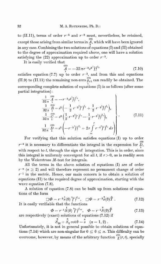
to (11.11), terms of order r~2 and r~3 must, nevertheless, be retained,(22)
except those arising froin similar terms in A, which will have been ignored
in any case. Combining the two solutions of equations (I) and (II) obtainedto the degree of approximation required above, one will have a solutionsatisfying the (22) approximation up to order r~3.
It is easily verified that(22) , _ ,
A Q9τr^— 3 o2 44 ' CJ I A\jπi — dΔTl Γ & I I I / . J.U ii / ; v '
satisfies equation (7.7) up to order r~3, and from this and equations
(II.9) to (11.11) the remaining non-zero gik can readily be obtained. The1
corresponding complete solution of equations (I) is as follows (after somepartial integration):
-J_7___ -3 2 [ 7/ ] >32π i ~~ T S '' '
32τr
(7.11)32π
1 <22> / [ ] / [ ]. Γ) __ Q2 I r-3 / / ' 4_ 9r / r-4 /' / ' dr32π r~ 5 \-r ft +2TJ T f f dT,
\ 00 /
For verifying that this solution satisfies equations (I) up to order(22)
f~3 it is necessary to differentiate the integral in the expression for Z),
with respect to t, through the sign of integration. This is in order, sincethis integral is uniformly convergent for all t, if r > 0, as is readily seenby the Weierstrass Jf-test for integrals.
All the terms in the above solution of equations (I) are of orderr~n (n ̂ 2) and will therefore represent no permanent change of orderr"1 in the metric. Hence, our main concern is to obtain a solution ofequations (II) to the required degree of approximation, starting with thewave equation (7.8).
A solution of equation (7.8) can be built up from solutions of equa-tions of the form
It is easily verifiable that the functions
Φ = r-* S(θ) (J'f", Φ = r-lS(θ)f (7.13)are respectively (exact) solutions of equations (7.12) if
S22 + S2cotθ = s ( α = l , 2 ) . (7.14)Unfortunately, it is not in general possible to obtain solutions of equa-tions (7.14) which are non-singular for 0 ̂ θ ̂ π. This difficulty can be
overcome, however, by means of the arbitrary function χ (r, t), specially

Change of Mass by Radiation 33
retained in equation (7.8) for this purpose. Consider then the equations
(22)
and choose χ (r, t) such that(22) , τ<22) q < l / A / 7 Q£ /rr i t f \Zi + r-1* = &ι?-3/7 > V~3^ (7 16)
in the first and second wave equation, respectively. Employing again thefunctions (7.13) in equations (7.15) gives
£22 + S2 cotθ - s — ka (α = 1, 2) (7.17)instead of equations (7.14), and suitable values for the constants k± andk2 can be found so that equations (7.17) possess non-singular solutions for0 ^ θ ̂ π.
By this method we can obtain a solution of equation (7.8) (see below),(22)
non-singular in θ, with χ (r, t) satisfying1 (22) (22) / 8 <-.,*>„ 4 .£\
32^- ( *ι + ̂ % ) = *-* (- y /'/ + -3 Γ) - (7-18)(22) <22> <22> (22)
For the remaining non-zero gίjc the values of B, C, D can now be2 2 2 2
calculated up to order r~3 by means of equations (II. 9) to (11.11). It must(22)
be emphasized at this stage that the function χ, satisfying equation(22)
(7.18), occurs again in the formula (11.11) for D. With the remaining
functions of integration put equal to zero, a complete solution of equations(II) is found in the above manner to be (after several partial integrationsare carried out)
-1 f r~ *']'?' dr\ ,J I
!_^_,2/ lr-ιW»32π V ~ ' Q ' '
(7.19)
3 Commun. math. Phys., Vol. 5

34 M. A. ROTENBERG, Ph. D.:
where the notation (III.5) has been employed for the introduction ofX, X ( ξ ) being defined by the second equality of (7.9). In the veri-fication that this solution satisfies equations (II) up to order r~3 it isnecessary to differentiate various integrals with respect to t through thesign of integration. This is allowed on account of the fact that thoseintegrals are uniformly convergent for finite t when r > 0, as can beshown immediately by the Weierstrass Jf-test.
Combining the two solutions (7.11) and (7.19) of equations (I) and(II), respectively, we obtain, as a suitable solution of the (22) approxi-mation satisfying the latter up to terms of order r~3,
(7.20)
32 π
Here, EA, . . ., RD (which, incidentally, together include all the terms ofthe solution (7.11) of equations (I)) consist entirely of terms each of whichis either of order r~2 or higher for all t, or of order r-1 and tends to zeroas ί-> ±°°; so BAί . . . do not contribute to any permanent change oforder r~1 in the metric.
This solution (7.20) is difficult to interpret physically. However, thecoordinate transformation
θ = (9* X
i t y , <*) dη + ~ ,t*)dη\,
,
[r* -j
Γ(r*, ί*) + r* f η-1 t(η, t*)dη\,CO J
(7.21)

Change of Mass by Radiation 35
where s* = sinθ*, c* = cosθ* and the notations (III.5) and (III.7) applyto X ( ξ ) and Y(ξ) of (7.9), brings it to one that can be physicallyinterpreted as we shall soon find. The transformed (22) solution is
32 π 32 π
(22)
A
32 π
132 π C =--^
1 <22> 1
32 π
32 π
Ί
1 , (22) 1 <2J>
r-1 a =32 π 32 π
(7.22)
[r r -|
y y T^-1! (η, t) dη + y r f η~*ί (η, t)dη\,
00 00 J
the asterisks being omitted the previous approximations are unaffected.During the transformation it is necessary to differentiate some of theintegrals in equations (7.21) with respect to t through the sign of inte-gration. This is permissible, since the Weierstrass M-test can be used toshow that these integrals are uniformly convergent for finite t, if r > 0.Involving the same method of differentiation is the verification thatthe solution (7.22) satisfies up to order r~3 the (22) approximation for thenon-diagonal metric (3.2), i.e. equations (11.14) to (11.20) with the right-hand sides given by the formulae (7.3), when appropriate values forRA, . . ., ED are used in the process.

36 M. A. ROTENBERG, Ph. D.:
In examining the solution (7.22) for physical interpretation we noticeintegrals of the types
fη-ιX(η,t)dη, f η-*X(η,t)dη , (7.23)
where X(r, t) stands for X or J?. It is easily shown that these exist forall r > 0 and all t that for any given finite value of t these tend to zero asr->σo at least as rapidly as r~2 and r~3, respectively; that, from theWeierstrass Jf-test, these are uniformly convergent for —σo < t < oo,for any given positive value of r. As t -> i °°5 the integrals (7.23) tendto zero (at least as rapidly as t~l and t~2, respectively), as can be seenqualitatively by regarding X(t =F η) as a (5-function; a similar argumentshows that they tend to zero as r tends to infinity with \t\ in such a waythat t =f r -> a finite limit.
It follows that the metric (7.22) possesses no singularities for r > 0.Moreover, owing to the fact that, as r -> oo and t -> i σo, the derivativesof the expressions (7.23) tend to zero at least as rapidly as the expressionsthemselves (this becomes obvious on differentiation), it follows that themetric (7.22) tends to flatness as r -> oo and t -> ± σo.
Ignoring the expressions (7.23) and RA, . . ., ED in the solution (7.22),which do not give significant changes in the metric, the solution becomes
64 nΛ -A 64 π
~l Y = —7Γ- r~ a*ff"*(ξ)dξ-β*ff"*(ξ)dξ\ (7.24)
according to the notation (III.7) and equations (7.9). If r(>0) is given,then
(2 1 : (22)
£ll = #44
64 π
64 π
, lor t <c t-^ — T ,
ί. (7-25)
f " * ( ξ ) d ξ , for t>t2 + r.
The formula (7.25) corresponds to an approximate Schwarzschild metric(with terms in r~2 ignored) for a single uncharged particle of mass mgiven by
32 π
, for t < t l - r ,
, for t > t2 + r .
(7.26)
Change of Mass by Radiation 37
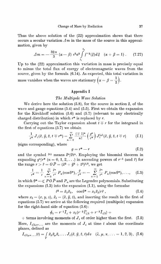
Thus the above solution of the (22) approximation shows that there
occurs a secular variation Am in the mass of the source in this approxi-
mation, given by«.
OO _ /•
(α + β = 1) . (7.27)
Up to the (22) approximation this variation in mass is precisely equal
to minus the total flux of energy of electromagnetic waves from the
source, given by the formula (6.14). As expected, this total variation in
mass vanishes when the waves are stationary loc=β = —\.
Appendix I
The MuUipole Wave Solution
We derive here the solution (5.8), for the source in section 2, of the
wave and gauge equations (5.4) and (5.5). First we obtain the expansion
for the Kirchhoίf solution (5.6) and (5.7) (relevant to any electrically
charged distribution) in which r* is replaced by r.
Carrying out the Taylor expansion about t T r for the integrand in
the first of equations (5.7) we obtain
n = 0 '
(signs corresponding), where
g = r*-r (1.2)
and the symbol W means dnldtn. Employing the binomial theorem in
expanding gw/r* (n = 0, 1, 2, . . .) in ascending powers of r~l (and r) for
the range r > r = OP = (x2 + y* + έ2)1/2, we get
^=~ Σ £Pn(cθS0*), £ = - Σ -^-Pn(θOBθ*), . . . , (1-3)n=Q n=l
in which θ* = < POP and Pn are the Legendre polynomials. Substituting
the expansions (1.3) into the expansion (I.I), using the formulae
r2 = x^Xχ, cosθ* = xλxλjrr , (1.4)
where Xχ — (x, y, z), Xχ— (x, y, z), and inserting the result in the first ofequations (5.7) we arrive at the following required (multipole) expansion
for the right-hand side of equation (5.6) :
φt = r-U, + xλ(r-*ϊ'ilλ + r-3/,/Λ) +
H- terms involving moments of J^ of order higher than the first. (1.5)
Here, I i / ^ μ V m m . are the moments of Ji at time i about the coordinate
planes, defined as
Ii/λμv...(t) = fxλxμxv. . .J^x.y.z.^dv (λ,μ,v,... = 1,2,3), (1.6)v

38 M. A. ROTENBERG, Ph. D.:
and the notation (III.l) of appendix III has been used. In this solutionthe expansion is valid for any point on or outside the smallest sphere,centre 0, that can enclose for all time all the sources of the field.
For the particular system of section 2 we use the notation (4.2) toobtain readily the solution (5.8), valid for r > max. |f|. This is the re-quired solution for this source, because it satisfies the gauge equation (5.5)as well as the wave equation (5.4) — an expected result since equation(5.5) implies and is implied by the second of equations (5.7), i.e. β = const.,for any φi satisfying equation (5.4) (HOLLER 1962, § 55).
Appendix II
The Approximate Field Equations and their Solution
The (ps) approximation for the diagonal metric (3.1), which is thecoefficients of e^a8 obtained on insertion of the expansions (4.5) and (4.1)in the field equations (1.1), is written out below. To save printing thelabels (ps), which should have been inscribed above the capital letters,have been omitted throughout this appendix, except for those fewplaces where confusion might arise without them.
2R'n - 0: —An + Bn + Cn + Dn + 2r-1(~A + B± H- Cx) +
-f r-*(A22 + A2 cotθ) - P , (Π.l)
2r-*R'22 = 0: Bn — 544 + r~l(—A1 + 3B1 + C1 + D1) +
-f r-*(A22 — 2A — B2eotθ + 2B +
+ C22 + 2C2 GotO + E>22) = Q , (11.2)
2r-25-2^3 = 0: Cu~ (744 + r~^(~AI + B1 + 3Cί + A) +
+ r-2ς42cotθ — 2A — B2 cotθ -f 2J5 + C22 -f
+ 2C2 cotθ + D2 cotθ) = R , (II.3)
2R'U = 0: J.44 + 544 + 044 — Dn — 2r-1D1 —
— r-2 (D22 + D2 cot θ) = 8 , (II.4)
2^ί2 - 0: —Bl cot θ + CI2 + GI cotθ + D12 —
— r~l(A2 + D2) = L, (II.5)
2R'U = 0: BU+ C14 + r-i(-2Az + B^ + <74) = M , (II.6)
2^4 - 0: ^24— 54 cotθ + 0>4 + 04 cotθ - N , (II.7)
where R'ik = ^?z-7c + SπEΪJC. In the above equations a subscript 1,2 or 4after ^4, B, C or D indicates differentiation with respect to r, θ or £ —this is to apply to any non-tensorial symbol unless otherwise implied. Theleft-hand sides of the above equations, corresponding to the Φlm in
equations (4.4), comprise linear terms in gijc (and their derivatives);
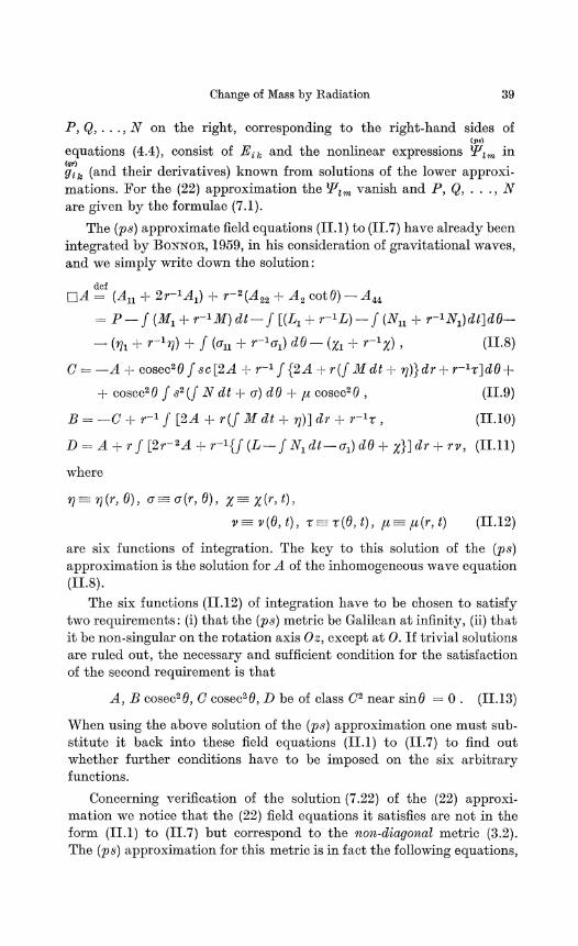
Change of Mass by Radiation 39
P,Q, . . ., N on the right, corresponding to the right-hand sides of(PS)
equations (4.4), consist of Eίk and the nonlinear expressions Ψΐm in(qr)
gik (and their derivatives) known from solutions of the lower approxi-mations. For the (22) approximation the Ψlm vanish and P, Q, . . ., Nare given by the formulae (7.1).
The (ps) approximate field equations (II. 1) to (II. 7) have already beenintegrated by BONNOB, 1959, in his consideration of gravitational waves,and we simply write down the solution :
=f (An 4- 2r-Mi) + r~*(A^ + A2 cotθ) — A^
= P — f(M1 + r-*M) dt — f [(Li + r-iL) — f(Nκ + r^N^d^dθ—
- (ηι + r-iη) + f (σu + r^aj dθ - (Xl + r^χ) , (II.8)
+ cosec2θ / s*(f N dt + σ) dθ + μ cosec2(9 , (II.9)
B = — C + r-1 f [2 A + r(f M dt + η)] dr + r~^τ , (11.10)
D = A + r f [2r~*A + r~^{f (L — f^ dt — σj dθ + χ}] dr + TV, (11.11)
where
η^η(r,θ), σ~σ(r}θ), χ=χ(r,t)9
v=v(θ9t)9 τ=τ(θ, ί ) , μ=μ(r9t) (11.12)
are six functions of integration. The key to this solution of the (ps)approximation is the solution for A of the inhomogeneous wave equation(Π.8).
The six functions (11.12) of integration have to be chosen to satisfytwo requirements : (i) that the (ps) metric be Galilean at infinity, (ϋ) thatit be non-singular on the rotation axis Oz, except at 0. If trivial solutionsare ruled out, the necessary and sufficient condition for the satisfactionof the second requirement is that
A, B cosec2θ, C cosec2θ, D be of class C2 near sinθ = 0 . (11.13)
When using the above solution of the (ps) approximation one must sub-stitute it back into these field equations (II. 1) to (II. 7) to find outwhether further conditions have to be imposed on the six arbitraryfunctions.
Concerning verification of the solution (7.22) of the (22) approxi-mation we notice that the (22) field equations it satisfies are not in theform (II. 1) to (II. 7) but correspond to the non-diagonal metric (3.2).The (ps) approximation for this metric is in fact the following equations,

40 M. A. ROTENBERG, Ph. D.:
with P, Q, .. ., N having similar meanings as before:
+ 2r~i(—A1 + B1 + C1 + E12 + E± cotθ) +
+ r~z(A22 + A2 cotθ + 2E2 + 2E cotθ) = P , (11.14)
#11 ~ #44 + r~l(~^ι + 3B1 + Cl + D1 + 2E12 — 2F± — 2£24) -f
+ r-*(A22 — 2A — B2 cotθ + 2J5+ C22 +
+ 202 cotθ + ,D22 + 4^2 + 2E cotθ) = Q , (11.15)
C'u — ^44 + r-1(—A1 + B1 + 3C1 + D1 + 2E1 cotθ — 2P4 — 2(74 cotθ) +
+ r-2(^2cotθ — 2A~- ^2 cotθ + 2^+ (722 + 2^2 cotθ +
+ D2 cotθ + 2E2 + 4:E cotθ) = R , (11.16)
D2 cotθ) - 8 , (11.17)
— B1 cotθ + (712 + Ci cotθ
cotθ) —
L, (11.18)
4 + ίJ24 + J5J4 cotθ + G12 + ̂ cotθ) +
cotθ + G2+ G cotθ) - if , (11.19)
+ 3#4 + Jιa - 26?! + r(Eί
(PS) (P*) (Ps)
in which ,̂ P, G} coming from the expansions
(11.20)
00 00
012 =2 s = 2
00 00
= 2 s = 2oo oo
p = 2 s = 2
for the non-diagonal coefficients of the metric (3.2), have been included.
Appendix III
Notation Related to Mixed (Outgoing and Incoming) Radiation
The notations introduced below for the treatment of combined out-going and incoming radiation avoid considerable writing in section 7.
If {^(1)} is a class of functions connected with gravitational or elec-tromagnetic wave fields, then
ώ<Λ> = ocψW (t — r) — βψW (t+r) , 1 ^ ' '

Change of Mass by Radiation 41
where <n> denotes dnjdtn (n ̂ 0).
If ψ(ξ) and λ(ξ) are two members of {ψ(ξ)},
Furthermore, if
then
Σ =
Finally, if
then we write
It is worth noting that
dXdr dt
dXdr
dXdt
dYdr
dY dY dγ_ _dt
References
(III.2)
(III.3)
(IIL4)
(III.5)
(III.6)
(III.7)
a/ > a*, a/ > a*, a/ ' a^ a/ (J-*-*- °)
BONNOB, W. B.: Phil. Trans. Roy. Soc. A, 251, 233 (1959).EDDINGTON, A. S.: The mathematical theory of relativity. Cambridge: Cambridge
University Press 1924.MOLLER, C.: The theory of relativity. Oxford: Oxford University Press 1962.ROTENBERG, M. A.: Gravitational and electromagnetic waves in general relativity.
London University Ph. D. thesis 1964.— Proc. Roy. Soc. A, 293, 408 (1966).