Scattering Tutorial

Erich Mueller

August 12, 2002

This tutorial is derived from an appendix to my thesis (http;//www.physics.ohio-state.edu/~emueller/thesis). It covers the standard physics of low-energy s-wave scattering as found in textbooks [1]. It attempts to be peda-gogical. See http;//www.physics.ohio-state.edu/~emueller/scatter forsupplementary Java programs.

1 The Scattering amplitude

1.1 Definition

The basic picture of potential scattering is illustrated in Fig. 1. One has anincoming wave eikz that is incident on a small impurity of size r0 (positioned atthe origin), and one asks what the far field wavefunction looks like. Generically

ψ(r) = eikz + f(k, r)eikr

r, (1)

which has the form of the incoming wave plus a scattered wave. In the far fieldr r0, the scattering amplitude f can only be a function of the incident wavevector k, and on the direction r. (In this equation f is also implicitly a function

of the direction of the incoming wave, generically denoted k and here set to z.For a spherically symmetric potential f is independent of k.)

In the long wavelength limit kr0 1 one expects that the scattering willbecome isotropic – the wave is too large to “see” the structure of the impurity.Thus one can drop the r dependences and only consider f(k), referred to asthe s-wave scattering amplitude. All of our discussions will be limited to thiss-wave limit. The same argument implies that f does not have much momentumdependence. For the most part this statement is true and f can be replaced byf(k = 0); however in the presence of a scattering resonance, f depends stronglyon k. These resonances are of immense experimental importance.

It is worth mentioning that resonant scattering in higher momentum chan-nels (“shape resonances”), can lead to angular dependence of f in the longwavelength limit. These resonances play no roles in current alkali gas experi-ments.

1

e ikz

Incoming Wave Outgoing Wave

e ikr

r

Figure 1: Generic Scattering Geometry. An incoming plane wave eikz reflectsoff a small impurity.

1.2 T -matrix

There are two problems in scattering theory. First, relating the scattering am-plitude to the scattering potential, and second, relating the properties of thesystem to the scattering amplitude. The first problem amounts to solving theSchrodinger equation in the presence of the impurity, with the boundary condi-tion that the incoming wave is eikz . Generically solving this equation requiresthe use of computers, but in principle is solvable to arbitrary precision.

As an alternative to computers, one can also use perturbation theory to solvethe Schrodinger equation. For realistic atomic potentials perturbation theoryis not going to work well. Nevertheless it is still useful to formally develop thescattering amplitude as a sum of terms, each one containing higher powers ofV . One can then think of the scattered wavefunction as coming from multiplescattering from the impurity.

The standard approach to developing the perturbation series is to write theSchrodinger equation in integral form. Formally I write

ψ = φ− 1

H0 −EV ψ, (2)

where φ = eikz is the incident wave function, V is the scattering potential,E = k2/2m is the energy of the state, and (H − E)−1 is the Green’s functionfor the free Schrodinger equation. Applying H0 −E to Eq. (2), one arrives at

(H0 −E)ψ = −V ψ, (3)

which is the conventional Schrodinger equation.As can be verified directly, in momentum space and in real space, the Green’s

functions are given by

〈q| 1

H −E|q′〉 =

(2π)3δ3(q − q′)

q2/2m−E(4)

2

〈r| 1

H −E|r′〉 =

m

2π

exp(ik|r − r′|)|r − r′| , (5)

where E = k2/2m. On physical grounds, I have chosen outgoing boundaryconditions in Eq. (5). This latter result is only true in three dimensions. Gettingaway from my schematic notation, one writes Eq. (2) in one of two forms,

ψ(k′) = (2π)3δ3(kz− k′)− 2m

∫

d3q

(2π)2V (k′ − q)

q2 − (k′)2ψ(q), (6)

ψ(r) = eikz − m

2π

∫

d3r′eik|r−r

′|

|r− r′| V (r′)ψ(r′), (7)

The first equation is in momentum space, the second in real space. In thisSection I only consider the real space equation (7), though later I will focus on(6). For simplicity I assume that V (r) falls off over a lengthscale r0. Longerrange potentials can be treated, but such analysis is not particularly importantfor discussing neutral atoms.

In the far field, r r0, one can expand the difference |r− r′| in the integral,to arrive at the equation

ψ(r) = eikz − m

2π

eikr

r

∫

d3r′ eikr·r′

V (r′)ψ(r′). (8)

Comparison with Eq. (1) gives an expression for the scattering amplitude,

f(k, r) = −m

2π

∫

d3r′ eikr·r′

V (r′)ψ(r′). (9)

One generates a perturbative solution to Eq. (7) by a simple iterative scheme.One starts by setting ψ(r) = eikz on the right hand side of (7). This first orderresult is known as the Born approximation to scattering. This procedure isiterated by substituting the new value of ψ into the right hand side. In aschematic notation, one has

ψ =

(

1− 1

H0 −EV +

1

H0 −EV

1

H0 −EV +

1

H0 −EV

1

H0 −EV

1

H0 −EV + · · ·

)

φ.

(10)This expression is compactly written as

ψ = ψ0 −1

H0 −ETψ0, (11)

where the T-matrix is defined by

T = V + V1

H0 −EV + V

1

H0 −EV

1

H0 −EV + · · · (12)

= V + V1

H0 −ET. (13)

3

= + + ...+

= +

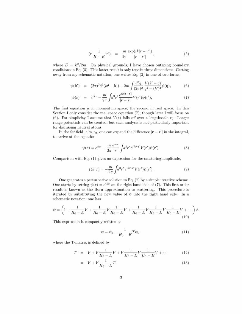
Figure 2: Diagrammatic representation of the T-matrix equation. The T-matrix, designated by a dark dashed line connected to an “X”, comes frommultiple scattering off the potential. The soft dashed lines represent bare po-tential scattering.

A diagrammatic representation of Eq. (12) is shown in Fig. 2. The scatteringamplitude is then related to the on-shell T-matrix, by the expression

f(k) =−m2πh2T (k). (14)

For the many-body problem, or for the problem of scattering off many impuri-ties, one in principle needs the off shell T-matrix.

To fully appreciate the structure of the T-matrix, one must go beyond s-wavescattering, and consider the generic scattering amplitude f(k, r, k) defined bythe asymptotic form

ψ(r) = eik·r + f(k, k, r)eikr

r. (15)

The scattering amplitude is a function of the direction of the incoming wave k,the direction of the outgoing wave r, and the energy of the scattering particle,k2/2m.

The T -matrix similarly is a function of three variables,

T (k,k′, q) ≡ 〈k′|T (E = q2/2m)|k〉 (16)

= 〈k′|V |k〉+ 〈k′|V 1

H0 −ET |k〉. (17)

The variables are the incoming momentum k, the outgoing momentum k′, andthe energy E = q2/2m. If one sets |k| = |k′| = q, one finds

f(k, k, r) = −m

2πT (kk, kr, k). (18)

The off mass shell terms of T give information about the non-asymptotic behav-ior of the scattering. If one throws away all this information, such as one does inthe pseudo-potential approximation, one finds that the T -matrix is independentof the momenta k and k′, and is only a function of the energy q

T (k,k′, q) = T (q) =−2π

mf(q). (19)

This approximation will clearly break down when the momenta are of atomicdimensions.

4

1.3 Phase shifts

In the limit of s-wave scattering, the impurity only sees the part of the incomingwave that is spherically symmetric. One finds the spherically symmetric part ofthe incoming wave by integrating over the solid angle,

∫

dΩ

4πeikz =

1

2

∫ 1

−1

d cos θ eikr cos θ (20)

=sin(kr)

kr. (21)

This wave has components which are propagating towards and away from theimpurity, as is seen by representing the wavefunction as

sin(kr)

kr=−1

2i

e−ikr

kr+

1

2i

eikr

kr. (22)

The scattering can only affect the outgoing wave. Since particles are conserved,the only possible change it can make to the outgoing wave (in the asymptoticregion) is to provide a phase shift, δ,

eikr → ei(kr+2δ) = eikr + 2ieikreiδ sin δ. (23)

Thus, in complete generality, one can write the scattered wavefunction as

ψ(r) = eikz +eiδ sin δ

k

eikr

r. (24)

Comparing with Eq. (1) one arrives at an expression for the scattering amplitudein terms of the phase shift.

f(k) = eiδ sin δ/k. (25)

1.4 Meaning of the scattering amplitude and the phase

shift

On a microscopic level, δ has a clear meaning. It is the phase shift of the scat-tered wave, relative to what it would be without the impurity. In the followingsection I will show how this phase shift can be simply related to the densityof states in the presence of the impurity. The scattering amplitude, f , is theamplitude that the particles are scattered. That is, σ = 4π|f |2 is the numberof scattered particles per unit flux of incoming particles. The cross section σ isthe area that a classical target would have to have for the scattering probabilityto be the same.

An equivalent way to understand f is to look at the equation

ψ = eikz + feikr

r. (26)

The length f gives the distance from the impurity at which the flux of scatteredparticles equals the flux of incoming particles.

For small δ Eq. (25) can be expanded, and one finds that f ≈ δ/k.

5

2 Relationship of the scattering problem with

the standing wave problem

In elementary quantum mechanics, the first problem one learns to solve is the“particle in a box.” One takes the Hamiltonian −h2∇2/2m, diagonalizes it viaa Fourier series, and finds the complete spectrum. Later one learns how to doscattering problems, where one is not interested in the spectrum (which is con-tinuous), but rather on transmission and reflection amplitudes. The relationshipbetween these two problems is rarely completely clear.

One can connect the scattering problem and the standing wave problem bylooking at scattering in a finite size box. The three dimensional case (whenlimited to the s-wave channel) is actually simpler than the one dimensionalproblem, so I will concentrate on it. I first “solve” the standing wave problem.Consider a small impurity with a potential V (r) in the middle of a big sphericalbox of radius R. I wish to find the eigenvalues of the Schrodinger equation,

[−∇2

2m+ V (r)

]

ψ(r) = Eψ(r), (27)

with the boundary condition that ψ(R) = 0. I take h = 1, and restrict myselfto spherically symmetric states. By substituting ψ(r) = u(r)/r, one can writes-wave sector of the Schrodinger equation as

[−1

2m

d2

dr2+ V (r)

]

u(r) = Eu(r), (28)

with the boundary condition u(0) = u(R) = 0. For r larger than the range of thepotential, one can ignore V (r), and this equation is just a free one dimensionalSchrodinger equation. Thus in the asymptotic regime there is some δ such thatthe solution to (28) is u(r) = sin(kr + δ). To satisfy the boundary conditionsthe momentum k must obey kR+ δ = nπ, for some integer n.

Now imagine one performs a scattering experiment on the same potential.One sends in a wave u(r) ∼ e−ikr , and looks at what comes out. Thus one mustsolve Eq. (28) with the condition that the incoming part of u is (−1/2i)e−ikr.Well, we know one solution of Eq. (28), which asymptotically is u(r) = sin(kr+δ). Multiplying by −2ieiδ, one gets u(r) = e−ikr − eikre2iδ . Since solutions tothe Schrodinger equation with a given boundary condition are unique, this umust be the scattered wavefunction. Comparing with Eq. (23), one sees thatthe δ which arises in solving the standing wave problem is the same as the δwhich appears in the scattering problem. With this relationship one can solvethe scattering problem by using the powerful computational techniques whichhave been developed for ground-state problems (see for example [2]).

2.1 Energy shifts

The relationship between scattered states and standing waves gives rise to avery nice graphical construction which allows one to relate the density of states

6

δ

0

−π

kRπ 2π 3π 4π 5π 6π 7π

kR+ =nδ π

Figure 3: Connecting phase shifts and energy shifts. The thick line representsthe phase shift δ(k). In a box, sin(kR + δ) = 0, so the allowed states lie at theintersection of the thick line and the oblique lines kR + δ = 0. As the box ismade larger, the spacing between the oblique lines becomes smaller, and (on anabsolute scale) they become more perpendicular to the k axis.

to the phase shifts. Imagine one knows the phase shifts δ(k) (for example, seeFig. 3). If one places the system in a box, the only states which obey theboundary conditions have kR + δ = nπ for some integer n. Thus the allowedstates have a wave vector given by the intersection of the lines kR+ δ = nπ andδ(k).

In the absence of an impurity the wave vectors allowed have kR = nπ. Thusthe shift in wave vector is δk = −δ/R, and the change in the energy of a state isδE = k δk/m = −δ k/mR, which is proportional to δ. As a historical note, thisresult was a point of confusion in the 1950’s in the context of the many-bodyproblem [3].

In the limit of large box, it is more convenient to talk about a density ofstates, rather than the energy of any particular state. Starting from the relationkR+ δ = nπ, one finds that the density of s-wave states in k-space is

∂n

∂k=R

π+δ′(k)

π, (29)

where δ′(k) is the derivative of δ with respect to k. The first term is the standarddensity of states in a 1-dimensional box, while the second term is the changein the density of states due to the impurity. Thus one interprets δ/π as thenumber of extra states with momentum less than k due to the impurity.

If one knows the density of states, then one can calculate For example,consider a spherical “bump” potential as depicted in Fig. 4. The bump has

7

V(r)

q2

2m

r

Figure 4: Energy states for a spherical bump in a box. States are pushed up bythe bump

Rπ

DOS

kq

R-rπ

Figure 5: Density of states for a spherical bump in a box (schematic). Thepotential has a height of V0 = q2/2m, and width r.

radius r0 and height q2/2m. For k q, the bump appears to be an infinitebarrier, and the density of states should be ∂n = (R − r0)/π ∂k, which is lessthan the density of states in the absence of the bump. The missing states haveto go somewhere, and they are pushed to momenta near k = q. For k q,the bump is irrelevant, and the density of states should be that of a free gas,∂n = R/π ∂k. One should therefore see a density of states like the one in Fig. 5.After integrating this curve, one arrives at a phase shift δ like the one depictedin Fig. 6.

As a corollary to the theorem that δ(k)/π is the number of extra states, onehas the general result that for a sufficiently well-behaved potential the k = 0the phase shift is equal to π times the number of bound states. Genericallyδ(k →∞) = 0, and the bound states are missing from the continuum.

8

kq

δ

Figure 6: Phase shift for a spherical bump in a box (schematic). The height ofthe potential is q2/2m.

3 Sample phase shifts

In this section I plot a few illustrative phase shifts.

3.1 Hard wall

The simplest scattering potential is a hard wall:

V (r) =

∞ r < r00 r > r0.

(30)

The wavefunction must vanish at the edge of the wall, so u(r) = sin(k(r − r0))and δ = −kr0. This example is pathological in that δ →∞ as k →∞.

3.2 Attractive well

A slightly more complicated simple potential is the attractive spherical well,

V (r) =

−V0 r < r00 r > r0.

(31)

This potential is not realistic but it possesses many of the features of moresophisticated atomic potentials. In particular there are low energy resonanceswhenever a new bound state enters the well. To find the phase shifts I writethe wavefunction as

u(r) =

A sin(k′r) r < r0B sin(kr + δ) r > r0,

(32)

where (k′)2/2m−V0 = k2/2m. Continuity of the wavefunction and its derivativeare guaranteed by matching the logarithmic derivative at r0, which gives

k′ cot(k′r0) = k cot(kr0 + δ). (33)

9

δ

k/π0.5 1 1.5 2 2.5 3

0.5

1

1.5

2

2.5

3

Figure 7: Phase shifts for a spherical well potential. The depth of the well isV0 = q2/2m and its radius is r0. All momenta are measured in terms of r0. Thevarious lines show different values of q, each differing by 0.1π/r0. Resonancesoccur at qr0 = (n+ 1/2)π.

Solving for δ gives

tan δ =k sin k′r0 cos kr0 − k′ sin kr0 cos k′r0k′ cos k′r0 cos kr0 + k sin kr0 sin k′r0

. (34)

For different values of V0 I plot δ(k) in Fig. 7. For simplicity I introduce themomentum q, satisfying V0 = q2/2m, which marks the depth of the well. Themost striking feature of these graphs is that when cos(qr0) = 0, the phase shiftat k = 0 jumps. This happens because a new bound state enters the well at thispoint.

It is instructive to put this system in a box of size R, and calculate theenergy of the first few levels as a function of q. As seen in Fig. 8, whenever onepasses through a resonance, the lowest energy state becomes bound, and thenext level replaces it. What is happening is that each line has a fixed numberof nodes, and at the resonance one of the nodes moves from outside the well toinside the well, drastically reducing the energy.

10

0.5 1 1.5 2 2.5 3Hr0ΠL q

2.5

5

7.5

10

12.5

15

H2mR2Π2L E

Figure 8: Energy levels for an attractive well of radius r0 and depth V0 = q2/2mwithin a box of size R. The energy is measured in terms of the quantizationenergy of the large box, π2/mR2. The horizontal axis shows qr0/π, a measureof the depth of the well. Resonances occur whenever qr0 = (n + 1/2)π, andone of the continuum energy states drops into the well. For this plot R = 50r0.Increasing R0 makes the jumps sharper.

11

V

r

q2

2m

r0 2r0

Figure 9: Resonant barrier potential.

3.3 Resonant barrier

I next consider a resonant barrier potential, as shown in Fig. 9,

V (r) =

0 r < r0q2/2m r0 < r < 2r00 r > 2r0.

(35)

As opposed to the attractive well which possesses zero energy resonances, theresonant barrier has finite energy resonances resulting from the quasi-boundstates which are found at momenta where sin(kr0) ≈ 0. At these resonances,one finds an extra state. From our understanding of δ′/π as the density ofstates, we should have a phase change of π near this momentum. As seen inFig. 10, this is indeed the case.

4 The pseudopotential

Here I discuss an expansion of the scattering amplitude in powers of kr0, wherer0 is the length scale of the potential. This expansion takes the form

k cot δ = − 1

as+

1

2rek

2 +O((r0k)4). (36)

The parameters as and re are known as the scattering length and the effectiverange. I emphasize that (36) is an expansion in r0k, and even when as is large,the remaining terms can be small. The pseudopotential approximation amountsto taking only the first term in this expansion.

One derives Eq. (36) via a matching argument. The Schrodinger equationobeyed by u(r) = rψ(r) is

(

k2 + ∂2r

2m− V (r)

)

u = 0. (37)

12

δ

k/π

0.5 1 1.5 2

-1

-0.8

-0.6

-0.4

-0.2

Figure 10: Phase Shifts δ(k)/π for a resonant barrier potential. The momentumk is measured in units of π/r0. Each line corresponds to a different barrierheight.

For r r0, V (r) dominates over k2, and one writes

u(r) = χ(r) +O(k2), r r0, (38)

where χ(r) is independent of k. For r r0, the potential V (r) vanishes and utakes on its asymptotic form

u(r) = A sin(kr + δ), r r0. (39)

I match the logarithmic derivatives at r0, finding

k cot(kr0 + δ) = χ′/χ+O(k2), (40)

which gives the desired expansion of k cot δ in powers of k2.In terms of cot δ the scattering amplitude is

f =eiδ sin δ

k=

1

k cot δ + ik. (41)

So in the pseudo-potential approximation, the scattering amplitude is

f =−a

1 + ika. (42)

For small ak, this looks like a point interaction. For large values of ak, thislooks like a long-ranged 1/k potential.

13

a/r

qr10 20 30 40 50 60

-2

-1.5

-1

-0.5

0.5

1

1.5

2

Figure 11: Scattering length a for a spherical well of radius r and depth V0 =q2/2m.

4.1 The pseudo-potential for an attractive spherical well

As an example, one can expand Eq. (34) in powers of k, finding

k cot δ =−1

as+rek

2

2(43)

as = r0 −tan qr0q

(44)

re = (1

q− r20q) cos qro + r0 sin qr0 +

q2r30 cos2 qr0/3

sin qr0 − qr0 cos qr0. (45)

The effective range vanishes when as diverges. These quantities are plotted inFig. 11 and 12.

5 Zero range potentials

For analytic calculations, the simplest potentials one can consider are zero-range potentials. These play an important role in many theoretical works, soit is worth considering them here. Zero range potentials are, by construction,singular. Thus, despite their analytic simplicity, these potentials require takingcareful limits.

14

re/r

qr20 40 60 80 100

-200

-100

100

200

300

400

Figure 12: Effective range re for a spherical well of radius r and depth V0 =q2/2m.

5.1 A structureless point scatterer

Consider a point scatterer with a potential V (r) = V0δ(r − r′). In momentumspace, Vk = V0. Scattering off this potential is described by the T -matrixequation (17),

Tkk′(ω) = Vkk′ (ω +∑

q

VkqG0(q)Tqk′ (ω). (46)

Since Vkk′ is independent of the momentum indices, T will also be independentof momentum. Using this result, the T -matrix is

T (ω) =V0

1− V0Θ, (47)

where Θ is given by

Θ =∑

k

G0(q, ω) =∑

q

1

ω − q2/2m. (48)

Replacing the sum with an integral,

Θ =V

(2π)3

∫

d3q

ω − q2/2m(49)

=V

2π2

∫

dq q2

ω − q2/2m, (50)

15

one notices that the sum is ultraviolet divergent. This divergence is a conse-quence of the short range of the potential, and reflects the fact that a pointinteraction is unphysical. Any real potential will have a finite range, which willintroduce a large q cutoff, Λ in this integral. The integral is readily evaluatedto be

Θ = Θ0 −imV

√2mω

2π(51)

Θ0 = −V mΛ

π2. (52)

The T -matrix is then of the form

T =2π

m

as

1 + ias

√2mω

, (53)

where the scattering length is

as ≡m

2π

V0

1− V0Θ0. (54)

Note that if one takes the cutoff Λ to infinity at fixed V0, then the scatteringlength vanishes. In this sense, there is no scattering off a delta-function potentialin three dimensions. Only by scaling V0 with Λ can a non-zero as be produced.This scaling of V0 with Λ is the simplest example of renormalization which canbe discussed. As previously discussed, a T -matrix of the form (53) gives a phaseshift

δ = arg(T ) = − arctan(ask). (55)

5.2 Scattering from a zero-range bound state

A simple generalization of the structureless point scatterer is to associate abound state with the impurity. In such a case, the scattering is energy depen-dent, and

Vk = V0 +|α|2ω − ε

, (56)

where V0 is a static potential at the origin, α is an amplitude for entering thebound state, and ε is the energy of the bound state. To illustrate the role of thebound state I set V0 = 0, in which case

T =|α|2

ω −E + i(m/2π)|α|2√

2mω. (57)

The energy E isE = ε+ |α|2Θ0. (58)

For E to be finite as Λ →∞ one must scale ε with Θ0.The T -matrix (57) leads to a phase shift of the form

cot(δ) = − 1

ask+ reffk

2/2, (59)

16

where

as =−m|α|2

2πE(60)

reff =−2π

m2|α|2 . (61)

A resonance occurs when E = 0.The Green’s function for the bound state is T/|α|2. Thus E is the energy of

the bound. When E > 0, this state has a finite lifetime

1

τ=m

2π|α|2

√2mE, (62)

which is the result one would expect from Fermi’s golden rule.

6 Feshbach resonances

As is clear from the above examples, tuning a resonance near zero energy hasdramatic consequences for atomic scattering properties. Experimentally suchtuning is carried out by applying magnetic fields. The field induced resonanceis known as a Feshbach resonance.

The underlying principle is that due to the hyperfine interaction, two collid-ing atoms can form a bound state whose magnetic moment is not equal to thesum of the magnetic moments of the incoming atoms (total angular momentumis conserved, not total magnetic moment). Consequently, when a magnetic fieldis applied, the Zeeman shift of the bound state can be different from the shiftof the scattering states. Thus the energy of the bound state is tunable. Whenits energy is set to zero one is at the resonance. The scattering properties nearthe resonance are described well by the model of Section 5.2.

7 Multiple scattering

I now turn to the question of scattering off several small impurities which aremuch farther apart than the range of their potentials. As detailed in Section 4,low energy scattering off an individual impurity is described by the scatteringlength as. Letting n denote the density of scatterers, I am particularly interestedin the limit where na3

s is of order 1. In this limit one encounters localizationeffects, and the scattering off of one impurity depends on the presence of allothers.

7.1 Elementary approach

In this Section I frame the problem in terms of elementary quantum mechanics.Imagine that one has static impurities at positions r1, r2, . . . , rn. The phase

17

shifts for scattering off any of these impurities is δ0(k). In a scattering experi-ment, the asymptotic wavefunction will be

ψ(r) = eikz +∑

i

fieik|r−ri|

|r − ri|, (63)

where the fi’s will be independent of space. This wavefunction should be good,except on atomic distances close to individual impurities. Comparing withEq. (1), the scattering amplitude for scattering from the collection of impu-rities is

f(k, r) =∑

i

fieikri ·r. (64)

The s-wave component of this scattering amplitude is

fs(k) =

∫

dΩ

4πf(k) =

∑

i

fisin krikri

. (65)

In particular, when kri 1 then

fs(k) =∑

i

fi. (66)

My goal is to calculate the phase shift δ given by

fs =eiδ sin δ

k. (67)

I now determine the fi’s via the restriction that at each impurity, the phaseshift is δ0. Once we know fi we know f . Near the ith impurity, the sphericallysymmetric part of ψ is defined by

ψ(s)i (|r− ri|) =

∫

dΩ′

4πψ(r = r′ + ri), (68)

where dΩ′ is a solid angle with respect to the variable r′, which is centered atthe impurity. The integration is straight forward and one finds

ψ(s)i (r − ri) =

eikzi +∑

j,j 6=i

fjeik|ri−rj |

|ri − rj |

sin k|r − ri|k|r − ri|

+ fieik|r−ri|

|r − ri|. (69)

I will use the symbol Ai for the term in large parentheses. We know that thisterm must have the form

ψ(s)i (r − ri) =

sin(k|r − ri|+ δ0)

k|r − ri|. (70)

Equating these two expressions, one arrives at

fi = Aieiδ0 sin δ0

k. (71)

18

Using this expression in the definition of Ai one finds that Ai satisfies thefollowing matrix equation,

(

δij − eiδ0 sin δ0eik|ri−rj |

k|ri − rj |

)

Aj = eikzj . (72)

I denote the matrix on the left hand side of this equation by 1 − g. Formallyinverting this matrix gives

A1

...An

=

1

1− g

eikz1

...eikzn

. (73)

The total scattering amplitude f is then

f(k, k, r) =eiδ0 sin δ0

k

(

e−ikr·r1 · · · e−ikr·rn) 1

1− g

eikk·r1

...

eikk·rn

(74)

=eiδ0 sin δ0

k

∑

ij

eik(k·ri−r·rj)

(

1

1− g

)

ij

. (75)

Formally we are now done. If kri 1 we neglect the eikri ’s and get

eiδ sin δ = eiδ0 sin δ0∑

ij

(

1

1− g

)

ij

. (76)

In this same approximation

gij =

eiδ0 sin δ0

k|ri−rj |i 6= j

0 i = j.. (77)

In the pseudo-potential approximation,

eiδ0 sin δ0 =−ask

1 + iask. (78)

It is useful to study the structure of (1−g)−1. The matrix g has the propertythat gij is a function only of the distance |ri−rj |, and is essentially a scatteringamplitude times a propegator. One graphically thinks of gij as a directed lineconnecting impurity i to impurity j. Then ((1−g)−1)ij is the sum over all pathsconnecting i to j.

7.2 T-matrix approach

With less work (but using more machinery) one can derive the results as thelast Section by directly calculating the T -matrix, defined by

T = V + V1

H0 −ET. (79)

19

In the present case, V =∑

i Vi is the sum of the potentials for each scatterer.If one defines Ti as the sum of scattering off an individual impurity,

Ti = Vi + Vi1

H0 −ETi, (80)

then T is given by a sum over all paths between scatters of Ti’s with propegatorsbetween them,

T =∑

i

Ti +∑

i6=j

Ti1

H0 −ETj + · · · , (81)

=∑

i

Ti +∑

ij

Ti(1− δij)1

H0 −ETj + · · · . (82)

I introduce a matrix Gij by

Gij = (1− δij)1

H0 −ETj , (83)

so that the T-matrix is formally

T =∑

ij

Ti

(

1

1−G

)

ij

. (84)

To go any farther one needs to choose a basis. The most convenient basisfor the current problem is in momentum space. If we treat the Ti’s within thepseudo-potential approximation, then

Ti(k, k′, q) = 〈k′|Ti(E = q2/2m)|k〉 = ei(k−k′)ri

(−2π

mqeiδ0 sin δ0

)

. (85)

For notational simplicity, I use the symbol x for the parentheses. The operatorTi(H0 −E)−1Tj is evaluated by inserting a resolution of the identity

〈k′|Ti(H0 −E)−1Tj |k〉 =

∫

d3k

(2π)3T (k, k, q)

2m

k2 − q2T (k, k′, q) (86)

= x2ei(krj−k′ri)m

2π

eiq|ri−rj |

q|ri − rj |. (87)

In Eq. (81) all of the eikri ’s cancel, except for the one at the end and the oneat the beginning. Thus T is given by

T (k, k′, q) = x∑

ij

ei(kri−k′rj)Mij(q), (88)

where Mij(q) is the sum of all paths going from i to j, each segment of the pathgoing from impurity µ to impurity ν contributing x(m/2π)eiq|rµ−rν |/(q|rµ−rν |),which is readily seen to be identical to (75).

20

7.3 Two scatterers

Given the positions r1, r2, . . . , rn of the scatterers we can now calculate δ interms of δ0. The simplest example of this procedure uses two scatterers. Thematrix gij is given by

g =

(

0 xx 0

)

(89)

x =eik|r1−r2|

k|r1 − r2|sin δ0e

iδ0 (90)

≈ −as(1 + ikr)/r

1 + ikas, (91)

where r ≡ |r1 − r2| and as is the scattering length for scattering off a singleimpurity. Since g is proportional to a Pauli matrix, g2 = x2 is proportional tothe identity. Thus (1 − g)−1 is (1− x2)−1(1 + g). The scattering amplitude isthen

f =eiδ0 sin δ0

k

∑

ij

(

1

1− g

)

ij

(92)

=eiδ0 sin δ0

k

1

1− x2(2 + 2x) (93)

=−

(

2as

1+as/r

)

1 + i(

2as

1+as/r

)

k. (94)

The last line follows from some simple algebraic rearrangements. The end resultis that the scattering from two impurities looks like scattering from a single onewith an effective scattering length

a2 =2as

1 + as/r. (95)

For as r the scattering is just additive. For as r the effective scatteringlength is cut off by the distance between the two impurities, and a2 → 2r.

It should be clear from this result that when particles are packed closer thantheir scattering lengths one cannot consider the scattering from each particleindependently.

7.4 Low density limit

In the low density limit, na3s 1, the matrix elements gij are small, and the

single scattering dominates. The phase shift for scattering off the collection ofimpurities is then additive, δ = Nδ0.

8 Scattering in the many body problem

For information on the many-body problem please refer to my thesis.

21

References

[1] G. Baym, Lectures on Quantum Mechanics (W A Benjamin Inc., Reading,Massachusetts, 1969)

[2] J. Shumway and D. M. Ceperley, cond-mat/9907309.

[3] G. Mahan, Many-Particle Physics, Plenum Press, New York, 1981.

22