Huntington Notes on a Chinese Text Demonstrating the Earliness of Tantra
Scientia Iranica E (2017) 24(4), 2082{2094
Sharif University of TechnologyScientia Iranica
Transactions E: Industrial Engineeringwww.scientiairanica.com
Minimizing maximum earliness in single-machinescheduling with exible maintenance time
F. Ganjia, Gh. Moslehib and B. Ghalebsaz Jeddic;�
a. Department of Industrial Engineering, Golpayegan University of Technology, Golpayegan, P.O. Box 87717-65651, Iran.b. Department of Industrial and Systems Engineering, Isfahan University of Technology, Isfahan, P.O. Box 84156-83111, Iran.c. Faculty of Engineering, Department of Industrial Engineering, Urmia University, Urmia, P.O. Box 57561-15311, Iran.
Received 15 August 2015; received in revised form 15 April 2016; accepted 28 June 2016
KEYWORDSScheduling;Flexible maintenance;Branch-and-bound;Earliness.
Abstract. We consider minimizing the maximum earliness in the single-machinescheduling problem with exible maintenance. In this problem, preemptive operations arenot allowed, the machine should be shut down to perform maintenance, tool changing orresetting takes a constant time, and the time window inside which maintenance shouldbe performed is prede�ned. We show that the problem is NP-hard. Afterward, wepropose some dominance properties and an e�cient heuristic method to solve the problem.Also, we propose a branch-and-bound algorithm, in which our heuristic method, the lowerbound, and the dominance properties are incorporated. The algorithm is computationallyexamined using 3,840 instances up to 14,000 jobs. The results impressively show that theproposed heuristic algorithm obtains the optimal solution in about 99.5% of the cases usingan ordinary processor in a matter of seconds at most.© 2017 Sharif University of Technology. All rights reserved.
1. Introduction
Nowadays, scheduling problems with availability con-straints have found vast applications in many pro-duction and service systems. Machines and other re-sources may often be unavailable during the schedulinghorizon due to breakdown, preventive maintenance,etc. in some time periods. Deterministic machineunavailability problems fall into four categories of:�xed unavailability constraint, periodic unavailabilityconstraint, exible maintenance (the subject of ourstudy here), and periodic exible maintenance. Inall of these problems, it is assumed that the lengthof unavailability period or maintenance is known inadvance. In scheduling problems, with one or periodic
*. Corresponding author. Tel.: +98 44 3277 5660;Fax: +98 44 3277 3591E-mail addresses: [email protected] (F. Ganji);[email protected] (G. Moslehi); [email protected] (B.Ghalebsaz Jeddi)
�xed unavailability constraints, it is assumed that thestarting time of the unavailability period or periodsis determined in advance, but in scheduling problemswith a exible maintenance, the starting time of main-tenance(s) is(are) a decision variable(s).
With regard to the single-machine schedulingproblems with �xed single-period unavailability, Adiriet al. [1] proved that, for the objective of minimizingthe total completion time, this problem (i.e. 1; h1k�Ci)is NP-hard. Lee and Liman [2] showed that theSPT (Shortest Processing Time) rule for this problemhas a tight worst-case error bound of 2/7. Sad� etal. [3] proposed an improved version of the SPT rule,called Modi�ed SPT (MSPT), for the same problem,and they proved that the worst-case error bound fortheir MSPT algorithm is 3/7. Kacem and Chu [4]aimed to minimize the weighted sum of completiontimes for the problem (i.e. 1; h1k�wiCi) and proposeda branch-and-bound algorithm based on a set of im-proved lower bounds and heuristics. They claimedthat their improved algorithm is able to solve instances
F. Ganji et al./Scientia Iranica, Transactions E: Industrial Engineering 24 (2017) 2082{2094 2083
of 6000 jobs in a reasonable amount of computationtime.
Kacem et al. [5] developed a Mixed IntegerProgramming (MIP) model for the problem with theobjective of minimizing the total completion time (i.e.,1; h1k�Ci) and used two methods of dynamic program-ming and a branch-and-bound algorithm. Molaee [6]studied the problem with other separate objectivesof minimizing the maximum earliness and minimizingthe number of tardy jobs (respectively denoted by1; h1kEmax and 1; h1k�Ui). They proposed a heuristicalgorithm and an exact branch-and-bound method tosolve 1; h1kEmax after showing that the problem is NP-hard. By proving a number of theorems and lemmas,they developed a lower bound and some e�cient dom-inance rules, and so presented heuristic algorithm withO(n log(n)) which was additionally used to calculatethe upper bound. Computational results for 2400instances showed that the branch-and-bound procedureis capable of optimally solving 98.79% of the instances.Then, for 1; h1k�Ui problem, by proving a numberof theorems, they developed a heuristic procedure tosolve the problem. They also proposed a branch-and-bound approach which includes e�cient upper andlower bounds and dominance rules. They claimedthat \computational results for 2400 problem instancesshow that the branch-and-bound approach is capable ofoptimally solving 97.4% of the instances. The proposedheuristic procedure is then evaluated for the problemswith large sizes, and it is observed that this procedurehas good performance to solve these problems. Resultsalso indicate that the proposed approaches are moree�cient when compared to other methods" [6].
Later on, Molaee et al. [7] considered the objec-tives of reference [6] simultaneously (i.e. a bi-criterionobjective to simultaneously minimize maximum earli-ness and number of tardy jobs), and they proposed amathematical optimization model and a branch-and-bound algorithm to solve it.
As for the second group of single-machine schedul-ing problems where we deal with two or more �xedperiods of unavailability, Liao and Chen [8] consideredminimizing the maximum tardiness (i.e. 1; hikTmax) byproviding a heuristic algorithm with O(n2�pi) com-plexity and also by using a branch-and-bound method.Ji et al. [9] considered minimizing the makespan forthis class of problems (i.e. 1; hikCmax), and they provedthat the worst case ratio of the classical LPT (LongestProcessing Time) algorithm is 2. Chen [10] studiedthis problem to minimize the number of tardy jobs(i.e. 1; hik�Ui), and he proposed a branch-and-boundalgorithm as well as a heuristic algorithm to solve itwith complexity of O(n2�pi).
The focus of this study is on the single-machinescheduling problem with exible unavailability con-straint (the previously mentioned third group of
scheduling problems). Yang et al. [11] proved thatsolving the problem to minimize makespan is NP-hard,and they proposed a heuristic algorithm to solve itwith complexity of O(n log(n)). Chen [12] studiedthis problem to minimize the total tardiness (i.e.,1; h1jfaj�Ti) and proposed two mixed Binary IntegerProgramming (BIP) models to solve it. Also, Chen [13]proposed two mixed BIP models for this problemwith the objective of minimizing the makespan (i.e.,1; h1jfajTmax). In another work, Chen [14] developedtwo mixed BIP models for solving 1; h1jfajF problemto minimize average ow time F for two cases ofpreemptive (i.e., job splitting is allowed) and non-preemptive jobs.
As for the fourth group of the aforementionedproblems, Low et al. [15] considered the single-machinescheduling problem with exible periodic maintenanceto minimize the makespan (i.e., 1; hijfpajCmax, wherefpa stands for exible periodic activity/maintenance)and proposed a heuristic algorithm to address it.Qi [16] studied 1; hijfpaj�Ci and 1; hijfpajLmax prob-lems for the objectives of minimizing the total comple-tion time and maximum lateness, respectively, wherethe number and the starting time of unavailabilityconstraint are decision variables. They showed thatthese problems are NP-hard. Sbihi and Varnier [17]presented a heuristic method for the single-machinescheduling problem with several maintenance periods.Speci�cally, two situations were investigated in theirstudy: �rst, maintenance periods were periodically�xed (i.e. 1; hijpaTmax); second, maintenance periodswere not �xed, but the maximum permitted con-tinuous working time of the machine was �xed (i.e.1; hijfpajTmax).
Few researchers have considered the objectiveof minimizing maximum or total earliness. Suchobjectives can be appropriate in industries like thoseproducing deteriorative products whose earliness costcan be a major cost of the system. Valente [18]presented a heuristic algorithm for the single-machinescheduling problem to minimize the total weightedearliness (i.e. 1k�wiEi). Moslehi and Mahnam [19]considered the problem of scheduling jobs on a singlemachine to minimize the sum of maximum earlinessand tardiness (i.e. 1k�ETmax) using e�cient lowerand upper bounds and some dominance rules. Theyalso utilized branch-and-bound algorithm for solvingthe problem. In a more recent study, Moslehi andRohani [20] considered the single-machine schedulingproblem to obtain the Pareto optima for minimizingthree objectives of maximum tardiness, maximum ear-liness, and number of tardy jobs using the branch-and-bound algorithm.
In this paper, we consider the single-machinescheduling problem with exible maintenance (withconstant duration), and we are to minimize maximum
2084 F. Ganji et al./Scientia Iranica, Transactions E: Industrial Engineering 24 (2017) 2082{2094
earliness, Emax, among all earliness, Ei. It is assumedthat there is a �xed period inside which maintenanceshall be performed, but the starting time of mainte-nance is exible (denoted by fa) and is a decisionvariable; unforced idle time is not allowed and thejobs are non-preemptive, so the problem is denoted as1; h1jfajEmax where Emax = max1�i�nfEig.
The remainder of the paper is organized as fol-lows: Section 2 elaborates on the problem and presentssome lemmas and theorems used to develop solutionprocedures later on. A heuristic algorithm and abranch-and-bound scheme are presented to solve theproblem in Section 3. Section 4 presents numericalexamples and computational results to analyze theperformance of the heuristic and branch-and-boundalgorithms. Section 5 provides the concluding remarksand directions for future studies.
2. Problem properties
NotationTrying to keep it as close as to the notations in theliterature (e.g., [21]), we use the following notationsthroughout the paper:J Set of all jobsn Number of jobspi (Integer valued) processing time of job
idi (Integer valued) due date of job iu The earliest maintenance starting timev The latest maintenance completion
timeW Maintenance interval, i.e. W = v � uw Fixed (integer valued) maintenance
timeCi Completion time of job iEi Earliness of job i calculated as
Ei = maxf0; di � Cig = (di � Ci)+
Si Partial sequence ip(Si) (Integer valued) processing time of all
jobs in Sisi Slack of job i where si = di � pi� Set of partial sequence consisting of
arranged jobs�0 Set of non-arranged jobs
(complementary set of �)�before Group of arranged jobs before the
maintenance�after Group of arranged jobs after the
maintenance whose sequence is known,but their starting time is unknown,and � = �before [ �after
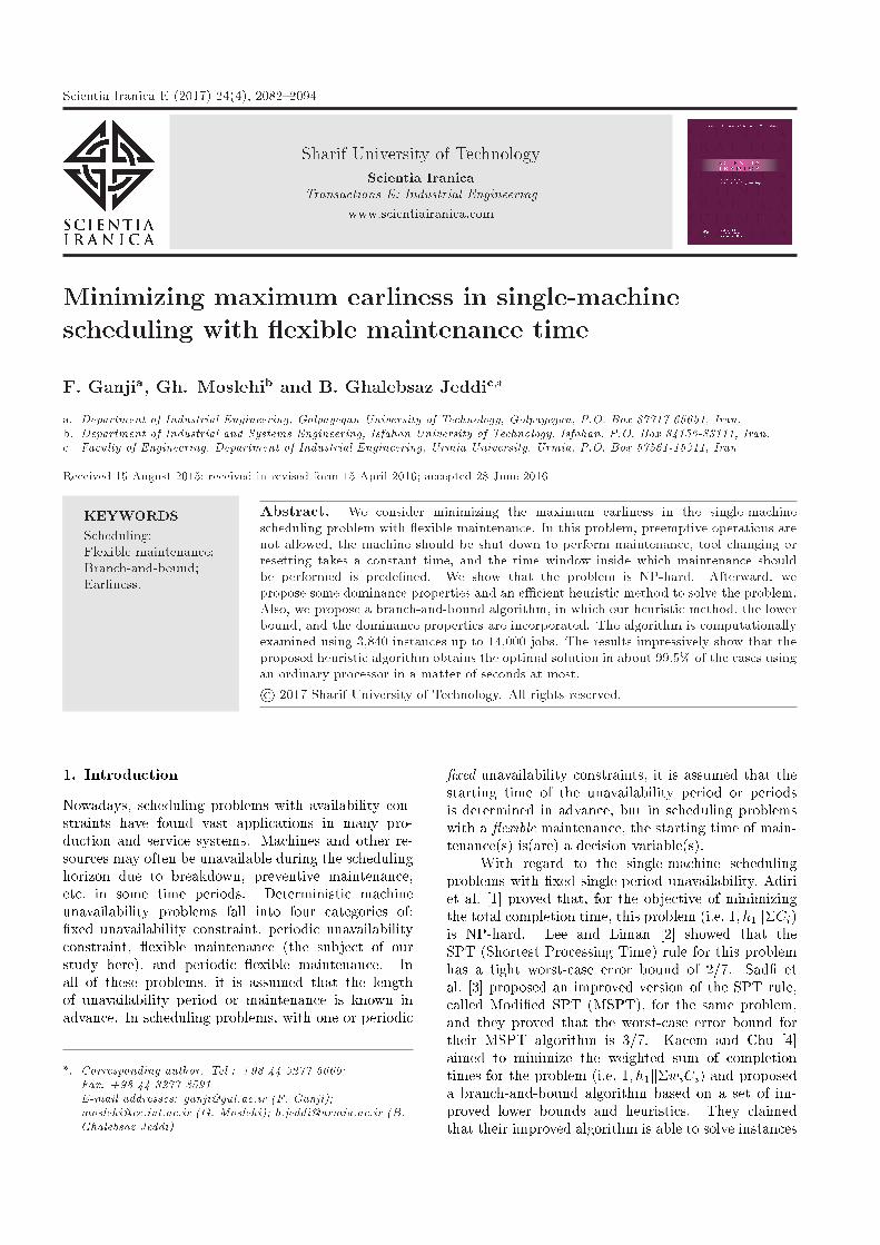
Figure 1. Notional form of the problem at hand.
C(�) Completion time of any set of jobs, e.g.�before or �after
� Immediate (and the only) idle timebefore the maintenance
Ei(�) Earliness of job i in any sequence
Figure 1 depicts the notations of problem 1; h1jfajEmax.
The decision variables are the sequence of thejobs, which also de�nes the starting time of any joband starting time of the maintenance operation.
Major assumptions of the study are as follows:All jobs are of single operation, and preemption or jobsplitting is not allowed (i.e. jobs are nonpreemptive),and they are simultaneously available at the beginningof the planning horizon; all data are integer includingthe processing times; unforced idle time is prohibitedat any point including before the maintenance (i.e.,it is not allowed to create an idle time that can becompletely or partially occupied by a job; in otherwords, � < minfpiji 2 �afterg); the period [u; v], inwhich the maintenance should be performed, has beenarranged in advance and clearly maintenance time, w,is smaller than v � u.
It is important to note that if an unforced idletime was allowed, all jobs could be processed afterthe maximum due date with an arbitrary arrangementso that the maximum earliness becomes zero althoughother criteria, which we do not consider here, may behurt. However, it is not rational to create such idlenessdue to the highly valuable machine time.
Furthermore, in the problem at hand, all jobscannot be processed before the maintenance (i.e.,�pi > v � w); otherwise, the problem reduces tothe case of scheduling without maintenance, where theMinimum Slack Time (MST) sequence is the optimalsolution as d[1] � p[1] � d[2] � p[2] � � � � � d[n] � p[n],where brackets indicate the rankings of the jobs in thesequence [22]. The problem 1; h1jfajEmax has not beenaddressed in the literature. It is suitable to comment onthe complexity of the problem at this point. Molaee [6]showed that the single-machine scheduling problemwith a �xed unavailability constraint (1; h1kEmax)along with the assumption of allowed idle time isNP-hard. Thereby, in a particular situation whenw = v � u, the problem 1; h1jfajEmax converts to1; h1kEmax, so the complexity of 1; h1jfajEmax is at
F. Ganji et al./Scientia Iranica, Transactions E: Industrial Engineering 24 (2017) 2082{2094 2085
least as much as the complexity of 1; h1kEmax, so theproblem at hand is NP-hard.
In this section, we present a few theorems andlemmas to establish two-solution procedures for theproblem. Before discussing the theorems, note thatthe starting time of jobs in �after is not �xed sincewe do not yet know when the maintenance will startand end; however, we will show that the MST ruleis the basis (with some modi�cation) for providing itsoptimal sequence. Also, note that the starting time ofmaintenance in this problem is a decision variable sothat we cannot assume, by default, that maintenanceservice starts at �rst or ends at the last position of themaintenance time window (in that case, 1; h1jfajEmaxconverts to 1; h1kEmax).
Lemma 1: In problem 1; h1jfajEmax, there is anoptimal sequence where jobs in �before and jobs in �afterare ordered according to MST rule.
Proof: We know that the MST rule is the optimalsolution to 1kEmax problem [22]. Jobs are dividedinto groups of `before' and `after' maintenance in thisproblem, where one of them starts processing at timezero (the beginning of the planning horizon) and theother starts right after maintenance. Therefore, eachof them shall be ordered with respect to MST rule. �
Based on this lemma, we introduce some methodshere to solve 1; h1jfajEmax problem. The MST se-quence may generate a feasible sequence for 1; h1kEmaxand 1; h1jfajEmax problems; however, care should betaken because it is not necessarily optimal.
Dominance property 1: Sequences, in which thestarting time of a job in �before is not in [u; v�w], area dominant set for 1; h1jfajEmax problem.
Proof: Denote the last job in �before by job i, andif its starting time is in period [u; v � w] (and conse-quently, it is completed before v�w), then by changingthe position of job i and maintenance activity, thecompletion time of job i increases; therefore, objectivefunction, Emax, will not get worse. �
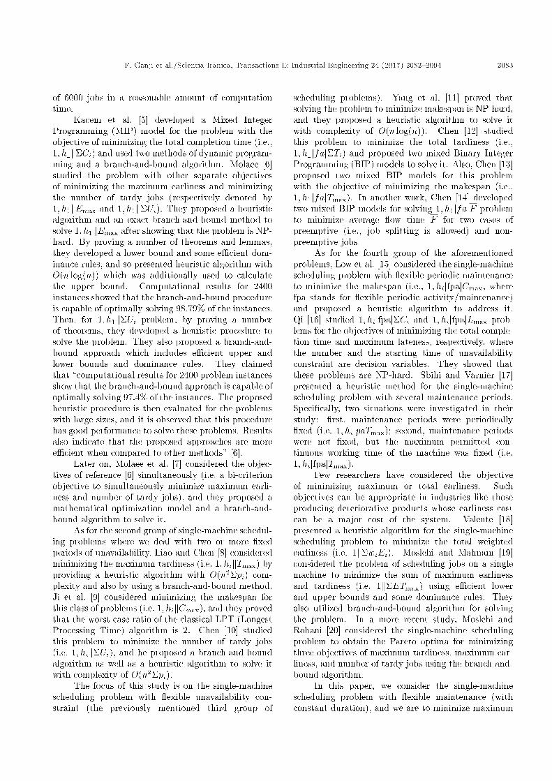
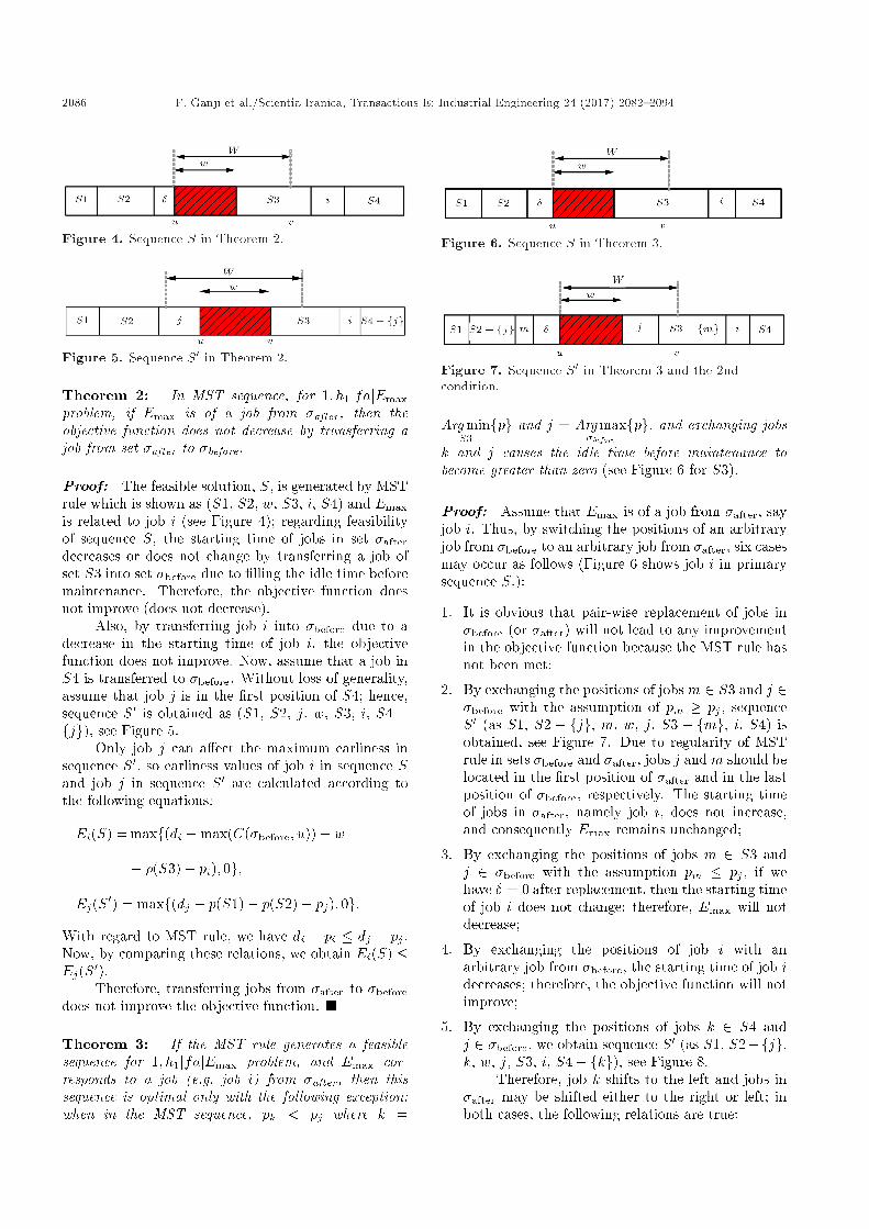
Theorem 1: In the problem 1; h1jfajEmax, MSTsequence is optimal if it generates a feasible solution,no matter where the maintenance is located in [u; v]window, and Emax is of a job from �before.
Proof: Denote a feasible solution, S, obtained byMST rule as (S1, i, S2, w, S3, S4) where Emax is of jobi and Sj is a partial sequence of S, see Figure 2. Weshall now show that no replacement decreases Emax.
By exchanging the positions of an arbitrary jobfrom S1 with an arbitrary job from �after due to the
Figure 2. Sequence S in Theorem 1.
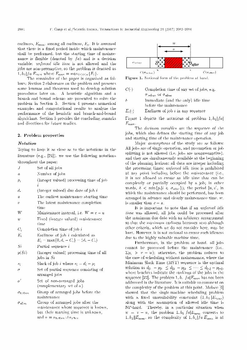
Figure 3. Sequence S0 in Theorem 1.
regularity of MST rule in both �before and �after , thereplaced jobs are set in the �rst position of �after andin the last position of �before, respectively. Thereby,the jobs in set �before located after the replaced job insequence S are shifted to the left and their startingtime decreases; therefore, Emax will not improve.Additionally, by changing the position of a job from S2and an arbitrary job from �after, Emax will not increasebecause the starting time of job i has not changed. Byexchanging job i with an arbitrary job k from �after,sequence S0 as (S1, S2, k, w, i, S3, S4 � fkg) isobtained, see Figure 3. Without loss of generality, itis assumed that job k is located at the �rst positionof S4; two situations may occur: the partial sequence,S2, is not empty, or it is empty.
Assume that partial sequence, S2, is not emptyand job j is the �rst one in S2. Then, the earlinessvalues of jobs i, j, and k in two sequences, S and S0,after switching jobs k and i are as follows:
Ei(S) = maxf(di � p(S1)� pi); 0g;Ek(S0) = maxf(dk � p(S1)� p(S2)� pk); 0g;
and:
Ej(S0) = maxf(dj � p(S1)� pj); 0g;where, by MST rule, we have di�pi � dj�pj . Thus, bycomparing these relations, we conclude that Ei(S) �Ej(S0).
Now, assume that partial sequence, S2, is empty,so job i is located in the last position of sequence S;thereby, regarding MST rule, we have di�pi � dk�pk.By comparing the above relations, we arrive at Ei(S) �Ek(S0).
So, the maximum earliness of sequence S is notalways greater than this value in sequence S0, thenby switching jobs i and k in sequence S, maximumearliness will not diminish. �
Considering the possibility of shifting mainte-nance service back or forth in time, it might be possibleto transfer a job from �after to �before.
2086 F. Ganji et al./Scientia Iranica, Transactions E: Industrial Engineering 24 (2017) 2082{2094
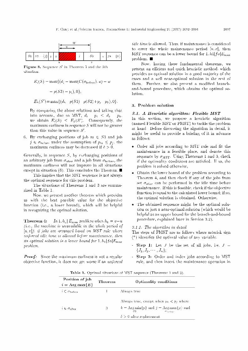
Figure 4. Sequence S in Theorem 2.
Figure 5. Sequence S0 in Theorem 2.
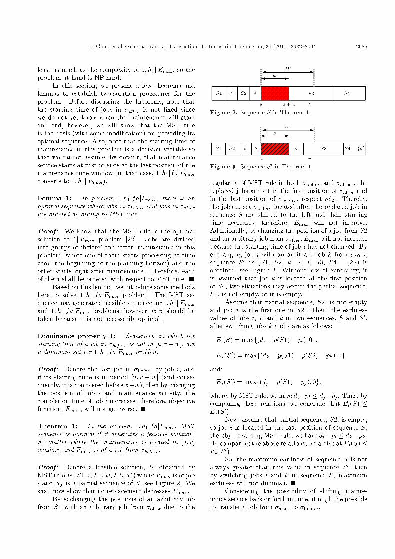
Theorem 2: In MST sequence, for 1; h1jfajEmaxproblem, if Emax is of a job from �after, then theobjective function does not decrease by transferring ajob from set �after to �before.
Proof: The feasible solution, S, is generated by MSTrule which is shown as (S1, S2, w, S3, i, S4) and Emaxis related to job i (see Figure 4); regarding feasibilityof sequence S, the starting time of jobs in set �afterdecreases or does not change by transferring a job ofset S3 into set �before due to �lling the idle time beforemaintenance. Therefore, the objective function doesnot improve (does not decrease).
Also, by transferring job i into �before due to adecrease in the starting time of job i, the objectivefunction does not improve. Now, assume that a job inS4 is transferred to �before. Without loss of generality,assume that job j is in the �rst position of S4; hence,sequence S0 is obtained as (S1, S2, j, w, S3, i, S4 �fjg), see Figure 5.
Only job j can a�ect the maximum earliness insequence S0, so earliness values of job i in sequence Sand job j in sequence S0 are calculated according tothe following equations:
Ei(S) = maxf(di �max(C(�before; u))� w� p(S3)� pi); 0g;
Ej(S0) = maxf(dj � p(S1)� p(S2)� pj); 0g:With regard to MST rule, we have di � pi � dj � pj .Now, by comparing these relations, we obtain Ei(S) �Ej(S0).
Therefore, transferring jobs from �after to �beforedoes not improve the objective function. �
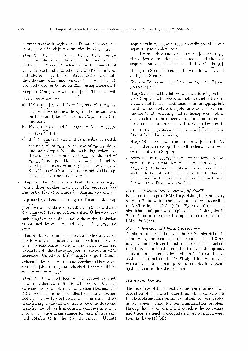
Theorem 3: If the MST rule generates a feasiblesequence for 1; h1jfajEmax problem, and Emax cor-responds to a job (e.g. job i) from �after, then thissequence is optimal only with the following exception:when in the MST sequence, pk < pj where k =
Figure 6. Sequence S in Theorem 3.
Figure 7. Sequence S0 in Theorem 3 and the 2ndcondition.
Arg minS3
fpg and j = Arg max�before
fpg, and exchanging jobs
k and j causes the idle time before maintenance tobecome greater than zero (see Figure 6 for S3).
Proof: Assume that Emax is of a job from �after, sayjob i. Thus, by switching the positions of an arbitraryjob from �before to an arbitrary job from �after, six casesmay occur as follows (Figure 6 shows job i in primarysequence S.):
1. It is obvious that pair-wise replacement of jobs in�before (or �after) will not lead to any improvementin the objective function because the MST rule hasnot been met;
2. By exchanging the positions of jobs m 2 S3 and j 2�before with the assumption of pm � pj , sequenceS0 (as S1, S2 � fjg, m, w, j, S3 � fmg, i, S4) isobtained, see Figure 7. Due to regularity of MSTrule in sets �before and �after, jobs j and m should belocated in the �rst position of �after and in the lastposition of �before, respectively. The starting timeof jobs in �after, namely job i, does not increase,and consequently Emax remains unchanged;
3. By exchanging the positions of jobs m 2 S3 andj 2 �before with the assumption pm � pj , if wehave � = 0 after replacement, then the starting timeof job i does not change; therefore, Emax will notdecrease;
4. By exchanging the positions of job i with anarbitrary job from �before, the starting time of job idecreases; therefore, the objective function will notimprove;
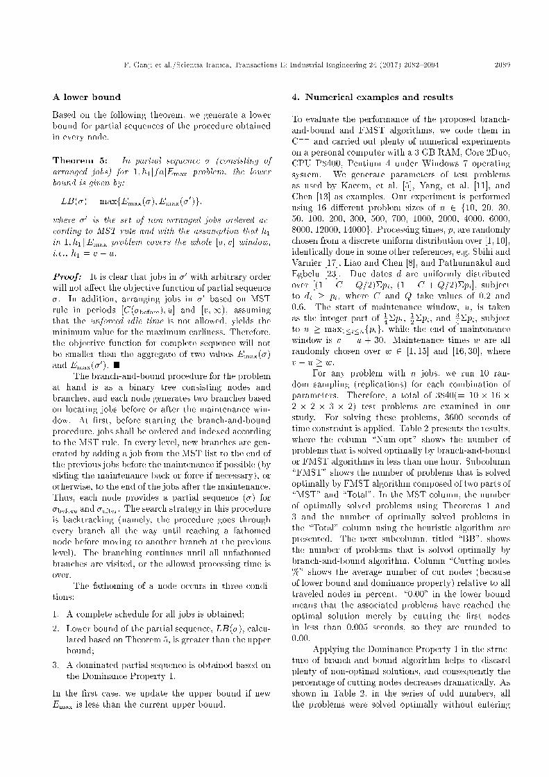
5. By exchanging the positions of jobs k 2 S4 andj 2 �before, we obtain sequence S0 (as S1, S2�fjg,k, w, j, S3, i, S4� fkg), see Figure 8.
Therefore, job k shifts to the left and jobs in�after may be shifted either to the right or left; inboth cases, the following relations are true:
F. Ganji et al./Scientia Iranica, Transactions E: Industrial Engineering 24 (2017) 2082{2094 2087
Figure 8. Sequence S0 in Theorem 3 and the 5thsituation.
Ei(S) = maxf(di �max(C(�before); u)� w� p(S3)� pi); 0g;
Ek(S0)=maxf(dk�p(S1)�p(S2)+pj�pk); 0g:By comparing the above relations and taking thatinto account, due to MST, di � pi � dk � pk,we obtain Ei(S) � Ek(S0). Consequently, themaximum earliness in sequence S will not be greaterthan this value in sequence S0.
6. By exchanging positions of job m 2 S3 and jobj 2 �before under the assumption of pm � pj , themaximum earliness may be decreased if � > 0.
Generally, in sequence S, by exchanging positions ofan arbitrary job from �after and a job from �before, themaximum earliness will not improve in all situationsexcept in situation (6). This concludes the Theorem. �
This implies that the MST sequence is not alwaysthe optimal sequence for this problem.
The situations of Theorems 1 and 3 are summa-rized in Table 1.
Now, we present another theorem which providesus with the best possible value for the objectivefunction (i.e., a lower bound), which will be helpfulin recognizing the optimal solution.
Theorem 4: In 1; h1kEmax problem when h1 = v�u(i.e., the machine is unavailable in the whole period of[u; v]), if jobs are arranged based on MST rule whereunforced idle time is allowed before maintenance, thenits optimal solution is a lower bound for 1; h1jfajEmaxproblem.
Proof: Since the maximum earliness is not a regularobjective function, it does not get worse if an unforced
idle time is allowed. Thus, if maintenance is consideredto cover the whole maintenance period [u; v], thenMST sequence can be a lower bound for 1; h1jfajEmaxproblem. �
Now, having these fundamental theorems, wepresent an e�cient and quick heuristic method, whichprovides an optimal solution in a good majority of thecases and a well near-optimal solution in the rest ofthem. Further, we also present a modi�ed branch-and-bound procedure, which obtains the optimal so-lution.
3. Problem solution
3.1. A Heuristic algorithm: Flexible MSTIn this section, we propose a heuristic algorithm(named Flexible MST or FMST) to tackle the problemat hand. Before discussing the algorithm in detail, itmight be useful to provide a brie�ng of it in advanceas follows:
� Order all jobs according to MST rule and �t themaintenance in a feasible place, and denote thissequence by �MST. Using Theorems 1 and 3, checkif the optimality conditions are satis�ed. If so, theproblem is solved otherwise,
� Obtain the lower bound of the problem according toTheorem 4, and then check if any of the jobs fromset �after can be performed in the idle time beforemaintenance. If this is feasible, check if the objectivefunction is equal to the calculated lower bound; if so,the optimal solution is obtained. Otherwise,
� The obtained sequence might be the optimal solu-tion or just a near-optimal solution (which would behelpful as an upper bound for the branch-and-boundprocedure, explained later in Section 3.2).
3.1.1. The algorithm in detailThe steps of FMST are as follows where asterisk sign(*) identi�es the optimal value of any variable.
- Step 1: Let J be the set of all jobs, i.e. J =fJ1; J2; � � � ; Jng;
- Step 2: Order and index jobs according to MSTrule, and then insert the maintenance operation in
Table 1. Optimal situations of MST sequence (Theorems 1 and 3).
Position of jobi = Arg maxfEg Theorem Optimality conditions
i 2 �before 1 Always true
i 2 �after 3
Always true, except when pk < pj where
k = Arg minS3
fpg and j = Arg max�before
fpg and
� > 0 after replacement
2088 F. Ganji et al./Scientia Iranica, Transactions E: Industrial Engineering 24 (2017) 2082{2094
between so that it begins at u. Denote this sequenceby �MST and its objective function by Emax�MST;
- Step 3: Set �1 = �MST. Let m be a counterfor the number of scheduled jobs after maintenanceand m = 1; 2; � � � ;M , where M is the size of set�after, created �rstly based on the MST schedule; so,initially, m = 1. Let i = Arg maxfEg. Calculatethe idle time before maintenance � = u�C(�before).Calculate a lower bound for Emax using Theorem 4;
- Step 4: Compare � with min�afterfpig. Then, we will
face three situations:a) If � < min
�afterfpig and if i = Arg maxfEg 2 �before,
then we have obtained the optimal solution basedon Theorem 1; let �� = �1 and E�max = Emax(�1)and exit;
b) If � < min�afterfpig and i = Arg maxfEg 2 �after, go
to Step 5. But;c) if � > min
�afterfpig and if it is possible to switch
the �rst job of �after to the end of �before, do soand start Step 4 from the beginning; otherwise,if switching the �rst job of �after to the end of�before is not possible, let m = m + 1 and goto Step 6, unless m = M ; in that case, go toStep 11 to exit (Note that at the end of this step,a feasible sequence is obtained.);
- Step 5: Let S3 be a subset of jobs in �afterwith indices smaller than i in MST sequence (seeFigure 6). If pk < pj where k = Arg min
S3fpg and j =
Arg max�before
fpg, then, according to Theorem 3, swap
jobs j with k, update �1 and Emax(�1), check if new� � min
�afterfpig, then go to Step 7 if so. Otherwise, the
switching is not possible, and so the optimal solutionis obtained; let �� = �1 and E�max = Emax(�1) andexit;
- Step 6: By starting from job m and checking everyjob forward, if transferring any job from �after to�before is possible, add that job into �before accordingto MST; note that the other jobs are already in MSTsequence. Update �. If � � min
�afterfpig, go to Step7;
otherwise let m = m + 1 and continue this processuntil all jobs in �after are checked if they could betransferred to �before;
- Step 7: If Emax(�) does not correspond to a jobin �before, then go to Step 8. Otherwise, if Emax(�)corresponds to a job in �before, then (because theMST sequence is now shu�ed) do the following:Let m = m + 1, start from job m in �after, if itstransferring to the end of �before is possible, do so andtransfer the job with maximum earliness in �beforeinto �after, slide maintenance forward if necessaryand possible to �t the job into �before. Update
sequences in �before and �after according to MST ruleseparately and calculate �.
By selecting and replacing all jobs in �after,the objective function is calculated, and the bestsequence among them is selected. If � � min
�afterfpig,
then go to Step 11 to exit; otherwise, let m = m+ 1and go to Step 9;
- Step 8: Let m = i + 1 where i = Arg maxfEg andgo to Step 9;
- Step 9: If switching job m to �before is not possible,go to Step 10. Otherwise, add job m (a job after i) to�before, and then let maintenance in an appropriateposition and update the jobs in �before, �after andupdate �. By selecting and replacing every job in�after, calculate the objective function and select thebest sequence among them. If � � min
�afterfpig, go to
Step 11 to exit; otherwise, let m = m+ 1 and repeatStep 9 from the beginning;
- Step 10: If m = M , the number of jobs in initial�after, then go to Step 11 to exit; otherwise, let m =m+ 1 and go to Step 9;
- Step 11: If Emax(�1) is equal to the lower bound,then �1 is optimal, let �� = �1 and E�max =Emax(�1). Otherwise, a solution is obtained whichstill might be optimal or just near optimal (This willbe checked by the branch-and-bound algorithm inSection 3.2.). Exit the algorithm.
3.1.2. Computational complexity of FMSTBased on the steps of FMST algorithm, its complexityat Step 2, in which the jobs are ordered accordingto MST rule, is O(n log(n)). By proceeding in thealgorithm and pair-wise replacement of the jobs inSteps 7 and 9, the overall complexity of the proposedFMST is O(n2).
3.2. A branch-and-bound procedureAs shown in the �nal step of the FMST algorithm, insome cases, the conditions of Theorems 1 and 3 arenot met nor the lower bound of Theorem 4 is reached;therefore, the algorithm could not obtain the optimalsolution. In such cases, by having a feasible and near-optimal solution from the FMST algorithm, we proceedwith a branch-and-bound procedure to obtain an exactoptimal solution for the problem.
An upper bound
The quantity of the objective function returned fromexecution of the FMST algorithm, which correspondsto a feasible and near-optimal solution, can be regardedas an upper bound for our minimization problem.Having this upper bound will expedite the procedure,and there is a need to calculate a lower bound in everystep, as discussed below.
F. Ganji et al./Scientia Iranica, Transactions E: Industrial Engineering 24 (2017) 2082{2094 2089
A lower bound
Based on the following theorem, we generate a lowerbound for partial sequences of the procedure obtainedin every node.
Theorem 5: In partial sequence � (consisting ofarranged jobs) for 1; h1jfajEmax problem, the lowerbound is given by:
LB(�) = maxfEmax(�); Emax(�0)g;where �0 is the set of non-arranged jobs ordered ac-cording to MST rule and with the assumption that h1in 1; h1kEmax problem covers the whole [u; v] window,i.e., h1 = v � u.
Proof: It is clear that jobs in �0 with arbitrary orderwill not a�ect the objective function of partial sequence�. In addition, arranging jobs in �0 based on MSTrule in periods [C(�before); u] and [v;1), assumingthat the unforced idle time is not allowed, yields theminimum value for the maximum earliness. Therefore,the objective function for complete sequence will notbe smaller than the aggregate of two values Emax(�)and Emax(�0). �
The branch-and-bound procedure for the problemat hand is as a binary tree consisting nodes andbranches, and each node generates two branches basedon locating jobs before or after the maintenance win-dow. At �rst, before starting the branch-and-boundprocedure, jobs shall be ordered and indexed accordingto the MST rule. In every level, new branches are gen-erated by adding a job from the MST list to the end ofthe previous jobs before the maintenance if possible (bysliding the maintenance back or force if necessary), orotherwise, to the end of the jobs after the maintenance.Thus, each node provides a partial sequence (�) for�before and �after. The search strategy in this procedureis backtracking (namely, the procedure goes throughevery branch all the way until reaching a fathomednode before moving to another branch at the previouslevel). The branching continues until all unfathomedbranches are visited, or the allowed processing time isover.
The fathoming of a node occurs in three condi-tions:
1. A complete schedule for all jobs is obtained;2. Lower bound of the partial sequence, LB(�), calcu-
lated based on Theorem 5, is greater than the upperbound;
3. A dominated partial sequence is obtained based onthe Dominance Property 1.
In the �rst case, we update the upper bound if newEmax is less than the current upper bound.
4. Numerical examples and results
To evaluate the performance of the proposed branch-and-bound and FMST algorithms, we code them inC++ and carried out plenty of numerical experimentson a personal computer with a 3 GB RAM, Core 2Duo,CPU P8400, Pentium 4 under Windows 7 operatingsystem. We generate parameters of test problemsas used by Kacem, et al. [5], Yang, et al. [11], andChen [13] as examples. Our experiment is performedusing 16 di�erent problem sizes of n 2 f10, 20, 30,50, 100, 200, 300, 500, 700, 1000, 2000, 4000, 6000,8000, 12000, 14000g. Processing times, p, are randomlychosen from a discrete uniform distribution over [1; 10],identically done in some other references, e.g. Sbihi andVarnier [17], Liao and Chen [8], and Pathumnakul andEgbelu [23]. Due dates d are uniformly distributedover [(1 � C � Q=2)�pi, (1 � C + Q=2)�pi], subjectto di � pi, where C and Q take values of 0.2 and0.6. The start of maintenance window, u, is takenas the integer part of 1
4�pi, 12�pi, and 3
4�pi, subjectto u � max1�i�nfpig, while the end of maintenancewindow is v = u + 30. Maintenance times w are allrandomly chosen over w 2 [1; 15] and [16; 30], wherev � u � w.
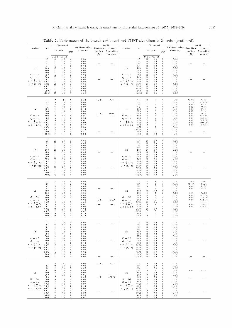
For any problem with n jobs, we run 10 ran-dom sampling (replications) for each combination ofparameters. Therefore, a total of 3840(= 10 � 16 �2 � 2 � 3 � 2) test problems are examined in ourstudy. For solving these problems, 3600 seconds oftime constraint is applied. Table 2 presents the results,where the column \Num-opt" shows the number ofproblems that is solved optimally by branch-and-boundor FMST algorithms in less than one hour. Subcolumn\FMST" shows the number of problems that is solvedoptimally by FMST algorithm composed of two parts of\MST" and \Total". In the MST column, the numberof optimally solved problems using Theorems 1 and3 and the number of optimally solved problems inthe \Total" column using the heuristic algorithm arepresented. The next subcolumn, titled \BB", showsthe number of problems that is solved optimally bybranch-and-bound algorithm. Column \Cutting nodes%" shows the average number of cut nodes (becauseof lower bound and dominance property) relative to alltraveled nodes in percent. \0.00" in the lower boundmeans that the associated problems have reached theoptimal solution merely by cutting the �rst nodesin less than 0.005 seconds, so they are rounded to0.00.
Applying the Dominance Property 1 in the struc-ture of branch-and-bound algorithm helps to discardplenty of non-optimal solutions, and consequently thepercentage of cutting nodes decreases dramatically. Asshown in Table 2, in the series of odd numbers, allthe problems were solved optimally without entering
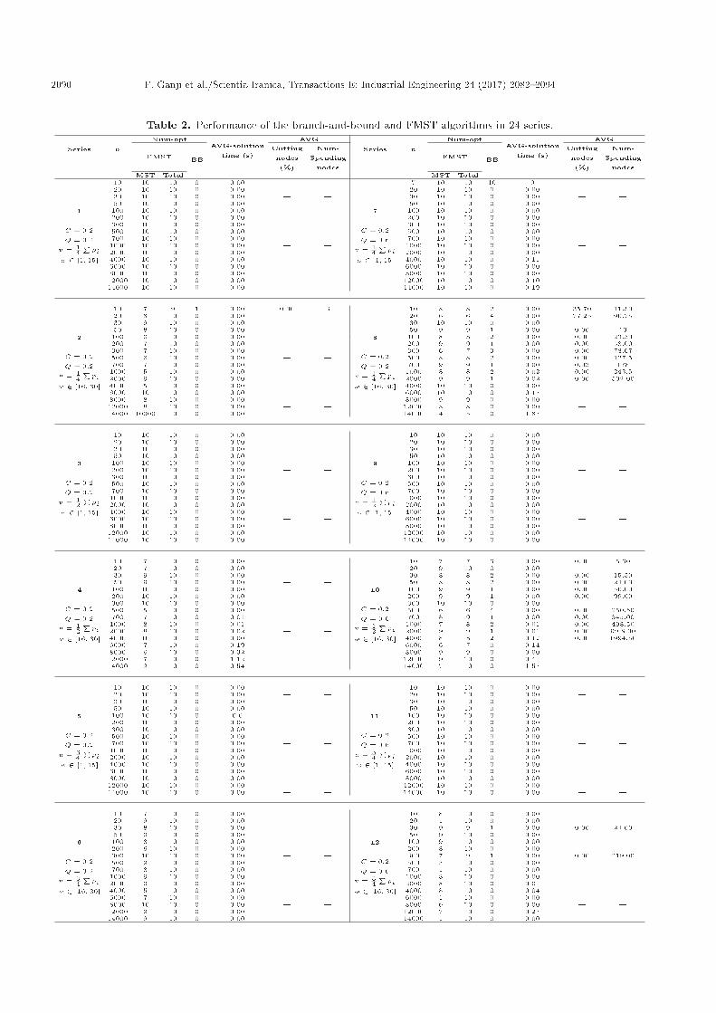
2090 F. Ganji et al./Scientia Iranica, Transactions E: Industrial Engineering 24 (2017) 2082{2094
Table 2. Performance of the branch-and-bound and FMST algorithms in 24 series.
Series n
Num-optAVG-solution
time (s)
AVG
Series n
Num-optAVG-solution
time (s)
AVG
FMST BB
Cuttingnodes(%)
Num-Spending
nodes
FMST BB
Cuttingnodes(%)
Num-Spending
nodesMST Total MST Total
1
C = 0:2Q = 0:2
u = 14Ppi
w 2 [1; 15]
10 10 10 0 0.00 | |
7
C = 0:2Q = 0:6
u = 14Ppi
w 2 [1; 15]
7 10 10 10 0 | |20 10 10 0 0.00 | | 20 10 10 0 0.00 | |30 10 10 0 0.00 | | 30 10 10 0 0.00 | |50 10 10 0 0.00 | | 50 10 10 0 0.00 | |100 10 10 0 0.00 | | 100 10 10 0 0.00 | |200 10 10 0 0.00 | | 200 10 10 0 0.00 | |300 10 10 0 0.00 | | 300 10 10 0 0.00 | |500 10 10 0 0.00 | | 500 10 10 0 0.00 | |700 10 10 0 0.00 | | 700 10 10 0 0.00 | |1000 10 10 0 0.00 | | 1000 10 10 0 0.00 | |2000 10 10 0 0.00 | | 2000 10 10 0 0.00 | |4000 10 10 0 0.00 | | 4000 10 10 0 0.11 | |6000 10 10 0 0.00 | | 6000 10 10 0 0.00 | |8000 10 10 0 0.00 | | 8000 10 10 0 0.00 | |12000 10 10 0 0.00 | | 12000 10 10 0 0.10 | {14000 10 10 0 0.00 | | 14000 10 10 0 0.19 | {
2
C = 0:2Q = 0:2
u = 14Ppi
w 2 [16; 30]
10 7 9 1 0.00 0.00 3
8
C = 0:2Q = 0:2
u = 14Ppi
w 2 [16; 30]
10 8 8 2 0.00 35.70 11.5020 8 10 0 0.00 | | 20 6 6 4 0.00 77.25 90.7530 9 10 0 0.00 | | 30 10 10 0 0.00 | |50 8 10 0 0.00 | | 50 9 9 1 0.00 0.00 13100 6 10 0 0.00 | | 100 8 8 2 0.00 0.00 23.50200 7 10 0 0.00 | | 200 9 9 1 0.00 0.00 58.00300 7 10 0 0.00 | | 300 6 7 3 0.00 0.00 78.67500 6 10 0 0.00 | | 500 8 8 2 0.00 0.00 127.5700 7 10 0 0.00 | | 700 9 9 1 0.00 0.03 1781000 5 10 0 0.00 | | 1000 8 8 2 0.02 0.00 243.52000 9 10 0 0.00 | | 2000 9 9 1 0.02 0.00 502.004000 5 10 0 0.00 | | 4000 10 10 0 0.00 | |6000 10 10 0 0.00 | | 6000 10 10 0 0.17 | |8000 8 10 0 0.00 | | 8000 9 9 0 0.00 | |12000 8 10 0 0.00 | | 12000 8 8 0 0.00 | |14000 10000 10 0 0.00 | | 14000 4 5 0 1.87 | |
3
C = 0:2Q = 0:2
u = 12Ppi
w 2 [1; 15]
10 10 10 0 0.00 | |
9
C = 0:2Q = 0:6
u = 12Ppi
w 2 [1; 15]
10 10 10 0 0.00 | |20 10 10 0 0.00 | | 20 10 10 0 0.00 | |30 10 10 0 0.00 | | 30 10 10 0 0.00 | |50 10 10 0 0.00 | | 50 10 10 0 0.00 | |100 10 10 0 0.00 | | 100 10 10 0 0.00 | |200 10 10 0 0.00 | | 200 10 10 0 0.00 | |300 10 10 0 0.00 | | 300 10 10 0 0.00 | |500 10 10 0 0.00 | | 500 10 10 0 0.00 | |700 10 10 0 0.00 | | 700 10 10 0 0.00 | |1000 10 10 0 0.00 | | 1000 10 10 0 0.00 | |2000 10 10 0 0.00 | | 2000 10 10 0 0.00 | |4000 10 10 0 0.00 | | 4000 10 10 0 0.00 | |6000 10 10 0 0.00 | | 6000 10 10 0 0.00 | |8000 10 10 0 0.00 | | 8000 10 10 0 0.00 | |12000 10 10 0 0.00 | | 12000 10 10 0 0.00 | |14000 10 10 0 0.00 | | 14000 10 10 0 0.00 | |
4
C = 0:2Q = 0:2
u = 12Ppi
w 2 [16; 30]
10 7 10 0 0.00 | |
10
C = 0:2Q = 0:6
u = 12Ppi
w 2 [16; 30]
10 7 7 3 0.00 0.00 5.3020 7 10 0 0.00 | | 20 9 10 0 0.00 | |30 9 10 0 0.00 | | 30 8 8 2 0.00 0.00 15.5050 9 10 0 0.00 | | 50 8 8 2 0.00 0.00 24.00100 10 10 0 0.00 | | 100 9 9 1 0.00 0.00 50.00200 10 10 0 0.00 | | 200 9 9 1 0.00 0.00 99.00300 10 10 0 0.00 | | 300 10 10 0 0.00 | |500 5 10 0 0.00 | | 500 6 6 4 0.00 0.00 250.50700 7 10 0 0.01 | | 700 8 9 1 0.00 0.00 345.001000 8 10 0 0.01 | | 1000 7 8 2 0.01 0.00 498.502000 8 10 0 0.02 | | 2000 9 9 1 0.01 0.00 99.8.004000 10 10 0 0.00 | | 4000 8 8 2 0.12 0.00 1994.506000 7 10 0 0.19 | | 6000 6 7 0 0.14 | |8000 6 10 0 0.32 | | 8000 9 9 0 0.00 | |12000 7 10 0 1.12 | | 12000 9 10 0 0.41 | |14000 9 10 0 0.54 | | 14000 7 10 0 1.57 | |
5
C = 0:2Q = 0:2
u = 34Ppi
w 2 [1; 15]
10 10 10 0 0.00 | |
11
C = 0:2Q = 0:6
u = 34Ppi
w 2 [1; 15]
10 10 10 0 0.00 | |20 10 10 0 0.00 | | 20 10 10 0 0.00 | |30 10 10 0 0.00 | | 30 10 10 0 0.00 | |50 10 10 0 0.00 | | 50 10 10 0 0.00 | |100 10 10 0 0.0 | | 100 10 10 0 0.00 | |200 10 10 0 0.00 | | 200 10 10 0 0.00 | |300 10 10 0 0.00 | | 300 10 10 0 0.00 | |500 10 10 0 0.00 | | 500 10 10 0 0.00 | |700 10 10 0 0.00 | | 700 10 10 0 0.00 | |1000 10 10 0 0.00 | | 1000 10 10 0 0.00 | |2000 10 10 0 0.00 | | 2000 10 10 0 0.00 | |4000 10 10 0 0.00 | | 4000 10 10 0 0.00 | |6000 10 10 0 0.00 | | 6000 10 10 0 0.00 | |8000 10 10 0 0.00 | | 8000 10 10 0 0.00 | |12000 10 10 0 0.00 | | 12000 10 10 0 0.00 | |14000 10 10 0 0.00 | | 14000 10 10 0 0.00 | |
6
C = 0:2Q = 0:2
u = 34Ppi
w 2 [16; 30]
10 7 10 0 0.00 | |
12
C = 0:2Q = 0:6
u = 34Ppi
w 2 [16; 30]
10 8 10 0 0.00 | |20 9 10 0 0.00 | | 20 1 10 0 0.00 | |30 8 10 0 0.00 | | 30 9 9 1 0.00 0.00 24.0050 9 10 0 0.00 | | 50 9 10 0 0.00 | |100 8 10 0 0.00 | | 100 9 10 0 0.00 | |200 6 10 0 0.00 | | 200 8 10 0 0.00 | |300 10 10 0 0.00 | | 300 7 9 1 0.00 0.00 219.00500 9 10 0 0.00 | | 500 5 10 0 0.00 | |700 8 10 0 0.00 | | 700 1 10 0 0.00 | |1000 9 10 0 0.00 | | 1000 8 10 0 0.00 | |2000 9 10 0 0.00 | | 2000 8 10 0 0.01 | |4000 5 10 0 0.00 | | 4000 8 10 0 0.04 | |6000 7 10 0 0.00 | | 6000 1 10 0 0.00 | |8000 10 10 0 0.00 | | 8000 6 10 0 0.00 | |12000 9 10 0 0.00 | | 12000 7 10 0 0.27 | |14000 9 10 0 0.00 | | 14000 1 10 0 0.00 | |
F. Ganji et al./Scientia Iranica, Transactions E: Industrial Engineering 24 (2017) 2082{2094 2091
Table 2. Performance of the branch-and-bound and FMST algorithms in 24 series (continued).
Series n
Num-optAVG-solution
time (s)
AVG
Series n
Num-optAVG-solution
time (s)
AVG
FMST BB
Cuttingnodes(%)
Num-Spending
nodes
FMST BB
Cuttingnodes(%)
Num-Spending
nodesMST Total MST Total
13
C = 0:6Q = 0:2
u = 14Ppi
w 2 [1; 15]
10 10 10 0 0.00 | |
19
C = 0:6Q = 0:6
u = 14Ppi
w 2 [1; 15]
10 10 10 0 0.00 | |20 10 10 0 0.00 | | 20 10 10 0 0.00 | |30 10 10 0 0.00 | | 30 10 10 0 0.00 | |50 10 10 0 0.00 | | 50 10 10 0 0.00 | |100 10 10 0 0.00 | | 100 10 10 0 0.00 | |200 10 10 0 0.00 | | 200 10 10 0 0.00 | |300 10 10 0 0.00 | | 300 10 10 0 0.00 | |500 10 10 0 0.00 | | 500 10 10 0 0.00 | |700 10 10 0 0.00 | | 700 10 10 0 0.00 | |1000 10 10 0 0.00 | | 1000 10 10 0 0.00 | |2000 10 10 0 0.00 | | 2000 10 10 0 0.00 | |4000 10 10 0 0.00 | | 4000 10 10 0 0.00 | |6000 10 10 0 0.00 | | 6000 10 10 0 0.00 | |8000 10 10 0 0.00 | | 8000 10 10 0 0.00 | |12000 10 10 0 0.00 | | 12000 10 10 0 0.00 | |14000 10 10 0 0.00 | | 14000 10 10 0 0.00 | |
14
C = 0:6Q = 0:2
u = 14Ppi
w 2 [16; 30]
10 7 7 3 0.00 0.00 7.00
20
C = 0:6Q = 0:6
u = 14Ppi
w 2 [16; 30]
10 8 8 2 0.00 52.20 23.0020 9 10 0 0.00 | | 20 7 7 3 0.00 30.10 270.0030 8 10 0 0.00 | | 30 7 7 3 0.00 0.00 26.0050 10 10 0 0.00 | | 50 8 8 2 0.00 0.00 14.00100 10 10 0 0.00 | | 100 9 9 1 0.00 0.00 25.00200 10 10 0 0.00 | | 200 9 9 1 0.00 0.00 67.00300 7 9 1 0.00 0.00 70.00 300 8 8 2 0.00 0.00 78.50500 6 10 0 0.01 | | 500 6 6 4 0.00 0.00 128.75700 8 10 0 0.00 | | 700 9 9 1 0.00 0.00 169.001000 9 10 0 0.01 | | 1000 8 8 2 0.01 0.00 253.002000 8 10 0 0.03 | | 2000 9 9 1 0.02 0.00 501.004000 9 10 0 0.07 | | 4000 9 9 1 0.06 0.00 1005.006000 10 10 0 0.00 | | 6000 9 9 1 0.00 | |8000 4 10 0 1.25 | | 8000 9 9 1 0.00 | |12000 8 10 0 0.87 | | 12000 9 9 1 0.00 | |14000 9 10 0 0.90 | | 14000 10 10 0 0.00 | |
15
C = 0:6Q = 0:2
u = 12Ppi
w 2 [1; 15]
10 10 10 0 0.00 | |
21
C = 0:6Q = 0:6
u = 12Ppi
w 2 [1; 15]
10 10 10 0 0.00 | |20 10 10 0 0.00 | | 20 10 10 0 0.00 | |30 10 10 0 0.00 | | 30 10 10 0 0.00 | |50 10 10 0 0.00 | | 50 10 10 0 0.00 | |100 10 10 0 0.00 | | 100 10 10 0 0.00 | |200 10 10 0 0.00 | | 200 10 10 0 0.00 | |300 10 10 0 0.00 | | 300 10 10 0 0.00 | |500 10 10 0 0.00 | | 500 10 10 0 0.00 | |700 10 10 0 0.00 | | 700 10 10 0 0.00 | |1000 10 10 0 0.00 | | 1000 10 10 0 0.00 | |2000 10 10 0 0.00 | | 2000 10 10 0 0.00 | |4000 10 10 0 0.00 | | 4000 10 10 0 0.00 | |6000 10 10 0 0.00 | | 6000 10 10 0 0.00 | |8000 10 10 0 0.00 | | 8000 10 10 0 0.00 | |12000 10 10 0 0.00 | | 12000 10 10 0 0.00 | |14000 10 10 0 0.00 | | 14000 10 10 0 0.00 | |
16
C = 0:6Q = 0:2
u = 14Ppi
w 2 [16; 30]
10 8 10 0 0.00 | |
22
C = 0:6Q = 0:6
u = 12Ppi
w 2 [16; 30]
10 7 7 3 0.00 12.96 8.0020 7 10 0 0.00 | | 20 9 9 1 0.00 35.40 48.0030 9 10 0 0.00 | | 30 9 9 1 0.00 0.00 14.0050 7 10 0 0.00 | | 50 7 7 3 0.00 0.00 26.00100 9 10 0 0.00 | | 100 10 10 0 0.00 | |200 1 10 0 0.00 | | 200 9 9 1 0.00 0.00 96.00300 9 10 0 0.00 | | 300 8 8 2 0.00 0.00 152.00500 8 10 0 0.00 | | 500 9 9 1 0.00 0.00 250.00700 6 9 1 0.00 0.00 353.00 700 9 9 1 0.00 0.00 351.001000 9 10 0 0.00 | | 1000 10 10 0 0.00 | |2000 9 10 0 0.01 | | 2000 8 8 2 0.03 0.00 1009.504000 7 10 0 0.06 | | 4000 9 9 1 0.05 0.00 2010.006000 9 10 0 0.08 | | 6000 10 10 0 0.00 | |8000 9 10 0 0.08 | | 8000 7 7 0 0.00 | |12000 9 10 0 0.13 { | 12000 7 7 0 0.39 | |14000 9 10 0 0.42 | | 14000 9 9 0 0.55 | |
17
C = 0:6Q = 0:2
u = 34Ppi
w 2 [1; 15]
10 10 10 0 0.00 | |
23
C = 0:6Q = 0:6
u = 12Ppi
w 2 [1; 15]
10 10 10 0 0.00 | |20 10 10 0 0.00 | | 20 10 10 0 0.00 | |30 10 10 0 0.00 | | 30 10 10 0 0.00 | |50 10 10 0 0.00 | | 50 10 10 0 0.00 | |100 10 10 0 0.00 | | 100 10 10 0 0.00 | |200 10 10 0 0.00 | | 200 10 10 0 0.00 | |300 10 10 0 0.00 | | 300 10 10 0 0.00 | |500 10 10 0 0.00 | | 500 10 10 0 0.00 | |700 10 10 0 0.00 | | 700 10 10 0 0.00 | |1000 10 10 0 0.00 | | 1000 10 10 0 0.00 | |2000 10 10 0 0.00 | | 2000 10 10 0 0.00 | |4000 10 10 0 0.00 | | 4000 10 10 0 0.00 | |6000 10 10 0 0.00 | | 6000 10 10 0 0.00 | |8000 10 10 0 0.00 | | 8000 10 10 0 0.00 | |12000 10 10 0 0.00 | | 12000 10 10 0 0.00 | |14000 10 10 0 0.00 | | 14000 10 10 0 0.00 | |
18
C = 0:6Q = 0:2
u = 34Ppi
w 2 [16; 30]
10 8 9 1 0.00 0.00 8.00
24
C = 0:6Q = 0:6
u = 12Ppi
w 2 [1; 15]
10 9 10 0 0.00 | |20 9 10 0 0.00 | | 20 9 10 0 0.00 | |30 9 10 0 0.00 | | 30 1 10 0 0.00 | |50 6 10 0 0.00 | | 50 8 9 1 0.00 0.00 41.00100 8 10 0 0.00 | | 100 1 10 0 0.00 | |200 8 10 0 0.01 | | 200 8 10 0 0.00 | |300 7 9 1 0.00 0.00 224.00 300 5 10 0 0.00 | |500 8 10 0 0.00 | | 500 8 10 0 0.00 | |700 8 10 0 0.00 | | 700 8 10 0 0.00 | |1000 1 10 0 0.00 | | 1000 7 10 0 0.00 | |2000 1 10 0 0.00 | | 2000 1 10 0 0.00 | |4000 8 10 0 0.04 | | 4000 1 10 0 0.00 | |6000 8 10 0 0.10 | | 6000 9 10 0 0.06 | |8000 9 10 0 0.03 | | 8000 9 10 0 0.04 | |12000 9 10 0 0.09 | | 12000 10 10 0 0.00 | |14000 6 10 0 0.67 | | 14000 8 10 0 0.31 | |
2092 F. Ganji et al./Scientia Iranica, Transactions E: Industrial Engineering 24 (2017) 2082{2094
the branch-and-bound algorithm, and also satisfactoryresults were obtained for the rest of the series. Amongthese 24 series, 99.48% (i.e., 3820 out of 3840) of theproblems were solved optimally in a matter of a coupleof seconds at most.
In the series of odd numbers, the ability of FMSTalgorithm to obtain the optimal solution is very high.This might be due to their short-time maintenanceactivity, and consequently high otation in these series.Larger u in even series leads to decreasing the numberof early jobs in �after at the optimal solution, and verylikely, the maximum earliness is obtained from the jobsin �before. Thereby, for large u, it is likely that in MSTsequence, the job with maximum earliness is locatedbefore the maintenance. Thus, due to the large valueof u, the number of problems that is optimal basedon Theorem 1 increases, and also probability of e�ectof switching a job from �after to �before on maximumearliness decreases.
In series 2, 8, 14, and 20 where u possessesthe least value, 81.87% of 640 problems were solvedoptimally by Theorem 1, 10.81% by FMST algorithm,and 7.31% by branch-and-bound algorithm. In theseseries, 1.71% of the problems were left unsolved.It is seen in Figure 9 that the performance of theheuristic algorithm is higher for larger u. So, inseries 6, 12, 18, and 24 where u has the highestvalue, e�ciency of the heuristic algorithm has takenits highest value; in these series, it can solve 99.21%of the problems optimally, and the proportion of thetimes used by the branch-and-bound procedure is0.78%.
From Table 2, we also observe that the solutiontime, among the problems whose optimal solutionswere achieved, has minor changes in terms of u (seethe series 1, 2, 7, 8, 13, 14, 19, 20 for u = 1
4�pi, series3, 4, 9, 10, 15, 16, 21, and 22 for u = 1
2�pi, and series5, 6, 11, 12 17, 18, 23, and 24 for u= 3
4�pi).It is important to further observe how changes in
w a�ect the time until reaching the optimal solution.According to Table 2, in the series of odd numbers,(i.e., 1; 3; � � � ; 23) where w is in [1; 15], all problemswere solved in less than 0.005 seconds on average on
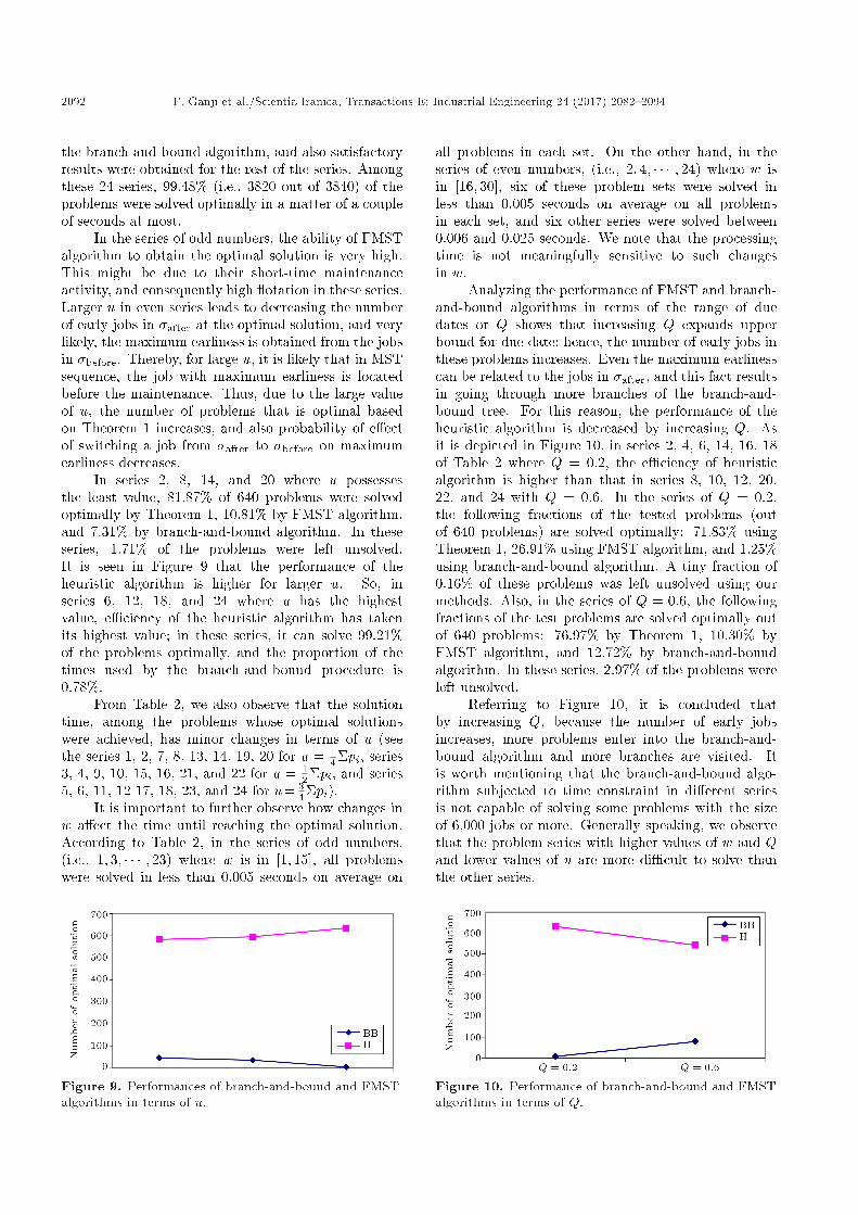
Figure 9. Performances of branch-and-bound and FMSTalgorithms in terms of u.
all problems in each set. On the other hand, in theseries of even numbers, (i.e., 2; 4; � � � ; 24) where w isin [16; 30], six of these problem sets were solved inless than 0.005 seconds on average on all problemsin each set, and six other series were solved between0.006 and 0.025 seconds. We note that the processingtime is not meaningfully sensitive to such changesin w.
Analyzing the performance of FMST and branch-and-bound algorithms in terms of the range of duedates or Q shows that increasing Q expands upperbound for due date; hence, the number of early jobs inthese problems increases. Even the maximum earlinesscan be related to the jobs in �after, and this fact resultsin going through more branches of the branch-and-bound tree. For this reason, the performance of theheuristic algorithm is decreased by increasing Q. Asit is depicted in Figure 10, in series 2, 4, 6, 14, 16, 18of Table 2 where Q = 0:2, the e�ciency of heuristicalgorithm is higher than that in series 8, 10, 12, 20,22, and 24 with Q = 0:6. In the series of Q = 0:2,the following fractions of the tested problems (outof 640 problems) are solved optimally: 71.83% usingTheorem 1, 26.91% using FMST algorithm, and 1.25%using branch-and-bound algorithm. A tiny fraction of0.16% of these problems was left unsolved using ourmethods. Also, in the series of Q = 0:6, the followingfractions of the test problems are solved optimally outof 640 problems: 76.97% by Theorem 1, 10.30% byFMST algorithm, and 12.72% by branch-and-boundalgorithm. In these series, 2.97% of the problems wereleft unsolved.
Referring to Figure 10, it is concluded thatby increasing Q, because the number of early jobsincreases, more problems enter into the branch-and-bound algorithm and more branches are visited. Itis worth mentioning that the branch-and-bound algo-rithm subjected to time constraint in di�erent seriesis not capable of solving some problems with the sizeof 6,000 jobs or more. Generally speaking, we observethat the problem series with higher values of w and Qand lower values of u are more di�cult to solve thanthe other series.
Figure 10. Performance of branch-and-bound and FMSTalgorithms in terms of Q.
F. Ganji et al./Scientia Iranica, Transactions E: Industrial Engineering 24 (2017) 2082{2094 2093
5. Conclusion
In this paper, the scheduling problem for a singlemachine with a exible maintenance to minimize themaximum earliness was considered. In this problem,we let the starting time of maintenance be a decisionvariable inside a speci�ed time window. All jobs werenonpreemptive and no unforced idle time was allowed.First, we showed that it is an NP-hard problem.Then, we proved several theorems and developed aheuristic algorithm (denoted by FMST) to solve it.Also, we proposed a branch-and-bound algorithm alongwith a lower bound and e�cient dominance rule. Inthis approach, the FMST algorithm was applied asthe upper bound. 3840 classic test problems in theform of 24 series were generated and solved usingthe aforementioned algorithms. Computational resultsdemonstrated that 97.18% and 2.29% of the problemswere solved optimally by FMST and the branch-and-bound algorithms, respectively, at most in a matterof seconds; however, a tiny proportion of 0.52% ofthe problems could not be solved. Based on theresults of standard test problems solved here, somesensitivity analyses on the performance of the proposedmethods in terms of maintenance time, duration, andstarting time of the allowed maintenance window werepresented.
References
1. Adiri, I., Bruno, J., Frostig, E. and Rinnoy Kan,A.H.G. \Single machine ow-time scheduling with asingle breakdown", Acta Information, 26, pp. 679-696(1989).
2. Lee, C.Y. and Liman, S.D. \Single machine ow-time scheduling with scheduled maintenance", ActaInformation, 29, pp. 375-382 (1992).
3. Sad�, C., Penz, B., Rapine, C., Blazevicz, J. and For-manowicz, P. \An improved approximation algorithmfor the single machine total completion time schedul-ing problem with availability constraints", EuropeanJournal of Operational Research, 161, pp. 3-10 (2005).
4. Kacem, I. and Chu, C. \E�cient branch-and-boundalgorithm for minimizing the weighted sum of comple-tion times on a single machine with one availabilityconstraint", International Journal of Production Eco-nomics, 112, pp. 138-150 (2008).
5. Kacem, I., Chu, C. and Souissi, A. \Single-machinescheduling with an availability constraint to minimizethe weighted sum of the completion times", Computersand Operations Research, 35, pp. 827-844 (2008).
6. Molaee, E. \Single machine scheduling problem withavailability constraint", M.S Thesis, Department of In-dustrial and Systems Engineering, Isfahan Universityof Technology, Isfahan, Iran (2009).
7. Molaee, E., Moslehi, G. and Reisi, M. \Minimizingmaximum earliness and number of tardy jobs in the
single machine scheduling problem", Computers andMathematics with Applications, 60, pp. 2909-2919(2010).
8. Liao, C.J. and Chen, W.J. \Single-machine schedulingwith periodic maintenance and nonresumable jobs",Computers and Operations Research, 30, pp. 1335-1347 (2003).
9. Ji, M., He, Y. and Cheng, T.C.E. \Single-machinescheduling with periodic maintenance to minimizemakespan", Computers and Operations Research, 34,pp. 1764-1770 (2007).
10. Chen, W.J. \Minimizing number of tardy jobs ona single machine subject to periodic maintenance",Omega, 37, pp. 591-599 (2009).
11. Yang, D.L., Hung, C.L., Hsu, C.J. and Chen, M.S.\Minimizing the makespan in a single machine schedul-ing problem with a exible maintenance", J. ChineseInst. Insyst. Eng., 19, pp. 63-66 (2002).
12. Chen, J.S. \Optimization models for the machinescheduling problem with a single exible maintenanceactivity", Engineering Optimization, 38, pp. 53-71(2006).
13. Chen, J.S. \Scheduling of nonresumable jobs and exible maintenance activities on a single machine tominimize makespan", European Journal of OperationalResearch, 190, pp. 90-102 (2008).
14. Chen, J.S. \Using integer programming to solve themachine scheduling problem with a exible mainte-nance activity", Journal of Statistics and ManagementSystems, 9, pp. 87-104 (2006).
15. Low, C., Ji, M., Hsu, C.J. and Su, C.T. \Minimizingthe makespan in a single machine scheduling prob-lems with exible and periodic maintenance", AppliedMathematical Modelling, 34(2), pp. 334-342 (2009).
16. Qi, X. \A note on worst-case performance of heuristicsfor maintenance scheduling problems", Discrete Ap-plied Mathematics, 155, pp. 416-422 (2007).
17. Sbihi, M. and Varnier, C. \Single-machine schedulingwith periodic and exible periodic maintenance to min-imize maximum tardiness", Computers and IndustrialEngineering, 55, pp. 830-840 (2008).
18. Valente, J.M.S. \Local and global dominance condi-tions for the weighted earliness scheduling problemwith no idle time", Computers and Industrial Engi-neering, 51, pp. 765-780 (2006).
19. Moslehi, G. and Mahnam, M. \A branch-and-boundalgorithm to minimize the sum of maximum earlinessand tardiness in the single machine", InternationalJournal of Operational Research, 4, pp. 458-483 (2010).
20. Moslehi, G. and Rohani, M. \Finding Pareto optimafor maximum tardiness, maximum earliness and num-ber of tardy jobs", International Journal of Opera-tional Research, 14(4), pp. 433-452 (2012).
21. Pinedo, M.L., Scheduling: Theory, Algorithms, andSystems, 4th Edn., Prentice Hall (2012).
2094 F. Ganji et al./Scientia Iranica, Transactions E: Industrial Engineering 24 (2017) 2082{2094
22. Baker, K.R. and Trietsch, D., Principals of Sequencingand Scheduling, John Wiley and Sons, Inc., New York(2009).
23. Pathumnakul, S. and Egbelu, P.J. \Algorithm for min-imizing weighted earliness penalty in single-machineproblem", European Journal of Operational Research,161, pp. 780-796 (2005).
Biographies
Fatemeh Ganji is an Instructor at the Departmentof Industrial Engineering at Golpayegan University ofTechnology, Iran. She obtained her Bachelor's degreein Industrial Engineering from Golpayegan Universityof Technology, and Master's degree in OperationsResearch from Isfahan University of Technology, Iran.Her main lines of research are production planning,scheduling and sequencing, and design of industrialsystems. Besides teaching and research, she has beeninvolved in many projects in industry.
Ghasem Moslehi is an Associate Professor at theDepartment of Industrial and Systems Engineering,Isfahan University of Technology, Isfahan, Iran. Heobtained a Bachelor's degree in Industrial Engineering,
a Master's degree in Operations Research from IsfahanUniversity of Technology, Iran, and a PhD in Indus-trial Engineering from Tarbiat Modarres University,Tehran, Iran. His main lines of research interests arescheduling and sequencing, production planning, andengineering economy. Dr. Moslehi has supervised manyMSc and Doctorate thesis, published more than 100refereed papers in those �elds, and also participated innumerous international conferences.
Babak Ghalebsaz Jeddi is an Assistant Professorat the Faculty of Engineering, Urmia University, Iran.He previously lectured at Sharif University of Tech-nology, Iran. He received his BSc degree in IndustrialEngineering from Sharif University of Technology, Iran,and MSc degrees from Tehran University, Iran, andUniversity of Cincinnati, Ohio. His PhD degree is con-ferred at George Mason University, Virginia, from theDepartment of Systems Engineering and OperationsResearch. His academic interests lie in applied sideof operation research, systems engineering, statistics,and microeconomics in areas such as inventory andproduction control, air transportation system analysis,time series analysis and forecasting, quality control,and mobile network optimization.