Minimising wave drag for free surface flow past a two ...
11
Minimising wave drag for free surface flow past a two-dimensional stern Osama Ogilat, 1 Scott W. McCue, 1,a) Ian W. Turner, 1 John A. Belward, 1 and Benjamin J. Binder 2 1 Mathematical Sciences, Queensland University of Technology, Brisbane QLD 4001, Australia 2 School of Mathematical Sciences, University of Adelaide, Adelaide SA 5005, Australia (Received 20 December 2010; accepted 17 June 2011; published online 21 July 2011) Free surface flow past a two-dimensional semi-infinite curved plate is considered, with emphasis given to solving the shape of the resulting wave train that appears downstream on the surface of the fluid. This flow configuration can be interpreted as applying near the stern of a wide blunt ship. For steady flow in a fluid of finite depth, we apply the Wiener-Hopf technique to solve a linearised problem, valid for small perturbations of the uniform stream. Weakly nonlinear results obtained by a forced KdV equation are also presented, as are numerical solutions of the fully nonlinear problem, computed using a conformal mapping and a boundary integral technique. By considering different families of shapes for the semi-infinite plate, it is shown how the amplitude of the waves can be minimised. For plates that increase in height as a function of the direction of flow, reach a local maximum, and then point slightly downwards at the point at which the free surface detaches, it appears the downstream wavetrain can be eliminated entirely V C 2011 American Institute of Physics. [doi:10.1063/1.3609284] I. INTRODUCTION This paper is concerned with the free surface flow past a two-dimensional semi-infinite plate in a fluid of finite depth. For the parameter regimes of consideration here, the solu- tions (generally) exhibit a train of waves on the surface of the fluid with constant amplitude far downstream. In the neighbourhood of the point at which the fluid detaches from the plate, the problem can be used to model the flow near the stern of a two-dimensional ship. In three dimensions the approximation is also valid for ships with wide blunt sterns. The primary interest of this study is to examine the effect that the shape of the plate has on the amplitude of the resulting wavetrain downstream. In particular, the goal is to construct plate shapes that minimise (or even eliminate) the wave amplitude and, hence, minimise the wave drag. The study builds on previous works by applying the Wiener- Hopf technique to solve a linearised problem, interpreting results from a steady forced KdV equation, and by solving the fully nonlinear problem numerically with the use of a conformal mapping and a boundary integral technique. Two-dimensional free surface flow past a semi-infinite plate has been the subject of much interest, beginning with largely independent studies by Vanden-Broeck, 1 Haussling, 2 and Schmidt. 3 Vanden-Broeck 1 treats the special case of a flat plate with the fluid detaching smoothly and solves the fully nonlinear problem numerically. Schmidt 3 applies the Wiener-Hopf technique to a linearised problem and shows that for certain special shapes of the plate, the downstream waves are eliminated. Haussling 2 treats both linear and non- linear problems numerically, as well as a time-dependent version of the problem. Another linear study is undertaken in Zhu and Zhang, 4 again with the use of the Wiener-Hopf technique, while further numerical studies are described by Madurasinghe and Tuck 5 and Farrow and Tuck. 6 Each of these papers considers the effect that the shape of the plate has on the downstream wavetrain. In particular, in the present context it is important to note that these authors provide examples of plate shapes that appear to com- pletely eliminate the downstream wavetrain, so that the free surface becomes flat in the far-field. 3,5,6 In each such exam- ple, the plate shape first increases in height and then has a local maximum followed by a “downward-angled rudder- like” region near the detachment point. These studies are not exhaustive in the sense that the authors leave open the possi- bility of other shapes also eliminating the waves. Indeed, Zhu and Zhang 4 discuss the idea of setting up an optimisa- tion problem for which the optimal shape of the plate is an output. The studies mentioned above are all for a fluid of infinite depth. For a fluid of finite depth, McCue and Stump, 7 McCue and Forbes, 8 and Maleewong and Grimshaw 9 treat the speci- alised case of a flat plate, with Binder 10 considering the more general problem of a curved semi-infinite plate. The latter work uses a weakly nonlinear theory, involving a novel steady forced KdV equation, to gain an insight into what types of plate shapes can eliminate waves. As with some of the infinite-depth problems, the approach in Binder 10 also provides an example of such a shape, however this plate shape does not have a “downward-angled rudder-like” region near the detachment point. In the present paper we build on these results by linear- ising the finite-depth problem with a curved semi-infinite plate and solving the resulting mixed-boundary value prob- lem exactly. This allows us to treat a parameter regime not considered by Binder 10 and to explore more generally the a) Electronic mail: [email protected]. 1070-6631/2011/23(7)/072101/11/$30.00 V C 2011 American Institute of Physics 23, 072101-1 PHYSICS OF FLUIDS 23, 072101 (2011) Downloaded 24 Jul 2011 to 192.43.227.18. Redistribution subject to AIP license or copyright; see http://pof.aip.org/about/rights_and_permissions
Transcript of Minimising wave drag for free surface flow past a two ...

Minimising wave drag for free surface flow past a two-dimensional stern
Osama Ogilat,1 Scott W. McCue,1,a) Ian W. Turner,1 John A. Belward,1
and Benjamin J. Binder2
1Mathematical Sciences, Queensland University of Technology, Brisbane QLD 4001, Australia2School of Mathematical Sciences, University of Adelaide, Adelaide SA 5005, Australia
(Received 20 December 2010; accepted 17 June 2011; published online 21 July 2011)
Free surface flow past a two-dimensional semi-infinite curved plate is considered, with emphasis
given to solving the shape of the resulting wave train that appears downstream on the surface of the
fluid. This flow configuration can be interpreted as applying near the stern of a wide blunt ship. For
steady flow in a fluid of finite depth, we apply the Wiener-Hopf technique to solve a linearised
problem, valid for small perturbations of the uniform stream. Weakly nonlinear results obtained by
a forced KdV equation are also presented, as are numerical solutions of the fully nonlinear
problem, computed using a conformal mapping and a boundary integral technique. By considering
different families of shapes for the semi-infinite plate, it is shown how the amplitude of the waves
can be minimised. For plates that increase in height as a function of the direction of flow, reach a
local maximum, and then point slightly downwards at the point at which the free surface detaches,
it appears the downstream wavetrain can be eliminated entirely VC 2011 American Institute ofPhysics. [doi:10.1063/1.3609284]
I. INTRODUCTION
This paper is concerned with the free surface flow past a
two-dimensional semi-infinite plate in a fluid of finite depth.
For the parameter regimes of consideration here, the solu-
tions (generally) exhibit a train of waves on the surface of
the fluid with constant amplitude far downstream. In the
neighbourhood of the point at which the fluid detaches from
the plate, the problem can be used to model the flow near the
stern of a two-dimensional ship. In three dimensions the
approximation is also valid for ships with wide blunt sterns.
The primary interest of this study is to examine the
effect that the shape of the plate has on the amplitude of the
resulting wavetrain downstream. In particular, the goal is to
construct plate shapes that minimise (or even eliminate) the
wave amplitude and, hence, minimise the wave drag. The
study builds on previous works by applying the Wiener-
Hopf technique to solve a linearised problem, interpreting
results from a steady forced KdV equation, and by solving
the fully nonlinear problem numerically with the use of a
conformal mapping and a boundary integral technique.
Two-dimensional free surface flow past a semi-infinite
plate has been the subject of much interest, beginning with
largely independent studies by Vanden-Broeck,1 Haussling,2
and Schmidt.3 Vanden-Broeck1 treats the special case of a
flat plate with the fluid detaching smoothly and solves the
fully nonlinear problem numerically. Schmidt3 applies the
Wiener-Hopf technique to a linearised problem and shows
that for certain special shapes of the plate, the downstream
waves are eliminated. Haussling2 treats both linear and non-
linear problems numerically, as well as a time-dependent
version of the problem. Another linear study is undertaken in
Zhu and Zhang,4 again with the use of the Wiener-Hopf
technique, while further numerical studies are described by
Madurasinghe and Tuck5 and Farrow and Tuck.6
Each of these papers considers the effect that the shape
of the plate has on the downstream wavetrain. In particular,
in the present context it is important to note that these
authors provide examples of plate shapes that appear to com-
pletely eliminate the downstream wavetrain, so that the free
surface becomes flat in the far-field.3,5,6 In each such exam-
ple, the plate shape first increases in height and then has a
local maximum followed by a “downward-angled rudder-
like” region near the detachment point. These studies are not
exhaustive in the sense that the authors leave open the possi-
bility of other shapes also eliminating the waves. Indeed,
Zhu and Zhang4 discuss the idea of setting up an optimisa-
tion problem for which the optimal shape of the plate is an
output.
The studies mentioned above are all for a fluid of infinite
depth. For a fluid of finite depth, McCue and Stump,7 McCue
and Forbes,8 and Maleewong and Grimshaw9 treat the speci-
alised case of a flat plate, with Binder10 considering the more
general problem of a curved semi-infinite plate. The latter
work uses a weakly nonlinear theory, involving a novel
steady forced KdV equation, to gain an insight into what
types of plate shapes can eliminate waves. As with some of
the infinite-depth problems, the approach in Binder10 also
provides an example of such a shape, however this plate
shape does not have a “downward-angled rudder-like” region
near the detachment point.
In the present paper we build on these results by linear-
ising the finite-depth problem with a curved semi-infinite
plate and solving the resulting mixed-boundary value prob-
lem exactly. This allows us to treat a parameter regime not
considered by Binder10 and to explore more generally thea)Electronic mail: [email protected].
1070-6631/2011/23(7)/072101/11/$30.00 VC 2011 American Institute of Physics23, 072101-1
PHYSICS OF FLUIDS 23, 072101 (2011)
Downloaded 24 Jul 2011 to 192.43.227.18. Redistribution subject to AIP license or copyright; see http://pof.aip.org/about/rights_and_permissions

characteristics of plate shapes that minimise wave amplitude.
Our predictions from the linearised problem are confirmed
and extended with numerical solutions to the fully nonlinear
problem.
In terms of the velocity potential / x; yð Þ, the dimension-
less problem considered here (using the scalings in Ref. 10) is
@2/@x2þ @
2/@y2¼ 0 : �1 < x <1; 0 < y < 1þ gðxÞ; (1)
@/@y¼ 0 : �1 < x <1; y ¼ 0; (2)
@/@y¼ dg
dx
@/@x
: �1 < x <1; y ¼ 1þ gðxÞ; (3)
where the upper bounding curve y¼ 1þ g(x) describes the
shape of the plate for x< 0 (with lengths scaled so that
g ! 0 as x !�1) and the shape of the unknown free sur-
face for x> 0. To close the problem we apply Bernoulli’s
equation,
1
2r/j j2 þ 1
F2y ¼ 1
2þ 1
F2ð1þ PÞ on y ¼ 1þ gðxÞ; (4)
for x> 0, where the two dimensionless parameters in the
problem, the Froude number F and the applied pressure P,
are defined as
F ¼ UffiffiffiffiffiffigHp ; P ¼ P�s � P�a
qgH: (5)
Here U and H are the dimensional velocity and height of the
free stream as x!�1, g is acceleration due to gravity, q is
the fluid density, and Ps� � Pa
� is the dimensional difference
between the pressure Ps� applied to the plate y¼ 1þ g (x) as
x !�1 and the atmospheric pressure Pa�. For further
details, see Binder.10 Sticking now to dimensionless varia-
bles, given the solution for /, horizontal and vertical compo-
nents of fluid velocity are given by @/=@x and @/=@y,
respectively. Finally, velocities are scaled such that we must
impose the far-field condition /� x as x!�1.
In this paper we are only interested in subcritical flows.
For the linear and weakly nonlinear analyses (treated in
Secs. II and III, respectively), these flows are for F< 1,
where F is the Froude number defined in Eq. (5). For fully
nonlinear solutions, subcritical flows can exist for a small
range of additional (more extreme) Froude numbers greater
than unity. We note that supercritical flows cannot exhibit
waves, and are not of interest here.
As noted above, in a recent study by Binder10 a weakly
nonlinear theory is applied to predict that for the particular
families of stern shapes,
dgdx¼ 0; �1 < x < �p;�1
2a sin x; �p � x � 0;
�(6)
a single member eliminates the downstream wavetrain
entirely (specifically, the example given had F¼ 0.9,
P¼ 0.01, a¼ 0.038). He then solves the fully nonlinear prob-
lem numerically with the use of a boundary integral tech-
nique to support his predictions. In the present paper, we
revisit the calculations in Binder,10 and show that the numer-
ical solutions to the fully nonlinear problem give a value for
a (near a¼ 0.038) that minimises the wave amplitude, but
does not entirely eliminate the wavetrain (although on the
scale presented in Binder,10 the waves are too small to
observe).
In the present context, it is worth emphasising that the
analysis by Binder10 was restricted to the regime F� 1 and
P= 1� F2ð Þ � 1. One of the findings of the present study is
that while the weakly nonlinear analysis does not give valid
approximations for parameter values 1� F ¼ Oð1Þ, the
theory still provides rough qualitative results in this regime.
By employing the family (6) for a representative value
F¼ 0.5, we show that, again, the waves can be almost elimi-
nated for a single member of the family.
To extend these results we consider the family of stern
shapes,
dgdx¼ 0; �1 < x < �p;�1
2a sin x� bðcos xþ cos 2xÞ; �p � x � 0;
�(7)
where the regime b> 0 corresponds to downward-angled
rudder-like sterns. We show that for very small values of b,
the wave amplitude can be further reduced to such a small
value that could (given numerical errors) suggest waves are
completely eliminated.
In the following section we linearise (1)–(4) and solve
the resulting problem with the Wiener-Hopf technique. The
subsequent sections outline the weakly nonlinear and numer-
ical approaches to the problem. We then present our results
and end with a discussion.
II. LINEAR ANALYSIS
A. Formulation
This section is a direct generalisation of McCue and
Stump,7 who linearise the problem (1)–(4) for the special
case of a flat plate (dg=dx : 0 for x � 0) under the assump-
tion that P= 1� F2ð Þ � 1 and solve the resulting linear equa-
tions exactly using the Wiener-Hopf technique. In the
present study, we allow for a plate of general shape, but fol-
low the working and notation of McCue and Stump7 where
possible (for similar mathematical problems of Wiener-Hopf
type, see Refs. 11 and 12, for example). The finite-depth
analysis here is also a generalisation of the linearised prob-
lem of free surface flow past a curved plate for a fluid of infi-
nite depth.3,4
To motivate a linearised problem, we first note that for
P¼ 0 the dimensional pressure on the plate upstream is equal
to the atmospheric pressure, and the resulting flow field is
the trivial uniform stream with
/ ¼ x; g ¼ 0; (8)
for all Froude numbers F. For small values of P, the flow is a
small perturbation of (8), suggesting the linearization
072101-2 Ogilat et al. Phys. Fluids 23, 072101 (2011)
Downloaded 24 Jul 2011 to 192.43.227.18. Redistribution subject to AIP license or copyright; see http://pof.aip.org/about/rights_and_permissions

/ðx; yÞ ¼ xþ P
1� F2/1ðx; yÞ þ O
P2
ð1� F2Þ2
!; (9)
gðxÞ ¼ P
1� F2ð1þ g1ðxÞÞ þ O
P2
ð1� F2Þ2
!; (10)
where the (unusual looking) small parameter
P= 1� F2ð Þ � 1 is chosen so that the following linear prob-
lem coincides with McCue and Stump7 for the special case
of a flat plate (recall our problem is nondimensionalised as in
Binder,10 not McCue and Stump7).
By applying the linearisation (9)–(10) to (1)–(4), we
find
@2/1
@x2þ @
2/1
@y2¼ 0 : �1 < x <1; 0 < y < 1; (11)
@/1
@y¼ 0 : �1 < x <1; y ¼ 0; (12)
@/1
@y� F2 @
2/1
@y2¼ 0 : x > 0; y ¼ 1; (13)
@/1
@y¼ dg1
dx: x < 0; y ¼ 1; (14)
where for x � 0, the known function dg1=dx describes the
shape of the plate. We are assuming that the plate becomes
flat far upstream (as x !�1), and the flow approaches the
uniform stream in the limit. To make that explicit, we write
@/1
@y¼ mðxÞ; @/1
@y� F2 @
2/1
@y2¼ nðxÞ; on y ¼ 1
(noting that m(x) for x � 0 is an input to the problem and
n(x) : 0 for x> 0) and assume that
mðxÞ ¼ OðesþxÞ; nðxÞ ¼ OðesþxÞ as x! �1;
where sþ> 0 is left unspecified. Finally, given the solution
to (11)–(14), the shape of the free surface is recovered via
gðxÞ ¼ P
1� F21� F2 1þ @/1
@xðx; 1Þ
� �� �; (15)
for x> 0.
B. Fourier transform
Following McCue and Stump,7 we solve (11)–(14) with
the Wiener-Hopf technique. From classical linear water
wave theory, we expect the solution for /1(x, y) to be oscilla-
tory far downstream with
/1 � constant coshðlRyÞ cosðlRxþ �Þ as x!1;
where lR> 0 is the real positive root of the transcendental
equation
tanh lR ¼ lRF2; (16)
and � is a phase shift (that must be determined as part of the
full solution to (11)–(14)). Thus, the Fourier transform
/̂ðk; yÞ ¼ð1�1
/1ðx; yÞeikxdx (17)
will not converge for real values of k, but instead must hold
in the infinitely long strip 0< Im(k)< sþ.
By writing m̂ðkÞ and n̂ðkÞ for the Fourier transforms of
m(x) and n(x), respectively, the substitution of (17) into the
governing equations (11)–(14) gives
/̂ðk; yÞ ¼ m̂ðkÞk sinh k
cosh ky; 0 < ImðkÞ < sþ;
where m̂ðkÞ and n̂ðkÞ are related by
m̂ðkÞ ¼ n̂ðkÞGðkÞ ; 0 < ImðkÞ < sþ; (18)
with
GðkÞ ¼ 1� F2k coth k: (19)
The single equation (18) is solved for the two unknown func-
tions m̂ðkÞ and n̂ðkÞ in the following subsection. Once m̂ðkÞis determined, we recover the unknown free surface through
(15) and the inverse transform
@/1
@xðx; 1Þ ¼ 1
2pi
ð1þid
�1þid
m̂ðkÞtanh k
e�ikxdk; (20)
where d is a real constant in the range 0< d< sþ, forcing the
path of integration to lie in the strip 0< Im(k)< sþ as
required (Noble13).
C. Wiener-Hopf technique
The first key step in the Wiener-Hopf technique is to
factorise the function G(k) as
GðkÞ ¼ 1� k2
l2R
� �PþðkÞP�ðkÞ; (21)
where Pþ(k) is analytic and non-zero in the upper half-plane
Im(k)> 0, and P�(k)¼Pþ(�k) is analytic and non-zero in
the lower half-plane Im(k)< sþ. Here lR> 0 is defined by
(16), and the actual form of Pþ(k) is given in (A1). This fac-
torisation is not new,7 so only the essential details are pro-
vided in Appendix A.
We now re-write the Fourier transforms of m(x) and n(x)
as m̂ðkÞ ¼ m̂þðkÞ þ m̂�ðkÞ and n̂ðkÞ ¼ n̂�ðkÞ, where
m̂þðkÞ ¼ð1
0
mðxÞeikxdx; ImðkÞ > 0;
m̂�ðkÞ ¼ð0
�1mðxÞeikxdx; ImðkÞ < sþ;
n̂�ðkÞ ¼ð0
�1nðxÞeikxdx; ImðkÞ < sþ:
072101-3 Minimising wave drag for free surface flow Phys. Fluids 23, 072101 (2011)
Downloaded 24 Jul 2011 to 192.43.227.18. Redistribution subject to AIP license or copyright; see http://pof.aip.org/about/rights_and_permissions

In this standard notation, the subscript “þ” indicates the
function is analytic in the upper half-plane Im(k)> 0, while
the subscript “�” indicates the function is analytic in the
lower half-plane Im(k)< sþ. For our problem, the transform
m̂�ðkÞ is an input to the problem (since the slope of the plate
m(x)¼ dg1(x)=dx is known for x< 0) while the functions
m̂þðkÞ and n̂�ðkÞ are two unknowns that physically represent
the (transforms of the) slope of the free surface for x> 0 and
the pressure on the plate for x< 0, respectively.
Combining (18) and (21) now gives
1� k2
l2R
� �½PþðkÞm̂þðkÞ þ JðkÞ� ¼ n̂�ðkÞ
P�ðkÞ; (22)
where
JðkÞ ¼ PþðkÞm̂�ðkÞ: (23)
To proceed, we split the this function into J(k)
¼ Jþ(k)þ J�(k), where Jþ(k) and J�(k) are analytic in the
half-planes Im(k)> 0 and Im(k)< sþ, respectively. The
details of this step are included in Appendix B. As a result
we have
1� k2
l2R
� �½PþðkÞm̂þðkÞ þ JþðkÞ�
¼ n̂�ðkÞP�ðkÞ
� 1� k2
l2R
� �J�ðkÞ; (24)
where all terms on the left-hand side of (24) are analytic in
the upper half-plane Im(k)> 0 and the terms on the right-
hand side are analytic in the lower half-plane Im(k)< sþ.
Thus, both sides of (24) are equal in the strip 0< Im(k)< sþ,
and each must be the analytic continuation of the other. We
show in Appendix C that each side is OðkÞ as k ! 1, thus
by Liouville’s theorem13 it follows that each side must be
equal to the polynomial C0þC1k, where C0 is given by (D4)
and C1 is determined in Appendix C. We have now solved
the single equation (24) for the two unknowns m̂þðkÞ and
n̂�ðkÞ; the solution for the former implies that
m̂ðkÞ ¼ 1
PþðkÞC0 þ C1k
1� k2=l2R
þ J�ðkÞ� �
; (25)
which, together with (15) and (20), provides an integral
expression for the shape of the free surface g(x) in terms of
an inverse Fourier transform.
Despite the complicated nature of m̂ðkÞ, we are able to
invert the Fourier transform (20) exactly; details are pro-
vided in Appendix D, with the free surface of the form
gðxÞ ¼ BðxÞ þ A sinðlRxþ �Þ; x > 0 (26)
where B(x) ! P=(1 – F2) as x ! 1, and A is the constant
amplitude of the waves in the far-field (both of which are
given in Appendix D). Thus, for given values of the parame-
ters F and P, and for a given shape of the plate dg1(x)=dx for
x< 0, we are able to write down the solution of the Wiener-
Hopf problem exactly (albeit involving infinite series and
infinite products, both of which must be evaluated numeri-
cally). We close this section by emphasising that in McCue
and Stump,7 which only treats the case of a flat plate
m(x)¼ 0 for x< 0, the function J(k) vanishes, and so the
splitting of J(k) was not required. It is this splitting step that
is a new contribution to the literature in the present analysis.
III. WEAKLY NONLINEAR APPROACH
The weakly nonlinear analysis used here is taken from
Binder,10 which itself was based on previous studies.9,14–17
For the regime F� 1 and P� 1, the steady-state free
surface is governed by the forced KdV equation,
d3gdx3þ 3 2ð1� FÞ þ 3g½ � dg
dx¼ 0:
As detailed in Binder,10 the precise scalings are that
1� F ¼ OðP1=2Þ and g ¼ OðP1=2Þ. In the present context,
we note that this corresponds to both F� 1 and
P= 1� F2ð Þ � 1. Integrating the KdV equation once gives
d2gdx2þ 9
2g2 þ 6ð1� FÞg ¼ 3P; (27)
while multiplying by dg=dx and integrating again leads to
dgdx
� �2
þ 6ð1� FÞg2 þ 3g3 � 6Pg ¼ C; (28)
where C is a constant of integration, found by enforcing (28)
at x¼ 0.
Solutions to (28) can be constructed in the phase plane,
as described in Binder.10 On the other hand, we note here
that (28) has an exact solution,
g ¼ gT þ ðgC � gTÞcn2
ffiffiffiffiffiffiffiffiffiffiffiffiffiffiffiffiffiffiffiffiffiffi3ðgC � gNÞ
p2
xþ K;
ffiffiffiffiffiffiffiffiffiffiffiffiffiffiffiffigC � gT
gC � gN
r !;
(29)
where cn (z|‘) is the Jacobian elliptic function18 (with the
property cn (z|‘)� cos z as ‘! 0þ),
K ¼ð ffiffiffiffiffiffiffiffiffiffi
gC�gð0ÞgC�gT
q0
dqffiffiffiffiffiffiffiffiffiffiffiffiffiffiffiffiffiffiffiffiffiffiffiffiffiffiffiffiffiffiffiffiffiffiffiffiffiffiffiffiffiffiffiffiffiffiffiffiffiffiffiffiffiffiffiffiffiffiffiffiffiffiffiffiffiffiffiffiffiffiffiffiffiffið1� q2Þð1� ðgC � gTÞq2=ðgC � gNÞÞ
p ;
and gT and gC are the positive roots of
6ð1� FÞg2 þ 3g3 � 6Pg ¼ C (30)
(with gT< gC). Physically, gT and gC represent the trough
and crest of the waves, respectively, while the amplitude of
the waves is given by
A ¼ 1
2ðgC � gTÞ: (31)
It is important to note that this solution for the free surface
depends only on the values of g and dg=dx at the single point
x¼ 0 (as well as the values of the parameters F and P, of
course), and does not explicitly depend on the full shape of
072101-4 Ogilat et al. Phys. Fluids 23, 072101 (2011)
Downloaded 24 Jul 2011 to 192.43.227.18. Redistribution subject to AIP license or copyright; see http://pof.aip.org/about/rights_and_permissions
the plate for x � 0; that is, all that is important for the weakly
nonlinear theory is the slope and location of the plate at the
point at which the free surface detaches.
IV. FULLY NONLINEAR PROBLEM
The fully nonlinear problem (11)–(14) is solved numeri-
cally using a conformal mapping together with the boundary
integral method. The idea is to note that since the velocity
potential / satisfies Laplace’s equation, the complex
velocity
@/@x� i
@/@y¼ es�ih (32)
is an analytic function of xþ iy in the flow region. Here s is
defined in (32) so that es is the magnitude of the fluid veloc-
ity, while h is the angle a streamline makes with the horizon-
tal. By mapping the flow region to the complex potential
plane, with the velocity potential fixed to be /¼ 0 at the
point at which the free surface detaches from the plate, and
then applying Cauchy’s integral formula, we can derive the
integral equation,
sð/0Þ ¼ � �ð1�1
hð/Þe�p/
e�p/ � e�p/0d/; (33)
where s(/) and h(/) denote the values of s and h on
y¼ 1þ g(x) (with / � 0 representing the plate and /> 0
representing the free surface). The integral in (33) is to be
interpreted in the Cauchy Principal Value sense.
Satisfying (33) is equivalent to enforcing (1)–(3). To
enforce the remaining governing equation (4) we note that
the free surface y¼ 1þ g(x) for x> 0 can also be parametr-
ised by writing x¼ x(/), y¼ y(/) with /> 0, so that
dx
d/þ i
dy
d/¼ e�sþih: (34)
Thus (4) can be rewritten as
1
2e2sð/0Þ þ 1
F2
ð/0
0
e�sð/Þ sin hð/Þd/ ¼ 1
2þ 1
F2P; (35)
for /0> 0. It follows that, for a given plate shape h(/) for /� 0, Eqs. (33) and (35) provide a closed system for s(/) and
h(/) for /> 0, which can be solved numerically by colloca-
tion (typically 1200 equally spaced grid points were used on
the free surface /> 0, with the Newton’s method applied
until the residual error is less than 10–9). Given the solution,
Eq. (34) can be integrated to obtain the location free surface.
For full details of the numerical scheme, we refer the
reader to Refs. 10, 14–16 and the references therein. We
comment that errors occur due to numerical implementation
(via trapezoidal rule) of the integrals in Eqs. (33) and (35) as
well as the truncation of Eq. (33). The use of the trapezoidal
rule and the application of Eq. (33) at points halfway
between mesh points allows us to treat the Cauchy Principal
Value integral in Eq. (33) as an ordinary integral. The effect
of truncation is not expected to be large, since the contribu-
tion from each half-period of the wavetrain in the far-field is
expected to cancel the next half-period; this is particularly
the case for small-amplitude waves, which are sinusoidal in
shape. Given the complexity of the system, it is difficult to
quantify the precise size of the numerical errors for a given
mesh, although our quadrature rule offers OðD/2Þ accuracy,
where D/ is the separation between each numerical grid
point. We note, however, that we have applied the usual test
of doubling the number of grid points until the resulting free
surface profiles are independent of this number within graph-
ical accuracy.
V. RESULTS
A. Upward pointing sterns
We now employ the various approaches described in
Secs. II, III, and IV to three families of plate shapes, the first
of which is prescribed by
dgdx¼
0; �1 < x < �L;aP
1� F2 ebx � e�bL�
; �L � x � 0;
((36)
which has the property that the slope dg=dx is continuous for
all x< 0. This shape is chosen to illustrate the behaviour of
the solutions for plate shapes whose slopes are monotoni-
cally increasing in x. The actual form of (36) is not particu-
larly important; however, the advantage of using the
exponential in (36) is that it has a straightforward Fourier
transform. For our calculations, we fix b¼ 1, L¼ 1, and
observe the effect of varying the single parameter a for a
fixed pressure P and Froude number F; the results for other
values of b and L were found to be qualitatively similar.
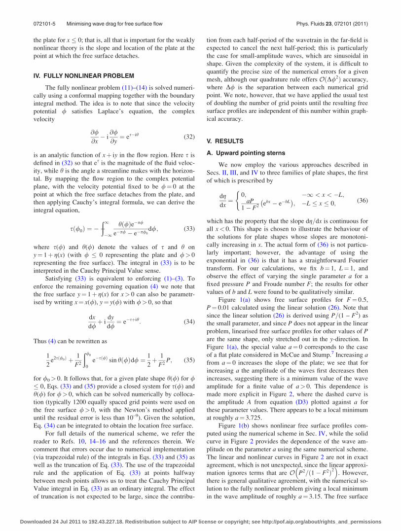
Figure 1(a) shows free surface profiles for F¼ 0.5,
P¼ 0.01 calculated using the linear solution (26). Note that
since the linear solution (26) is derived using P=(1 – F2) as
the small parameter, and since P does not appear in the linear
problem, linearised free surface profiles for other values of Pare the same shape, only stretched out in the y-direction. In
Figure 1(a), the special value a¼ 0 corresponds to the case
of a flat plate considered in McCue and Stump.7 Increasing afrom a¼ 0 increases the slope of the plate; we see that for
increasing a the amplitude of the waves first decreases then
increases, suggesting there is a minimum value of the wave
amplitude for a finite value of a> 0. This dependence is
made more explicit in Figure 2, where the dashed curve is
the amplitude A from equation (D3) plotted against a for
these parameter values. There appears to be a local minimum
at roughly a¼ 3.725.
Figure 1(b) shows nonlinear free surface profiles com-
puted using the numerical scheme in Sec. IV, while the solid
curve in Figure 2 provides the dependence of the wave am-
plitude on the parameter a using the same numerical scheme.
The linear and nonlinear curves in Figure 2 are not in exact
agreement, which is not unexpected, since the linear approxi-
mation ignores terms that are O P2=ð1� F2Þ2 �
. However,
there is general qualitative agreement, with the numerical so-
lution to the fully nonlinear problem giving a local minimum
in the wave amplitude of roughly a¼ 3.15. The free surface
072101-5 Minimising wave drag for free surface flow Phys. Fluids 23, 072101 (2011)
Downloaded 24 Jul 2011 to 192.43.227.18. Redistribution subject to AIP license or copyright; see http://pof.aip.org/about/rights_and_permissions
profiles in Figure 1(b) are plotted for values of a between
a¼ 0 and 7.15 showing that as the parameter a passes
through a¼ 3.15, the phase of the waves changes but the am-
plitude does not vanish.
We find the free surface profiles in Figure 1(b) have the
interesting property that they all appear to intersect the wave
of minimum amplitude (which happens to be for the parame-
ter value a¼ 3.15) at the waves’ troughs and crests. Thus, as
we increase the parameter a, Figure 1(b) provides an instruc-
tive example of how a family of wavetrains can have local
minimum in the wave amplitude without passing through a
waveless solution.
For completeness, also included in Figure 2 is a plot of
the wave amplitude A versus the parameter a computed using
the weakly nonlinear theory of Sec. III. As expected, this
curve does not agree very well with the other two at all, since
the weakly nonlinear theory is valid for 1� F� 1, while
this figure is for F¼ 0.5.
B. Stern shape of Binder10
It proves instructive to now revisit the one-parameter
stern shapes (6) considered by Binder.10 For each value of
the single parameter a, the shape of the stern is characterised
by having zero slope at the point at which the free surface
detaches. Using the weakly nonlinear theory of Sec. III,
Binder showed that by carefully choosing the value of a, a
trajectory representing the plate in phase space will terminate
at the “centre,” so that the two positive roots of Eq. (30)
coallesce, and the amplitude of the waves (given by Eq.
(31)) vanishes completely. As a comparison, Binder also
included numerical solutions to the fully nonlinear problem.
FIG. 1. (Color online) Free surface profiles drawn for the plate shape (36)
with F¼ 0.5, P¼ 0.01, b¼ 1 and L¼ 1. (a) Linear solutions with a¼ 0
(solid black), 1.5 (green dashed), 3 (red solid), and 4.5 (blue dotted). (b)
Nonlinear solutions for a¼ 0, 0.701, 1.401, 2.502, 2.802, 3.152 (blue thick),
4.153, 4.553, 5.674, 6.445, and 7.150.
FIG. 2. (Color online) The dependence of the wave amplitude A on the pa-
rameter a for the plate shape (36) with F¼ 0.5, P¼ 0.01, b¼ 1, L¼ 1. The
(red) solid curve, (black) dashed curve and (blue) dot-dashed curve corre-
spond to fully nonlinear, linear, and weakly nonlinear solutions,
respectively.
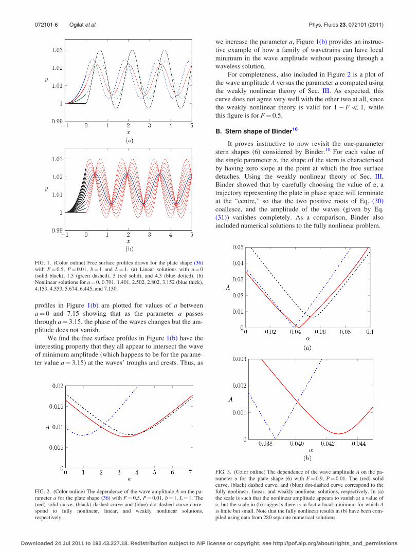
FIG. 3. (Color online) The dependence of the wave amplitude A on the pa-
rameter a for the plate shape (6) with F¼ 0.9, P¼ 0.01. The (red) solid
curve, (black) dashed curve, and (blue) dot-dashed curve correspond to the
fully nonlinear, linear, and weakly nonlinear solutions, respectively. In (a)
the scale is such that the nonlinear amplitude appears to vanish at a value of
a, but the scale in (b) suggests there is in fact a local minimum for which Ais finite but small. Note that the fully nonlinear results in (b) have been com-
piled using data from 280 separate numerical solutions.
072101-6 Ogilat et al. Phys. Fluids 23, 072101 (2011)
Downloaded 24 Jul 2011 to 192.43.227.18. Redistribution subject to AIP license or copyright; see http://pof.aip.org/about/rights_and_permissions

For the flow parameters F¼ 0.9 and P¼ 0.01 (these are
the values used by Binder10), we plot in Figure 3 the wave
amplitude versus the parameter a for the fully nonlinear, lin-
ear and weakly nonlinear cases. We see that the weakly non-
linear amplitude touches the a-axis at a¼ 0.0387, which is
the value predicted in Binder.10 However, the curve corre-
sponding to the numerical solutions to the fully nonlinear
problem appears to have a nonzero local minimum, at
a¼ 0.0427, although the actual minimum amplitude is very
small (roughly A¼ 0.0002). We note that this time the curve
for the linear solution in Figure 3 does not agree particularly
well with the numerical solutions, because while P=(1 – F2)
is reasonably small for these solutions (a requirement for the
linear theory to be valid), F¼ 0.9 is a large Froude number,
and the linear theory is known to break down as F! 1�.
To illustrate the size of the minimum wave amplitude
just mentioned, the fully nonlinear free surface profile for
a¼ 0.0427 is presented in Figure 4, together with profiles for
a¼ 0.019 and 0.0655. In Figure 4(a), we have deliberately
displayed the profiles on a scale that includes the flat bottom
of the channel, while Figure 4(b) shows the results more
clearly. We see that the profiles for a¼ 0.019 and 0.0655
have roughly the same amplitude A¼ 0.023 but are out of
phase, while the profile for a¼ 0.0427 has an amplitude that
is so small (A¼ 0.0002) the waves do not appear visible on
the scale of Figure 4(a).
It is instructive to plot a number of free surface profiles
near the wave of minimum amplitude for this family of plate
shapes. In Figure 4(c) we again the profile for a¼ 0.0427, to-
gether with six representative values of a, three greater than,
and three less than this value. As with Figure 1(b), we find
that each of these free surface profiles appears to intersect
the troughs and crests of the wave of minimum amplitude.
Thus the troughs and crests of the minimum wave act like
pivot points for the general family of profiles, demonstrating
how the wave profiles can smoothly transition between two
out of phase wavetrains without necessarily passing through
a solution that is completely flat in the far-field.
To explore this issue of eliminating waves further, we
show the relationship between wave amplitude and a for
F¼ 0.5, P¼ 0.04 in Figure 5. This parameter set is chosen
FIG. 4. (Color online) Nonlinear free surface profiles drawn for F¼ 0.9 and
P¼ 0.01 for the plate shape (6). (a) and (b) has a¼ 0.019, 0.0655 (both red)
and 0.0427 (blue and thick). (c) has a¼ 0.0393, 0.0404, 0.0416, 0.0438,
0.0450, 0.0461 (all red), and 0.0427 (blue and thick).
FIG. 5. (Color online) The dependence of the wave amplitude A on the pa-
rameter a for the plate shape (6) with F¼ 0.5, P¼ 0.04. The (red) solid
curve, (black) dashed curve, and (blue) dot-dashed curved correspond to the
fully nonlinear, linear, and weakly nonlinear solutions, respectively.
072101-7 Minimising wave drag for free surface flow Phys. Fluids 23, 072101 (2011)
Downloaded 24 Jul 2011 to 192.43.227.18. Redistribution subject to AIP license or copyright; see http://pof.aip.org/about/rights_and_permissions

so that 1 – F is no longer small, but the value of P=(1 – F2)
is roughly the same as in Figures 3 and 4. Again, we note
that for the weakly nonlinear theory, the wave amplitude
reduces to zero for some a, but the fully nonlinear solutions
have a nonzero minimum amplitude that is very small (here
the minimum amplitude is again roughly A¼ 0.0002). We
conclude that for the one-parameter family of stern shapes
(6) considered by Binder,10 the weakly nonlinear theory pre-
dicts that the wave amplitude will vanish for a single mem-
ber (corresponding to a single value of the parameter a) in
the limit F ! 1� and P=(1 – F2) ! 0. However, strictly
speaking, for 1 – F and P=(1 – F2) finite, the downstream
waves can be minimised but not entirely eliminated. The
weakly nonlinear theory of Binder10 does, of course, provide
a relatively simple and elegant way to predict what stern
shapes will generate small or large downstream waves.
C. Downward pointing sterns
Finally, motivated by studies of the analogous infinite-
depth problem,3,5,6 we generalise (6) to be (7), noting that
for b> 0 the stern has a distinctive downward-angle at the
detachment point. As with both (36) and (6), we have speci-
fied (7) so that the slope is continuous for all x. Further, the
form of (7) is easily amenable to Fourier transform, allowing
us to apply the linear theory of Sec. II.
In Figure 6 we show plots of amplitude versus b for the
same parameter values as in Figure 3. This figure shows that as
b is increased by a small amount from b¼ 0, the wave ampli-
tude decreases until a minimum is reached. In particular, for the
value a¼ 0.0427 the amplitude for b¼ 0 is A¼ 0.00019, but
the local minimum is A¼ 0.00001, which occurs for roughly
b¼ 0.001. Thus, by allowing the stern to have a very slightly
downward pointing shape at the detachment point, we are able
to reduce the (already small) minimum wave amplitude for the
shape (6) by an order of magnitude.
Figure 7 shows the dependence of amplitude versus bfor F¼ 0.5, P¼ 0.04 and a¼ 0.0527. These parameter values
correspond to the local minimum in amplitude in the fully
nonlinear case in Figure 5. Again, increasing b from b¼ 0
(at which A¼ 0.00022) introduces a slightly downward
pointing stern shape at the detachment point and we see that
for the value b¼ 0.0004 the amplitude is minimised to be
A¼ 0.00005, which is considerably small in this context.
Indeed, the free surface profile for this set of parameters is
illustrated in Figure 8, showing that effectively the wavetrain
has been eliminated entirely.
VI. DISCUSSION
It is worth summarising the three main results of the pa-
per. First, the linear free surface flow problem (11)–(14) has
mixed boundary conditions, and is therefore much more dif-
ficult to solve than the well-studied problems of flow over a
bottom topography, or flow due to a pressure distribution, for
example. Even taking into account the normal issues arising
from applying the Wiener-Hopf technique, a challenging fea-
ture of the present problem is that for plate shapes that have
slopes with compact support (dg=dx¼ 0 for x <�L with
L> 0), we are unable to close the contour of integration in
(B1) in the more natural upper half-plane, and instead have
to deal with the significant algebra that accompanies closing
the contour in the lower half-plane (note that this aspect was
not present in the flat plate problem considered by McCue
and Stump,7 since the function J(k) was identically zero in
that case). Furthermore, an additional subtlety associated
with the present problem is that the term Jþ(k) provides
the leading order behaviour in (24) for large k, being Oðk�1Þ
FIG. 6. (Color online) The dependence of the nonlinear wave amplitude Aon the parameter b for the plate shape (7) with F¼ 0.9 and P¼ 0.01. From
top to bottom, the curves are for a¼ 0.05, 0.04, and 0.0427.
FIG. 7. (Color online) The dependence of the wave amplitude A on the pa-
rameter b for the plate shape (7) with F¼ 0.5, P¼ 0.04, and a¼ 0.05268.
The (red) solid curve and (black) dashed curve correspond to the fully non-
linear and linear solutions, respectively.
FIG. 8. (Color online) Nonlinear free surface profiles drawn for F¼ 0.5 and
P¼ 0.04 for the plate shape (7) with a¼ 0.0527 and
b¼60.004, 6 0.003, 6 0.002 (all red), and 0.0004 (blue and thick).
072101-8 Ogilat et al. Phys. Fluids 23, 072101 (2011)
Downloaded 24 Jul 2011 to 192.43.227.18. Redistribution subject to AIP license or copyright; see http://pof.aip.org/about/rights_and_permissions

in the limit k ! 1, with the other term
PþðkÞm̂þðkÞ ¼ Oðk�3=2Þ. On the other hand, for the case of
the flat plate, the scalings change completely, as the function
Jþ(k) vanishes, and the term PþðkÞm̂þðkÞ transitions to being
Oðk�2Þ in the limit.
Second, the weakly nonlinear analysis of Sec. III (and
applied in other free surface flow problems in Refs. 10, 14–16)
is relatively simple to apply, and gives very good approxi-
mate solutions to the full nonlinear problem provided
1� F� 1 and P� 1. As shown by Binder,10 the theory
can be used to predict plate shapes that are candidates for
eliminating the downstream waves on the free surface. Upon
closer inspection, we find that for these plate shapes, numeri-
cal solutions to the full nonlinear equations do in fact exhibit
waves, although with such small amplitudes that the waves
are unable to be detected on a scale that includes the channel
bottom.
Third, by taking these solutions with very small wave
amplitudes, we have been able to reduce the amplitude even
further by adjusting the geometry of the plate so that it points
slightly downwards at the point of detachment (as suggested
for the infinite depth problem by3,5,6). Indeed, given the inev-
itable numerical error associated with our numerical scheme,
for these solutions we may even claim that the waves are
entirely eliminated.
Much attention in this paper has been devoted to the
question of whether or not we can adjust the shape of the
semi-infinite plate to eliminate the waves that appear on the
downstream free surface. For practical purposes, this motiva-
tion is linked to the well-known idea that there is energy
associated with wave drag behind ships, and it is desirable to
design stern shapes that minimise this energy loss by mini-
mising the wave amplitude. For free surface flow problems
in two dimensions, there is also the mathematical interest in
discovering particular subcritical solutions that are non-
generic in the sense that they exhibit free surfaces that are
flat far downstream, remembering that the general outcome
for that parameter regime is to have a train of periodic waves
on the surface in the limit. Furthermore, for configurations
that completely eliminate the waves downstream, the flow
direction can be reversed (since the radiation condition
would no longer apply), resulting in a bow flow solution. In
this case, a single (isolated) bow flow solution may also be a
member of a completely different family of solutions, such
as those with a splash near the bow, for example.
For the linearised problem of free surface flow past a
semi-infinite curved plate in a fluid of finite depth, we have
derived a (rather complicated) formula (D3) for the wave
amplitude that depends on the shape of the plate as well as
the Froude number F. For the families of plate shapes
treated in this paper, the amplitude was not eliminated, but
this does not preclude the possibility of setting up more
general families of plate shapes, and using optimisation to
eliminate the downstream waves. For the corresponding
linear problem in infinite depth, such an approach is sug-
gested by Zhu and Zhang,4 and even undertaken by
Schmidt.3 Unfortunately, as Schmidt3 does not show the
corresponding free surface profiles, it is not clear whether
his scheme actually worked.
Regardless of the results of any such linear approach,
our experience in the present study is that care must be given
to any prediction from an approximate linear or weakly non-
linear theory, as it may be that these theories predict solu-
tions without waves, when the fully nonlinear problems do
in fact exhibit waves, albeit with a very small amplitude.
Indeed, even with numerical solutions to the fully nonlinear
equations, it may appear that waves are completely elimi-
nated (as for the infinite depth problem studied by Madura-
singhe and Tuck5 and Farrow and Tuck6), when in fact they
are just too small to detect using the numerical resolution
available.
APPENDIX A: FACTORISATION OF G(k)
In McCue and Stump7 the function G(k), defined in Eq.
(19), is factorised as in Eq. (21), with
PþðkÞ ¼lRFffiffiffi
pp TðkÞC 1� ik
p
� C 3
2� ik
p
� ; (A1)
where C(z) is the usual Gamma function and T(k) is the infi-
nite product
TðkÞ ¼Y1n¼1
pln � ik
pðnþ 12Þ � ik
!:
Note that P�(k)¼Pþ(�k). Here the ln> 0 are the real posi-
tive roots to
tan pln ¼ plnF2: (A2)
The infinite product T(k) is uniformly convergent with sim-
ple zeros at k =� ipln and simple poles at k ¼ �ipðnþ 12Þ.
APPENDIX B: SPLITTING OF J(k)
1. Application of Cauchy’s integral theorem
In this Appendix we describe a key step in the analysis
of Sec. II, which is the manner that J(k), defined in Eq. (23),
is split into the sum
JðkÞ ¼ PþðkÞm̂�ðkÞ ¼ JþðkÞ þ J�ðkÞ; 0 < ImðkÞ < sþ;
where the function Jþ(k) is analytic in the upper half-plane
Im(k)> 0, while J�(k) is analytic in the lower half-plane
Im(k)< sþ. The main idea is to apply Cauchy’s integral the-
orem to give
JþðkÞ ¼1
2pi
ð1þic
�1þic
JðfÞf� k
df; (B1)
J�ðkÞ ¼ �1
2pi
ð1þid
�1þid
JðfÞf� k
df (B2)
(see Sec. 1.3 of Noble,13 for further details), where the con-
stants c and d are defined so that 0< c< Im(k)< d< sþ.
There are two possible ways to proceed, depending on
the far-field behaviour of the plate as x!�1.
072101-9 Minimising wave drag for free surface flow Phys. Fluids 23, 072101 (2011)
Downloaded 24 Jul 2011 to 192.43.227.18. Redistribution subject to AIP license or copyright; see http://pof.aip.org/about/rights_and_permissions

2. Method 1
If the slope of the plate m(x) decays continuously to
zero as x!�1 (i.e., does not have compact support), then
m̂�ðkÞ is not analytic in the upper half-plane, and will have
singularities at points denoted by jj, for j¼ 1,2,… in
Im(k)> 0 (there may be a finite number of jj). In this case,
we can close the contour in (B1) with an infinitely large
semi-circle in the upper half f-plane to give
JþðkÞ ¼ JðkÞ þX
j
Resf¼jj
JðfÞf� k
� �
¼ JðkÞ þX
j
PþðjjÞjj � k
Resf¼jj
m̂�ðfÞ:
For certain forms of m̂�ðkÞ this step could be undertaken by
inspection.
For later use, we note the far-field behaviour,
JþðkÞ � �X
j
PþðjjÞResf¼jj
m̂�ðfÞ !
1
kas k !1 (B3)
in the upper half-plane Im(k)> 0.
3. Method 2
In fact we are most interested in the case in which m(x)
does have compact support, so that m(x)¼ 0 for x <�L,
where L> 0 is some constant. Here we must be careful, as
m̂�ðkÞ is analytic everywhere, growing exponentially as k!1 in the upper half-plane Im(k)> 0. Thus we cannot close
the contour in (B1) in the upper half-plane, as the contribu-
tion from the infinitely large semi-circle would not vanish.
Instead, noting from (A1) that Pþ(k) has an infinite num-
ber of simple poles in the lower half-plane at f =� inp for
n¼ 1,2,…, we close the contour in (B1) in the lower half-
plane to give
JþðkÞ ¼ �X1n¼1
Resf¼�inp
JðfÞf� k
� �
¼X1n¼1
m̂�ð�inpÞk þ inp
Resf¼�inp
PþðfÞ: (B4)
Given that
PþðfÞ �lRFffiffiffi
pp Tð�inpÞ
Cð3=2� nÞipð�1Þn
ðn� 1Þ!ðfþ inpÞ
as f!� inp, n¼ 1,2,…, we can use the identity,
C3
2� n
� �¼
ffiffiffippð�1Þnþ1
4n�1ðn� 1Þ!ð2n� 2Þ!
to show
Resf¼�inp
PþðfÞ ¼ ilRFTð�inpÞð2n� 2Þ!
4n�1ððn� 1Þ!Þ2;
which can be substituted into (B4) to recover Jþ(k).
Again, for later use we note an alternate form for (B3) is
that
JþðkÞ �X1n¼1
m̂�ð�inpÞ ilRFTð�inpÞð2n� 2Þ!4n�1ððn� 1Þ!Þ2
!1
k(B5)
as k!1.
We now very quickly demonstrate how each of these
two methods works for the very simple example m(x)¼ aebx,
where a> 0 and b> 0 are constants. By integrating we find
m̂�ðkÞ ¼a
bþ ik;
which has a simple pole at k¼ ib. Now applying Method 1
(or by inspection) we find
JþðkÞ ¼a
bþ ikPþðkÞ � PþðibÞð Þ;
while applying Method 2 gives
JþðkÞ ¼X1n¼1
ailRF
ðbþ npÞðk þ inpÞTð�inpÞð2n� 2Þ!
4n�1ððn� 1Þ!Þ2:
In this case since m(x) decays continuously to zero as
x !�1 we can simply choose Method 1 (the simpler of
the two), but for plate shapes for which m(x) has compact
support we must choose Method 2.
APPENDIX C: DETERMINING CONSTANT C1
To solve the Wiener-Hopf equation (24) we need to con-
sider the far-field behaviour of each side of (24) as k ! 1.
To that end we note from (19) and (21) (or indeed from
(A1)) that in the upper half-plane,
PþðkÞ �il2
RF2
k
� �1=2
as k !1:
A simple application of integration by parts shows that
m̂þðkÞ �imð0Þ
kas k !1; (C1)
thus PþðkÞmþðkÞ ¼ Oðk�3=2Þ as k ! 1. However, from ei-
ther (B3) or (B5) we have JþðkÞ ¼ Oðk�1Þ, meaning that the
left-hand side of (24) is OðkÞ in the limit. As mentioned in
Sec. II, Liouville’s theorem implies that each side of (24)
must be equal to the first order polynomial C0þC1k. To
determine C1, we simply read off the leading order behaviour
from (B3) or (B5) to give
C1 ¼X
j
PþðjjÞResf¼jjm̂�ðfÞ
l2R
(C2)
or
C1 ¼ �X1n¼1
m̂�ð�inpÞ iFTð�inpÞð2n� 2Þ!lR4n�1ððn� 1Þ!Þ2
; (C3)
072101-10 Ogilat et al. Phys. Fluids 23, 072101 (2011)
Downloaded 24 Jul 2011 to 192.43.227.18. Redistribution subject to AIP license or copyright; see http://pof.aip.org/about/rights_and_permissions

depending on which method is used to close the contour in
(B1). Note that C1 is imaginary.
It is worth emphasising the difference between this anal-
ysis and that presented in McCue and Stump7 for the case of
a flat plate. In that case, when m(x)¼ 0 for all x � 0, the
function m̂�ðkÞ � 0, and so J(k) : 0. As a result, instead of
(C1) we must have m̂þðkÞ ¼ Oðk�1=2Þ, meaning that the left-
hand side of (24) would be Oð1Þ as k!1, and so each side
of (24) would be equal to a constant, C0 (i.e., C1¼ 0 for the
case of a flat plate).
APPENDIX D: INVERSE TRANSFORM
In this Appendix we evaluate the inverse transform (20)
for x> 0 by closing the path of integration with a large semi-
circle in the lower half k-plane. Given the solution for m̂ðkÞin (25), together with (A1) and either (B3) or (B5), we find
that m̂ðkÞ= tanh k has poles inside the closed contour when
k¼ 0, k¼6lR and k =� ipln for n¼ 1,2,… (where lR and
ln are defined in (16) and (A2), respectively). By summing
the appropriate residues, we find
@/1
@xðx; 1Þ ¼ �m̂ð0Þ � 1
2F2PþðlRÞP�ðlRÞ ½Pþð�lRÞðC0 þ C1lRÞe�ilRx þ PþðlRÞðC0 � C1lRÞeilRx�
þX1j¼1
�pljlRF2P�ðipljÞ1� F2 þ p2l2
j F4
C0 � C1iplj þ 1þp2l2
j
l2R
!J�ð�ipljÞ
" #e�pljx:
It is important to note that this solution is comprised of a
constant term �m̂ð0Þ, a sinusoidal term and an infinite sum
of terms that decay exponentially fast as x ! 1. Thus, by
substituting (D1) into Eq. (15), the shape of the free surface
has the behaviour
gðxÞ � P
1� F21� F2 þ F2m̂ð0Þ�
þ A sinðlRxþ �Þ
as x ! 1. But to conserve mass we want the average
value of g as x ! 1 to be P=(1 – F2), forcing the value of
m̂ð0Þ to be
m̂ð0Þ ¼ 1: (D1)
Putting it together, after some algebra, we find the shape of
the free surface is given by (26), where
A sinðlRxþ �Þ ¼ PF
1� F2
ffiffiffipp
coshðlRÞlRTðlRÞTð�lRÞ
Re TðlRÞC 1� ilR
p
� �C
3
2þ ilR
p
� �ðC0 � C1lRÞeilRx
� �;
and
BðxÞ ¼ P
1� F21þ
X1j¼1
Kje�pljx
" #; (D2)
with
Kj ¼ljlRF3TðipljÞCðljÞffiffiffi
ppð1
2þ ljÞCð12þ ljÞð1� F2 þ p2l2
j F4Þ
C0 � C1iplj þ 1þp2l2
j
l2R
!J�ð�ipljÞ
!:
A further calculation shows the amplitude to be
A ¼ FP
1� F2
ffiffiffiffiffiffiffiffiffiffiffiffiffiffiffiffiffiffiffiffiffiffiffiffiffiffiffiffiffi2ðC2
0 � C21l
2RÞ
F2 þ l2RF4 � 1
s: (D3)
We can now determine the constant C0 by substituting (D1)
in (25) to find
C0 ¼ffiffiffiffiffiffiffiffiffiffiffiffiffiffi1� F2p
� J�ð0Þ: (D4)
We see that C0 is real. Recalling that C1 is imaginary, it follows
that the wave amplitude given in (D3) vanishes only if both C0
and C1 are both zero. For the families of plate shapes consid-
ered in this study, except for the case of a flat plate, C1 was
nonzero and so the downstream waves for the linearised prob-
lem were not eliminated. For the flat plate case, C1¼ 0 but C0
was nonzero, again corresponding to waves on the free surface.
1J.-M. Vanden-Broeck, “Nonlinear stern waves,” J. Fluid Mech. 96, 603
(1980).2H. J. Haussling, “Two-dimensional linear and nonlinear stern waves,”
J. Fluid Mech. 97, 759 (1980).3G. H. Schmidt, “Linearized stern flow of a two-dimensional shallow-draft
ship,” J. Ship Res. 25, 236 (1981).4S. P. Zhu and Y. Zhang, “A flat ship theory on bow and stern flows,”
ANZIAM J. 45, 1 (2003).5M. A. Madurasinghe and E. O. Tuck, “Ship bows with continuous and splash-
less flow attachment,” J. Austral. Math. Soc. Ser. B, Appl. Math. 27, 442 (1986).6D. E. Farrow and E. O. Tuck, “Further studies of stern wavemaking,”
J. Austral. Math. Soc. 36, 424 (1995).7S. W. McCue and D. M. Stump, “Linear stern waves in finite depth
channels,” Q. J. Mech. Appl. Math. 53, 629 (2000).8S. W. McCue and L. K. Forbes, “Free-surface flows emerging from beneath a
semi-infinite plate with constant vorticity,” J. Fluid Mech. 461, 387 (2002).9M. Maleewong and R. H. J. Grimshaw, “Nonlinear free surface flows past
a semi-infinite flat plate” Phys. Fluids 20, 062102 (2008).10B. J. Binder, “Steady free-surface flow at the stern of a ship,” Phys. Fluids
22, 012104 (2010).11T. J. Osborne and D. M. Stump, “Capillary waves on a Eulerian jet emerg-
ing from a channel,” Phys. Fluids 13, 616 (2001).12V. T. Buchwald and F. Viera, “Linearised evaporation from a soil of a fi-
nite depth above a water table,” J. Austral. Math. Soc. 39, 557 (1998).13B. Noble, Methods Based on the Wiener-Hope Technique Chelsea, New
York, 1988.14B. J. Binder, J.-M. Vanden-Broeck, and F. Dias, “On satisfying the radia-
tion condition in free surface flows,” J. Fluid Mech. 624, 179 (2009).15B. J. Binder, F. Dias, and J.-M. Vanden-Broeck “Steady free surface flow
past an uneven channel bottom,” Theor. Comput. Fluid Dyn. 20, 125 (2006).16B. J. Binder, F. Dias, and J.-M. Vanden-Broeck “Influence of rapid changes in
a channel bottom on free surface flows,” IMA J. Appl. Math. 73, 254 (2008).17S. S. P. Shen, “On the accuracy of the stationary forced Korteweg-de Vries
equation as a model equation for flows over a bump,” Q. Appl. Math. 53,
701 (1995).18M. Abramowitz and I. A. Stegun, Handbook of Mathematical Functions
(Dover, New York, 1970).
072101-11 Minimising wave drag for free surface flow Phys. Fluids 23, 072101 (2011)
Downloaded 24 Jul 2011 to 192.43.227.18. Redistribution subject to AIP license or copyright; see http://pof.aip.org/about/rights_and_permissions