Miguel Adriano Koiller Schnoor The non-existence of absolutely …jairo/docs/tese_miguel.pdf ·...
80
Miguel Adriano Koiller Schnoor The non-existence of absolutely continuous invariant probabilities is C 1 -generic for flows TESE DE DOUTORADO DEPARTAMENTO DE MATEM ´ ATICA Programa de P´os-Gradua¸ c˜ ao em Matem´ atica Rio de Janeiro August 2012
Transcript of Miguel Adriano Koiller Schnoor The non-existence of absolutely …jairo/docs/tese_miguel.pdf ·...
Miguel Adriano Koiller Schnoor
The non-existence of absolutelycontinuous invariant probabilities is
C1-generic for flows
TESE DE DOUTORADO
DEPARTAMENTO DE MATEMATICA
Programa de Pos-Graduacao em Matematica
Rio de JaneiroAugust 2012
Miguel Adriano Koiller Schnoor
The non-existence of absolutely continuousinvariant probabilities is C1-generic for flows
Tese de Doutorado
Thesis presented to the Programa de Pos-Graduacao em Mate-matica of the Departamento de Matematica, PUC–Rio, as partialfulfillment of the requirements for the degree of Doutor em Ma-tematica.
Advisor: Prof. Jairo Bochi
Rio de JaneiroAugust 2012
Miguel Adriano Koiller Schnoor
The non-existence of absolutely continuousinvariant probabilities is C1-generic for flows
Thesis presented to the Programa de Pos-Graduacao em Mate-matica of the Departamento de Matematica do Centro TecnicoCientıfico da PUC–Rio, as partial fulfillment of the requirementsfor the degree of Doutor em Matematica. Approved by thefollowing commission:
Prof. Jairo BochiAdvisor
Pontifıcia Universidade Catolica do Rio de Janeiro
Prof. Alexander Eduardo Arbieto MendozaInstituto de Matematica – UFRJ
Prof. Artur Avila Cordeiro de MeloInstituo Nacional de Matematica Pura e Aplicada – IMPA
Prof. Maria Jose PacıficoInstituto de Matematica – UFRJ
Prof. Rafael Oswaldo Ruggiero RodriguezDepartamento de Matematica – PUC-Rio
Prof. Alex Lucio Ribeiro CastroDepartamento de Matematica – PUC-Rio
Prof. Martin AnderssonInstituto de MAtematica – UFF
Prof. Jose Eugenio LealCoordinator of the Centro Tecnico Cientıfico
Pontifıcia Universidade Catolica do Rio de Janeiro
Rio de Janeiro, 03/08/2012
All rights reserved.
Miguel Adriano Koiller Schnoor
B.A. and M.Sc. in Mathematics from Pontifıcia UniversidadeCatolica do Rio de Janeiro.
Bibliographic dataKoiller Schnoor, Miguel Adriano
The non-existence of absolutely continuous invariantprobabilities is C1-generic for flows / Miguel Adriano KoillerSchnoor; advisor: Jairo Bochi . — 2012.
79 f. : il. ; 30 cm
1. Tese (Doutorado em Matematica) - Pontifıcia Univer-sidade Catolica do Rio de Janeiro, Rio de Janeiro, 2012.
Inclui bibliografia
1. Matematica – Teses. 2. Fluxo de frames ortonormais;.3. probabilidade invariante absolutamente contınua;. 4. teoriaergodica;. 5. torre de Rokhlin nao invariante.. I. Bochi,Jairo. II. Pontifıcia Universidade Catolica do Rio de Janeiro.Departamento de Matematica. III. Tıtulo.
CDD: 510

In memory of my father. His incredible wisdom and irresistible tendernesscontinue to inspire me.
Acknowledgments
Foremost, I would like to express my gratitude to my advisor, Jairo Bochi,
for his patience, motivation and for all knowledge that has been passed to me
during the writing of this work. It was a huge privilege to work alongside him.
I would like to thank Capes and CNPq for the financial support that
allowed me to devote myself exclusively to the Ph.D work.
To all my family, especially my mother and my sisters, for giving me
support and love throughout my life; also to my uncle Jair and cousin Jose,
who inspired me to follow this path.
My sincere thanks also goes to Flavio Abdenur, who enthusiastically
encouraged me to study Dynamical Systems and to Lorenzo Dıaz for intro-
ducing me to this field of Mathematics. To Enrique Pujals, for his guidance
during IMPA seminars, to Alexander Arbieto and Martin Andersson, for the
many mathematical conversations, and to Thomas Lewiner, for helping me
with LATEX issues.
I was lucky to work among several incredible friends in PUC and I am
grateful not only for their suggestions and encouragement to my work, but
also for the laughs during lunch and coffee time. In special, I thank Luiz
Felipe Nobili, Rodrigo Pacheco, Yuri Ki, Debora Mondaini, Victor Goulart,
Tiane Marcarini, Eduardo Telles, Americo Barbosa, Andre Zaccur, Guilherme
Frederico Lima, Joao Paulo Romanelli, Jose Gondin, Marcio Telles, Andre
Carneiro, Wilson Reis e Bernardo Pagnoncelli.
I owe my gratitude also to students from other institutions, like Romulo
Rosa, Jaqueline Rocha, Mariana Pinheiro, Tiago Catalan, Yuri Lima, Pablo
Guarino, Pablo Barrientos, Arten Raibekas, Ivana Latosinski, Fernando Car-
neiro and Michel Cambrainha, with whom I had the opportunity to exchange
great experiences at conferences and seminars I attended.
I must put on record my admiration and appreciation for the staff of the
Mathematics Department of PUC. Without their daily help, this paper would
be impossible to exist. Above all, I must especially thank my great heroine,
Creuza.
I obviously need to thank my two loves, Sabrina and Valentina, for giving
a new - and wonderful - direction to my life.
Abstract
Koiller Schnoor, Miguel Adriano; Bochi, Jairo. The non-existenceof absolutely continuous invariant probabilities is C1-generic for flows. Rio de Janeiro, 2012. 79p. Tese de Doutorado— Departamento de Matematica, Pontifıcia Universidade Catolicado Rio de Janeiro.
We prove that C1-generic vector fields in a compact manifold do not have
absolutely continuous invariant probabilities. This extends a result of Avila
and Bochi to the continuous time case.
KeywordsAbsolutely continuous invariant probability; ergodic theory; non-
invariant Rokhlin tower; orthonormal frame flow.
Resumo
Koiller Schnoor, Miguel Adriano; Bochi, Jairo. Fluxos C1-genericos nao possuem probabilidades invariantes absolu-tamente contınuas. Rio de Janeiro, 2012. 79p. Tese de Doutorado— Departamento de Matematica, Pontifıcia Universidade Catolicado Rio de Janeiro.
Provamos que campos de vetores C1-genericos em uma variedade compacta
nao possuem probabilidades invariantes absolutamente contınuas em relacao
a uma medida de volume. Este trabalho estende ao caso de tempo contınuo
um resultado de Avila e Bochi.
Palavras–chaveFluxo de frames ortonormais; probabilidade invariante absolutamente
contınua; teoria ergodica; torre de Rokhlin nao invariante.

Contents
1 Introduction 10
1.1 Absolutely continuous invariant probabilities 10
1.2 Main Theorem 11
1.3 Remarks about the proof 11
1.4 Structure of the work 12
2 Preliminaries 15
2.1 Basic facts about vector fields and flows 15
2.2 Non-Conformality 21
2.3 Linear Cocycles 22
2.4 The orthonormal frame flow 27
2.5 Basic facts about volume crushing 28
2.6 Functions with bounded logarithmic derivative 30
2.7 Vitali Covering 32
3 Transverse Section 34
4 Tubular Chart 39
5 Local Crushing 52
5.1 Crushing-Time 54
5.2 Sliced Tube 57
5.3 Bump Function 64
5.4 Proof of the Fettuccine’s Lemma 68
6 Global Crushing 74
List of Figures
2.1 Non-compatible cross-sections. 162.2 The image of an Euclidean ball by a linear invertible map L is
incribed in a sphere with radius r2 = ‖L‖r and circumscribed ona sphere with radius r1 = ‖L−1‖−1r. 22
2.3 A linear cocycle over the flow {ϕt}. 23
3.1 A saddle p with dimW sloc(p) = 2 and dimW u
loc(p) = 1; the cross-sections Σu and Σs are respectively a cylinder and a union of twodisks. 35
4.1 Tubular Chart 414.2 Choice of the initial orthonormal frame for d = 3. 434.3 The manifold H as a graph 454.4 The 1-codimensional submanifold H = {(x,w, y) : y = xw2}
in Example 4.0.18 is graph of a function with unbounded secondderivative. 50
5.1 Schematic illustration of V being crushed. 535.2 Crushing in the y-direction. 555.3 Distortion in the w-direction is not significant if the initial slice is
thin enough. 605.4 |τs(p)− s| < ∆ for all s ∈ [a, T + ∆]. 62
1Introduction
Throughout the text, let M be a smooth compact Riemannian manifold
without boundary, and let m be the normalized Riemannian volume. The space
of all Cr vector fields on M endowed with the Cr topology will be denoted
by Xr(M). The flow induced by a vector field X ∈ X1(M) will be denoted
by {ϕtX}t∈R or simply {ϕt}t∈R if the generating vector field is clear from the
context. Let acip stand for absolutely continuous invariant probability, where
absolute continuity is understood with respect to the volume measure m.
1.1Absolutely continuous invariant probabilities
The main aspect of invariant probabilities is that they reflect the asymptotical
behavior of almost every point with respect to those measures. Although the
Krylov-Bogolubov Theorem guarantees the existence of invariant probabilities
for compact metrizable spaces, it does not give any other information about the
measure. The invariant measure on a Riemannian manifold could be singular
to respect to the Riemannian volume. On the other hand, if an invariant
probability is absolutely continuous with respect to a volume measure, then it
is guaranteed that it reflects the asymptotical behavior of points in a set with
positive volume.
The problem of dealing with acips is that, except for the case of C1+α
expanding maps (which always admit an acip), it is not known of any other
system for which the existence of acips is open (in any topology). Even in
the context of expanding maps, it was shown by A. Quas ([Q]) in dimension
one and generalized by Avila and Boch in any dimension ([AB1]), that C1-
generic invariant probabilities are singular. Avila and Bochi also generalized
Quas result (in the one dimensional case) for σ-finite measures ([AB2]). In
the space of Ck Anosov Systems, the absence of acips is an open and dense
property. This follows from the Livsic periodic orbit criterion (See [L]).
Chapter 1. Introduction 11
1.2Main Theorem
In this work we extend the result of [AB1] for C1 flows. Let us state precisely
the theorem we prove.
Theorem 1.2.1 There exists a C1-residual subset R ⊂ X1(M) such that if
X ∈ R, then X has no acip.
Notice that we are not assuming any regularity on the density of the
acip, other then integrability. If we ask the acip to be smooth or even holder-
continuous, the proof might be much simpler. Our strategy (like in [AB1]) does
not need to use these stronger hypotheses.
We assume that M has dimension d ≥ 3. There is no loss of generality
to do so, since the 2-dimensional case is a consequence of the fact that
Morse-Smale systems cannot admit an acip (Remark 2.5.3) and the following
celebrated result:
Theorem 1.2.2 (Peixoto, Pugh) Let M be a compact surface. The set of
all Morse-Smale systems is (open and) dense in X1(M).
This theorem was proved for orientable surfaces (and a few non-orientable
ones) by M. Peixoto (actually in any Cr topology), and then for every surface
(in the C1 topology) by C. Pugh, using the Closing Lemma. See [PdM,
Chapter IV].
Peixoto’s original result points to the possibility that the lack of acips
might be generic even in higher topologies, since it implies that this is true at
least for orientable surfaces.
1.3Remarks about the proof
The idea of the proof is similar to [AB1]. We consider for each δ ∈ (0, 1), the
set
Vδ ={X ∈ X1(M) : there exist a Borel set K ⊂M and T ∈ R such that
m(K) > 1− δ and m(ϕTX(K)) < δ}
These sets are clearly open (as shown in Remark 2.5.4); thus if we prove that
they are C1 dense, then the set
R ≡⋂
δ∈Q∩(0,1)
Vδ
Chapter 1. Introduction 12
will be a residual set. The fact that a vector field in R does not admit an
acip is a direct consequence of Lemma 2.5.1. We say that a vector field is δ-
crushing if X ∈ Vδ. All our effort in this work is to prove that δ-crushing is a
dense property. Thus we begin with an arbitrary X ∈ X1(M) and a constant
δ ∈ (0, 1) and show how to construct a perturbation of X with the δ-crushing
property.
The strategy to prove denseness of Vδ has two main parts. First, we show
how to construct a perturbation of X supported on a tubular neighborhood of
a very long segment of orbit in a way that the δ-crushing property with respect
to the normalized volume can be verified inside this neighborhood. This is the
content of the Fettuccine’s Lemma (Lemma 5.0.22).
The next step is to show that we can cover the manifold (except for a
negligible measure set) with “crushable” sets, permitting us to construct the
perturbation globally and, consequently, to obtain the δ-crushing property with
respect to the volume of the whole manifold. This is done by a combination of
Lemma 3.0.6, where we construct a transverse section and a first return map
with some nice properties, and Lemma 6.0.2, which gives us a Rokhlin-like
tower with respect to that first return map.
Although the general idea of the proof follows [AB1], there are some
difficulties in adapting the proof to the continuous-time case. In both cases,
the crushing is done in one dimension only, making d-dimensional objects
essentially (d − 1)-dimensional. In the continuous case, the choice of the
crushing direction and the construction of the perturbation is done with the
help of a tubular chart with several technical properties (Theorem 4.0.15),
while in the discrete setting, an atlas is fixed with the only requirement that
charts on the atlas take the volume in M to the Lebesgue measure in Rd.
In [AB1], the crushable sets are contained in a discrete open tower and
it is possible, in that case, to make ‘a priori’ adjustments, like a linearizing
perturbation of the map in each level of the tower or a rotation of coordinates
that makes Rd−1×{0} invariant by the linear perturbed map. Moreover, these
adjustments make the discrete version of Fettuccine’s Lemma ([AB1, Lemma
3]) much simpler, since the lemma needs only to give a crushing perturbation
of a sequence of linear isomorphisms.
1.4Structure of the work
In Section 2, we present some basic background which will be used throughout
the text. In §2.1, we give a slightly more general definition of Poincare maps
and present a change of coordinates that straightens the local stable and
Chapter 1. Introduction 13
unstable manifolds around a hyperbolic saddle, with the additional property
that the Euclidean norm in this coordinate system is adapted, that is, the
flow presents immediate hyperbolic contraction (resp., expansion) in the stable
(resp., unstable) coordinate. These adapted coordinates are used in the proof of
the existence of singular flow boxes around hyperbolic saddles (Lemma 3.0.7).
In §2.3, we make some remarks about linear cocycles, specially about one
specific cocycle that plays a major role in the proof of our result - the linear
Poincare flow. We give also an example of a nonlinear cocycle - the orthonormal
frame flow - which is a main tool in the construction of the tubular chart
in Section 4. We have already mentioned that the non-existence of acips is
equivalent to a volume crushing property. In §2.5, we state and prove this
criterion, with some important observations about volume crushing. In §2.6,
we prove a lemma about integrals of functions with bounded logarithmic
derivative which is used to proof that, for long tubular neighborhoods, the
volume concentrated on the edges are relatively small. As in [AB1], we need
to use the Vitali covering theorem to guarantee that, except for a small set,
we can cover the manifold with crushable sets. In §2.7, we make a precise
definition of Vitali Coverings and state this theorem.
In Section 3, as mentioned above, we prove the existence of a singular flow
box around a hyperbolic saddle (Lemma 3.0.7) and use this lemma to construct
a transverse section with the property that every point in the manifold not
contained in the stable manifold of a sink (resp. the unstable manifold of a
source) must hit the section for the future (resp. for the past).
Section 4 is devoted to prove the existence of a C2 tubular chart which
enable the construction of the perturbation in Rd. The chart has several natural
properties and some technical ones. Before the proof of Theorem 4.0.15 we give
some informal explanation about this properties and how they help us in the
construction of the perturbation.
We have already made some remarks about the Fettuccine’s Lemma,
which gives us a perturbation of the vector field inside a long tubular neigh-
borhood. Besides the tubular chart, the proof of this lemma needs several other
ingredients and Section 5 is all devoted to present those tools and proving the
Lemma (the proof is given only in § 5.4). In §5.1 we give, in Lemma 5.1.2, an
explicit formula for the time t0 = t0(ε, δ) that must elapse for an ε-perturbation
generate a δ-crushing property. We call this amount of time the crushing-time.
As in [AB1], the “size” T > 0 of the tubular neighborhood which supports
the perturbation (in that case, the height n of the open tower) must be much
bigger than the crushing-time. The reason is that the end of the crushable set
(with size less than t0) cannot be crushed. However, taking T � t0, we guar-
Chapter 1. Introduction 14
antee that the relative volume of the non-crushed part is sufficiently small.
In §5.2 we define the sliced tubes, a type of tubular neighborhood saturated
by orthogonal cross-sections which are related to the Linear Poincare Flow.
These sets are convenient to work with for many reasons. They are not bent
in the direction of the flow, for example, and their volumes are easily com-
puted. Proposition 5.2.7 shows that we can approximate a standard tubular
neighborhood by sliced tubes and in §5.3 we show how to construct a bump
function with bounded C1-norm inside a sliced tube. Finally, in Section 6, we
extend the local crushing property to the whole manifold, proving that it is
possible to cover the manifold (except for a small set) with crushable sets given
by Lemma 5.0.22.
2Preliminaries
In this section we collect several standard definitions and facts from Linear
Algebra, Differential Topology and Dynamical Systems that will be used later.
2.1Basic facts about vector fields and flows
One important tool in the analysis of the local structure of periodic orbits is
the Poincare first return map, a discrete dynamical system defined in a cross
section that inherits local properties of the flow close to a periodic orbit. In
this work we use a more general definition of the Poincare map, which allows
the map to be a first hit map between two cross sections. We also allow the
cross sections to be general codimension 1 submanifolds with boundary. It is
convenient to impose a certain compatibility condition on those submanifolds:
Definition 2.1.1 (compatibility) Given X ∈ X1(M) and its induced flow
{ϕt}t, we say that two codimension 1 submanifolds with boundary Σ1 and Σ2
are compatible if their union is still a submanifold with boundary, if they are
both transverse to X and the following holds:
inf{t > 0 : ϕt(x) ∈ Σ2} ≤ inf{t > 0 : ϕt(x) ∈ Σ1}, ∀x ∈ Σ1 (2.1)
inf{t > 0 : ϕ−t(y) ∈ Σ1} ≤ inf{t > 0 : ϕ−t(y) ∈ Σ2}, ∀y ∈ Σ2. (2.2)
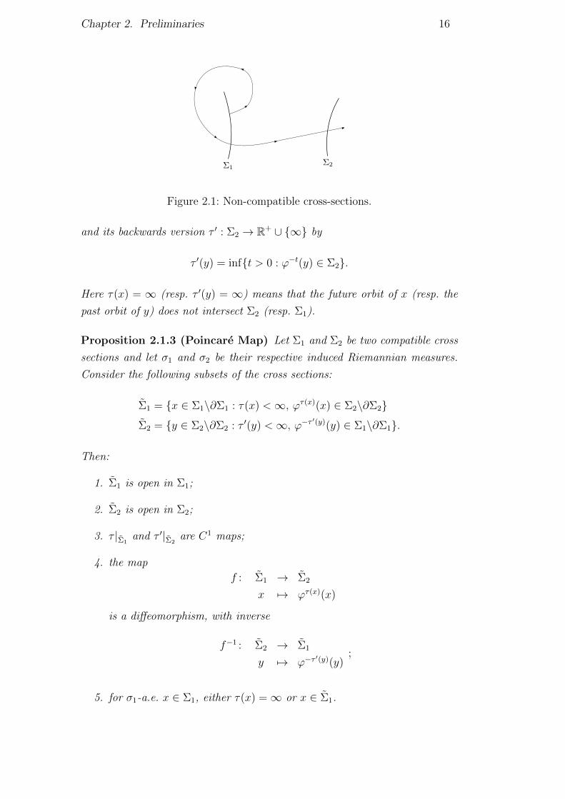
So compatibility forbids the situation of Figure 2.1. Also, note that the
above definition does not exclude the possibility of Σ1 being equal to Σ2, since
we want to consider the Poincare first return map as a particular case of the
map we are about to construct.
Definition 2.1.2 (hitting-time) Let Σ1 and Σ2 be compatible cross sections.
Then we define the hitting-time function τ : Σ1 → R+ ∪ {∞} by
τ(x) = inf{t > 0 : ϕt(x) ∈ Σ2}
Chapter 2. Preliminaries 16
Figure 2.1: Non-compatible cross-sections.
and its backwards version τ ′ : Σ2 → R+ ∪ {∞} by
τ ′(y) = inf{t > 0 : ϕ−t(y) ∈ Σ2}.
Here τ(x) = ∞ (resp. τ ′(y) = ∞) means that the future orbit of x (resp. the
past orbit of y) does not intersect Σ2 (resp. Σ1).
Proposition 2.1.3 (Poincare Map) Let Σ1 and Σ2 be two compatible cross
sections and let σ1 and σ2 be their respective induced Riemannian measures.
Consider the following subsets of the cross sections:
Σ1 = {x ∈ Σ1\∂Σ1 : τ(x) <∞, ϕτ(x)(x) ∈ Σ2\∂Σ2}
Σ2 = {y ∈ Σ2\∂Σ2 : τ ′(y) <∞, ϕ−τ ′(y)(y) ∈ Σ1\∂Σ1}.
Then:
1. Σ1 is open in Σ1;
2. Σ2 is open in Σ2;
3. τ |Σ1and τ ′|Σ2
are C1 maps;
4. the map
f : Σ1 → Σ2
x 7→ ϕτ(x)(x)
is a diffeomorphism, with inverse
f−1 : Σ2 → Σ1
y 7→ ϕ−τ′(y)(y)
;
5. for σ1-a.e. x ∈ Σ1, either τ(x) =∞ or x ∈ Σ1.
Chapter 2. Preliminaries 17
Proof: Parts 1, 2 and 3 are easy consequences of the (long) flow-box theorem
(Proposition 1.1 in Chapter 3 of [PdM]). Notice that the compatibility of the
cross sections guarantees that f is one-to-one. Its inverse is given by
f−1(y) = ϕ−τ′(y)(y).
It follows from part 3 that f and f−1 are C1 maps, thus proving part 4.
For the proof of part 5, define the following subsets:
Fi =⋃t∈R
ϕt(∂Σi), (i = 1, 2).
Then Fi ⊂ M is an immersed codimension 1 submanifold transverse to Σ1.
Therefore the intersection Fi ∩ Σ1 is an immersed codimension 2 submanifold
of Σ1, and in particular it has zero σ1 measure. Noticing that x ∈ Σ1\(F1∪F2)
implies that either τ(x) = ∞ or x ∈ Σ1, the proof of the proposition is
concluded.
The diffeomorphism f : Σ1 → Σ2 defined in the previous proposition will
be called Poincare map.
Corollary 2.1.4 Let Σ1 and Σ2 be two compatible cross sections and let
f : Σ1 → Σ2 be the induced Poincare map. Then for all ε > 0 there exists
δ > 0 such that if A ⊂ Σ1 is a measurable set with σ1(A) < δ, then
m
⋃p∈A
⋃t∈[0,τ(p)]
ϕt(p)
< ε.
Proof: It suffices to note that
σ∗(A) = m
⋃p∈A
⋃t∈[0,τ(p)]
ϕt(p)
defines a measure on Σ1 which is absolutely continuous with respect to σ1.
Notice the following consequence of long flow-box theorem:
Remark 2.1.5 Let t0 > 0 and let p ∈M be a non-periodic point or a periodic
point with period bigger then t0. Suppose Σ1 and Σ2 are cross sections (i.e.,
codimension 1 submanifolds tranverse to the flow) such that p ∈ Σ1 \ ∂Σ1 and
ϕt0(p) ∈ Σ2 \ ∂Σ2. Then there exist closed neighborhoods Σ∗1 and Σ∗2 of p and
ϕt0(p) in Σ1 and Σ2 respectively that are compatible cross-sections. Moreover,
τ(x) <∞ for all x ∈ Σ∗1.
Chapter 2. Preliminaries 18
We say that the Poincare map as in Remark 2.1.5 is based on the orbit
of p with respect to the base time t0 and denote its hitting time by τX,p,t0 .
Depending on the context, the vector field X, the point p and/or the base
time t0 that define the hitting-time map with respect to a segment of orbit
will be omitted from the notation, yielding τX , τt0 or simply τ . We denote this
Poincare map by
Φt0 : Σ∗1 → Σ∗2
x 7→ Φt0(x) = ϕτ(x)(x).(2.3)
Remark 2.1.6 Since the hitting-time map is C1 and, therefore, continuous,
we have that for all ε > 0 there exists a neighborhood V ⊂ Σ∗1 of p such that
|t0 − τt0(x)| < ε
for all x ∈ V ∩ Σ∗1.
Recall that if G : U1 → U2 is a diffeomorphism and X ∈ X1(U1) is a
vector field, we define its push-forward F∗X ∈ X1(U2) by
(F∗X)(z) ≡ DG(G−1(z)) ·X(G−1(z)).
The flows of the two vector fields are conjugate by the diffeomorphism G.
In Section 3, we will consider the Poincare map with respect to some
well-chosen sections with properties. In that construction, we will make use of
“adapted” coordinates around a hyperbolic singularity (i.e., a fixed point of the
flow), which are given by next lemma. The stable (resp. unstable) index of a
hyperbolic singularity is the dimension of its stable (resp. unstable) manifold;
in particular the sum of the indices equals d = dimM .
Lemma 2.1.7 (adapted coordinates) Let X ∈ X1(M). Suppose p ∈ M is
a hyperbolic singularity of X, and let s and u be respectively the stable and
unstable indices. Then there exist
– a chart F : U → V , where U and V are open neighborhoods of p ∈ Mand 0 ∈ Rd, respectively;
– constants Λ > λ > 0;
with the following properties:
1. F (p) = 0.
2. The local stable (resp. unstable) manifold at p is mapped by F into
Rs × {0} (resp. {0} × Ru).
Chapter 2. Preliminaries 19
3. Suppose x : R→M is an orbit of the flow generated by X and I ⊂ R is
an interval such that x(I) ⊂ U . For t ∈ I, write
F (x(t)) =(ys(t), yu(t)
)with ys(t) ∈ Rs, yu(t) ∈ Ru .
Then for all t0, t1 ∈ I with t0 < t1 we have:
e−Λ(t1−t0)‖ys(t0)‖ ≤ ‖ys(t1)‖ ≤ e−λ(t1−t0)‖ys(t0)‖ , (2.4)
eλ(t1−t0)‖yu(t0)‖ ≤ ‖yu(t1)‖ ≤ eΛ(t1−t0)‖yu(t0)‖ , (2.5)
where ‖·‖ denotes Euclidean norm.
Lemma 2.1.7 is probably well-known, but being without a precise ref-
erence, we will provide a proof. We begin with the following linear algebraic
fact:
Lemma 2.1.8 Let L : Rd → Rd be a linear map without purely imaginary
eigenvalues. Let Es (resp. Eu) be the generalized eigenspace corresponding to
eigenvalues of negative (resp. positive) real part. Then there exists an “adapted”
inner product 〈·, ·〉a on Rd and constants Λ > λ > 0 such that, for all vs ∈ Es,
vu ∈ Eu we have:
〈vs, vu〉a = 0 , (2.6)
−Λ‖vs‖2a ≤ 〈Lvs, vs〉a ≤ −λ‖vs‖2
a , (2.7)
λ‖vu‖2a ≤ 〈Lvu, vu〉a ≤ Λ‖vu‖2
a . (2.8)
where ‖v‖2a = 〈v, v〉a.
Proof: First consider the case where all eigenvalues of L have negative real
part. Then the exponential matrix eL has spectral radius ρ < 1. Let ‖·‖ be the
Euclidean norm. By the spectral radius theorem (Gelfand formula), we have
limt→+∞1t
log ‖etL‖ = log ρ < 0. Therefore the following expression defines a
new norm:
‖v‖2a =
∫ ∞0
‖etL · v‖2 dt .
It is clear that this norm corresponds to an inner product 〈·, ·〉a. Notice that
s ≥ 0 ⇒ ‖esL · v‖2a =
∫ ∞s
‖etL · v‖2 dt .
In particular,d
ds
∣∣∣∣s=0
‖esL · v‖2a = −‖v‖2 .
Chapter 2. Preliminaries 20
On the other hand, the same derivative can be computed as
d
ds
∣∣∣∣s=0
〈esL · v, esL · v〉a = 2〈Lv, v〉a .
Thus 〈Lv, v〉a = −12‖v‖2, which is between −Λ‖v‖2
a and −λ‖v‖2a for some
constants Λ > λ > 0.
We proved the lemma in the particular case where all eigenvalues of L
have negative real part. The general case of the lemma follows by considering
the restrictions L|Es and (−L)|Eu and taking the orthogonal sum inner
product.
Remark 2.1.9 All inner products on Rd coincide modulo a linear change
of coordinates. Therefore, in the situation of Lemma 2.1.8 we can find an
invertible linear map S : Rd → Rd such that if L, Es and Eu are replaced with
SLS−1, S(Es), S(Eu), then the relations (2.6), (2.7), (2.8) hold with 〈·, ·〉abeing the Euclidean inner product.
Proof of Lemma 2.1.7: By changing coordinates, we can assume that the
vector field X is defined on a neighborhood of p = 0 in Rd. Let Es and Eu
denote the stable and unstable subspaces. As a trivial consequence of the
stable manifold theorem (see for example [PdM, pp.88–89]), we can change
coordinates again so that the local stable and unstable manifolds are contained
in the vector subspaces Es and Eu, respectively. By applying the linear change
of coordinates given by Remark 2.1.9, we can assume that there are constants
Λ > λ > 0 such that relations (2.6), (2.7), (2.8) hold for L = DX(0), with 〈·, ·〉abeing the Euclidean inner product. By a final change of coordinates using an
orthogonal linear map, we can assume that Es = Rs×{0} and Eu = {0}×Ru.
In coordinates (ys, yu) ∈ Rs × Ru, we write
X(ys, yu) =(Xs(ys, yu), Xu(ys, yu)
).
Then we have
Xs(ys, 0) = 0 , Xu(0, yu) = 0 .
Fix a positive ε < λ. Then for every (ys, yu) sufficiently close to (0, 0), we have
∥∥Xs(ys, yu)− L(ys, 0)∥∥ ≤ ε‖ys‖ ,∥∥Xu(ys, yu)− L(0, yu)∥∥ ≤ ε‖yu‖ .
We reduce the chart domain so that these properties are satisfied. Now assume
that t ∈ I 7→ (ys(t), yu(t)) is a trajectory of the flow contained in this chart
Chapter 2. Preliminaries 21
domain. Then
d
dt
∣∣∣∣t=0
‖ys(t)‖2 = 2⟨Xs(ys(t), yu(t)), (ys(t), 0)
⟩≤ 2(−λ+ ε)‖ys(t)‖2
This implies that the second inequality in (2.4) holds with λ− ε in the place of
λ. The remaining inequalities are proven similarly (with Λ replaced by Λ + ε).
Recall that the main part of the proof of the main result is to perturb
a given vector field so that it has the δ-crushing property. Actually we will
perform a few successive perturbations, each one preparing the ground for the
next one. In this regard, the following fact will be useful:
Proposition 2.1.10 The set I ⊂ Xr(M) of vector fields such that all periodic
orbits are hyperbolic (and isolated) is a C1-open and dense set.
Proof: This proposition is a intermediate step of the proof of the Kupka–
Smale Theorem and can be found for example in [PdM, p.115].
2.2Non-Conformality
If L is a linear isomorphism between inner-product vector spaces, the non-
conformality of L is
NC(L) ≡ ‖L‖ ‖L−1‖.
This quantity measures how much L can distort angles, in fact:
1
‖L‖ · ‖L−1‖≤ sin(∠(Lu, Lv))
sin(∠(u, v))≤ ‖L‖ · ‖L−1‖. (2.9)
See [BV, Lemma 2.7] for a proof of (2.9).
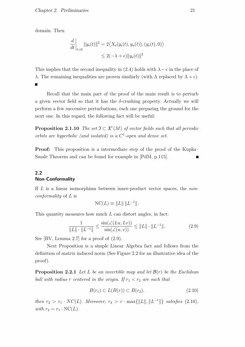
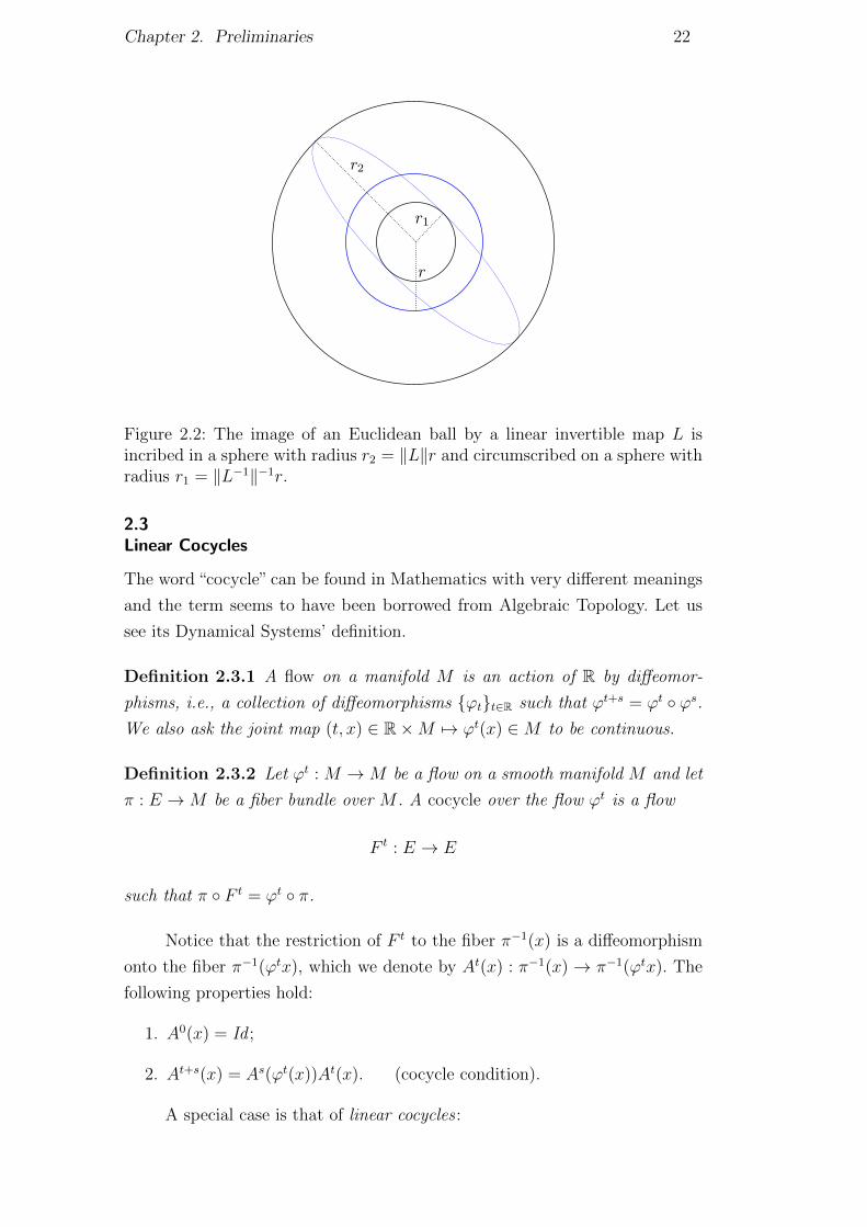
Next Proposition is a simple Linear Algebra fact and follows from the
definition of matrix induced norm (See Figure 2.2 for an illustrative idea of the
proof).
Proposition 2.2.1 Let L be an invertible map and let B(r) be the Euclidean
ball with radius r centered in the origin. If r1 < r2 are such that
B(r1) ⊂ L(B(r)) ⊂ B(r2), (2.10)
then r2 > r1 · NC(L). Moreover, r2 > r · max{‖L‖, ‖L−1‖} satisfies (2.10),
with r2 = r1 · NC(L).
Chapter 2. Preliminaries 22
Figure 2.2: The image of an Euclidean ball by a linear invertible map L isincribed in a sphere with radius r2 = ‖L‖r and circumscribed on a sphere withradius r1 = ‖L−1‖−1r.
2.3Linear Cocycles
The word “cocycle” can be found in Mathematics with very different meanings
and the term seems to have been borrowed from Algebraic Topology. Let us
see its Dynamical Systems’ definition.
Definition 2.3.1 A flow on a manifold M is an action of R by diffeomor-
phisms, i.e., a collection of diffeomorphisms {ϕt}t∈R such that ϕt+s = ϕt ◦ ϕs.We also ask the joint map (t, x) ∈ R×M 7→ ϕt(x) ∈M to be continuous.
Definition 2.3.2 Let ϕt : M →M be a flow on a smooth manifold M and let
π : E →M be a fiber bundle over M . A cocycle over the flow ϕt is a flow
F t : E → E
such that π ◦ F t = ϕt ◦ π.
Notice that the restriction of F t to the fiber π−1(x) is a diffeomorphism
onto the fiber π−1(ϕtx), which we denote by At(x) : π−1(x) → π−1(ϕtx). The
following properties hold:
1. A0(x) = Id ;
2. At+s(x) = As(ϕt(x))At(x). (cocycle condition).
A special case is that of linear cocycles :
Chapter 2. Preliminaries 23
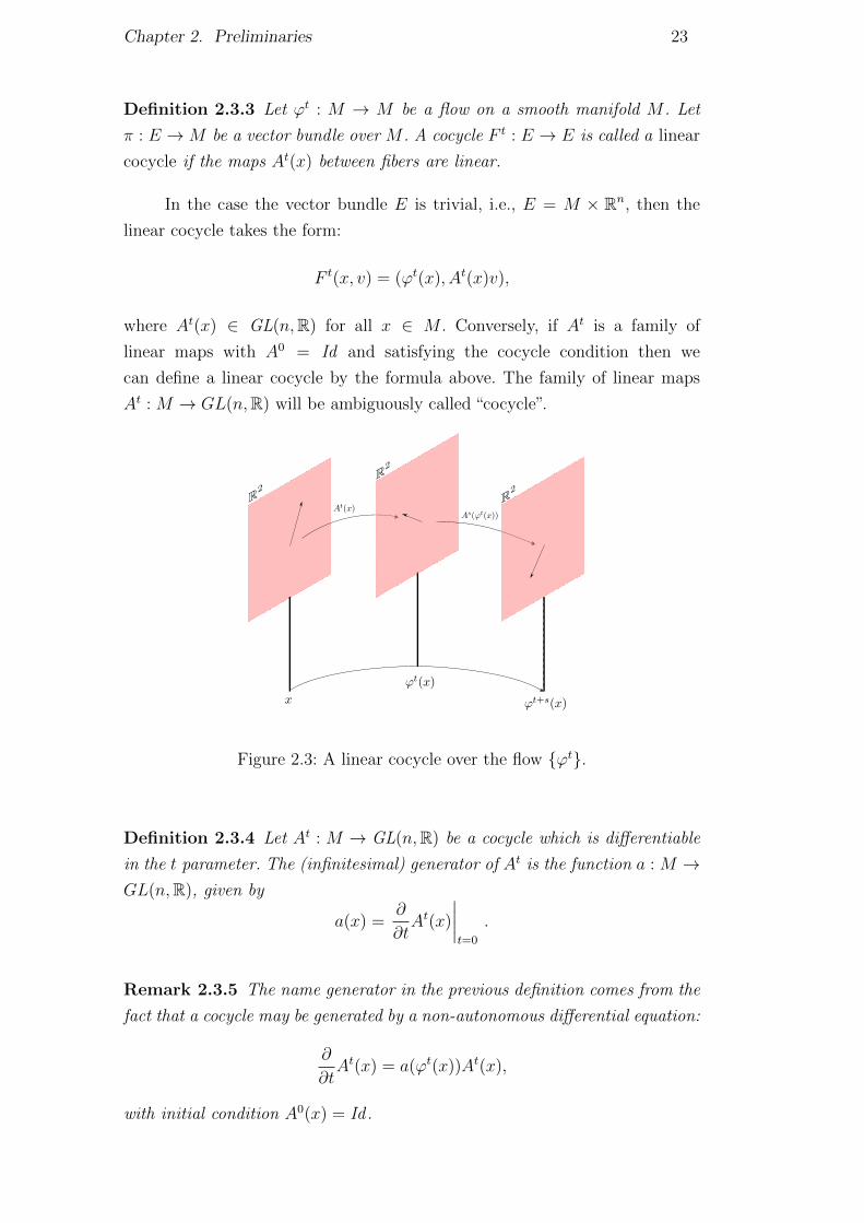
Definition 2.3.3 Let ϕt : M → M be a flow on a smooth manifold M . Let
π : E →M be a vector bundle over M . A cocycle F t : E → E is called a linear
cocycle if the maps At(x) between fibers are linear.
In the case the vector bundle E is trivial, i.e., E = M × Rn, then the
linear cocycle takes the form:
F t(x, v) = (ϕt(x), At(x)v),
where At(x) ∈ GL(n,R) for all x ∈ M . Conversely, if At is a family of
linear maps with A0 = Id and satisfying the cocycle condition then we
can define a linear cocycle by the formula above. The family of linear maps
At : M → GL(n,R) will be ambiguously called “cocycle”.
Figure 2.3: A linear cocycle over the flow {ϕt}.
Definition 2.3.4 Let At : M → GL(n,R) be a cocycle which is differentiable
in the t parameter. The (infinitesimal) generator of At is the function a : M →GL(n,R), given by
a(x) =∂
∂tAt(x)
∣∣∣∣t=0
.
Remark 2.3.5 The name generator in the previous definition comes from the
fact that a cocycle may be generated by a non-autonomous differential equation:
∂
∂tAt(x) = a(ϕt(x))At(x),
with initial condition A0(x) = Id.
Chapter 2. Preliminaries 24
Proposition 2.3.6 Let At : M → GL(n,R) be a cocycle with generator
a : M → GL(n,R). Then we have:
1. ‖At(p)‖ ≤ eC|t|;
2. ‖At(p)− Id‖ ≤ eC|t| − 1,
where C = supx∈M ‖a(x)‖.
Proof: In order to prove part 1, define f(t) = ‖At(x)‖ and note that
|f ′(t)| ≤∥∥∥∥ ∂∂tAt(x)
∥∥∥∥= ‖a(ϕt(x))At(x)‖
≤ Cf(t).
That is, |(log f(t))′| ≤ C. Since f(0) = ‖Id‖ = 1, we have f(t) ≤ eC|t|, as we
wanted to show.
The proof of part 2 is analogous. Let us now consider Bt = At−Id . Then
we have∂
∂tBt(x) = a(ϕt(x))(Id +Bt(x)).
Defining the function g(t) = ‖Bt(x)‖, we have that
|g′(t)| ≤∥∥∥∥ ∂∂tBt(x)
∥∥∥∥≤ C(1 + g(t)).
The solution of the ODE:
h′(t) = C(1 + h(t)),
h(0) = 0,
is h(t) = eCt − 1. Thus if t > 0 then g(t) ≤∫ t
0|g′| ≤ h(t) = eCt − 1, and
analogously for t < 0.
Every linear cocycle in GL(n,R) over a flow ϕt induces a cocycle in R,
by taking the determinant of the matrix At(x). The precise statement of this
well known result is given by the following proposition and its proof can be
found for example in [CL, Theorem I.7.3].
Chapter 2. Preliminaries 25
Proposition 2.3.7 Let A : R × M → GL(n,R) be a cocycle over the flow
ϕ : R × M → M with generator G : M → GL(n,R). Then the function
f : R×M → R, defined by
f(t, p) = detAt(p)
is a linear cocycle in R over the same flow. Moreover its generator g : M → Ris given by
g(p) = trG(p). (2.11)
Consider X ∈ X1(M). Let us see some natural examples of linear cocycles
over the flow ϕt generated by a vector field X. The first one is the derivative
cocycle:
TxM → Tϕt(x)M
u 7→ Dϕt(x)u,
The cocycle condition is a direct consequence of the chain rule.
The second example is the linear Poincare flow. Let R(X) ⊂ M be the
set of regular points in M , that is,
R(X) = {x ∈M : X(x) 6= 0}.
Let us define the normal bundle NR(X) associated to X. For each x ∈ R(X), let
Nx be the orthogonal complement of X(x) in TxM . This is a fiber of a vector
bundle over R(X), which is a subbundle of TR(X)M .
Definition 2.3.8 The linear Poincare flow of X is defined over NR(X) by
P tx : Nx → Nϕt(x)
u 7→ Πϕt(x) ◦Dϕt(x)u,
where Πx : TxM → Nx denotes the orthogonal projection on the normal
subbundle.
The cocycle condition of the linear Poincare flow follows from the chain
rule.
The linear Poincare flow is commonly used in the study of flows local
behavior; the reason is given by the next proposition.
Chapter 2. Preliminaries 26
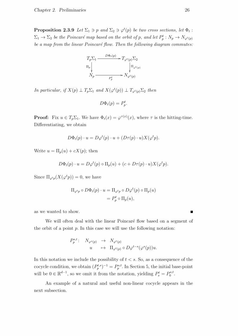
Proposition 2.3.9 Let Σ1 3 p and Σ2 3 ϕt(p) be two cross sections, let Φt :
Σ1 → Σ2 be the Poincare map based on the orbit of p, and let P tp : Np → Nϕt(p)
be a map from the linear Poincare flow. Then the following diagram commutes:
TpΣ1DΦt(p) //
Πp
��
Tϕt(p)Σ2
Πϕt(p)
��Np
P tp
// Nϕt(p)
In particular, if X(p) ⊥ TpΣ1 and X(ϕt(p)) ⊥ Tϕt(p)Σ2 then
DΦt(p) = P tp.
Proof: Fix u ∈ TpΣ1. We have Φt(x) = ϕτ(x)(x), where τ is the hitting-time.
Differentiating, we obtain
DΦt(p) · u = Dϕt(p) · u+ (Dτ(p) · u)X(ϕtp).
Write u = Πp(u) + cX(p); then
DΦt(p) · u = Dϕt(p) ◦ Πp(u) + (c+Dτ(p) · u)X(ϕtp).
Since Πϕtp(X(ϕtp)) = 0, we have
Πϕtp ◦DΦt(p) · u = Πϕtp ◦Dϕt(p) ◦ Πp(u)
= P tp ◦ Πp(u),
as we wanted to show.
We will often deal with the linear Poincare flow based on a segment of
the orbit of a point p. In this case we will use the following notation:
P s,tp : Nϕs(p) → Nϕt(p)
u 7→ Πϕt(p) ◦Dϕt−s(ϕs(p))u.
In this notation we include the possibility of t < s. So, as a consequence of the
cocycle condition, we obtain (P t,sp )−1 = P s,t
p . In Section 5, the initial base-point
will be 0 ∈ Rd−1, so we omit it from the notation, yielding P ts = P s,t
0 .
An example of a natural and useful non-linear cocycle appears in the
next subsection.
Chapter 2. Preliminaries 27
2.4The orthonormal frame flow
In Section 4, we will define a tubular chart with some useful geometrical
properties. To construct this chart, a bundle structure is necessary – the
orthonormal frame bundle. We will also need to define a special cocycle over
this bundle – the orthonormal frame flow.
Recall that M is a smooth (C∞) compact manifold of dimension d,
endowed with a Riemannian metric. For each x ∈ M , let Fx be the set of
orthonormal frames on the tangent space TxM (i.e. ordered orthonormal bases
of TxM). Let F =⊔x∈M Fx. One can define a smooth differentiable structure
on F so that the obvious projection Π : F → M is smooth and defines a fiber
bundle, whose fibers are diffeomorphic to the orthonormal group O(d). This is
called the orthonormal frame bundle of M .
There is an equivalent way of constructing this bundle: An oriented flag
at the point x ∈ M is a nested sequence F1 ⊂ F2 ⊂ · · · ⊂ Fd of vector
subspaces of TxM with dimFi = i. Given such an oriented flag, there exists
an orthonormal frame (e1, . . . , ed) such that Fi is spanned by e1, . . . , ei. This
correspondence is one-to-one and onto. Therefore F can also be viewed as a
bundle of oriented flags.
Next, fix a vector field X ∈ Xr(M), and let {ϕt}t be the induced flow
on M . Then we define a flow on F as follows: For each t ∈ R, the t-image of
the orthonormal frame (e1, . . . , ed) ∈ Fx is obtained by applying the Gram–
Schmidt process to the frame (Dϕt(x) · e1, . . . , Dϕt(x) · ed). This is called the
orthonormal frame flow. It is a flow of class Cr−1.
Using the identification between orthonormal frames and oriented flags,
the orthonormal frame flow can be described as follows: for each t ∈ R, the
t-image of the flag F1 ⊂ F2 ⊂ · · · ⊂ Fd = TxM is the flag Dϕt(x)(F1) ⊂Dϕt(x)(F2) ⊂ · · · ⊂ Dϕt(x)(Fd), where each space is endowed with the induced
orientation.
Remark 2.4.1 More generally, given any vector bundle endowed with a Rie-
mannian metric, one can define an associated orthonormal frame bundle, and
given a linear cocycle on the vector bundle, one can define an associated or-
thonormal frame flow. We will not need those more general constructions.
Chapter 2. Preliminaries 28
2.5Basic facts about volume crushing
There is a somewhat philosophical obstacle in trying to prove, in a direct way,
a theorem of nonexistence. In order to circumvent such issue we present in this
section a lemma that reduces our problem to an existence one. It is merely a
version for flows of [AB1, Lemma 1].
Lemma 2.5.1 (Criterion for non-existence of acip) A flow {ϕt} gener-
ated by a vector field X ∈ X1(M) has no acip iff for every ε > 0 there exists a
Borel set K ⊂M and T ∈ R such that
m(K) > 1− ε and m(ϕT (K)) < ε.
Proof: Notice that the validity of the lemma is unchanged if we replace
“T ∈ R” by “T ∈ R+” (just replace K by M \K), or by “T ∈ N” (because the
flow up to time 1 cannot distort volumes by more than some constant factor).
We will derive the lemma for the discrete-time version ([AB1, Lemma
1]), which says that a C1 map f : M →M has no acip iff for every ε > 0 there
exists a compact set K ⊂M and T ∈ N such that
m(K) > 1− ε and m(fT (K)) < ε.
(Compactness is useful to guarantee measurability of fT (K) even when f is
not invertible.) Notice that if we assume that f is a diffeomorphism, then using
the regularity of the measure m, we can replace “compact set” by “Borel set”
above.
Notice that a flow {ϕt} has an acip iff its time-one map ϕ1 has an acip;
indeed, if µ is an acip for ϕ1 then µ =∫ 1
0ϕt∗µ dt is an acip for the flow. Hence
the lemma follows.
For some trivial parts of the dynamics, the crushing property is auto-
matic; for example:
Remark 2.5.2 Let X ∈ X1(M). Let MS be the union all stable manifolds
of (hyperbolic) sinks and unstable manifolds of (hyperbolic) sources. If MS is
non-empty then for all ε > 0, there is a Borel set K ⊂ MS and T > 0 such
that
m(K) > m(MS)− ε and m(ϕt(K)) < ε for all t > T .
Proof: Take a small neighborhood V1 (resp. V2) of the set of sinks (resp.
sources), choose T large, and define K = ϕ−T (V1) ∪ ϕT (M \ V2).
Chapter 2. Preliminaries 29
Later on, our perturbations will be supported on the complement of MS,
because in MS there is nothing to do.
Remark 2.5.3 One could improve Remark 2.5.2 by including in MS also the
stable (resp. unstable) sets of the hyperbolic attracting (resp. repelling) periodic
orbits of X. For example, if the flow is Morse–Smale then the enlarged MS has
full Lebesgue measure, and it follows from Lemma 2.5.1 that there is no acip.
(Of course, this also follows directly from the Poincare Recurrence Theorem
and the fact that the recurrent set for a Morse–Smale flow consists of a finite
number of periodic orbits.)
As explained in the Introduction, the following property is essential to
our strategy:
Remark 2.5.4 For each ε > 0, the set
Vε ={X ∈ X1(M) : there exist a Borel set K ⊂M and T ∈ R such that
m(K) > 1− ε and m(ϕTX(K)) < ε}
is open in the C1 topology.
Proof: Let X ∈ Vε. Take a Borel set K ⊂ M and T ∈ R such that
m(K) > 1 − ε and m(ϕTX(K)) < ε. Choose a positive γ < ε − m(ϕTX(K)).
Take Y ∈ X1(M) sufficiently C1-close to X such that
| det(DϕTX(p))− det(DϕTY (p))| < γ
m(K),
for all p ∈M . Then we obtain that
m(ϕTY (K)) =
∫K
| det(DϕTY (p))|dm(p)
<
∫K
(| det(DϕTX(p))|+ γ
m(K)
)dm(p)
= m(ϕTX(K)) + γ < ε.
And we conclude that Y ∈ Vε.
Lemma 2.5.1 and Remark 2.5.4 together imply that that the non-
existence of acip is a Gδ property.
Chapter 2. Preliminaries 30
2.6Functions with bounded logarithmic derivative
Recall that the logarithmic derivative of a positive function f(s) is
(log(f(s)))′ = f ′(s)/f(s).
A simple consequence of the boundedness of the logarithmic derivative
is that, in this case, the function presents sub-exponential growth.
Remark 2.6.1 (Sub-exponential growth) Let b > 0 and f : R → R be a
positive function such that∣∣∣∣ dds(log(f(s)))
∣∣∣∣ < b, ∀s ∈ R.
Then
e−b|s| < f(s) < eb|s|, ∀s ∈ R.
Let I = [α, β] ⊂ R be a compact interval and let a > β − α. We will use
the following notation:
Ia ≡ [α + a, β − a] and Ia ≡ [α− a, β + a].
Proposition 2.6.2 Given b > 0, t0 > 0 and γ ∈ (0, 1), there exists a0 > 0
such that for all 0 < a < a0, for any interval I with |I| > t0 and for all positive
f ∈ C1(R,R) such that
|f ′(s)| ≤ bf(s), ∀s ∈ R
the following holds: ∫Ia
f(s)ds > (1− γ)
∫Iaf(s)ds.
Before proving this proposition, we need a lemma:
Lemma 2.6.3 Let f and b be as in the previous Proposition. Then given
α < β, we have that
b−1 max{f(α), f(β)}(1−e−b(β−α)) <
∫ β
α
f(s)ds < b−1 min{f(α), f(β)}(eb(β−α)−1).
Proof: Let α < t < β. By the hypothesis’ inequality,
b >
∣∣∣∣f ′(s)f(s)
∣∣∣∣ , (2.12)
Chapter 2. Preliminaries 31
for all s ∈ R. Integrating both sides from α to t, we obtain
b(t− α) >
∫ t
α
∣∣∣∣f ′(s)f(s)
∣∣∣∣ ds>
∣∣∣∣∫ t
α
f ′(s)
f(s)ds
∣∣∣∣=
∣∣∣∣log
(f(t)
f(α)
)∣∣∣∣ .Which leads us to
f(α)e−b(t−α) < f(t) < f(α)eb(t−α). (2.13)
If we integrate both sides of (2.12) from t to β we will obtain a similar
conclusion:f(β)e−b(β−t) < f(t) < f(β)eb(β−t). (2.14)
Using the righthand side of both (2.13) and (2.14) we conclude that∫ β
α
f(t)dt < b−1 min{f(α), f(β)}(eb(β−α) − 1).
The same way, using the lefthand side of (2.13) and (2.14) we get∫ β
α
f(t)dt > b−1 max{f(α), f(β)}(1− e−b(β−α)).
Proof of Proposition 2.6.2: Let
a0 = min
{t02, (2b)−1 log
(γ
(1− e−bt0)2
+ 1
)}and assume that I = [α, β], with |β − α| < t0. Take 0 < a < a0 and T > t0
and denote
A =
∫ β+a
α−af(s)ds.
Our goal is to prove that∫ α+a
α−af(s)ds < (γ/2)A and
∫ β+a
β−af(s)ds < (γ/2)A.
Since the proofs of both inequalities are totally analogous, we present only the
the proof of the first one.
Chapter 2. Preliminaries 32
From Proposition 2.6.2 and the fact that |β − α| < t0 we have that
A ≥ b−1 max{f(α− a), f(β + a)}(1− e−b(t0+2a))
≥ b−1f(α− a)(1− e−b(t0+2a)). (2.15)
Again from Proposition 2.6.2, we obtain∫ α+a
α−af(s)ds ≤ b−1 min{f(α− a), f(α + a)}(e2ba − 1)
≤ b−1f(α− a)(e2ba − 1). (2.16)
From Inequalities (2.15), (2.16) and the fact that 0 < a < a0, we conclude that∫ α+a
α−af(s)ds ≤ A(e2ba − 1)
1− e−b(t0+2a)
<A(e2ba − 1)
1− e−bt0
< Aexp(log(γ(1−e−bt0 )
2+ 1))− 1
1− e−bt0
= Aγ(1−e−bt0 )
2
1− e−bt0
= Aγ
2.
2.7Vitali Covering
In this work, we use a version of the Vitali Covering Theorem (usually stated in
Rd) for compact Riemannian manifolds and include the possibility of the sets
in the covering not being balls for the Riemannian metric. For the Theorem
still hold in this more general setting, we need that the sets in the cover satisfy
a roundness property. Roughly speaking, this property means that the sets
can be sandwiched by balls for which the ratio between the radii is uniformly
bounded. This property is defined in [P, Appendix E].
Definition 2.7.1 (Quasi-roundness) Let M be a Riemannian Manifold and
x ∈ M . We say that U ⊂ M is a K-quasi-round neighborhood of x if there
Chapter 2. Preliminaries 33
exists r > 0 (lower then the injective radius) such that
BK−1r(x) ⊂ U ⊂ Br(x),
where Br(x) is the Riemannian ball around x with radius r.
Definition 2.7.2 (Vitali Cover) Let S ⊂ M and let K > 1. If V = {Vα}is a cover of S such that for m-a.e. x ∈ S and for all r ∈ (0, supα diam(Uα))
there exists a K-quasi-round neighborhood U ⊂ V of x with U ⊂ Br(x), then
we say that V is a Vitali Cover of S.
Theorem 2.7.3 (Vitali Covering Theorem) If V is a Vitali cover of S,
then there exists a countable pairwise disjoint family {Vj}j ⊂ V such that
m
(S\⋃j
Vj
)= 0.
Proposition 2.7.4 Let M and N be compact Riemannian manifolds and let
F : U ⊂ M → F (U) ⊂ N be a diffeomorphism with uniform bounded non-
conformality, that is, there exists C > 1 such that
NC(DF (p)) < C, ∀p ∈ U.
Then for all x ∈ U , there exists r > 0 such that for all K-quasi-round neigh-
borhood V 3 x with diam(V ) < r, F (V ) is a KC-quasi-round neighborhood of
F (x).
Proof: Since we can take V arbitrarily small, the proof follows from Propo-
sition 2.2.1.
Remark 2.7.5 We conclude, by the previous Proposition and Theorem 2.7.3,
that Vitali Covers are preserved by diffeomorphisms with uniform bounded non-
conformality.
3Transverse Section
In this section, we show that for a C1 open and dense subset of X1(M), we can
construct a transverse section and a return map with some properties (Lemma
3.0.6) that will permit us to use, in Section 6, a non-invariant Rokhlin lemma
(Lemma 6.0.2) to obtain a disjoint finite union of tubular neighborhoods that
cover M , except for a set of negligible Lebesgue measure.
Recall that a cross-section for a flow is a codimension 1 closed submani-
fold with boundary that is transverse to the vector filed.
Lemma 3.0.6 Let X ∈ X1(M) be a vector field with only hyperbolic singular-
ities. Then there exists a cross-section Σ ⊂M such that:
1. if x ∈ M does not belong to a stable manifold of a sink or saddle
singularity then the future orbit of x hits Σ;
2. if x ∈ M does not belong to an unstable manifold of a source or saddle
singularity then the past orbit of x hits Σ.
Before showing how to construct the cross-section Σ, we will prove an
intermediate step, which gives the appropriate cross-sections in the neighbor-
hood of a saddle-type singularity.
Lemma 3.0.7 (singular flow-box) Let p be a hyperbolic singularity of X ∈X1(M) of saddle type. Then there exist compatible cross-sections Σu and Σs
with the following properties:
1. If f : Σu → Σs is the Poincare map given by Proposition 2.1.3, then
Σu = Σu \ ∂Σu \W sloc(p),
Σs = Σs \ ∂Σs \W uloc(p).
2. Letting τ be the associated hitting-time, the set
V =⋃x∈Σu
⋃t∈[0,τ(x)]
ϕt(x), (3.1)
is a closed neighborhood of the saddle p.
Chapter 3. Transverse Section 35
3. For any point x ∈M \V , if the future (resp. past) orbit of x hits V then
the first hit is in Σu (resp. Σs).
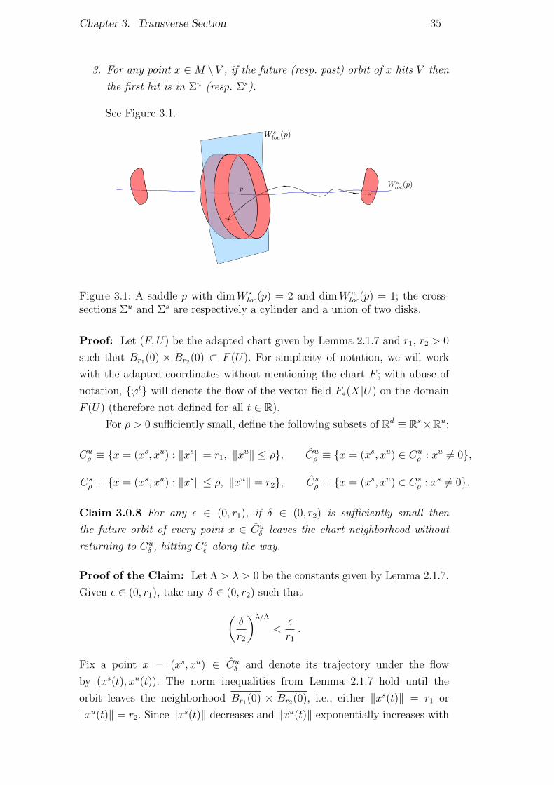
See Figure 3.1.
Figure 3.1: A saddle p with dimW sloc(p) = 2 and dimW u
loc(p) = 1; the cross-sections Σu and Σs are respectively a cylinder and a union of two disks.
Proof: Let (F,U) be the adapted chart given by Lemma 2.1.7 and r1, r2 > 0
such that Br1(0) × Br2(0) ⊂ F (U). For simplicity of notation, we will work
with the adapted coordinates without mentioning the chart F ; with abuse of
notation, {ϕt} will denote the flow of the vector field F∗(X|U) on the domain
F (U) (therefore not defined for all t ∈ R).
For ρ > 0 sufficiently small, define the following subsets of Rd ≡ Rs×Ru:
Cuρ ≡ {x = (xs, xu) : ‖xs‖ = r1, ‖xu‖ ≤ ρ}, Cu
ρ ≡ {x = (xs, xu) ∈ Cuρ : xu 6= 0},
Csρ ≡ {x = (xs, xu) : ‖xs‖ ≤ ρ, ‖xu‖ = r2}, Cs
ρ ≡ {x = (xs, xu) ∈ Csρ : xs 6= 0}.
Claim 3.0.8 For any ε ∈ (0, r1), if δ ∈ (0, r2) is sufficiently small then
the future orbit of every point x ∈ Cuδ leaves the chart neighborhood without
returning to Cuδ , hitting Cs
ε along the way.
Proof of the Claim: Let Λ > λ > 0 be the constants given by Lemma 2.1.7.
Given ε ∈ (0, r1), take any δ ∈ (0, r2) such that(δ
r2
)λ/Λ<
ε
r1
.
Fix a point x = (xs, xu) ∈ Cuδ and denote its trajectory under the flow
by (xs(t), xu(t)). The norm inequalities from Lemma 2.1.7 hold until the
orbit leaves the neighborhood Br1(0) × Br2(0), i.e., either ‖xs(t)‖ = r1 or
‖xu(t)‖ = r2. Since ‖xs(t)‖ decreases and ‖xu(t)‖ exponentially increases with
Chapter 3. Transverse Section 36
t, there exists T > 0 such that ‖xu(T )‖ = r2. Using (2.5) in Lemma 2.1.7, we
have
r2 = ‖xu(T )‖ ≤ eΛT · ‖xu(0)‖ = eΛT δ,
which leads us to
T >1
Λlog(r2
δ
).
From the choice of δ, we obtain
T >1
Λlog(r2
δ
)>
1
λlog(r1
ε
).
So, using (2.4) in Lemma 2.1.7, we have
‖xs(T )‖ ≤ e−λT‖xs(0)‖ = e−λT r1 < ε
Therefore ϕT (x) ∈ Csε . This proves the claim.
We now continue with the proof of the lemma. Fix any ε ∈ (0, r1) and
let δ ∈ (0, r2) be given by the claim. By Proposition 2.1.3, there is a Poincare
map f+ : Cuδ → Cs
ε which is a diffeomorphism onto its image.
By symmetry, the claim above also applies to the inverse flow. Therefore
we can find some ε′ ∈ (0, ε) (depending on δ) such that the past orbit of every
point in Csε′ leaves the chart neighborhood without returning to Cs
ε′ , hitting Cuδ
along the way. By Proposition 2.1.3, there is a Poincare map f− : Csε′ → Cu
δ
which is a diffeomorphism onto its image. Clearly, f− is a restriction of (f+)−1.
Define Σs = Csε′ and Σu = f−(Cs
ε′). Then Σu and Σs are compatible
cross-sections with the required properties.
Remark 3.0.9 If one assumes that the flow to be smoothly linearizable in
a neighborhood of the saddle, then one can slightly simplify the proof of
Lemma 3.0.7. By Sternberg Linearization Theorem, that assumption holds for
a dense subset of vector fields. However, we preferred to keep things more
elementary and avoid linearizations.
Proof of Lemma 3.0.6: For each point p ∈ M , we define a closed
neighborhood V (p) of p and a closed codimension 1 submanifold Σ(p) contained
in V (p) as follows:
– If p is a saddle-type singularity of X, then apply Lemma 3.0.7 and let
V (p) = V and Σ(p) = Σu ∪ Σs.
– If p is a sink (resp. source) singularity, let V (p) be a closed ball inside the
stable (resp. unstable) manifold of p, whose boundary is a sphere Σ(p)
transverse to X.
Chapter 3. Transverse Section 37
– If p ∈ M is a non-singular point, let V (p) be a flow-box around p (i.e.,
a domain given by the flow-box theorem). Let Σ(p) be the union of the
two “lids” of the flow-box.
Cover the manifold by a finite number of sets intV (p), and let Σ be the
union of the corresponding Σ(p). We can arrange that this union is disjoint,
and therefore a manifold with boundary. Then Σ is a cross-section with the
desired properties. This proves the lemma.
Let Σ be the cross-section given by Lemma 3.0.6. Once we have con-
structed this transverse section, we need to know how to reduce the study of
the dynamics on the manifold to the study of the discrete dynamics on the
Poincare section. Some remarks and propositions in this Section will help an-
swering this question, but it will be totally clear only in Section 6, with Lemma
6.0.2.
Applying Proposition 2.1.3, we obtain subsets Σ1, Σ2 ⊂ Σ and a Poincare
map f : Σ1 → Σ2. Let σ be the (d− 1)-dimensional Riemannian volume on Σ.
Let us introduce some notation that will be used not only in the proof of
the following remark but also in Section 6. If A ⊂ Σ is a set for which f(A),
f 2(A), . . . , fJ−1(A) are defined, then we denote
TJ(A) ≡J−1⋃j=0
⋃p∈fj(A)
⋃t∈[0,τ(p)]
ϕt(p).
Remark 3.0.10 For all ε > 0 and for all n ∈ N, there exists δ > 0 such that
if A ⊂ Σ is a measurable set with σ(A) < δ and f(A), f 2(A), . . . , fn−1(A)
are defined then
m(TJ(A)) < ε.
Proof: Recall that σ-a.e. point in Σ that returns to Σ belongs to Σ1. By
Corollary 2.1.4, there exists δ∗ > 0 such that B ⊂ Σ1, σ(B) < δ∗ implies
m(T1(A)) < ε/n.
The Poincare map f : Σ1 → Σ2 is a C1 diffeomorphism. Therefore if Aj
is the subset of Σ where f j is defined, the push-forward f j∗ (σ|Aj) is absolutely
continuous with respect to σ. So there exists δ > 0 such that if A ⊂ An and
σ(A) < δ then σ(f j(A)) < δ∗ for all integer 0 ≤ j ≤ n− 1. Thus we conclude
that m(T1(f jA)) < ε/n for each such j, which yields m(Tn−1(A)) < ε.
Let Λ be the set of points x ∈ Σ such that fn(x) is well defined for all
n ∈ Z. Notice that this is a measurable set.

Chapter 3. Transverse Section 38
The set of points in the manifold that hit Σ infinitely many times will be
denoted by MR, that is:
MR =⋃t∈R
ϕt(Λ).
Remark 3.0.11 The set MR is the complement of the union of stable and
unstable manifolds of the singularities of X.
Proof: Assume that the point x is in a stable manifold of a singularity, i.e.
ϕt(x) converges to a singularity q as t → +∞. Since Σ is compact and does
not contain q, the future orbit of x hits Σ at most finitely many times, showing
that x 6∈MR.
Conversely, if a point x is in no stable or unstable manifolds of singulari-
ties then it follows from Lemma 3.0.6 that its orbit {ϕt(x)} hits Σ in the future
and in the past. By invariance of stable and unstable manifolds, infinitely many
such hits occur. This shows that x ∈MR.
In the following remark we will show that the crushing property is already
satisfied on M\MR, so we do not need to perturb the vector field on that set.
Remark 3.0.12 For all ε > 0 there exist t > 0 and a compact set K ⊂M\MR
such that
m(K) > m(M\MR)− ε and m(ϕt(K)) < ε for all t > t.
Proof: Recall Remark 3.0.11. Since the stable and unstable manifolds of
saddles have zero m-measure, the set M \MR coincides m-mod. 0 with the
union MS of stable manifolds of sinks and unstable manifolds of saddles. We
have seen in Remark 2.5.2 that this is a “self-crushing” set.
From now on, (f,Λ, σ) will denote the dynamical system defined by the
return Poincare map f : Λ→ Λ, together with the (non necessarily invariant)
measure σ.
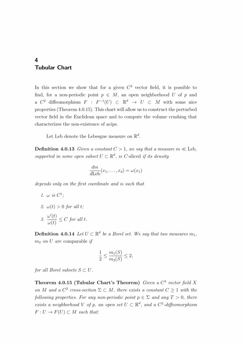
4Tubular Chart
In this section we show that for a given C3 vector field, it is possible to
find, for a non-periodic point p ∈ M , an open neighborhood U of p and
a C2 diffeomorphism F : F−1(U) ⊂ Rd → U ⊂ M with some nice
properties (Theorem 4.0.15). This chart will allow us to construct the perturbed
vector field in the Euclidean space and to compute the volume crushing that
characterizes the non-existence of acips.
Let Leb denote the Lebesgue measure on Rd.
Definition 4.0.13 Given a constant C > 1, we say that a measure m� Leb,
supported in some open subset U ⊂ Rd, is C-sliced if its density
dm
dLeb(x1, . . . , xd) = ω(x1)
depends only on the first coordinate and is such that
1. ω is C1;
2. ω(t) > 0 for all t;
3.ω′(t)
ω(t)≤ C for all t.
Definition 4.0.14 Let U ⊂ Rd be a Borel set. We say that two measures m1,
m2 on U are comparable if
1
2≤ m1(S)
m2(S)≤ 2,
for all Borel subsets S ⊂ U .
Theorem 4.0.15 (Tubular Chart’s Theorem) Given a C3 vector field X
on M and a C2 cross-section Σ ⊂ M , there exists a constant C ≥ 1 with the
following properties. For any non-periodic point p ∈ Σ and any T > 0, there
exists a neighborhood V of p, an open set U ⊂ Rd, and a C2-diffeomorphism
F : U → F (U) ⊂M such that:
Chapter 4. Tubular Chart 40
1. ϕt(V ) ⊂ F (U) for all t ∈ [−1, T + 1];
2. ϕt(p) = F (t, 0, . . . , 0), for all t ∈ [−1, T + 1];
3. the vector field X is tangent to the submanifold F ((Rd−1 × {0}) ∩ U);
4. F−1(Σ ∩ V ) ⊂ {0} × Rd−1;
5. NC(D(F−1(q)|TqΣ
)≤ C, for all q ∈ Σ ∩ V ;
6. ‖DF (z)‖ ≤ C, for all z ∈ U ;
7. ‖DF (z)ed‖·‖DF−1(F (z))‖ ≤ C, for all z ∈ U (where ed = (0, . . . , 0, 1) ∈Rd);
8. ‖D2F (z)( · , ed)‖ · ‖DF−1(F (z))‖ ≤ C, for all z ∈ U ;
9. if m is the Riemannian volume on M then (F−1)∗(m|F (U)) is comparable
to a C-sliced measure m on U ;
10. letting {P tp} (resp. {P t
0}) be the linear Poincare flow with base-point p
(resp. 0) for the vector field X on M (resp. X ≡ (F−1)∗X on U), we
have ‖P t,sp ‖ = ‖P t,s
0 ‖ for all t, s ∈ [0, T ].
In order to clarify the significance of this result, we comment informally
how it fits in our general strategy:
– The purpose of the Theorem 4.0.15 is to put the vector field on a
neighborhood of a segment of orbit in a kind of standard form in order
to make it easier to find perturbations with a (local) crushing property.
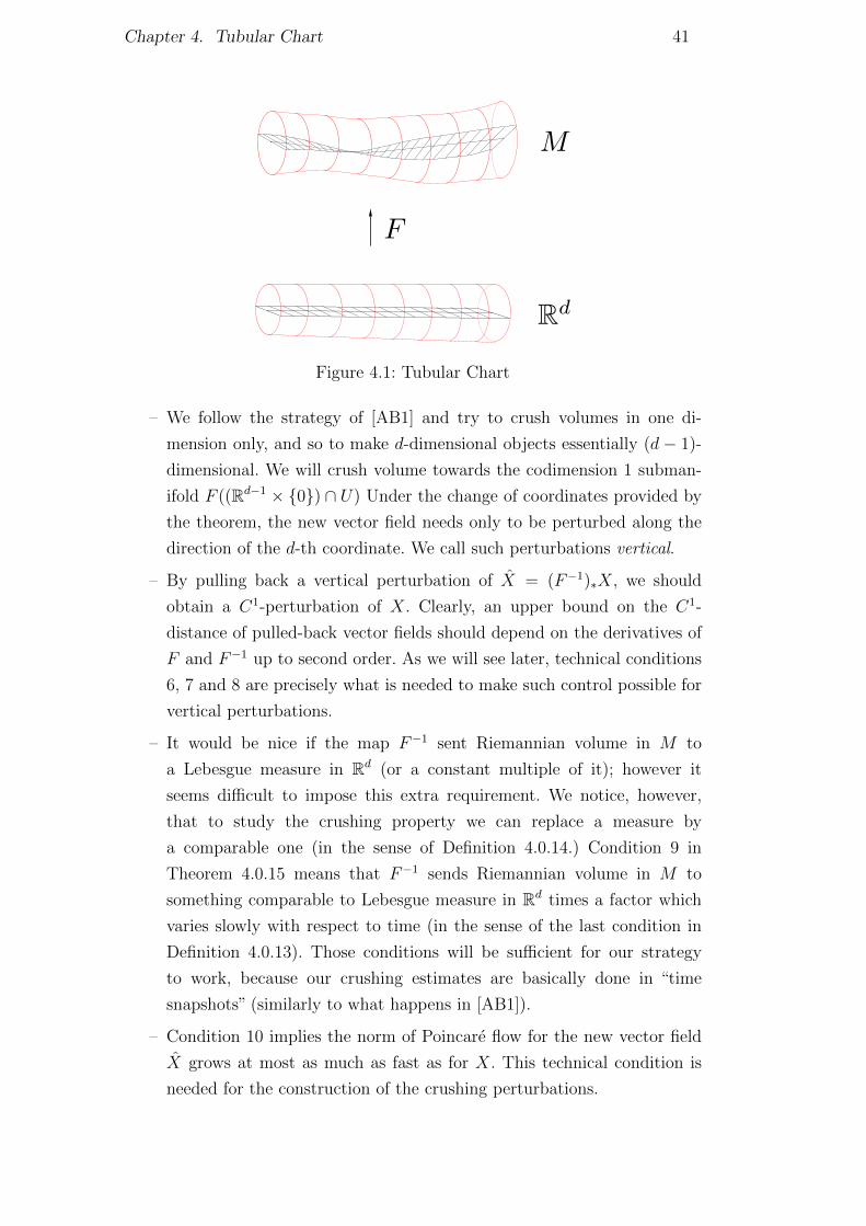
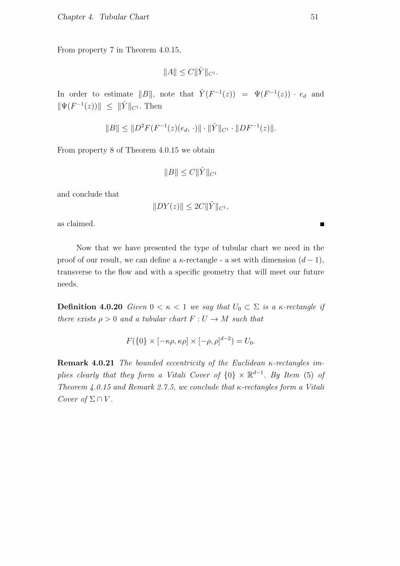
– Conditions 2, 3 and 4 mean that the chart “straightens” respectively a
segment of trajectory, a codimension 1 invariant submanifold containing
this trajectory, and the disk Σ; see Figure 4.1.
– The change of coordinates should be uniformly controlled in several ways;
this is expressed by a single control parameter C. If C were allowed to
depend on the time length T , the result would be much easier; indeed,
in that case one could take a change of coordinates with stronger and
simpler properties. However, it is essential to our strategy that C does
not depend on T .
– The diffeomorphism F can be highly non-conformal. (In fact, we will
see in the proof that the expansion rates along hyperplanes {t} × Rd−1
can be much smaller than along the line R × {0}d−1.) Nevertheless, its
restriction to Σ ∩ V is approximately conformal, as stated in condition
5.
Chapter 4. Tubular Chart 41
Figure 4.1: Tubular Chart
– We follow the strategy of [AB1] and try to crush volumes in one di-
mension only, and so to make d-dimensional objects essentially (d − 1)-
dimensional. We will crush volume towards the codimension 1 subman-
ifold F ((Rd−1 × {0}) ∩ U) Under the change of coordinates provided by
the theorem, the new vector field needs only to be perturbed along the
direction of the d-th coordinate. We call such perturbations vertical.
– By pulling back a vertical perturbation of X = (F−1)∗X, we should
obtain a C1-perturbation of X. Clearly, an upper bound on the C1-
distance of pulled-back vector fields should depend on the derivatives of
F and F−1 up to second order. As we will see later, technical conditions
6, 7 and 8 are precisely what is needed to make such control possible for
vertical perturbations.
– It would be nice if the map F−1 sent Riemannian volume in M to
a Lebesgue measure in Rd (or a constant multiple of it); however it
seems difficult to impose this extra requirement. We notice, however,
that to study the crushing property we can replace a measure by
a comparable one (in the sense of Definition 4.0.14.) Condition 9 in
Theorem 4.0.15 means that F−1 sends Riemannian volume in M to
something comparable to Lebesgue measure in Rd times a factor which
varies slowly with respect to time (in the sense of the last condition in
Definition 4.0.13). Those conditions will be sufficient for our strategy
to work, because our crushing estimates are basically done in “time
snapshots” (similarly to what happens in [AB1]).
– Condition 10 implies the norm of Poincare flow for the new vector field
X grows at most as much as fast as for X. This technical condition is
needed for the construction of the crushing perturbations.
Chapter 4. Tubular Chart 42
– The construction of the chart F uses the orthonormal frame flow (see
§ 2.4), whose class of differentiability is one less than the flow on M .
Since we need F to be C2, we ask X to be C3. And it is of course
necessary to ask Σ to be C2, in view of condition 4.
After those remarks, let us now prove Theorem 4.0.15:
Proof: By the Whitney embedding theorem, we can assume that M is
embedded in RN , for some large N > d. Moreover, by the Nash Embedding
Theorem, we can assume that the Riemannian metric on M is inherited from
the Euclidean metric on RN . (One could avoid appealing to Nash’s theorem by
noticing that, since M is compact, a change of Riemannian metric is absorbed
by a change of the constants in the statement of Theorem 4.0.15. Alternatively,
since our main theorem does not depend on the choice of the Riemannian
metric, we could have fixed a priori any suitable Riemannian metric to work
with.)
Fix a normal tubular neighborhood M ε ⊂ RN of M of some width
ε > 0, and the associate bundle projection π : M ε → M ; more precisely,
M ε = {z ∈ RN : d(z,M) ≤ ε}, and for each z ∈ M ε, π(z) is the point in M
which is closest to z.
Fix X ∈ X3(M). For any point p ∈ M and any orthonormal frame
f = (v1, . . . , vd) at TpM , we will define a mapGp,f : R×Bε →M , where Bε is the
closed ball in Rd−1 of center 0 and radius ε, as follows. Let {(v1(t), . . . , vd(t))}t∈Rbe the trajectory of the orthonormal frame flow induced by X (recall § 2.4),
with initial conditions
vi(0) = vi, 1 ≤ i ≤ d.
Then we define
Gp,f : R×Bε → M
(x1, x2, . . . , xd) 7→ π(ϕx1(p) +
∑dj=2 xjvj(x1)
)Since the orthonormal frame flow is C2 (because X is C3), this map is C2.
Moreover, by compactness of the orthonormal frame bundle, we can find a
constant C0 such that
‖DGp,f(z)‖ ≤ C0, ‖D2Gp,f(z)‖ ≤ C0, (4.1)
for all p ∈ Σ, all orthonormal frames f ∈ Fp, and all z ∈ R×Bε.
Now assume that p ∈ M is nonsingular (i.e., X(p) 6= 0) and f ∈ Fp
satisfiesf = (v1, . . . , vd) where v1 =
X(p)
‖X(p)‖. (4.2)
Chapter 4. Tubular Chart 43
Since G(x1, 0, . . . , 0) = ϕx1(p) ∈ M , and π is a C∞ retraction onto M , the
partial derivatives of Gp,f at (x1, 0 . . . , 0) are given by:
DGp,f(x1, 0, . . . , 0) · ej =
X(ϕx1(p)) = ‖X(ϕx1(p))‖v1(x1) if j = 1,
vj(x1) if j ≥ 2,(4.3)
where (e1, . . . , ed) is the canonical basis of Rd. In particular, the map Gp,f
is a local diffeomorphism at each point in the line R × {0}d−1 (under the
assumptions X(p) 6= 0 and (4.2)).
Next, fix a C2 cross-section Σ ⊂ M . Notice that the pairs (p, f) where
p ∈ Σ and f ∈ Fp satisfies (4.2) form a compact set. Since Σ is C2 and transverse
to X, for each such p and f, there is a neighborhood Vp of p such that
G−1p,f (Σ ∩ Vp) =
{(x, u) ∈ R× Rd−1 : x = gp,f(u)
}, (4.4)
where gp,f is a C2 function on a open neighborhood of 0 in Rd−1. By compact-
ness, there is a constant C1 such that
‖Dgp,f(0)‖ ≤ C1, ‖D2gp,f(0)‖ ≤ C1, (4.5)
for all p ∈ Σ and f satisfying (4.2). Also notice that gp,f(0) = 0.
Now fix p ∈ Σ and T > 0. The constant C that appears in the statement
of the Theorem will be exhibited later, but it will not depend on p and T .
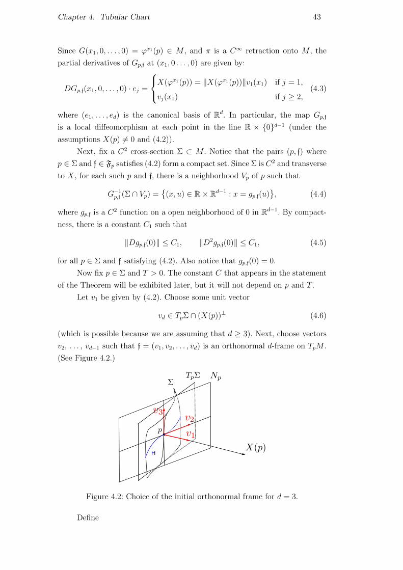
Let v1 be given by (4.2). Choose some unit vector
vd ∈ TpΣ ∩ (X(p))⊥ (4.6)
(which is possible because we are assuming that d ≥ 3). Next, choose vectors
v2, . . . , vd−1 such that f = (v1, v2, . . . , vd) is an orthonormal d-frame on TpM .
(See Figure 4.2.)
H
Figure 4.2: Choice of the initial orthonormal frame for d = 3.
Define
Chapter 4. Tubular Chart 44
α ≡ mint∈[−2,T+2]
‖X(ϕt(p))‖ . (4.7)
For simplicity of notation, let G = Gp,f and g = gp,f. Define the following linear
isomorphism
Lα : Rd → Rd
(x1, x2, . . . , xd) 7→ (x1, αx2, . . . , αxd)
Let
F1 = G ◦ Lα .
So (4.3) gives
DF1(x1, 0, . . . , 0) =
‖X(ϕx1(p))‖
α. . .
α
, (4.8)
where the matrix is relative to the bases (e1, . . . , ed) in Rd and
(v1(x1), . . . , vd(x1)) in Tϕx1 (p)M . By the inverse function theorem, there exists
a neighborhood U1 of [−2, T + 2]×{0}d−1 such that F1|U1 is a diffeomorphism
onto an open subset of M .
Notice that F1 already satisfies property 2, that is, F1(t, 0, . . . , 0) = ϕt(p).
The role of F4 is basically to straighten two codimension 1 submanifolds in
order to obtain properties 3 and 4.
We split Rd as R× Rd−2 × R and take coordinates (x,w, y) with x ∈ R,
w ∈ Rd−2, y ∈ R.
If follows from (4.4) that for a sufficiently small neighborhood V 3 p,
F−11 (Σ ∩ V ) =
{(x,w, y) ∈ R× Rd−1 : x = g(αw, αy)
}. (4.9)
Recalling the choice (4.7) of vd, we obtain:
∂g
∂y(0, 0) = Dg(0, 0) · ed = 0 . (4.10)
Define a diffeomorphism on a neighborhood of [−2, T +2]×dom(g) ⊂ Rd
by
F2(x,w, y) =(x− g(αw, αy), w, y
).
So F2 ◦F−11 (Σ∩ V ) ⊂ {0}×Rd−2×R. Let {ϕt} be the flow of the vector field
(F2 ◦ F−11 )∗X. Let H be a small neighborhood of 0 in {0} ×Rd−2 × {0}. Then
H ≡⋃
t∈[−1,T+1]
ϕt(H)
Chapter 4. Tubular Chart 45
is a codimension 1 submanifold of Rd containing the line [−1, T +1]×{0}d−2×{0}.
Claim 4.0.16 The tangent space of H at any point of this line is R×Rd−2×{0}.
Proof of the Claim: It follows from the definition of the orthonormal frame
flow that
Dϕt(p) · span(v1, . . . , vd−1) = span(v1(t), . . . , vd−1(t)).
Notice that the image of this space under D(F2 ◦ F−11 )(ϕt(p)) is exactly the
tangent space of H at (t, 0, 0). The claim follows.
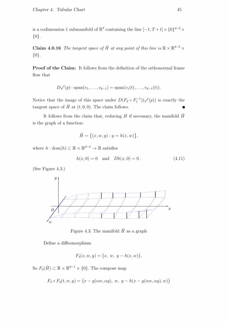
It follows from the claim that, reducing H if necessary, the manifold H
is the graph of a function:
H ={
(x,w, y) : y = h(x,w)},
where h : dom(h) ⊂ R× Rd−2 → R satisfies
h(x, 0) = 0 and Dh(x, 0) = 0 . (4.11)
(See Figure 4.3.)
Figure 4.3: The manifold H as a graph
Define a diffeomorphism
F3(x,w, y) =(x, w, y − h(x,w)
).
So F3(H) ⊂ R× Rd−1 × {0}. The compose map
F3 ◦ F2(t, w, y) =(x− g(αw, αy), w, y − h(x− g(αw, αy), w)
)
Chapter 4. Tubular Chart 46
is a diffeomorphism; let F2 = (F3 ◦ F2)−1, i.e.,
F4(x,w, y) =(x+ g(αw, αy + αh(x,w)), w, y + h(x,w)
).
Let us check that F = F1 ◦ F4 satisfies all properties in the statement of
the Theorem.
We have already mentioned that F1 satisfies property 2. Since F4 fixes
R× {0}d−1, the map F will clearly inherit this property.
Properties 4 and 3 are straightforward.
It follows from Property 4, that
DF−1(q)|TqΣ = (DF (F−1(q)))−1|{0}×Rd−1 . (4.12)
Thus, in order to check Property 5, observe that DF (0) · ej = αvj for
j = 2, . . . , d. In particular, DF (0) is conformal. Taking C ≥ 2, Property 5
follows by taking a sufficiently small neighborhood V = F−1(V ) of zero.
Using (4.11) and (4.10), we see that the derivative of F4 on the points in
R× {0}d−2 × {0} has the following (block) matrix expression:
DF4(t, 0, 0) =
1 α ∂g∂w
(0, 0) 0
0 idd−2 0
0 0 1
. (4.13)
In particular, using (4.5) and the fact that α ≤ ‖X‖C0 , we obtain
‖(DF4(x, 0, 0))±1‖ ≤ C2, (4.14)
where C2 depends only on X and Σ. Thus, reducing U if necessary, we can
assume that‖(DF4(z))±1‖ ≤ 2C2 for all z ∈ U. (4.15)
It follows from (4.7) and (4.8) that ‖DF1(x, 0, 0)‖ ≤ ‖X‖C0 . Reducing U if
necessary, we can assume that
‖DF1‖ ≤ 2‖X‖C0 on F4(U). (4.16)
Since F = F1 ◦F4, it follows from (4.15) and (4.16) that property 6 is satisfied,
provided the constant C is chosen bigger that 4C2‖X‖C0 .
Using (4.8) and (4.13), we have
DF (x, 0, 0)ed = DF1(F4(x, 0, 0)) ·DF4(x, 0, 0)ed
= DF1(x, 0, 0)ed = αvd(x).
Chapter 4. Tubular Chart 47
Reducing U , we obtain
‖DF (z)ed‖ ≤ 2α for all z ∈ U . (4.17)
It follows from (4.7) and (4.8) that ‖DF−11 (ϕx(p))‖ = α−1. So, using
(4.14), we have
‖DF−1(ϕx(p))‖ ≤ C2α−1,
for all x ∈ [0, T ]. Reducing U , if necessary, we obtain
‖DF−1(F (z))‖ ≤ 2C2α−1, for all z ∈ U . (4.18)
Putting this together with (4.17), we obtain
‖DF (z)ed‖ · ‖DF−1(F (z))‖ ≤ 4C2 ;
that is, property 7 is verified, provided we choose C ≥ 4C2.
Let us check property 8. First observe that the linear map D2F (z)(ed, ·)is the derivative of the map
z = (x,w, y) 7→ DF (z) · ed= DG(Lα ◦ F4(z)) ◦ Lα ◦DF4(z) · ed
= DG(Lα ◦ F4(z)) ·(α∂g
∂y(w, y) · e1 + α · ed
)= αΨ(z),
where we define Ψ as
Ψ(x,w, y) = DG(Lα ◦ F4(z)) ·(∂g
∂y(w, y) · e1 + ed
)Using (4.1), (4.15), (4.5), and that α ≤ ‖X‖C0 , we see that ‖DΨ‖ ≤ C3, for
some constant C3 depending only on X and Σ. That is, ‖D2F (z)(ed, ·)‖ ≤ C3α.
Putting this together with (4.18), we conclude that property 8 is satisfied,
provided C ≥ 2C2C3.
Let us check Property 9. For that matter, consider the measure m defined
by
m(S) =
∫S
αd−1‖X(ϕt(p))‖dtdx2 . . . dxd,
where S ⊂ U is a Borel set in Rd.
Notice that we can represent DF1 as a matrix that sends the orthonormal
base {e1, ed, . . . , ed} of Rd to the orthonormal base {v1(t), v2(t), . . . , vd(t)} of
Tϕt(p)M . Thus the Jacobian of F1 is the determinant of such matrix. Using
Chapter 4. Tubular Chart 48
(4.8) and (4.13), we see that the Jacobian of F along (t, 0, . . . , 0) is
Jac(F )(t, 0, . . . , 0) = αd−1‖X(ϕt(p))‖.
Therefore, we can reduce U if necessary, to obtain
1
2≤ Jac(F )(z)
αd−1‖X(ϕt(p))‖≤ 2, (4.19)
for all z ∈ U .
By the change of variables formula,
F−1∗ (m)(S) = m(F (S)) =
∫S
Jac(F )(t, x1, . . . , xd)dtdx2 . . . dxd,
which together with (4.19) leads us to conclude that m is comparable to
F−1∗ (m)|F (U). In order to show that m is a C-sliced measure, observe that
if ω(t) = αd−1‖X(ϕt(p))‖, then
ω′(t) ≤ αd−1
∥∥∥∥dX(ϕt(p))
dt
∥∥∥∥≤ αd−1‖DX(ϕt(p)) ·X(ϕt(p))‖
≤ αd−1‖DX‖C0 · ‖X(ϕt(p))‖
≤ Cω(t),
provided that the constant C is chosen bigger then the C1-norm of X.
It only remains to check Property 10. For that end, consider the canonical
basis in Rd and the basis (v1(t), . . . , vd(t)) at the tangent space of M at ϕt(p).
We can express linear maps as matrices according to those bases. Thus:
Dϕs(t, 0, 0) = (DF (t+ s, 0, 0))−1 ◦Dϕs(ϕtp) ◦DF (t, 0, 0)
=
(‖X(ϕt+sp)‖−1 ∗
0 α−1id
)(‖X(ϕt+sp)‖‖X(ϕtp)‖ ∗
0 P t,sp
)(‖X(ϕtp)‖ ∗
0 αid
)
=
(1 ∗0 P t,s
p
).
So the matrices of P t,s0 and P t,s
p coincide. Since we are taking matrices with
respect to orthonormal bases, Property 10 is satisfied.
Remark 4.0.17 Notice that Theorem 4.0.15 provides no uniform estimate
for the C1 norm of the new vector field X = (F−1)∗X. It neither provides an
Chapter 4. Tubular Chart 49
estimate for the C2 norm of F (and in fact, ‖F‖C2 can be arbitrarily large, as
shown by Example 4.0.18 below). However, no such estimates will be necessary.
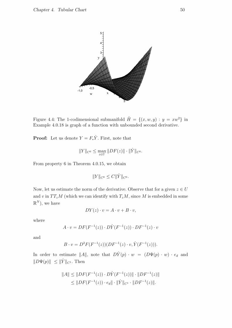
Example 4.0.18 Let us exhibit one example where ‖F‖C2 can be arbitrarily
large. The example will be constructed in M = R3, but it is easy to adapt the
construction to a compact manifold M of dimension d = 3. For (x,w, y) ∈ R3,
define X(x,w, y) = (1, 0, w2). The flow induced by X is given by
ϕt(x0, w0, y0) = (x0 + t, w0, y0 + w20t).
If p = (0, 0, 0), Property 2 is already satisfied and, in particular, for any T > 0
we have α = 1. Suppose Σ is a disc in R × {0} × R. By (4.2) we have
v1 = (1, 0, 0); suppose we choose v2 = (0, 1, 0), v3 = (0, 0, 1). Then the frame
(v1(t), v2(t), v3(t)) does not depend on t and H is the graph of h(x,w) = xw2
(See Figure 4.4). Since we are already placed in R3 and in a context where
the cross-section Σ and the base orbit are already “straight”, the role of the
diffeomorphism F is to straighten H, that is
F (x,w, y) = F4(x,w, y) = (x,w, y + h(x,w)).
Observe that the curvature of the surface H along the x-axis tends to infinity.
In fact,
‖D2F (x, 0, 0)‖ ≥∣∣∣∣∂2h(x, 0)
∂w2
∣∣∣∣ = 2|x|.
Therefore, the second derivative of F is unbounded.
Let F : U ⊂ Rd → F (U) ⊂M be given by Theorem 4.0.15. As explained
above, we need to compare the C1 norm of a vector field Y ∈ X1(U) and its
push-forward F∗Y ∈ X1(F (U)). Actually we will only study this problem for
vertical vector fields Y ; the norm comparison is then given by the following:
Proposition 4.0.19 Let X ∈ X3(M) and F : U ⊂ Rd → F (U) ⊂M be given
by Theorem 4.0.15. If Ψ : Rd → R is a C1 map and Y ∈ X1(U) is a vector
field of the form
(x1, x2, . . . , xd)→ (0,Ψ(x1, x2, . . . , xd), 0, . . . , 0),
then
‖F∗Y ‖C1 ≤ 2C‖Y ‖C1 ,
where C > 1 is the constant given by Theorem 4.0.15.
Chapter 4. Tubular Chart 50
1,00,5
0,000
w
-0,5
1
2
1
-1,0
y3
4
2
5
x 34
5
Figure 4.4: The 1-codimensional submanifold H = {(x,w, y) : y = xw2} inExample 4.0.18 is graph of a function with unbounded second derivative.
Proof: Let us denote Y = F∗Y . First, note that
‖Y ‖C0 ≤ maxz∈U‖DF (z)‖ · ‖Y ‖C0 .
From property 6 in Theorem 4.0.15, we obtain
‖Y ‖C0 ≤ C‖Y ‖C0 .
Now, let us estimate the norm of the derivative. Observe that for a given z ∈ Uand v in TTzM (which we can identify with TzM , since M is embedded in some
RN), we have
DY (z) · v = A · v +B · v,
where
A · v = DF (F−1(z)) ·DY (F−1(z)) ·DF−1(z) · v
and
B · v = D2F (F−1(z))(DF−1(z) · v, Y (F−1(z))).
In order to estimate ‖A‖, note that DY (p) · w = (DΨ(p) · w) · ed and
‖DΨ(p)‖ ≤ ‖Y ‖C1 . Then
‖A‖ ≤ ‖DF (F−1(z)) ·DY (F−1(z))‖ · ‖DF−1(z)‖
≤ ‖DF (F−1(z)) · ed‖ · ‖Y ‖C1 · ‖DF−1(z)‖.
Chapter 4. Tubular Chart 51
From property 7 in Theorem 4.0.15,
‖A‖ ≤ C‖Y ‖C1 .
In order to estimate ‖B‖, note that Y (F−1(z)) = Ψ(F−1(z)) · ed and
‖Ψ(F−1(z))‖ ≤ ‖Y ‖C1 . Then
‖B‖ ≤ ‖D2F (F−1(z)(ed, ·)‖ · ‖Y ‖C1 · ‖DF−1(z)‖.
From property 8 of Theorem 4.0.15 we obtain
‖B‖ ≤ C‖Y ‖C1
and conclude that
‖DY (z)‖ ≤ 2C‖Y ‖C1 ,
as claimed.
Now that we have presented the type of tubular chart we need in the
proof of our result, we can define a κ-rectangle - a set with dimension (d− 1),
transverse to the flow and with a specific geometry that will meet our future
needs.
Definition 4.0.20 Given 0 < κ < 1 we say that U0 ⊂ Σ is a κ-rectangle if
there exists ρ > 0 and a tubular chart F : U →M such that
F ({0} × [−κρ, κρ]× [−ρ, ρ]d−2) = U0.
Remark 4.0.21 The bounded eccentricity of the Euclidean κ-rectangles im-
plies clearly that they form a Vitali Cover of {0} × Rd−1. By Item (5) of
Theorem 4.0.15 and Remark 2.7.5, we conclude that κ-rectangles form a Vitali
Cover of Σ ∩ V .
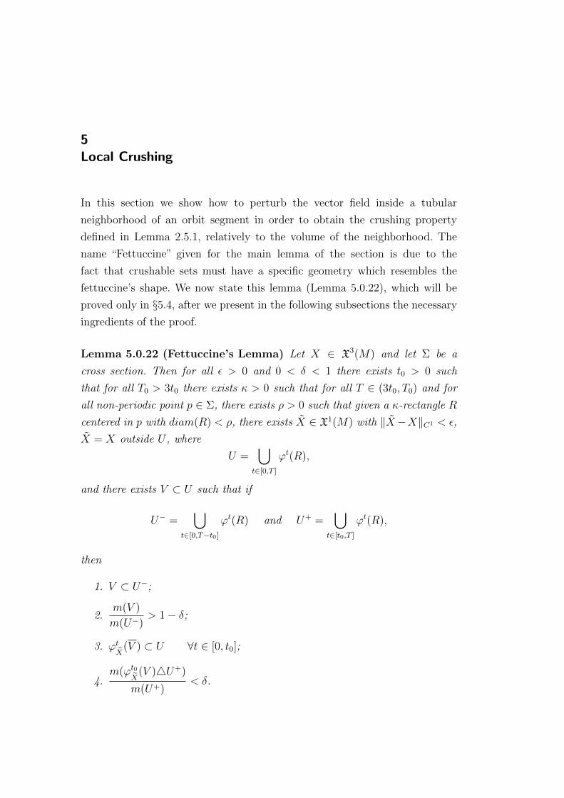
5Local Crushing
In this section we show how to perturb the vector field inside a tubular
neighborhood of an orbit segment in order to obtain the crushing property
defined in Lemma 2.5.1, relatively to the volume of the neighborhood. The
name “Fettuccine” given for the main lemma of the section is due to the
fact that crushable sets must have a specific geometry which resembles the
fettuccine’s shape. We now state this lemma (Lemma 5.0.22), which will be
proved only in §5.4, after we present in the following subsections the necessary
ingredients of the proof.
Lemma 5.0.22 (Fettuccine’s Lemma) Let X ∈ X3(M) and let Σ be a
cross section. Then for all ε > 0 and 0 < δ < 1 there exists t0 > 0 such
that for all T0 > 3t0 there exists κ > 0 such that for all T ∈ (3t0, T0) and for
all non-periodic point p ∈ Σ, there exists ρ > 0 such that given a κ-rectangle R
centered in p with diam(R) < ρ, there exists X ∈ X1(M) with ‖X−X‖C1 < ε,
X = X outside U , where
U =⋃
t∈[0,T ]
ϕt(R),
and there exists V ⊂ U such that if
U− =⋃
t∈[0,T−t0]
ϕt(R) and U+ =⋃
t∈[t0,T ]
ϕt(R),
then
1. V ⊂ U−;
2.m(V )
m(U−)> 1− δ;
3. ϕtX
(V ) ⊂ U ∀t ∈ [0, t0];
4.m(ϕt0
X(V )4U+)
m(U+)< δ.
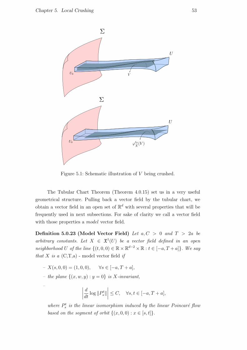
Chapter 5. Local Crushing 53
Figure 5.1: Schematic illustration of V being crushed.
The Tubular Chart Theorem (Theorem 4.0.15) set us in a very useful
geometrical structure. Pulling back a vector field by the tubular chart, we
obtain a vector field in an open set of Rd with several properties that will be
frequently used in next subsections. For sake of clarity we call a vector field
with those properties a model vector field.
Definition 5.0.23 (Model Vector Field) Let a, C > 0 and T > 2a be
arbitrary constants. Let X ∈ X1(U) be a vector field defined in an open
neighborhood U of the line {(t, 0, 0) ∈ R×Rd−2×R : t ∈ [−a, T + a]}. We say
that X is a (C,T,a) - model vector field if
– X(s, 0, 0) = (1, 0, 0), ∀s ∈ [−a, T + a],
– the plane {(x,w, y) : y = 0} is X-invariant,
– ∣∣∣∣ ddt log ‖P ts‖∣∣∣∣ ≤ C, ∀s, t ∈ [−a, T + a],
where P ts is the linear isomorphism induced by the linear Poincare flow
based on the segment of orbit {(x, 0, 0) : x ∈ [s, t]}.
Chapter 5. Local Crushing 54
Depending on the context, some of the constants C, T and a may be
omitted from the notation of model vector fields. Possibly for they are implicitly
understood, possibly for being unnecessary in some computation.
5.1Crushing-Time
Once we have constructed a chart which permits us to work with model vector
fields, next step will be defining the crushing-perturbation of a general model
vector field. The main idea is to add small vertical vectors to the original vector
field, bringing trajectories closer to the invariant plane and, consequently,
crushing volume in that direction (See Figure 5.2). Since these new vertical
components need to be very small, in order to obtain a significant “vertical
deviation” of the original trajectories, a long period of time must elapse. This
amount of time will be called crushing-time and its precise definition is given
by Lemma 5.1.2.
Let πd : R× Rd−2 × R the standard projection in the d-th coordinate.
Then Dπd(x,w, y)X(x,w, y) is simply the d-th coordinate of the vector
X(x,w, y). Define α : R× Rd−2 by
α(x,w) = D(πd ◦X)(x,w, 0) · ed.
Since X is C1 we can write
Dπd(x,w, y)X(x,w, y) = α(x,w)y + r(x,w, y), (5.1)
where r : Rd −→ R is a continuous function satisfying
limy→0
r(x,w, y)
y= 0. (5.2)
Proposition 5.1.1 For all ε′ > 0 and T2 > T1 > 0 there exist ρ > 0 and such
that if max{‖w‖, |y|} < ρ and x ∈ [0, T1] then
‖ϕt(x,w, y)− (x+ t, 0, 0)‖ < ε′,
for all t ∈ [0, T2 − T1], where ϕt is the flow generated by the vector field X.
Proof: This is an immediate consequence of the continuity of the flow and
the first property of model vector fields.
Lemma 5.1.2 Let ε > 0 and 0 < δ < 1 be given. Then for any
T > t0 ≡ 3− 2 log(δ)
ε,
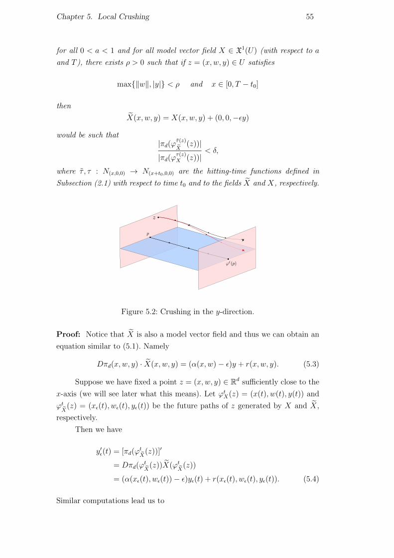
Chapter 5. Local Crushing 55
for all 0 < a < 1 and for all model vector field X ∈ X1(U) (with respect to a
and T ), there exists ρ > 0 such that if z = (x,w, y) ∈ U satisfies
max{‖w‖, |y|} < ρ and x ∈ [0, T − t0]
then
X(x,w, y) = X(x,w, y) + (0, 0,−εy)
would be such that|πd(ϕτ(z)
X(z))|
|πd(ϕτ(z)X (z))|
< δ,
where τ , τ : N(x,0,0) → N(x+t0,0,0) are the hitting-time functions defined in
Subsection (2.1) with respect to time t0 and to the fields X and X, respectively.
Figure 5.2: Crushing in the y-direction.
Proof: Notice that X is also a model vector field and thus we can obtain an
equation similar to (5.1). Namely
Dπd(x,w, y) · X(x,w, y) = (α(x,w)− ε)y + r(x,w, y). (5.3)
Suppose we have fixed a point z = (x,w, y) ∈ Rd sufficiently close to the
x-axis (we will see later what this means). Let ϕtX(z) = (x(t), w(t), y(t)) and
ϕtX
(z) = (xε(t), wε(t), yε(t)) be the future paths of z generated by X and X,
respectively.
Then we have
y′ε(t) = [πd(ϕtX
(z))]′
= Dπd(ϕtX
(z))X(ϕtX
(z))
= (α(xε(t), wε(t))− ε)yε(t) + r(xε(t), wε(t), yε(t)). (5.4)
Similar computations lead us to
Chapter 5. Local Crushing 56
y′(t) = α(x(t), w(t))y(t) + r(x(t), w(t), y(t)). (5.5)
Proposition (5.1.1) together with the continuity of function α permit us to take
ρ > 0 sufficiently small such that if max{‖w‖, |y|} < ρ and x ∈ [−a, T − t0]
then
|α(x(t), w(t))− ax(t)| < ε/8 and |α(xε(t), wε(t))− ax(t)| < ε/8,
for all t ∈ [0, t0], where ax(s) ≡ α(x+s, 0). Notice that the choice of ρ depends
on T but does not depend on x.
By equation (5.2) and by the compactness of V , we can reduce ρ, if
necessary, to guarantee that
|r(xε(t), wε(t), yε(t))| ≤ε|yε(t)|
8and |r(x(t), w(t), y(t))| ≤ ε|y(t)|
8,
for all t ∈ [0, t0] and for all (x,w) in the compact domain.
From these estimates and from equations (5.4) and (5.5) we can deduce
the following inequalities:
y′ε(t) ≤ (ax(t)− 7ε/8)yε(t) + r(xε(t), wε(t), yε(t)) ≤ (ax(t)− 3ε/4)yε(t) (5.6)
y′(t) ≥ (ax(t)− ε/8)y(t) + r(x(t), w(t), y(t)) ≥ (ax(t)− ε/4)y(t). (5.7)
Besides that, we want to consider ρ > 0 small enough (as in Remark
2.1.6) to obtain
|τ(z)− t0| < min{a
2,ε
4M
}and |τ(z)− t0| < min
{a2,ε
4M
},
where
M = sups∈[−a,T+a]
|α(s, 0)|.
Chapter 5. Local Crushing 57
Once we have all these estimates, we can conclude that
yε(τ(z))
y(τ(z))≤yε(0) exp(−3ετ(z)/4) exp
(∫ τ(z)
0ax(t)dt
)y(0) exp(−ετ(z)/4) exp
(∫ τ(z)
0ax(t)dt
)
≤ exp(−3ε(t0 − 1)/4 + ε(t0 + 1)/4) exp
(|τ(z)− τ(z)| sup
t∈[0,t0+1]
|ax(t)|
)
≤ exp
((2− t0)ε
2
)exp
( ε
2MM)
= exp(log(δ)) = δ.
5.2Sliced Tube
In this Subsection, besides introducing some useful new notation, we will state
and prove Proposition 5.1.1, that will allow us to work with more convenient
sets - the sliced tubes, instead of the standard tubular neighborhoods.
We say that B ⊂ Rd is a ball if it is a convex compact set, symmetric
about the origin.
Definition 5.2.1 (K-Ball) Let B(0, r) denote the Euclidean ball with radius
r. Given K > 1 we say that a ball B is a K-ball if
B(0, K−1) ⊂ B ⊂ B(0, K).
Remark 5.2.2 Let K > 1 and let B ⊂ Rd be a K-ball. Then there exists a
norm ‖ · ‖B such that
1. B = {v ∈ Rd : ‖v‖B ≤ 1};
2. K−1‖v‖ ≤ ‖v‖B ≤ K‖v‖ ∀v ∈ Rd.
Remark 5.2.3 Notice that, since the cube B = [−1, 1]d is inscribed in a sphere
with radius√d/2 and circumscribed on a sphere with radius 1/2, the hypothesis
of Remark 5.2.2 is satisfied for any K > max{2,√d/2} and the conclusion, in
this case, holds with ‖ · ‖B being the norm of the maximum.
Chapter 5. Local Crushing 58
Remark 5.2.4 Let P t = P t0 be the family of linear isomorphisms induced by
the linear Poincare flow over the base-orbit of a (C, T,∆)-model vector field.
Notice that, by the sub-exponential growth of ‖P t‖ and Remark 5.2.3, we can
conclude that, for all t ∈ [0, T + ∆], P t([−1, 1]d−2) is a K-ball of Rd−2 with
K = max
{2,
√d− 2
2
}eC(T+∆).
Fix a model vector field X ∈ X1(U) and let P ts : Rd−1 → Rd−1 denote the
linear isomorphism induced by the linear Poincare flow on the segment [s, t]
of the orbit of zero (Definition 2.3.8). Define also βts ≡ |〈P ts(ed), ed〉|, where
ed = (0, 0, . . . , 0, 1). Given an interval I = [a, b] on the real line, κ ∈ (0, 1),
r > 0 and a ball B ⊂ Rd−2 we define a sliced tube SB(κ, r, I) by
SB(κ, r, I) ≡⋃s∈I
({s} × P sa (rB × {0})× [−κrβsa, κrβsa]) .
We most frequently deal with a special type of sliced tube, for which the ball
and the height of the slices depend on the left edge of I.
Definition 5.2.5 (Standard Sliced Tube) The standard sliced tube is de-
fined by
S(κ, r, I) ≡⋃s∈I
({s} × P s([−r, r]d−2 × {0})× [−κrβs, κrβs]
),
where P s = P s0 and βs = |〈P se2, e2〉|.
Remark 5.2.6 Notice that the standard sliced tube is a sliced tube with a
change of scale in direction y. In fact, by the cocycle property of the linear
Poincare flow, we can deduce that
S(κ, r, [a, b]) = SB(βaκ, r, [a, b]),
where B = P a([−1, 1]d−2 × {0}).
It is convenient to work with sliced tubes (instead of the usual tubular
neighborhood) because these sets are saturated by a family of cross sections
(the slices), each one being orthogonal to the base-orbit of the model vector
field. The fact that the slices of the tube are intrinsically related to the linear
Poincare flow is also an important feature of these sets, since it makes possible
the comparison between tubular neighborhoods and sliced tubes.
Chapter 5. Local Crushing 59
Proposition 5.2.7 (Approximation by sliced tubes) Given ∆ > 0, T >
2∆, C > 0, λ > 1 and K > 1, there exist κ0 ∈ (0, 1) and ρ0 > 0 such that,
for all (C, T,∆)-model vector field X, for any κ ∈ (0, κ0), ρ ∈ (0, ρ0), for all
interval I = [a, b] ⊂ [0, T ] satisfying |I| > 2∆ and for any K-ball B ⊂ Rd−2 we
have
SB(κ, ρλ−1, [a, b−∆]) ⊂⋃
t∈[0,b−a]
ϕt(Ua) ⊂ SB(κ, ρλ, [a, b+ ∆]),
where Ua = {a} × ρB × [−κρ, κρ].
Note that as ∆ > 0 approaches zero and as λ > 1 approaches 1, the
better the approximation becomes. On the other hand, in order to achieve a
good approximation of a tubular neighborhood by sliced tubes, we need to
impose that the initial slice (Ua) is sufficiently small (ρ � 1) and sufficiently
thin (κ� 1). Before proving Proposition 5.2.7, we state and prove a technical
lemma which shows the relation between κ and the distortion of the sliced tube
in the w-direction. This technical lemma is an adaptation of [AB1, Lemma 5]
to our context.
Lemma 5.2.8 (Approximation of the linear part) Given λ > 1, T > 0,
C > 0 and K > 1 there exists κ0 ∈ (0, 1) such that for any (C, T )-model vector
field X, any κ ∈ (0, κ0) and for any K-ball B ⊂ Rd−2 we have
(λ−1P ts(B×{0}))×[−βtκ, βtκ] ⊂ P t
s(B×[−κ, κ]) ⊂ (λP ts(B×{0}))×[−βtκ, βtκ],
for all [s, t] ∈ [0, T ].
Proof: In order to simplify notation, we will write P ts(B), instead of P t
s(B ×{0}).
By the invariance of the plane {y = 0}, we have, for all s, t ∈ [0, T ],
P ts(w, y) =
(Ats Bt
s
0 βts
)(w
y
).
And in this case,
(P ts)−1 = P s
t =
((Ats)
−1 −(βts)−1(Ats)
−1Bts
0 (βts)−1
)
Take
κ0 =λ− 1
KλMT
,
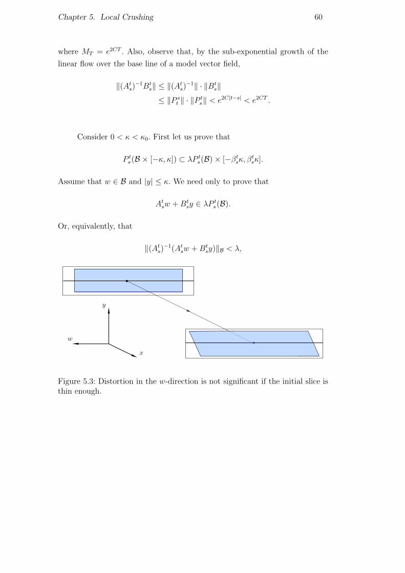
Chapter 5. Local Crushing 60
where MT = e2CT . Also, observe that, by the sub-exponential growth of the
linear flow over the base line of a model vector field,
‖(Ats)−1Bts‖ ≤ ‖(Ats)−1‖ · ‖Bt
s‖
≤ ‖P st ‖ · ‖P t
s‖ < e2C|t−s| < e2CT .
Consider 0 < κ < κ0. First let us prove that
P ts(B × [−κ, κ]) ⊂ λP t
s(B)× [−βtsκ, βtsκ].
Assume that w ∈ B and |y| ≤ κ. We need only to prove that
Atsw +Btsy ∈ λP t
s(B).
Or, equivalently, that
‖(Ats)−1(Atsw +Btsy)‖B < λ,
Figure 5.3: Distortion in the w-direction is not significant if the initial slice isthin enough.
Chapter 5. Local Crushing 61
Where ‖ · ‖B is the norm given by Remark 5.2.2. Indeed,
‖(Ats)−1(Atsw +Btsy)‖B = ‖w + (Ats)
−1Btsy‖B
≤ ‖w‖B + ‖(Ats)−1Btsy‖B
≤ 1 +K‖(Ats)−1Btsy‖
≤ 1 +K‖(Ats)−1Bts‖ · |y|
≤ 1 +K ·MTκ < λ,
as we wanted to show. On the other hand, assume that
(w, y) ∈ λ−1P ts(B)× [−βtsκ, βtsκ],
Let y be such that |y| ≤ κ and w ∈ B such that y = βtsy and w = λ−1Atsw.
Then we have that
(P ts)−1(w, y) = (λ−1w − (Ats)
−1Btsy, y),
So we need only to prove that
‖λ−1w − (Ats)−1Bt
sy‖B ≤ 1.
And indeed,
‖λ−1w − (Ats)−1Bt
sy‖B ≤ λ−1‖w‖B + ‖(Ats)−1Btsy‖B
≤ λ−1 +K‖(Ats)−1Btsy‖
≤ λ−1 +K ·MTκ ≤ 1.
Proof of Proposition 5.2.7:
Take any 1 < λ < λ and choose κ > 0 as in Lemma 5.2.8, such that
λ−1P sa (B × {0})× [−κβsa, κβsa] ⊂ P s
a (B × [−κ, κ])
⊂ λP sa (B × {0})× [−κβsa, κβsa], (5.8)
for all [a, s] ∈ [0, T ].

Chapter 5. Local Crushing 62
Let τs = τs−a,(a,0,0) be the hitting-time function (Definition 2.1.2) with
respect to the flow ϕ, with time s− a and base point (a, 0, 0).
Denote by Ns the subspace Nϕs((a,0,0)) ⊂ Tϕs((a,0,0))M orthogonal to
X(ϕs((a, 0, 0))) and let Φs : Ua → Ns be the Poincare Map with respect
to the flow ϕ and time s− a, that is
Φs(p) = ϕτs(p)(p).
Choose ρ > 0 small enough so that if p ∈ Ua = Ua(κ, ρ) then
|τs(p)− s| < ∆ for all s ∈ [a, T + ∆], and in particular,
τα−∆(p) < α < τα+∆(p) < τβ−∆(p) < β < τβ+∆,
for all a < α < β < T with β − α > 2∆. So⋃s∈[α+∆,β−∆]
Φs(Ua) ⊂⋃
s∈[α,β]
ϕs(Ua) ⊂⋃
s∈[α−∆,β+∆]
Φs(Ua). (5.9)
Figure 5.4: |τs(p)− s| < ∆ for all s ∈ [a, T + ∆].
Since
DΦs(a,0,0) = P s
a (See Proposition 2.3.9),
we can use the Taylor Formula to obtain
Φs(p) = Φs((a, 0, 0))︸ ︷︷ ︸(a+s,0,0)
+P sa (p) + r(p)

Chapter 5. Local Crushing 63
where r : U0 → Rd−1 satisfies
lim‖p‖→0
‖r(p)‖‖p‖
= 0.
Notice that if r is identically zero then the conclusion of the proposition follows
from (5.8) and (5.9). Taking a smaller ρ if necessary, the general case follows
from Taylor approximation.
Corollary 5.2.9 (Standard Approximation) Given ∆ > 0, T > 2∆,
C > 0 and λ > 1, there exist κ0 ∈ (0, 1) and ρ0 > 0 such that, for all
(C, T,∆)-model vector field X, for any κ ∈ (0, κ0), ρ ∈ (0, ρ0) and for all
interval I = [a, b] ⊂ [0, T ] satisfying |I| > 2∆ we have
S(κ, ρλ−1, I∆) ⊂⋃t∈I
ϕt(U0) ⊂ S(κ, ρλ, I∆),
where U0 = {0} × [−ρ, ρ]d−2 × [−κρ, κρ].
Proof: Recall that, by Remark 5.2.6,
S(κ, ρ, [a, b]) = SBa(βaκ, ρ, [a, b]),
where Ba = P a([−1, 1]d−2 × {0}). Let κ0 ∈ (0, 1) and ρ0 > 0 be given by
Proposition 5.1.1 for the K obtained by Remark 5.2.4. The Corollary follows
by taking
κ0 = κ0e−C(T+∆)
and by observing that βa < ‖P a0 ‖ < eC(T+∆).
Remark 5.2.10 Notice that if X is a C-model vector field with associated
linear Poincare flow given by
P ts =
(Ats Bt
s
0 βts
),
then the vector field given by
Xε(x,w, y) = X(x,w, y)− εy · ed
is a (C + ε)-model vector field with the associated linear Poincare flow given
by
P ts =
(Ats Bt
s
0 e−ε(t−s)βts
).
Chapter 5. Local Crushing 64
Proposition 5.2.11 (Perturbed sliced tube) Let X be model vector field,
ε > 0 and Xε be as in the previous Remark, that is, Xε(x,w, y) = X(x,w, y)−yε · ed. Then, for any κ ∈ (0, 1), r > 0 and any I = [a, b] ⊂ [0,∞), we have
1. πx(SB(κ, r, I)) = πx(SB(κ, r, I));
2. πw(SB(κ, r, I)) = πw(SB(κ, r, I));
3. πy(SB(κ, r, I)) ⊂ πy(SB(κ, r, I)),
where SB(κ, r, I) denotes de sliced tube with respect to Xε and πx, πw, πy are
the projections in directions x,w and y, respectively. In Particular,
SB(κ, r, I) ⊂ SB(κ, r, I).
Proof: The first conclusion is trivial, since the projection in the coordinate x
of a sliced tube is I. The second conclusion is a direct consequence of Remark
5.2.10, since
P ts |{y=0} = Ats = P t
s |{y=0}.
In order to see that third consequence is also true, notice that, by Re-
mark 5.2.10,
P ts |{w=0} = e−ε(t−s)βts < βts,
since we are considering 0 < s < t.
5.3Bump Function
In the previous subsection we saw that, in terms of volume, it is possible to
approximate a tubular neighborhood by two sliced tubes: one that contains the
neighborhood, and other that is contained in it. In this subsection, we show
how to construct a bump function with small C1 norm, supported on the inner
(standard) sliced tube.
Remark 5.3.1 Given a C-model vector field X, the function βt(x) =
|〈P tx(e2), e2〉|, defined inside a sliced tube with respect to X is a linear cocy-
cle in R over ϕtX . Moreover, its logarithmic derivative is bounded by C. In
other words, if we fix x ∈ R and let t vary, we have that∣∣∣∣βt(x)′
βt(x)
∣∣∣∣ ≤ C.
Proposition 5.3.2 (Bump Function) Given ε > 0 and 0 < γ < 1 there
exists 0 < ε′ < ε such that for all T0, a, C > 0 there exist 0 < κ0 < 1 and
Chapter 5. Local Crushing 65
r0 > 0 such that for all (C, T0, a)-model vector field X and for any T ∈ (2a, T0),
κ ∈ (0, κ0) and r ∈ (0, r0) there exists a function Ψ : Rd → R such that
1. Ψ = 0 outside S(κ, r, [−a, T + a]);
2. Ψ = ε′ on S(κ, r(1− γ), [a, T − a]);
3. ‖yΨ(x,w, y)‖C1 < ε, for all (x,w, y) ∈ Rd.
Proof: Let ε′ =εγ
2 + γand fix any C > 0, any large T0 > 0 and any small
a > 0. Define
κ0 = e−2C(T0+2a)
and take T ∈ (2a, T0), κ ∈ (0, κ0) and any (C, T0, a)-model vector field X.
Observe that, by the third property of model vector fields, by Remarks 2.6.1
and 5.3.1, we can conclude that
(βx‖(P x)−1‖)−1 < sup β−1x · sup ‖(P x)−1‖−1
= (inf βx)−1 · (inf ‖(P x)−1‖)−1
< e−2Cx < e−2C(T0+2a) = κ0.
Consider a bump-function ξ1 : R→ R such that:
– ξ1(x) = 0, if x ∈ R\[−1, 1];
– ξ1(x) = 1, if x ∈ [−1 + γ, 1− γ];
– |ξ′1(x)| ≤ 2γ, for all x ∈ R.
Also define another bump-function ξ2 : R→ R such that
– ξ2(x) = 0, if x ∈ R\[−a, T + a];
– ξ2(x) = 1, if x ∈ [a, T − a],
– |ξ′2(x)| ≤ 2a, for all x ∈ R.
For some r > 0 (we will estimate r a posteriori) we define the bump-
function
Ψ: R× R× Rd−2 → R(x,w, y) 7→ ε′ξ1(κ−1r−1β−1
x y)ξ1(r−1‖(P x)−1w‖)ξ2(x)
Chapter 5. Local Crushing 66
Properties 1 and 2 are very easy to check and we only need to estimate
the derivative of yΨ(x,w, y) inside the tube S(κ, r, [−a, T + a]). So in next
computations we can always assume that
|y| < κβxr (5.10)
and also that‖(P x)−1w‖ < r. (5.11)
In order to prove that
‖yΨ(x,w, y)‖C1 < ε,
we first observe that
|yΨ(x,w, y)| < |y|ε′ < ε.
Now let us compute the derivatives.
1. ∣∣∣∣ ∂∂y (yΨ(x,w, y))
∣∣∣∣ < |Ψ(x,w, y)|+ |y|∣∣∣∣ ∂∂y (Ψ(x,w, y))
∣∣∣∣< ε′ + |y|
(ε′
κrβx|ξ′1(κ−1r−1β−1
x y)| · |ξ1(r−1‖(P x)−1w‖)| · |ξ2(x)|)
< ε′(
1 +2
γ
)
<εγ
(γ + 2)
(γ + 2)
γ= ε;
2.
‖D3(yΨ(x,w, y))‖ < ε′|y|r|ξ′1(r−1‖(P x)−1w‖)| · ‖(P x)−1‖
< ε′κrβxr
2
γ‖(P x)−1‖
< ε′2
γκβx‖(P x)−1‖,
By the choice of κ0,
κβx‖(P x)−1‖ < 1
Chapter 5. Local Crushing 67
and we have:
‖D3(yΨ(x,w, y))‖ < ε′2
γ
<εγ
2 + γ· 2
γ
<ε
1 + γ2
< ε;
3. ∣∣∣∣ ∂∂x(yΨ(x,w, y))
∣∣∣∣ < ε′|y| ·∣∣∣∣ ∂∂x (ξ1(κ−1r−1β−1
x y)ξ1(r−1‖(P x)−1w‖)ξ2(x))∣∣∣∣
< ε′|y|∣∣∣∣[ξ1
(y
κrβx
)]′∣∣∣∣+
∣∣∣∣[ξ1
(‖(P x)−1w‖
r
)]′∣∣∣∣+ |ξ′2(x)|
< 2ε′|y|(|y|
γκrβ2x
· ∂βx∂x
+1
γr· ∂(‖(P x)−1w‖)
∂x+
1
a
)
By Remark 5.3.1, we have that∣∣∣β′xβx ∣∣∣ < C for all x ∈ [−a, T0 + a]. This
estimate, together with the third property of model vector fields, gives
us
∣∣∣∣ ∂∂x(yΨ(x,w, y))
∣∣∣∣ < 2ε′(κrβxC
γ+κrβxC
γ+κrβxa
).
We can assume that r > 0 was chosen sufficiently small in order to obtain∣∣∣∣ ∂∂x(yΨ(x,w, y))
∣∣∣∣ < 2ε′
γ
<εγ
2 + γ· 2
γ
<ε
1 + γ2
< ε;
Observe that the constant r > 0 did not influence the estimates of the
derivative in the y and w directions and this scale invariance is expected when
we work with C1-perturbations. The fact that r > 0 is being used in the
Chapter 5. Local Crushing 68
estimate of the derivative along the x-direction may seem strange, but notice
that r is not related with the length (x-direction) of the sliced tube, but only
with its transverse size. Indeed, the greater the length of the tube in relation
to its thickness, less restrictive is the bump-function’s derivative along the
x-direction.
5.4Proof of the Fettuccine’s Lemma
We will verify the conclusion of the Lemma for the pulled-back vector field
F∗X and define a δ-crushable set U in Rd with respect to the C-sliced measure
m. In order to see that this Euclidean version of the Lemma is sufficient for the
conclusion of the proof, notice that, since the perturbation is given by adding
vertical vectors to the pulled-back vector field, Proposition 4.0.19 guarantees
that the pushed-forward of the perturbation will be a Cε-perturbation of
the original vector field (recall that C > 1 depends only on the vector field
X ∈ X3(M) and the cross section Σ). Moreover, since the C-sliced measure m
is comparable to F−1∗ (m), the relative δ-crushing property of F∗(X) on U will
originate a 4δ-crushing property in F (U).
Let us fix ε > 0 and 0 < δ < 1. Once defined the auxiliary constants
γ = 1− d√
1− δ/2 (5.12)
andδ′ = (1− γ)δ, (5.13)
we can choose ε′ = ε′(ε, γ) from Proposition 5.3.2 (Bump Function) and
t0 = t0(ε′, δ′) > 1, the crushing-time from Lemma 5.1.2. Now take any T0 > 3t0
and assume that F : Z → F (Z) is the tubular chart, given by Theorem 4.0.15
with respect to a non-periodic point p ∈ Σ and time T0. Notice that the sliced
measure m with density ω of a standard sliced tube is given by
m(S(κ, r, I)) = 2κrd−1
∫I
f(s)ds,
where
f(s) = | det(P s)| · ω(s)
and P s = P s0 is the family of linear isomorphisms induced by the linear Poincare
flow. Observe that f has bounded logarithmic derivative (See §2.6), so we can
use Proposition 2.6.2 to find a constant a0 = a0(t0, γ) ≤ 1 such that, for all
Chapter 5. Local Crushing 69
interval I ⊂ [0, T0] with |I| ≥ t0 and for all 0 < a < a0,∫Ia
f(s)ds > (1− γ)
∫Iaf(s)ds. (5.14)
Recall that Property 10 of the tubular chart (Theorem 4.0.15) ensures that
the bound of the logarithmic derivative of f(s) depends only on the original
vector field X ∈ X3(M). In fact, every time we evoke results of this Section
about model vector fields, we will be implicitly using this Property.
Let κ0 = κ0(T0, a0) and ρ0 = ρ0(T0, a0) be as in Proposition 5.3.2 (Bump
Function) and take λ > 1 such that
λ <3(d−1)
√1− δ
2
1− δ. (5.15)
With these choices of T0, a0 and λ, we can find κ1 > 0 and ρ1 > 0 from
Corollary 5.2.9 (Standard approximation) in order to obtain, for any I ⊂ [0, T0],
with |I| ≥ t0, for any a ∈ (0, a0), κ ∈ (0, κ1) and ρ ∈ (0, ρ1),
S(κ, ρλ−1, Ia) ⊂⋃s∈I
ϕsX(U0) ⊂ S(κ, ρλ, Ia), (5.16)
where U0 = {0} × [−κρ, κρ] × [ρ, ρ]d−2. Let K > 1 be the constant given by
Remark 5.2.4 and recall, that, by Remark 5.2.10, the vector field
Xε′(x,w, y) = X(x,w, y)− ε′y · ed
is a (C+ε′)-model vector field. Thus, we can reduce κ1 and ρ1, if necessary, and
use Proposition 5.2.7 to obtain, for any K-ball B, any I ⊂ [s, T ] with |I| ≥ t0,
any a ∈ (0, a0), κ ∈ (0, κ1) and ρ ∈ (0, ρ1),
SB(κ, ρλ−1, [s, T − a]) ⊂⋃
t∈[0,T−s]
ϕtX
(Us) ⊂ SB(κ, ρλ, [s, T + a]), (5.17)
where Us = {s} × (ρB × {0})× [κρ, κρ].
Take
κ = e−C(T0+a0) min{κ0, κ1}.
Now, choose any 3t0 < T < T0 and define ρ2 = ρ2(T, a0, γ) such that Lemma
5.1.2 (Crushing time) is satisfied. and ρ = min{ρ0, ρ1, ρ2} and define a bump-
function Ψ = Ψλ−1ρ,κ given by Proposition 5.3.2 such that
1. Ψ ≡ 0 outside S(κ, λ−1ρ, [a, T − a]);
2. Ψ ≡ ε′ in S(κ, λ−1(1− γ)ρ, [2a, T − 2a]);
3. ‖yΨ‖C1 < ε.
Chapter 5. Local Crushing 70
We define the perturbed vector field in Rd by
X(x,w, y) 7→ X(x,w, y)− yΨ(x,w, y)
and denote the set to be crushed by
V = S(κ, ρλ−2(1− γ), [2a, T − t0 − 3a]).
Now let us verify that our choices were appropriate. First, note that, by
relation (5.16) and by the construction of Ψ, X is indeed an ε-perturbation of
X with support on
S(κ, ρλ−1, [a, T − a]) ⊂⋃
t∈[0,T ]
ϕt(U0) = U.
Let us introduce some auxiliary notation:
S− = S(κ, ρλ, [−a, T − t0 + a])
S+ = S(κ, ρλ−1(1− γ), [t0 + a, T − 2a]).
Relation (5.16) ensures that V ⊂ U− and also that U− ⊂ S−. Therefore,
we have that
m(V )
m(U−)>
m(V )
m(S−)=
2κ(ρ(1− γ)λ−2)d−1∫ T−t0−3a
2af(s)ds
2κ(ρλ)d−1∫ T−t0+a
−a f(s)ds.
The above Inequality, together with (5.12) , (5.14) and (5.15), leads us to
m(V )
m(U−)>
(1− γλ3
)d−1
·∫ T−t0−3a
2af(s)ds∫ T−t0+a
−a f(s)ds
>(1− γ)d−1
λ3(d−1)·∫ T−t0−2a
2af(s)ds∫ T−t0+2a
−2af(s)ds
>(1− γ)d
λ3(d−1)
>1− δ/2
1−δ/21−δ
= 1− δ.
Chapter 5. Local Crushing 71
Claim 5.4.1 ⋃t∈[0,t0]
ϕtX
(V ) ∈ S(κ, ρλ−1(1− γ), [a, T − 2a]).
Proof of the Claim: Let p ∈ V . Then there exists s ∈ [2a, T − t0− 3a] such
that
p ∈ Us = {s} × P s([−ρ′, ρ′]d−2 × {0})× [−κρ′βs, κρ′βs],
where ρ′ = ρ(1 − γ)λ−2. By the sub-exponential growth of βs and the choice
of κ,
κβs < κeC(T+a) < κ1
and we can apply Relation (5.17) to deduce, together with Remark 5.2.10, that⋃t∈[0,t0]
ϕtX
(Us) ⊂ SB(κβs, λρ′, [s, s+ t0 + a]) ⊂ SB(κβs, λρ
′, [s, s+ t0 + a]),
where B = P s([−ρ′, ρ′]). By Remark 5.2.6,⋃t∈[0,t0]
ϕtX
(p) ∈ S(κ, λρ′, [s, s+ t0 + a]).
Since 2a < s < T − t0 − 3a,
ϕtX
(p) ∈ S(κ, ρ(1− γ)λ−1, [2a, T − 2a])
and the Claim is proved.
The above claim we just proved together with relation (5.16) implies Item
3 of the Main Lemma. So we need only to prove item 4, that is,
m(ϕt0X
(V ))
m(U+)< δ.
For that matter, let us define the set
W = S(δ′κ, (1− γ)ρλ−1, [t0, T − 2a]).
Chapter 5. Local Crushing 72
Since
m(W )
m(S+)=δ′∫ T−2a
t0f(s)ds∫ T−2a
t0+af(s)ds
<δ′∫ Tt0−a f(s)ds∫ T−2a
t0+af(s)ds
<δ′
(1− γ)= δ
and since S+ ⊂ U+, for finishing the proof of the Lemma, it is sufficient to
show that ϕt0X
(V ) ⊂ W .
Note that Claim 5.4.1 placed us in the context of Lemma 5.1.2 (Crushing
time) because
ψ = ε′ in S(κ, ρλ−1(1− γ), [a, T − 2a])
and, consequently, in this set, the perturbation X is the same as in Lemma
5.1.2.
Assume that p2 = (s, y2, w2) ∈ ϕt0X
(V ) and let p1 = (r, y1, w1) ∈ V such
that ϕt0X
(p1) = p2.
Let Φ : Ns−t0 → Ns be the Poincare map with respect to the perturbed
flow and q ∈ Ns−t0 be such that Φ(q) = p2, that is,
ϕτ(q)
X(q) = p2.
Without loss of generality, we can assume that ρ > 0 is sufficiently small
to guarantee that
|s− r − t0| < a
and so thatt0 < s < T − 2a. (5.18)
By Claim 5.4.1, we have that
w2 ∈ P s([−ρ(1− γ)λ−1, ρ(1− γ)λ−1]d−2) (5.19)
and Lemma 5.1.2 implies that
|y2| = |π(ϕτ(q)
X(q))|
< δ′|π(ϕτ(q)(q))|
< δ′ρκ(1− γ)λ−1βs.

Chapter 5. Local Crushing 73
The above Inequality together with (5.18) and (5.19) implies that p2 ∈ W .
6Global Crushing
Throughout the text we presented several ingredients necessary for the proof
of Theorem 1.2.1. This section is devoted to combine all these pieces together.
Before starting the proof, we will state a slightly different version of the “non-
invariant Rokhlin lemma” from [AB1], which will be used in the scope of the
proof.
Lemma 6.0.2 (Avila, Bochi) Let (Λ,K, σ) be a Lebesgue space. Assume
that f : K → K is a bi-measurable map which is continuous on an open
subset with total measure and which is non-singular with respect to σ. Assume
also that σ(Pf ) = 0, where Pf is the set of periodic points for f . Then given
any ε0 > 0 and n, k ∈ N, with k ≤ n, there exists an open set B ⊂ Λ such that
f−i(B) ∩ B = ∅ for 1 ≤ i < n,
n−1∑i=0
σ(f i(U)) > 1− ε0 andn−1∑
i=n−k−1
m(f i(B)) <k
n+ ε0.
Proof: Lemma 6.0.2 follows immediately from Theorem 2 and Remark 1 from
[AB1] (Actually the result from [AB1] is more general because it deals with
non-necessarily invertible maps).
By Lemma 2.5.1 and Remark 2.5.4, we only need to show that, for any
0 < δ < 1, the set Vδ is dense in the C1-topology. So we fix 0 < δ < 1
and X ∈ X1(M) and explain how to construct a perturbation of X in Vδ.By Proposition 2.1.10, we can assume, without loss of generality, that X is
a C3 vector field with only hyperbolic periodic orbits (in particular the set of
periodic orbits is finite).
For a fixed ε > 0, we are going to show how to find Y ∈ Vδ ε-close to X
in the C1 topology.
First, let Σ ⊂ M be the transverse section given by Lemma 3.0.6 and
(Λ, f, σ) its discrete induced dynamics. Take t0 = t0(ε, δ) > 0 as in Lemma
5.0.22. We will denote by δj = δj(δ) > 0 the positive constant given by Remark
Chapter 6. Global Crushing 75
3.0.10, with j ∈ N in the role of n, δj in the role of δ > 0 and with δ/5 in the
role of ε > 0. That is,
σ(A) < δj ⇒ m(Tj(A)) <δ
5. (6.1)
Recall that there is a full-measure open subset G of the transverse section
Σ where the first-return map f and the return-time function τ are continuous.
Let Gn be the set of points in G that have n well-defined first-returns in G. Of
course, Gn ⊃ Λ.
Let τ− = minx∈Λ{τ(x)}, where τ : Λ → R+ is the return time function
that defines f , and define
k =
⌈t0τ−
⌉and n =
⌈k
δ1
⌉.
Take B ⊂ Λ the base of the tower given by Lemma 6.0.2 with respect to
k, n ∈ N and δ1/2 (in the place of ε0). So B is a relatively open set of Λ.
Define
T (x) =n−1∑j=0
τ(f j(x))
and notice that T (x) > t0 for each x ∈ B. Also observe that, since σ(Gn) <∞,
there exists T0 > 0 such that
AT0 ≡ {x ∈ Gn : T (x) < T0}
satisfiesσ(B\AT0) <
δn2. (6.2)
Let κ = κ(T0) be given by Lemma 5.0.22. Consider the family R of all
κ-rectangles R whose center is a non-periodic point p ∈ B∩AT0 , have diameter
less than the number ρ = ρ(p) provided by Lemma 5.0.22, and are contained
in Gn (which is an open subset of the transverse section).
For each rectangle R in the family R, we can apply Lemma 5.0.22 with
T = T (p) ∈ (t0, T0) (where p is the center of the rectangle) and obtain an
ε-perturbation of X supported on the tube
U = U(R) =⋃
t∈[0,T (p)]
ϕt(R).
For later use, let us compare the tube U with the tube
Tn(R) =⋃x∈R
⋃t∈[0,T (x)]
ϕt(x).
Chapter 6. Global Crushing 76
Recall that R is contained in the set Gn where the function T is continuous.
Therefore, if the diameter of R is small enough then Tn(R) and U(R) are close
in the following sense:m(U(R)4Tn(R))
m(U(R))<δ
5. (6.3)
Reducing the family R if necessary, we assume that this property above holds
for every R ∈ R.
Now, since R is a Vitali cover of B ∩ AT0 (Remark 4.0.21), there exists
a finite number J of pairwise disjoint κ-rectangles Rj with diameter smaller
than ρ0, centered in non-periodic points pj and such that
σ
((B ∩ AT0)\
J⋃j=1
Rj
)<δn2. (6.4)
Denote Uj = U(Rj), the support of the j-th perturbation of X. By
construction, the sets Uj have disjoint closures. Therefore, we can paste
together the J perturbations and find a single ε-perturbation of X whose
restriction to each Uj has the properties provide by Lemma 5.0.22, namely:
There exists
Vj ⊂ U−j =⋃
t∈[0,T−t0]
ϕt(Rj)
such that
1.m(Vj)
m(U−j )> 1− δ;
2. ϕtX(Vj) ⊂ Uj ∀t ∈ [0, t0];
3. ϕtX
(Vj) ⊂ Uj ∀t ∈ [0, t0];
4.m(ϕt0
X(Vj)4U+
j )
m(U+j )
< δ.
The compact set to be crushed is K =⊔j Vj and the perturbation is X.
Now we need to verify if K and X satisfy the crushing property, that is, if:
1. m(MR ∩K) > 1− δ;
2. m(ϕt0X
(K)) < δ.
The second inequality is a direct consequence of Lemma 5.0.22. In fact, since
ϕt0X
(Vj) ⊂ U+j , for all j and since the Uj’s are pairwise disjoint, then
ϕt0X
(⊔j
Vj
)=⊔j
ϕt0X
(Vj)
Chapter 6. Global Crushing 77
and, therefore,
m
(⊔j
ϕt0X
(Vj)
)≤ δ
5·m
(⊔j
U+j
)≤ δ.
The first inequality will be verified in 4 steps:
1. m (MR\Tn(B)) < δ/5;
2. m(Tn(B)\
⊔j Uj
)< 2δ/5;
3. m(⊔
j Uj\⊔j U−j
)< δ/5;
4. m(⊔
j U−j \⊔j Vj
)< δ/5.
In order to verify (1), note that, by Lemma 6.0.2,
σ
(Λ\
n−1⋃i=0
f i(B)
)< δ1
and that, since
T1
(Λ\
n−1⋃i=0
f i(B)
)= MR\Tn(B),
we have, by property (6.1), that m(MR\Tn(B)) < δ5.
To verify the second inequality, first observe that⊔j Rj ⊂ B and,
therefore,
σ
(B\⊔j
Rj
)≤ σ(B ∩ AcT0) + σ
((B ∩ AT0)\
⊔j
Rj
).
From inequalities (6.2) and (6.4), we obtain
σ
(B\⊔j
Rj
)≤ δn.
So we can apply Equation (6.1) and conclude that
m
(Tn(B)\
⊔j
Tn(Rj)
)<δ
5.
From Equation (6.3), we have that
m
(⊔j
Tn(Rj)\⊔j
Uj
)<δ
5
Chapter 6. Global Crushing 78
and we conclude that
m
(Tn(B)\
⊔j
Uj
)= m
(Tn(B)\
⊔j
Tn(Rj)
)+m
(⊔j
Tn(Rj)\⊔j
Uj
)
≤ δ
5+δ
5=
2δ
5.
The third one follows from Lemma 6.0.2. We only need to show that
Uj\U−j ⊂ T1
(n−1⋃
i=n−k−1
f i(Rj)
),
but this follows from the fact that we chose k such that ϕt0(p) hits B no more
then k times, for all p ∈ B. Therefore, by Lemma 6.0.2,
σ
(n−1⋃
i=n−k−1
f i(Rj)
)< δ1
and, then, by Equation (6.1),
m
(⊔j
(Uj\U−j )
)<δ
5.
Finally, the fourth inequality is a direct consequence of the Main Lemma
(5.0.22) and the fact that the sets Uj are pairwise disjoint.
Without loss of generality, we could consider t0 greater then the δ-
crushing time for M\MR (See Remark 2.5.2) and then, the δ-crushing property
would be seen in the whole manifold M .
Bibliography
[AB1] Avila, A., Bochi, J. A generic C1 map has no absolutely continuous
invariant probability measure, Nonlinearity 19 (2006), no. 11, 2717–
2725.
[AB2] Avila, A., Bochi, J. Generic expanding maps without absolutely con-
tinuous invariant σ-finite measure, Math. Res. Lett. 14 (2007), no. 5,
721–730.
[BV] Bochi, J., Viana, M. The Lyapunov exponent of generic volume-
preserving and sympletic maps, Annals of Matehmatics, 161 (2005),
1423–1485.
[CL] Coddington, L., Levinson, N., Theory of ordinary differential equations,
1972, McGraw-Hill.
[L] Livsic, A. N., Cohomology of dynamical systems. Izvestiya: Mathemat-
ics, 1978.
[PdM] Palis, J., de Melo, W. Introducao aos sistemas dinamicos. Projeto
Euclides. Instituto de Matematica Pura e Aplicada, Rio de Janeiro,
1978.
[P] Pugh, C.C. Real Mathematical Analysis. Springer Verlag, 2002.
[Q] Quas, A. Most expanding maps have no absolutely continuous invariant
measure, Studia Math. 134 (1999), no. 1, 69–78.