DI

SC

US

SI

ON

P

AP

ER

S

ER

IE

S

Forschungsinstitut zur Zukunft der ArbeitInstitute for the Study of Labor

Migration, Education and the Gender Gap inLabour Force Participation

IZA DP No. 8226

May 2014

Ilhom AbdulloevIra N. GangMyeong-Su Yun

Migration, Education and the Gender Gap in Labour Force Participation

Ilhom Abdulloev Rutgers University,

OSI and IZA

Ira N. Gang Rutgers University,

CReAM, IOS and IZA

Myeong-Su Yun Tulane University

and IZA

Discussion Paper No. 8226 May 2014

IZA

P.O. Box 7240 53072 Bonn

Germany

Phone: +49-228-3894-0 Fax: +49-228-3894-180

E-mail: iza@iza.org

Any opinions expressed here are those of the author(s) and not those of IZA. Research published in this series may include views on policy, but the institute itself takes no institutional policy positions. The IZA research network is committed to the IZA Guiding Principles of Research Integrity. The Institute for the Study of Labor (IZA) in Bonn is a local and virtual international research center and a place of communication between science, politics and business. IZA is an independent nonprofit organization supported by Deutsche Post Foundation. The center is associated with the University of Bonn and offers a stimulating research environment through its international network, workshops and conferences, data service, project support, research visits and doctoral program. IZA engages in (i) original and internationally competitive research in all fields of labor economics, (ii) development of policy concepts, and (iii) dissemination of research results and concepts to the interested public. IZA Discussion Papers often represent preliminary work and are circulated to encourage discussion. Citation of such a paper should account for its provisional character. A revised version may be available directly from the author.

IZA Discussion Paper No. 8226 May 2014

ABSTRACT

Migration, Education and the Gender Gap in Labour Force Participation

Women who want to work often face many more hurdles than men. This is true in Tajikistan where there is a large gender gap in labour force participation. We highlight the role of two factors – international migration and education – on the labour force participation decision and its gender gap. Using probit and decomposition analysis, our investigation shows that education and migration have a significant association with the gender gap in labour force participation in Tajikistan. International emigration from Tajikistan, in which approximately 93.5% of the participants are men, reduces labour force participation by men domestically; increased female education, especially at the university and vocational level, increases female participation. Both women acquiring greater access to education and men increasing their migration abroad contribute to reducing the gender gap. JEL Classification: J01, J16, O15 Keywords: migration, education, gender gap, labour force participation, Tajikistan Corresponding author: Myeong-Su Yun Department of Economics Tulane University 206 Tilton Hall New Orleans LA 70118 USA E-mail: msyun@tulane.edu

[1]

I. Introduction

Men and women often differ in their behaviours and in the constraints they face, resulting in

gender gaps in economic outcomes. We study the roles migration and education play in labour

force participation (LFP) decisions made by men and women in the migrants’ source country.1

Studies on the gender gap in LFP delineate a range of potentially responsible domestic

factors (Mammen and Paxson, 2000; Klasen and Pieters, 2012; Cunningham, 2001; Priebe, 2011;

Klasen, 1999; Dollar and Gatti, 1999; Goldin, 1995; Semyonov, 1980). Most blameable not only

in employment but all walks of economic and social life is lower investment in female education

and health care (Klasen, 1999; Dollar and Gatti, 1999). Existing social stigmas, resource

constraints, institutions and discrimination all contribute to lower educational investment and

attainment for women. Often parents allocate family resources to sons because in many societies

after marriage the daughter leaves the household while the son remains. Lower investment in

daughters leads to lower educational attainment, reducing earnings (Becker, 1991; Mincer, 1974;

Neumark and McLennan, 1995) and lowered women's wages, job opportunities, and LFP. This

can be seen most vividly in rural areas, where women face greater obstacles than urban women

in obtaining education (UNESCO, 1964). Educational facilities are more accessible in urban

areas and while men may venture to urban areas for education, women do so with less frequency

(UNESCO, 1964).

With weak anti-discriminatory regulations, employers may pay women lower wages

anticipating childbirth and childcare leaves; married women might choose to stay at home,

1 Formally, participation includes the employed and unemployed. However, most studies of

labour supply do not count the unemployed in the definition of participation even though they

still use the term “participation”. We follow this convention.

[2]

looking after their children and doing housework. Where there is a socially constructed stigma

against women working in paid labour outside the home, low female LFP is also a response to

the movement of production from households and family farms to a larger market, leaving

women outside the production process (Goldin, 1995). Country-specific characteristics such as

culture, income inequality and occupational segregation by gender also influence female LFP

(Semyonov, 1980). Financial crises also worsen the gender gap in employment (Signorelli,

Choudhry and Marelli, 2012).

Migrant remittances can affect the labour supply decisions of migrants' relatives back in

their home country. Remittances have the same effect as non-wage income, reducing the work

hours of family members if leisure is a normal good (Killingsworth and Heckman, 1987). Thus,

remittances might raise individual reservation wages higher than market wages so migrant family

members would choose not to work.

The literature finds the scale of the negative effect migration may have on LFP is

different for men and women (Rodriguez and Tiongson, 2001; Nguen and Purnamasari, 2011;

Amuedo-Dorantes and Pozo, 2006; Cabegin, 2006; Acosta, 2006). Why do we observe such

different responses to migration by men and women? If migration is male-dominated men in

migrants' families after learning about high earning opportunities abroad through their migrant

relatives might seek to migrate. Therefore, men in migration experienced families are more

likely than women to leave their jobs for temporary unemployment and preparation for future

migration, a type of demonstration effect.2 Indeed, a recent study by Abdulloev (2013) finds

migrants' working relatives in the source country, after learning about migrants' higher earnings

2 If migration is dominated by women, the demonstration effect will be larger for women relative

to men.

[3]

either directly from migrants or from observing the size of remittances, have reported being

dissatisfied with their jobs. If job quits and job satisfaction are negatively correlated, then

migrants' family members might be more likely to quit their jobs in anticipation of joining their

migrant relatives by moving abroad. Another group of studies argues that migration

economically empowers the wives of migrants, increasing their LFP (Hondagneu-Sotelo, 1992;

Paris et.al., 2005; Hadi, 2001).

In the next section, we discuss the economic background of Tajikistan, a small Central

Asian, former Soviet and developing country with good wide-spread education, large numbers

working abroad and a gender gap in LFP. Remittances sent by Tajikistan's migrants made this

country one of the most remittance dependent countries in the world since 2009. Such conditions

make Tajikistan useful for studying the impact of migration and education on the gender gap in

LFP. Section three discusses the variables and data used in our empirical analysis. Section four

provides probit estimation results of the effects of migration on LFP by gender. The following

section discusses the results of decomposing the effects of different individual and family

characteristics, as well as migration, on the gender gap in LFP. The sixth section concludes.

II. Tajikistan's Economic Background

Tajikistan experienced a severe economic downturn after the collapse of the Soviet Union in

1991. The breakdown of the USSR ruptured economic ties among enterprises in former Soviet

republics, while rivalries among regional clans became the foundation of a civil war lasting from

1992 until 1997. By the end of the war GDP had shrunk to 35% of its 1990 level and inflation

was at 65.2% (World Bank, 2011).

New economic policies were implemented soon after the peace accord and formation of

[4]

the joint government in 1997. Over the 2001-2010 period annual real GDP grew at an 8.8%

average rate; average annual inflation was 20.7% (World Bank, 2013). Despite these positive

achievements, Tajikistan remains economically far behind other countries of the former USSR

with the highest poverty rate and lowest GDP per capita. GDP per capita was US$820 in 2010

(for comparison, in the Russian Federation – US$10,481); poverty by the headcount ratio was

46.7% in 2009 (World Bank, 2013). Average monthly wages were US$82.90 in 2010; about 8.5

times lower than those of the Russian Federation (Statistical Committee of CIS, 2011). In

traditional sectors of economy -- agriculture, forestry and fisheries, which together employ 50%

of Tajikistan's working population, monthly wages were US$23.60, $39.10 and $41.60,

respectively (Statistical Agency of Tajikistan, 2011).

With large income and wage differentials between Tajikistan and other former Soviet

countries came significant emigration of one-fifth of its working population. In turn, Tajikistan

became one of the world’s most remittance-dependent countries: remittances reached 35.1% of

GDP in 2009 (World Bank, 2011). Data from the 2007 World Bank Living Standard

Measurement Survey on Tajikistan (TLSS 2007) show that most (95.3%) of its migrants go to

Russia, are predominantly men (93.5%) from rural areas (76.4% of all migrants), are ethnically

Tajiks (81.4% of all migrants), and have only secondary education (64.36% with no university or

other post-secondary school training). 74.2% of Tajikistan's migrants remitted in cash only, 1%

remitted in-kind only, and 6.6% remitted both in-kind and in cash.

During the Soviet period, gender relations in Tajikistan were guided by directives from

Moscow on women's emancipation and involvement in production. There have been great

achievements in liberating and attracting women into decision making processes at regional and

national levels, and increased education among women. Tajikistan still follows non-

[5]

discriminatory policies against women. It has ratified a number of international conventions

protecting women rights; among them the Convention for Eliminating All Forms of

Discrimination against Women. Legal protections of women's rights are also reflected in its

Constitution, as well as national laws. The Tajik Government also implements plans and

programs directed towards increasing female participation and providing equal rights and

opportunities with men (Safarova, et al., 2007).

Despite the existence of state non-discrimination policies and programs directed towards

gender equality, female LFP in Tajikistan is low. In 2007, the level of economic activity of

women of age 14 and above was 31.1% versus 58.1% for men. The gap is narrower in the 15-24

age range: female LFP was 22.8%, while male participation was 31.8% (Statistical Agency of

Tajikistan, 2010). A recent study by Blunch (2010) confirms the presence of a large gender

earnings gap in the country in favour of men.

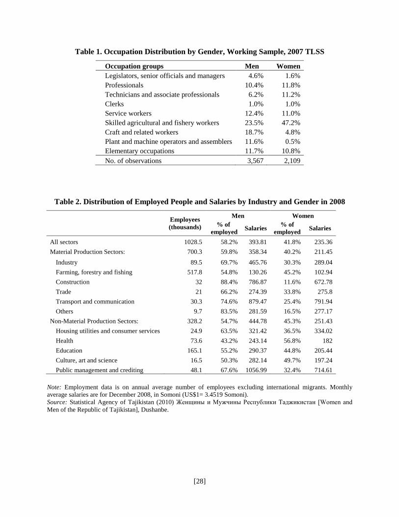
Tajikistan's women also face occupational segregation, working in low-paid sectors, such

as education, health care and agriculture with salaries 4-8 times lower than in industries in which

men predominate (Shahriari, Danzer, Giovarelli, and Undeland, 2009). The TLSS 2007 (see

Table 1) shows that the women are underrepresented in managerial occupations, such as

legislators, senior officials and managers, 1.6% of working women versus to 4.6 % of working

men; in crafts and plant and machine operators 4.8% and 0.5% versus 18.7% and 11.6% for men,

respectively. The major employer of women remains the agricultural sector where they are two

times more represented than men: 47.2% of working women versus 23.5% for working men.

The official data on the distribution of employees and salaries by sectors of the economy

and gender are reported in Table 2. According to this table women are employed less in all

material production sectors of Tajikistan's economy. Tajikistan's women are employed more than

[6]

men in health, and have almost equal employment with men in culture, arts and science.

Furthermore, on average for all sectors, women receive salaries which are 158 Somoni (US$46)

less than men. The highest wage differential is in public management and crediting sectors,

where men receive salaries which are 342 Somoni (US$99) more than women. Almost equal

salaries between men and women are in the trade sector. The only sector where women have a

significant advantage in salaries is in housing utilities and consumer services sectors, where their

salaries are on average 13 Somoni (US$4) larger. In short, women in Tajikistan face segregation

in occupation and industry, and receive significantly lower compensation.

III. Data

Tajikistan provides a good case for studying the roles of massive emigration and education on

domestic labour supply decisions. Since independence in 1991, large numbers of Tajiks have

emigrated and returned, mainly to Russia. This has made Tajikistan the subject of several useful

data collection efforts. We use the data from the 2007 World Bank Living Standard

Measurement Survey on Tajikistan (TLSS 2007). The survey asks questions on both individual

qualities including information about migration experience, and household economic conditions.

The survey was conducted during September and October 2007, with many households revisited

in November.

Our sample includes men and women in their core economically active ages from 25 to

55. We look at the employment decisions of those who were in households that were revisited in

November 2007. Our whole sample size is 10,103 people: 4,662 men and 5,441 women. 76.1%

of respondents in our sample, or 6,926 people, live in rural areas (Rural): 3,244 men and 3,682

women. The respondents from urban areas make-up 23.9% of the whole sample (Urban), or

[7]

3,177 people: 1,418 are men and 1,759 are women. 7.8% of respondents live the capital of

Tajikistan – Dushanbe (RegionD1), 29.4% live in Sogd province (the northern part; RegionD2),

36.7% live in Khatlon province (the south-eastern part; RegionD3), 23.3% live in Regions of

Republican Subordination (around the capital, and further to its east; RegionD4), and 2.8% live

in the highest mountainous (eastern) part of Tajikistan, the Badakhshan area (RegionD5).

Variable definitions are given in Table 3; summary statistics by gender and rural-urban divisions

are reported in Table 4.

Our main variable of interest is LFP which takes a value of 1 if a respondent worked in

the last 14 days including occasional work and zero otherwise. 56.4% of whole sample were

employed in last 14 days, the employment rate in rural is larger than in urban areas, 57.3%

versus 53.6%, respectively. The employment rate among women is significantly lower than that

of men: in the whole sample, 77.2% of men and 37.5% of women worked; while, in rural areas,

the employment of men is 77.4% and that of women is 38.7%, and in urban areas, the

employment of men is 76.5% and of women is smaller, at 33.9%. Higher women employment

rates in rural areas might be driven by two major factors. Firstly, migration is higher in rural

areas, and since it is male dominated, women remaining in these areas have to work in order to

compensate for the absence of their male relatives. Secondly, farming, forestry and fishing

sectors providing almost 50% of jobs in Tajikistan are concentrated in rural areas and have

relatively more female employment. Women (female) are slightly over-represented in our

sample, probably because Tajikistan’s large external migration is male dominated: women

constitute 52.4% of the whole sample, 52% in the rural sample and 53.6% in the urban sample.

The dummy variables for age categories show the decreasing relationship between the number of

people and age. The majority of respondents are 25 to 29, 25.7% of the whole sample, 26.5% of

[8]

the rural sample and 23% of the urban sample. This is not surprising; Tajikistan's population is

overwhelmingly young.

We aim to capture the link between migration and the decision to work (LFP) using two

dummy variables. The first dummy variable Mig_Exp defines individual migration experience.

In our sample, 5.5% of respondents were migrants in last 12 months, predominantly men (10.9%

of the male sample versus 0.7% of the female sample) and from rural areas (5.8% of the rural

sample respondents were migrants or 11.4% of rural men). Respondents from urban areas have

been less involved in migration, 4.6% were migrants in last 12 months, or 9% of the urban male

population.

The second migration variable, Mig_HH, defines whether an individual has a migrant

relative who currently lives in another country. 12.9% of respondents in the whole sample have

at least one relative who currently lives in another country. Since the majority of Tajikistan's

migrants are from the rural areas, respondents from rural areas are more likely to have migrant

relatives than respondents from urban areas, 14.4% of rural versus 8.3% of urban respondents.

Because migrants are predominantly men, households with current migrants have more female

members: in the whole sample, women with current migrants constitute 15.2% while only 10.5%

of men have a current migrant relative. These numbers are higher for the rural sample, 17% of

women and 11.5% of men in these areas have current migrant relatives. However they are lower

for the urban sample, 9.4% of women and 6.9% of men have current migrant relatives.

The education system in Tajikistan consists of pre-school education, general education,

and professional education. Pre-school education is compulsory, however parents have the

option of sending their children to pre-school organizations or educating them at home. General

education is divided into three parts: primary, basic and secondary education. Tajik law requires

[9]

all children at age 7 to attend school, and guarantees their education until age 16. Inherited from

the Soviet era, this system ensures high school attendance rates.

Professional (post-secondary) education is wide-spread in Tajikistan, with 25.1% having

what is referred to as a professional education: 14.2% graduating from special and technical

schools (EducVoc) and 10.9% graduated from universities (EducHigh). The majority of

respondents graduated from secondary general schools (EducGen), 56.5%. 18.4% of respondents

have a primary education (EducPrimary). There is a large difference in educational attainment

between men and women in Tajikistan. On average women are more likely to have primary or

secondary education than men: 24.7% of women and 11.5% of men have primary education and

61.6% of women and 50.9% of men have a secondary general education. However, more men

have professional education than women: 20.8% of men and 8.2% of women have education

from special and technical schools, while 16.8% of men and 5.5% of women have professional

degrees from universities.

On average respondents from rural areas are more likely to have non-professional

education, i.e. education limited to primary (19.5%) or secondary (59.4%) general education.

These numbers are correspondingly 14.9% and 47.2% for the urban sample. Living in urban

areas further increases opportunities to acquire professional education, with 18.6% of the urban

population having professional education from special and technical schools and 19.3% from

universities. The corresponding numbers for rural population are 12.8% and 8.2%. More women

in rural areas lack professional education than women living in urban areas: 26.3% and 64.6% of

rural women have education from primary and secondary general schools, while 19.9% and

52.1% of urban women have such education, respectively. Since professional schools are mainly

concentrated in urban areas in Tajikistan, women living in these areas have a greater chance of

[10]

obtaining professional education than women in rural areas: 15.3% and 12.7% of women in

urban areas have professional education from special and technical schools and universities,

respectively. The corresponding numbers for women in rural areas are 5.9% and 3.2%.

A quarter of respondents in our sample are heads of households (Head), 46.7% of men

and 5.8% of women. The number of household heads is lower in the rural sample, since families

are larger in rural areas of Tajikistan and living in rural areas increases chances of migration for

men including household heads. Furthermore, female headed households are more likely to be

living in urban areas. Most of the respondents in our sample are married (Married), 87.9%. Men

are more likely to be married, 92.3% of men in whole or rural samples, and 92.2% of men in

urban sample are married. Marriage rates are lower for women in urban areas: 80.5% of women

in urban areas and 85% of women in rural areas married.

The majority in our sample are of Tajik ethnicity (Tajik): 75.3% of whole sample, 74.9%

of all men and 75.6% of all women. Relatively more Tajiks are from rural areas: 84% and 72.6%

live in rural and urban areas, respectively. Most of non-Tajiks are Uzbek. Other minority

ethnicities include Russian, Kyrgyz, Tartar, and Turkmen.

Households in our sample have an average size (HHSize) of 8.6 people. Households in

rural areas are relatively larger than household in urban areas: on average, rural households have

9 people, while urban household have 7.6 members. Decomposition into age categories shows

rural households have more children and elders: on average, there are 1.4 children younger than

6 (Child6), 2.4 children between 6-17 (Child6_18), and 0.4 elderly 65 or older (Elder65) in rural

areas, while 1.2 children with age of less than 6, 2 children with 6-17 ages, and 0.2 elders in

urban areas.

[11]

On average monthly non-wage income (OtherIncom1000) is 533 Somoni, generated by

households and including wages of other household members, remittances, scholarships,

transfers, social assistance, income from rent and farming, and other income received by all

household members. Women have more non-wage income than men in all three samples. Non-

wage income is relatively higher for the rural sample, mostly from the inflow of remittances.

More families in rural areas in Tajikistan send migrants abroad, hence they benefit by receiving

additional income in kind: on average, rural families receive monthly non-wage income of 556

Somoni, while urban families receive 458 Somoni.

IV. Determinants of Labour Force Participation

We estimate the effects of individual and family characteristics on individual LFP decisions

using the probit model. Our dependent variable, LFP, takes a value of one if an individual

worked in last 14 days including any occasional work and zero otherwise. Explanatory variables

include individual characteristics such as individual ages, education level, gender, whether he or

she is the head of household, migration experience, ethnicity and marriage, as well as

household's characteristics such as living in urban areas and different country's regions, size of

household, number of children in the household with ages of less than 6, and ages from 6 to 17,

number of elders with ages of older than 65, having a current migrant relative abroad, and the

size of other monthly non-wage income. We estimate probit equations for each of whole, urban

and rural sample. The first equation is estimated for all people in the sample including gender.

The second and third equations are estimated for men and women, respectively. Table 5 reports

probit estimates, as well as the marginal effects of each variable on the probability of LFP, for

[12]

the whole sample. Tables 6 and 7 provide probit estimates and marginal effects for the rural and

urban samples, respectively.

We look at the effect of two factors of our interest, migration and education. Returned

migrants (Mig_Exp = 1) are less likely to be working. The marginal effect of the variable

defining whether an individual was a migrant in last 12 months on the probability of working is

negative and significant. The relationship is strong mainly for men and is not significant for

women; migration in Tajikistan is male dominated, and there are few female migrants in our

sample. The discouragement effect of migration experience in the domestic labour market is

stronger for urban return migrants in comparison to rural returnees: migration experience

significantly reduces the probability of working by urban and rural men of 27.1% and 18.2%,

respectively.

Having a migrant relative who currently works abroad (Mig_HH = 1) reduces the

respondent’s probability of working. The coefficient on the dummy variable defining whether

the household has a current migrant is negative and significant. Having a current migrant in the

family reduces the individual probability of working by 4.7%. Since the income effect of

remittances is captured by other nonwage income, i.e. keeping the effect of remittances constant,

the dummy variable on current migrant reflects the demonstration effect of migration: migrants'

male relatives do not work since they may also plan to migrate observing the benefits of

migration by relatives. Indeed, since Tajikistan's migration is male dominated, having a migrant

relative is not significantly related to the likelihood of working for women, but is significantly

[13]

negative on men’s probability of working. 3 Furthermore, it is mainly rural men whose LFP

decision is impacted by relative’s migration; we do not observe any significant effect of having a

current migrant relative on the likelihood of working for the urban sample. As most migrants are

from the rural areas of Tajikistan, it seems natural to observe a strong demonstration effect of

migration for the rural male sample.

The variables defining the levels of education show an increasing relationship between

education and the probability of working. The reference education level is primary education. At

the sample average, having education from secondary general schools is not significantly

different than primary education. The estimate on the dummy capturing secondary general

education is positive but not significant for the whole sample. After the sample is divided into

urban and rural, the effect of having a secondary general education becomes important for urban

men: its estimate is positive and significant. In other words, men with such education are more

likely to work than those with the lowest (i.e. primary) education in urban areas. Professional

education has a significantly positive effect on the probability of working. Receiving education

from special and technical schools (vocational education) increases the probability of working by

12% for the whole sample – its estimate is positive and significant. Having a higher professional

education further increases the probability of working: a university education increases the

chances of being employment by 22.2% for the whole sample. The effect of professional

education is strong for women, the marginal effects of professional education on the probability

of working doubles for women, but is smaller for men. This finding is persistent in the probit

3 For women, having migrant relatives after controlling remittance is likely to increase labor

market participation because a working member is absent and demonstration effect will be

negligible considering low probability of female migration.

[14]

models estimated using the urban and rural samples. In other words, having professional

education is very important for female LFP. The effect of professional education is stronger for

men living in urban areas than in rural areas: having a special and technical education increases

the probability of working for men living in urban areas by 13.5% and rural areas by 2.6%; and

having a university degree increases such probability by 17.2% and 7.6% in urban and rural

areas, respectively.

For the whole sample, age dummy variables show an inverse-U relationship between the

probability of working and individual age. The reference age is from 25 to 29 years old. Older

respondents are more likely to be working, except those 50 to 55 years old whose coefficient is

negative, though not significant. Being 30-34 years old has a slightly larger positive and

significant effect on working than the reference age. The probability of working is highest for

ages from 35-39, its marginal effect is almost at 10% for the whole sample. The marginal effect

of age on the probability of working reduces to 9.4% for ages 40-44, then to 7% for ages 45-49.

The age effect on the probability of employment is strong mainly for women: the estimates are

significant for women sample estimates for age groups of 35-39, 40-44, and 45-49, but are not

significant for every male age group. A similar pattern can be found when the samples are

divided into rural and urban samples. As men enter the labour force earlier, we do not observe

any significant difference between age categories on the probability of working. However, urban

men at ages 50-55 are more likely to not work in comparison to those 25-29 years old: the

estimate for the 50-55 age category in the urban sample is negative for men and significant. On

the other hand, urban women's participation in the labour force after the age of 35 steadily

increases until the age of 50.

[15]

Heads of Household are more likely to work; its estimate for whole sample is positive

and also significant. The marginal effect is 10.5% for the whole sample. The marginal effect of

being a head on the probability of working is larger for women than men: being a head increases

the chance of employment by 12.8% for women, and 7.8% for men. Such effects are persistent

for both rural and urban samples.

Marriage does not affect the probability of working; the estimate on its dummy variable

is not significant for the whole sample. While for the female sample its probit estimate is

negative and significant – married women are less likely to work. The marriage reduces the

probability of women working by 9.2% for the whole female sample, by 9.9% for the rural

female sample, and 12.8% for the urban female sample. However, being a married man increases

the probability of working; the corresponding estimate for the male sample is positive and

significant across all three samples. Marriage for men increases their probability of working by

18.4% for the whole male sample, 17.8% for the rural male sample, and 21.2% for the urban

male sample.

Ethnic disparity in employment in Tajikistan is also found, though not consistent across

samples. Overall ethnic Tajiks are less likely to work than non-Tajik ethnic groups. The estimate

on the dummy variable on Tajik ethnicity is negative and significant for both whole and rural

samples, but not significant for the urban sample. Tajik women are less likely to work than non-

Tajik women at the whole sample. This effect is strong in rural areas, while showing no

significant difference between Tajik and non-Tajik women's employment in urban areas. The

probability of working is reduced by 7.2% for Tajik women in rural areas. Ethnicity, however,

does not have any effect on men's work decision across all three samples.

[16]

Living in urban areas is associated with reduction in probability of working. The estimate

on the dummy of living in an urban area for all people is negative and significant. The effect of

this variable is stronger for women than for men: living in the urban area reduces the probability

of working of women by 8.2%, significant, and of men by 3.5%, significant. Regional

differences on LFP are significant. People in Khatlon province and Regions of Republican

Subordination are more likely to work than those who live in the capital (Dushanbe) for the

whole sample. Their corresponding marginal effects on the probability of working are 9.2%, and

5%, respectively. These regional effects are stronger for women than for men: living in Khatlon

province and Regions of Republican Subordination increases the probability of working for

women by 21.6% and 5.8%, respectively. Both areas were torn by the civil war, and are largely

dependent on agricultural production. While living in Sogd and Badakhshan for the whole

sample does not have a significant effect on employment comparatively to those who live in the

capital. However, when men and women are separately estimated, living in Badakhshan

increases probability of working by 8.8% for women, but reduces it by 14.4% for men.

For the rural sample, the reference group is Sogd province. Compared to the rural areas

of Sogd province, living in Khatlon province increases the probability of working by 23.8% for

women, but reduces it by 5.9% for men. Though smaller, positive and significant effects are

found for living in rural areas of Regions of Republican Subordination and Badakhshan province

for women. There is no difference for men in working in rural areas of Sogd Province and

Regions of Republican Subordination. While men living in rural areas of Badakhshan province

are less likely to work: the marginal effect on the probability of working is negative (-15.6%)

and significant.

[17]

In the urban sample, living in Sogd province increases the probability of women working

but not men relative to living in the capital (Dushanbe). For women, living in urban areas of

Sogd province increases the likelihood of working by 16.5% compared to those living in the

capital. Living in urban areas of Badakhshan province increases the probability of working by

16.2% for women and reduces it by 20.7% for men compared to those living in the capital.

However, living in urban areas of Khatlon province and Regions of Republican Subordination

for both men and women do not have any significant impact on the likelihood of working

relative to those living in the capital.

Household size does not have any significant effect on the probability of working for the

whole sample. When estimated by gender, the effect is significant for men but not for women.

An increase in household size reduces the probability of working for men; the estimate is

negative and significant. However, when the model is estimated by rural and urban, size of

household has significantly positive effect for only women in urban areas.

The number of children with ages less than 6 years old decreases the probability of

working. The estimate is negative and significant. This effect is strong for women and

significant, but not significant for men. Women with young children choose not to work and look

after their children, once children become older, parents decide to return to work again. The

effect of number of children with ages of younger than 6 years old is stronger for women in

urban than rural areas. An additional child younger than 6 years old lowers the probability of

working by 7.1% and 2.4% for women living in urban and rural areas, respectively.

Furthermore, the number of children in ages of 6 to 17 and the number of elders with

ages 65 and older do not have any significant impact on the probability of working for the whole

and rural samples. However, for the urban sample, number of elders reduces the probability of

[18]

working by 6% for women, but does not have any significant impact on men. The number of

children in ages of 6 to 17 also does not have any impact on working for both men and women in

urban areas.

Other non-wage income has a positive and significant, though small, impact on the

employment probability for the whole sample. However, when we look at subgroups, the

positive effect is found only for men living rural areas. Since poverty is high in Tajikistan, most

families are likely to keep working despite the additional income they receive from other sources

including remittances.

In the probit equations when a pooled sample of men and women is used, gender

disparity is captured by the female categorical variable. Its coefficient estimate is negative and

statistically significant. Keeping the effect of other individual and household characteristics

constant, women are less likely to work by 36.1% for the whole sample, 36% for the rural

sample, and 38.2% for the urban sample. This specification is restrictive in the sense that it

constrains men and women to have the same coefficients for all explanatory variables except for

the intercept. In the next section, we study the gender gap in LFP rates utilizing the probit

estimates for separate samples which do not have any restriction on the estimates of the models.

It is quite plausible that labour force participation (LFP) and migration decision

(Mig_Exp) are correlated, i.e., Mig_Exp is an endogenous variable in the LFP equation. This

issue is widely recognized, but is not easy to overcome due to various conceptual and data issues.

Nonetheless we have estimated a bivariate probit model for men and women to account for the

potential endogeneity of the migration variable in the LFP decision. The results for the men and

[19]

women in the whole sample are reported in the Table Appendix.4 Focusing on the results for

men, the bivariate probit estimates of LFP equation are not qualitatively much different from

those of single probit estimates reported in Table 5. This may be quite natural considering that

the correlation coefficient (𝜌) is close to zero. We also find this in bivariate estimations for men

in rural and urban samples. Though these results do not completely resolve the endogeneity

issues, we use single probit estimates in decomposition analysis since bivariate probit estimation

is hard to obtain for the women’s sample due to the small sample size of female migrants, and it

is desirable to have the same econometric models for men and women in decomposition analysis.

V. Decomposing the Gender Gap in Labour Force Participation

Using Oaxaca type decomposition of differences in binary variables, we explain the gender gap

in LFP in Tajikistan. Oaxaca (1973) and Blinder (1973) introduced regression based

decomposition for studying differences between groups. We use the decomposition method

proposed by Yun (2004; 2005b; 2008) for discrete dependant variables. The likelihood of

participating in the labour force for individual 𝑖 is estimated by Φ(𝑋𝑖𝛽), where 𝑋𝑖 is a 1 ×

𝑘 vector of explanatory variables, 𝛽 is a 𝑘 × 1 vector of coefficients, and Φ is a standard normal

cumulative distribution function. The observed LFP rate is asymptotically equal to sample

average of the individual likelihood of LFP:

𝐿𝐹𝑃����� = Φ(𝑋𝛽)��������� =1N�Φ(𝑋𝑖𝛽).𝑁

𝑖=1

4 A major problem with our bivariate probit is the very small sample of women who migrated,

which causes difficulty in estimating the bivariate probit model when rural and urban samples

are separately studied.

[20]

Algebraically, the difference in the average likelihoods of LFP between male (A) and

female (B) may be decomposed as:

𝐿𝐹𝑃�����𝐴 − 𝐿𝐹𝑃�����𝐵 = � Φ(𝑋𝐴𝛽𝐴)����������� − Φ(𝑋𝐵𝛽𝐴)������������ � + � Φ(𝑋𝐵𝛽𝐴)������������ − Φ(𝑋𝐵𝛽𝐵)������������ �,

where the first and the second components on the right-hand side represent the "characteristics

effect" and "coefficients effect", respectively; and an "over bar" represents the value of the

sample’s average.

This decomposition provides us with the overall characteristics and coefficients effects.

In order to find the relative contribution of each variable to the gender gap in LFP, in terms of

characteristics and coefficients effects, we employ a decomposition equation for the probit

model as proposed by Yun (2004):

𝐿𝐹𝑃�����𝐴 − 𝐿𝐹𝑃�����𝐵 = �𝑊∆𝑋𝑗

𝑘

𝑗=1

� Φ(𝑋𝐴𝛽𝐴)����������� − Φ(𝑋𝐵𝛽𝐴)������������ �+ �𝑊∆𝛽𝑗

𝑘

𝑗=1

� Φ(𝑋𝐵𝛽𝐴)������������ − Φ(𝑋𝐵𝛽𝐵)������������ � ,

where 𝑊∆𝑋𝑗 =

�𝑋�𝐴𝑗−𝑋�𝐵

𝑗 �𝛽𝐴𝑗

(𝑋�𝐴−𝑋�𝐵)𝛽𝐴 , 𝑊∆𝛽

𝑗 =𝑋�𝐵𝑗 �𝛽𝐴

𝑗−𝛽𝐵𝑗 �

𝑋�𝐵(𝛽𝐴−𝛽𝐵) , and ∑ 𝑊∆𝛽𝑗𝑘

𝑗=1 = ∑ 𝑊∆𝑋𝑗𝑘

𝑗=1 = 1, while 𝑋�𝐴𝑗 and 𝑋�𝐵

𝑗

are average values of explanatory variable 𝑗 for groups 𝐴 and 𝐵, respectively.5

5 For computing asymptotic standard errors of the characteristics and coefficients effects, see Yun (2005a).

Robustness issues, known as the index or parameterization problem and the identification problem, have

been dealt with in the detailed decompositions. A decomposition equation with a different parameterization

[ (Φ(X_A β_A ) ) ̅- (Φ(X_B β_A ) ) ̅ ]+ [ (Φ(X_B β_A ) ) ̅- (Φ(X_B β_B ) ) ̅ ] was computed; the results

are not substantially different. Another interpretation issue is that the coefficients effect in the detailed

decomposition is not invariant to the choice of omitted groups when dummy variables are used (Oaxaca and

Ransom, 1999). The solution suggested by Yun (2005b; 2008) is used here: as alternative reference groups

yield different estimates of the coefficients effects for each individual variable, it is natural to obtain

estimates of the coefficients effects for every possible omission and take the average of the coefficients

effects estimates as the “true” contributions of individual variables to differentials. This can be accomplished

[21]

The decomposition results based on normalized equations suggested in Yun (2005b, 2008)

are reported in Table 8, 9 and 10 for all three samples: the whole, rural and urban samples. Our

main focus is on the estimated percentage share which defines the major contributions to the

gender gap in LFP. The method decomposes the predicted differences in the LFP rates of women

and men into characteristics and coefficients effects. 6 For the whole sample, the overall

(aggregate) characteristics effect accounts for 9.1% of the total gender gap of 39.7%, whereas the

overall coefficients effect accounts for 90.9% of the total gender gap. Both characteristics and

coefficients effects are significant. These results suggest that the gender gap in LFP is less

dependent on the differences in male and female characteristics, but is largely driven by

behavioural differences (probit coefficients) between men and women. Though equalizing

attributes between men and women will help reduce the gender gap in LFP, it is not likely to be

reduced substantially unless women act more like men (or men act like women) in Tajikistan.

Both rural and urban samples also show that most of the gender gap in LFP is explained by the

coefficients effect: the characteristics and coefficients effects are 14.4% and 85.7%, respectively,

for urban sample, and 6.5% and 93.5%, respectively, for rural sample. All characteristics and

coefficients effects are significant except for the characteristics effect for rural sample, which is

significant.

with a single estimation by transforming the probit estimates into a normalized equation and using the

normalized equation for the decomposition. 6 The predicted gender gap of LFP is 39.7% (=77.2% - 37.5%) for the whole sample, 38.7%

(=77.4% - 38.7%) for rural sample, and 42.7% (=76.5% - 33.8%) for urban sample, respectively.

The observed gender gaps of LFP are 39.7%, 38.7%, and 42.6% for the whole sample, rural

sample, and urban sample, respectively.

[22]

For the detailed decomposition, we focus on the contribution of migration and education

to the gender gap in LFP. First, look at the migration variables. The probit estimates of

migration variables (Mig_Exp and Mig_HH) indicate that they tend to decrease the likelihood of

participation. There is a huge gap in own migration experience between men and women since

Tajikistan's migration is male dominated. This leads to a negative characteristics effect for

having migration experience (Mig_Exp), meaning that the LFP gender gap would be widened if

the gender gap in migration experience disappears, i.e., if male dominance in migration

disappears. On the other hand, the characteristics effect of having migrant relatives (Mig_HH) is

positive because women have larger responses to having relatives who have migrated. If this

disparity disappears, then the LFP gender gap narrows. The coefficients effects of both Mig_Exp

and Mig_HH are negative (e.g., -0.0008 and -0.0031, respectively, for the whole sample),

however, only the coefficients effect of own migration experience (Mig_Exp) is significant; these

results indicate that the participation discouraging effects of these variables are stronger for men.

This seems natural considering that most of migrants are male in Tajikistan. Hence, if the

discouragement effect of migration is equalized between men and women, the gender gap of LFP

is widened.

Next we look at the detailed decomposition for the education variables. Overall, both

characteristics and coefficients effects of education variables are positive. This means that if the

differences in educational attainments and their participation enhancing effects disappear, the

gender gap in LFP shrinks. From the mean characteristics given in Table 4, we show that, on

average, men have better educational attainment, particularly vocational and university education.

Therefore, it is necessary for more women to participate in vocational and university education

in order to reduce the gender gap in LFP. This finding is reinforced as the participation

[23]

increasing effects of vocational and university education are much stronger for women. This

leads to negative coefficients effects of these education levels (EducVoc and EducHigh), while

the coefficients effects of other education variables (EducPrimary and EducGen) are positive.

VI. Conclusion

Tajikistan – a small and landlocked country – underwent a serious economic and political

transformation after independence from the Soviet Union in 1991. Over the last two decades it

evolved into the world’s most migrant remittance dependent country with much of its labour

force working abroad (mainly Russia). At the same time, Tajikistan has a well-developed

educational system which, while not free from discrimination, leans that way. Tajikistan

provides a good case for studying the roles of massive emigration and education on domestic

labour supply decisions. With samples from World Bank Living Standard Measurement Survey

on Tajikistan in 2007, we study the correlates of LFP and its gender gap.

Using probit and decomposition analysis, we find that education and migration have a

significant and important relationship with the gender gap in LFP in Tajikistan. That is,

international migration, mainly by men, reduces participation by men domestically, while

women’s education increases female participation; both women's greater access to education,

particularly to higher education, and increased international migration contribute to reducing the

gender gap.

Access to higher education increases employment opportunities for women. Since

professional education schools are mainly concentrated in urban areas, the primary policy

implication of our result might be to expand the accessibility of such education to women either

by providing scholarships for young women to accomplish studies at universities, or encourage

[24]

opening new universities or branches in rural areas. We also find that Tajikistan's men are more

responsive to migration and are more likely than women to leave the labour force. Where there is

significant emigration, male migration might shrink the gender gap in LFP but at the cost of

reducing of the male labour supply and the overall employment.

[25]

References

Abdulloev, I. (2013) Impact of Migration on Job Satisfaction, Professional Education and the Informal Sector. PhD Dissertation, Rutgers University, New Brunswick, NJ.

Acosta, P. (2006) Labor Supply, School Attendance, and Remittances from International Migration: the Case of El Salvador. The World Bank Policy Research Working Paper Series 3903, doi:10.1596/1813-9450-3903.

Amuedo-Dorantes, C. and Pozo, S. (2006) Migration, Remittances, and Male and Female Employment Patterns. American Economic Review 96(2): 222–226.

Becker, G. (1991) A Treatise on the Family. Enlarged ed. Cambridge, MA: Harvard University Press.

Blinder, A. (1973) Wage Discrimination: Reduced Form and Structural Estimates. Journal of Human Resources 8(4): 436–455.

Blunch, N.-H. (2010) The Gender Earnings Gap Revisited: A Comparative Study for Serbia and Five Countries in Eastern Europe and Central Asia. Retrieved from: http://siteresources.worldbank.org/INTECA/Resources/GenderEarningsGap.pdf

Cabegin, E. C. (2006) The Effect of Filipino Overseas Migration on the Non-Migrant Spouse’s Market Participation and Labor Supply Behavior. IZA Discussion Paper No. 2240. Retrieved from: http://ftp.iza.org/dp2240.pdf.

Cunningham, W. (2001) Breadwinner or Caregiver? How Household Role Affects Labor Choices in Mexico. In: E. Katz and M. Correia (eds.) The Economics of Gender in Mexico: Work, Family, State, and Market. Washington, D.C.: World Bank, pp. 85-132.

Goldin, C. (1995) The U-Shaped Female Labor Force Function in Economic Development and Economic History. In: T.P. Schultz (ed.) Investment in Women's Human Capital and Economic Development. Chicago, IL: University of Chicago Press, pp. 61–90.

Hadi, A. (2001) International Migration and the Change of Women's Position among the Left-Behind in Rural Bangladesh. International Journal of Population Geography 7: 53–61.

Hondagneu-Sotelo, P. (1992) Overcoming Patriarchal Constraints: The Reconstruction of Gender Relations among Mexican Immigrant Women and Men. Gender and Society 6(3): 393–415.

Killingsworth, M. and Heckman, J. (1987) Female labor supply: A survey. In: in O. Ashenfelter and R. Layard (eds) Handbook of Labor Economics. Elsevier, edition 1, volume 1, number 1, pp. 103–204.

[26]

Klasen, S. and Pieters, J. (2012) Push or Pull? Drivers of Female Labor Force Participation during India’s Economic Boom. IZA Discussion Paper No. 6395. Retrieved from: http://ftp.iza.org/dp6395.pdf.

Mammen, K. and Paxson, C. (2000) Women's Work and Economic Development. Journal of Economic Perspectives 14(4): 141-164.

Mincer, J. (1974) Schooling, Experience, and Earnings. National Bureau of Economic Research Books, Inc. Retrieved from: http://EconPapers.repec.org/RePEc:nbr:nberbk:minc74–1.

Neumark, D. and McLennan, M. (1995) Sex Discrimination and Women's Labor Market Outcomes. The Journal of Human Resources 30(4), 713–740.

Nguyen, T. and Purnamasari, R. (2011) Impacts of International Migration and Remittances on Child Outcomes and Labor Supply in Indonesia: How Does Gender Matter? The World Bank Policy Research Working Paper Series, No 5591, doi:10.1596/1813-9450-5591.

Oaxaca, R. (1973) Male-Female Wage Differentials in Urban Labor Markets. International Economic Review 14(3): 693–709.

Oaxaca, R. and Ransom, M. (1999) Identification in Detailed Wage Decompositions. The Review of Economics and Statistics 81(1): 154–157.

Paris, T., Singh, A., Luis, J. and Hossain, M. (2005) Labour Outmigration, Livelihood of Rice Farming Households and Women Left Behind: A Case Study in Eastern Uttar Pradesh. Economic and Political Weekly 40(25): 2522–2529.

Rodriguez, E. and Tiongson, E. (2001) Temporary Migration Overseas and Household Labor Supply: Evidence from Urban Philippines. International Migration Review 35(3): 709–725.

Safarova, M., Abdurakhmanova, A. and Kasymova, R. (2007) A Gender Analysis of EU Development Instruments and Policies in Tajikistan Representing Central Asia. EU Gender Watch: Dushanbe, Khujand. Retrieved from: http://www.neww.org.pl/download/EU_GenderWatch_Tajikistan.pdf

Semyonov, M. (1980) The Social Context of Women's Labor Force Participation: A Comparative Analysis. American Journal of Sociology 86(3): 534–550.

Shahriari, H., Danzer, A. M., Giovarelli, R., & Undeland, A. (2009) Improving Women’s Access to Land and Financial Resources in Tajikistan. World Bank Group Gender Action Plan Report. Washington, DC: World Bank.

Signorelli, M., Choudhry, M. and Marelli, E. (2012) The Impact of Financial Crises on Female Labour. European Journal of Development Research 24: 413–433.

[27]

Statistical Agency of Tajikistan (2010) Женщины и Мужчины Республики Таджикистан [Women and Men of the Republic of Tajikistan]. Dushanbe: Statistical Agency of Tajikistan.

Statistical Agency of Tajikistan (2011) Database. Available at: http://stat.tj/ru/database/real-sector/ [Accessed 17 September 2011].

Statistical Committee of CIS (2011) Average Monthly Nominal Wage in the CIS Countries, in national currency. Available at: http://www.cisstat.com/index.html [Accessed 17 September 2011].

World Bank (2011) Migration and Remittances. Factbook 2011. Second edition. Available at: http://siteresources.worldbank.org/INTLAC/Resources/Factbook2011-Ebook.pdf [Accessed 12 August 2011].

World Bank (2013) World Data Bank. Available at: http://databank.worldbank.org/data/home.aspx [Accessed 17 May 2013].

Yun, M.-S. (2004) Decomposition Differences in the First Moment. Economics Letters 82(2): 273–278.

Yun, M.-S. (2005a) Hypothesis Tests When Decomposing Differences in the First Moment. Journal of Economic and Social Measurement 30(4): 295–304.

Yun, M.-S. (2005b) A Simple Solution to the Identification Problem in Detailed Wage Decomposition. Economic Inquiry 43(4): 766–772.

Yun, M.-S. (2008) Identification Problem and Detailed Oaxaca Decomposition: A General Solution and Inference. Journal of Economic and Social Measurement 33(1): 27–38.

[28]

Table 1. Occupation Distribution by Gender, Working Sample, 2007 TLSS

Occupation groups Men Women Legislators, senior officials and managers 4.6% 1.6% Professionals 10.4% 11.8% Technicians and associate professionals 6.2% 11.2% Clerks 1.0% 1.0% Service workers 12.4% 11.0% Skilled agricultural and fishery workers 23.5% 47.2% Craft and related workers 18.7% 4.8% Plant and machine operators and assemblers 11.6% 0.5% Elementary occupations 11.7% 10.8% No. of observations 3,567 2,109

Table 2. Distribution of Employed People and Salaries by Industry and Gender in 2008

Employees (thousands)

Men Women

% of employed Salaries % of

employed Salaries

All sectors 1028.5 58.2% 393.81 41.8% 235.36 Material Production Sectors: 700.3 59.8% 358.34 40.2% 211.45

Industry 89.5 69.7% 465.76 30.3% 289.04 Farming, forestry and fishing 517.8 54.8% 130.26 45.2% 102.94 Construction 32 88.4% 786.87 11.6% 672.78 Trade 21 66.2% 274.39 33.8% 275.8 Transport and communication 30.3 74.6% 879.47 25.4% 791.94 Others 9.7 83.5% 281.59 16.5% 277.17

Non-Material Production Sectors: 328.2 54.7% 444.78 45.3% 251.43 Housing utilities and consumer services 24.9 63.5% 321.42 36.5% 334.02 Health 73.6 43.2% 243.14 56.8% 182 Education 165.1 55.2% 290.37 44.8% 205.44 Culture, art and science 16.5 50.3% 282.14 49.7% 197.24 Public management and crediting 48.1 67.6% 1056.99 32.4% 714.61

Note: Employment data is on annual average number of employees excluding international migrants. Monthly average salaries are for December 2008, in Somoni (US$1= 3.4519 Somoni). Source: Statistical Agency of Tajikistan (2010) Женщины и Мужчины Республики Таджикистан [Women and Men of the Republic of Tajikistan], Dushanbe.

[29]

Table 3. Definitions of Variables used in Regressions LFP Dummy variable taking a value of 1 if worked in last 14 days including occasional work Male Dummy variable taking a value of 1 if an individual is male Female Dummy variable taking a value of 1 if an individual is female Age25_29 Dummy variable taking a value of 1 if an individual's age is between 25-29 Age30_34 Dummy variable taking a value of 1 if an individual's age is between 30-34 Age35_39 Dummy variable taking a value of 1 if an individual's age is between 35-39 Age40_44 Dummy variable taking a value of 1 if an individual's age is between 40-44 Age45_49 Dummy variable taking a value of 1 if an individual's age is between 45-49 Age50_55 Dummy variable taking a value of 1 if an individual's age is between 50-55 Mig_Exp Dummy variable taking a value of 1 if an individual was a migrant in last 12 months EducPrimary Dummy variable taking a value of 1 if an individual has the highest degree from a primary

school EducGen Dummy variable taking a value of 1 if an individual has the highest degree from the general

secondary school EducVoc Dummy variable taking a value of 1 if an individual has the highest degree from technical

or special school EducHigh Dummy variable taking a value of 1 if an individual has the highest degree from university Head Dummy variable taking a value of 1 if an individual is the head of the household Married Dummy variable taking a value of 1 if an individual is married Tajik Dummy variable taking a value of 1 if an individual has a Tajik ethnicity Rural Dummy variable taking a value of 1 if an individual lives in a rural area Urban Dummy variable taking a value of 1 if an individual lives an urban area RegionD1 Regional dummy taking value of 1 if individual lives in the capital (Dushanbe) RegionD2 Regional dummy taking value of 1 if individual lives in Sogd province RegionD3 Regional dummy taking value of 1 if individual lives in Khatlon province RegionD4 Regional dummy taking value of 1 if individual lives in any of Regions of Republican

Subordination RegionD5 Regional dummy taking value of 1 if individual lives in Badakhshan province HHSize Size of the household Child6 Number of children in the household with ages of less than 6 years old Child6_18 Number of children in the household with ages of greater of equal to 6 but less than 18

years old Elder65 Number of elders with age of 65 and older Mig_HH Dummy variable taking a value of 1 if a household has a current migrant abroad OtherIncom1000 Monthly other non-wage income in thousands of Somoni (total household income minus

individual work earnings).

[30]

Table 4. Summary Statistics: Whole, Rural and Urban Samples

Variables Whole sample Rural sample Urban sample

All Men Women All Men Women All Men Women Mean SD Mean SD Mean SD Mean SD Mean SD Mean SD Mean SD Mean SD Mean SD

LFP 0.564 0.496 0.772 0.420 0.375 0.484 0.573 0.495 0.774 0.418 0.387 0.487 0.536 0.499 0.765 0.424 0.339 0.473 Age25_29 0.257 0.437 0.256 0.436 0.258 0.438 0.265 0.442 0.265 0.442 0.265 0.441 0.230 0.421 0.223 0.416 0.236 0.424 Age30_34 0.191 0.393 0.200 0.400 0.183 0.386 0.189 0.392 0.199 0.399 0.180 0.384 0.197 0.398 0.204 0.403 0.190 0.393 Age35_39 0.150 0.357 0.147 0.354 0.152 0.359 0.144 0.351 0.146 0.353 0.142 0.349 0.169 0.374 0.152 0.359 0.183 0.386 Age40_44 0.138 0.345 0.139 0.346 0.137 0.344 0.138 0.344 0.135 0.341 0.140 0.347 0.140 0.347 0.155 0.362 0.127 0.333 Age45_49 0.130 0.336 0.130 0.337 0.130 0.336 0.130 0.337 0.132 0.338 0.129 0.335 0.129 0.335 0.127 0.333 0.131 0.338 Age50_55 0.134 0.341 0.127 0.333 0.141 0.348 0.134 0.340 0.124 0.329 0.143 0.350 0.136 0.343 0.139 0.346 0.133 0.340 Mig_Exp 0.055 0.229 0.109 0.311 0.007 0.084 0.058 0.235 0.114 0.318 0.007 0.082 0.046 0.209 0.090 0.286 0.008 0.088 EducPrimary 0.184 0.388 0.115 0.319 0.247 0.431 0.195 0.396 0.122 0.327 0.263 0.440 0.149 0.356 0.091 0.288 0.199 0.399 EducGen 0.565 0.496 0.509 0.500 0.616 0.486 0.594 0.491 0.538 0.499 0.646 0.478 0.472 0.499 0.415 0.493 0.521 0.500 EducVoc 0.142 0.349 0.208 0.406 0.082 0.275 0.128 0.334 0.203 0.402 0.059 0.236 0.186 0.389 0.224 0.417 0.153 0.360 EducHigh 0.109 0.311 0.168 0.374 0.055 0.228 0.082 0.275 0.137 0.344 0.032 0.175 0.193 0.395 0.270 0.444 0.127 0.333 Head 0.253 0.435 0.467 0.499 0.058 0.235 0.235 0.424 0.445 0.497 0.042 0.200 0.309 0.462 0.539 0.498 0.111 0.314 Married 0.879 0.326 0.923 0.267 0.839 0.368 0.885 0.319 0.923 0.266 0.850 0.358 0.859 0.348 0.922 0.269 0.805 0.396 Tajik 0.753 0.431 0.749 0.433 0.756 0.429 0.726 0.446 0.721 0.449 0.730 0.444 0.840 0.367 0.842 0.364 0.837 0.369 Rural 0.761 0.426 0.767 0.423 0.755 0.430 Urban 0.239 0.426 0.233 0.423 0.245 0.430 RegionD1 0.078 0.268 0.073 0.259 0.083 0.276 - - - - - - 0.327 0.469 0.312 0.463 0.339 0.473 RegionD2 0.294 0.456 0.297 0.457 0.291 0.454 0.293 0.455 0.294 0.456 0.292 0.455 0.298 0.457 0.309 0.462 0.288 0.453 RegionD3 0.367 0.482 0.374 0.484 0.360 0.480 0.404 0.491 0.409 0.492 0.399 0.490 0.250 0.433 0.259 0.438 0.242 0.429 RegionD4 0.233 0.423 0.229 0.420 0.236 0.425 0.272 0.445 0.268 0.443 0.275 0.447 0.110 0.312 0.103 0.304 0.115 0.319 RegionD5 0.028 0.166 0.027 0.161 0.030 0.170 0.032 0.176 0.030 0.169 0.034 0.182 0.016 0.125 0.017 0.128 0.015 0.123 HHSize 8.647 3.400 8.780 3.407 8.527 3.390 8.972 3.333 9.083 3.337 8.870 3.326 7.613 3.406 7.782 3.445 7.466 3.365 Child6 1.396 1.366 1.445 1.388 1.352 1.345 1.446 1.383 1.489 1.401 1.407 1.366 1.235 1.297 1.300 1.334 1.179 1.262 Child6_18 2.287 1.536 2.245 1.532 2.324 1.539 2.384 1.544 2.338 1.535 2.426 1.550 1.977 1.469 1.938 1.479 2.011 1.460 Elder65 0.357 0.618 0.368 0.628 0.346 0.608 0.391 0.644 0.405 0.655 0.378 0.633 0.249 0.511 0.249 0.509 0.248 0.513 Mig_HH 0.129 0.336 0.105 0.306 0.152 0.359 0.144 0.351 0.115 0.319 0.170 0.376 0.083 0.276 0.069 0.254 0.094 0.293 OtherIncom1000 0.533 0.811 0.463 0.791 0.597 0.824 0.556 0.858 0.492 0.849 0.616 0.862 0.458 0.633 0.365 0.546 0.539 0.689 No. of Samples 10,103 4,662 5,441 6,926 3,244 3,682 3,177 1,418 1,759

[30]

Table 5. Probit Estimates and Marginal Effects: Whole Sample and by Gender (Dependent variable: worked in last 14 days, LFP)

Variables Probit Estimates Marginal Effects All Men Women All Men Women

Age30_34 0.1484 *** 0.1140

0.0873

0.0573 0.0323 0.0331 (0.0523) (0.0832) (0.0719) (0.0199) (0.0229) (0.0275) Age35_39 0.2590 *** 0.0669

0.3447 *** 0.0987 0.0191 0.1335

(0.0615) (0.0983) (0.0793) (0.0227) (0.0276) (0.0312) Age40_44 0.2478 *** 0.0339

0.3245 *** 0.0945 0.0098 0.1256

(0.0622) (0.1081) (0.0782) (0.0230) (0.0309) (0.0308) Age45_49 0.1840 *** 0.0677

0.2378 *** 0.0707 0.0193 0.0916

(0.0618) (0.1072) (0.0791) (0.0232) (0.0300) (0.0310) Age50_55 -0.0311

-0.1671

0.0570

-0.0122 -0.0510 0.0216

(0.0614) (0.1089) (0.0782) (0.0241) (0.0347) (0.0298) Mig_Exp -0.5423 *** -0.5889 *** 0.0768

-0.2136 -0.1986 0.0292

(0.0747) (0.0750) (0.2531) (0.0284) (0.0279) (0.0974) EducGen 0.0670

0.1318

0.0076

0.0262 0.0384 0.0028

(0.0435) (0.0819) (0.0533) (0.0170) (0.0239) (0.0200) EducVoc 0.3190 *** 0.1780 ** 0.5904 *** 0.1206 0.0497 0.2311 (0.0599) (0.0907) (0.0849) (0.0216) (0.0242) (0.0331) EducHigh 0.6239 *** 0.3703 *** 1.0635 *** 0.2224 0.0970 0.4021 (0.0690) (0.0978) (0.0991) (0.0213) (0.0227) (0.0321) Female -0.9633 *** - - -0.3613 - - (0.0429) (0.0148) Head 0.2747 *** 0.2699 *** 0.3294 *** 0.1053 0.0780 0.1283 (0.0525) (0.0861) (0.0892) (0.0196) (0.0246) (0.0355) Married -0.0307

0.5457 *** -0.2400 *** -0.0120 0.1843 -0.0923

(0.0522) (0.0915) (0.0644) (0.0203) (0.0343) (0.0251) Tajik -0.1113 *** 0.0171

-0.2019 *** -0.0432 0.0050 -0.0770

(0.0399) (0.0611) (0.0526) (0.0154) (0.0179) (0.0203) Urban -0.1483 *** -0.1169 * -0.2229 *** -0.0583 -0.0349 -0.0819 (0.0458) (0.0703) (0.0634) (0.0181) (0.0214) (0.0227) RegionD2 0.0982

0.0607

0.1229

0.0382 0.0175 0.0466

(0.0600) (0.0973) (0.0832) (0.0232) (0.0277) (0.0318) RegionD3 0.2388 *** -0.1267

0.5667 *** 0.0925 -0.0373 0.2156

(0.0607) (0.0961) (0.0819) (0.0232) (0.0288) (0.0312) RegionD4 0.1290 ** 0.1321

0.1521 * 0.0500 0.0374 0.0579

(0.0629) (0.1039) (0.0861) (0.0241) (0.0285) (0.0331) RegionD5 -0.0653

-0.4310 *** 0.2279 ** -0.0257 -0.1438 0.0882

(0.0698) (0.1065) (0.0945) (0.0276) (0.0393) (0.0374) HHSize -0.0021

-0.0294 * 0.0053

-0.0008 -0.0086 0.0020

(0.0100) (0.0165) (0.0132) (0.0039) (0.0048) (0.0050) Child6 -0.0513 ** 0.0094

-0.0910 *** -0.0200 0.0027 -0.0342

(0.0216) (0.0350) (0.0290) (0.0084) (0.0102) (0.0109) Child6_18 0.0214

0.0415

0.0296

0.0084 0.0121 0.0111

(0.0163) (0.0263) (0.0214) (0.0064) (0.0076) (0.0081) Elder65 -0.0085

0.0218

-0.0187

-0.0033 0.0064 -0.0070

(0.0296) (0.0485) (0.0399) (0.0116) (0.0141) (0.0150) Mig_HH -0.1190 *** -0.1945 ** -0.0818

-0.0469 -0.0600 -0.0304

(0.0462) (0.0764) (0.0597) (0.0183) (0.0248) (0.0220) OtherIncome1000 0.0464 ** 0.1396 *** 0.0148

0.0181 0.0407 0.0056

(0.0210) (0.0453) (0.0282) (0.0082) (0.0131) (0.0106) Constant 0.4325 *** 0.1601

-0.4826 *** - - -

(0.1135) (0.1722) (0.1348) N 10,103 4,662 5,441

Pseudo R2 0.1601 0.0653 0.0842

For all tables below, standard errors in parentheses, * p<.10, ** p<.05, *** p<.01

[31]

Table 6. Probit Estimates and Marginal Effects: Rural Sample and by Gender (Dependent variable: worked in last 14 days, LFP)

Variables Probit Estimates Marginal Effects All Men Women All Men Women

Age30_34 0.1516 ** 0.1250

0.1000

0.0582 0.0351 0.0384 (0.0610) (0.0956) (0.0829) (0.0231) (0.0260) (0.0320) Age35_39 0.2588 *** 0.0805

0.3878 *** 0.0979 0.0228 0.1515

(0.0732) (0.1139) (0.0943) (0.0268) (0.0315) (0.0373) Age40_44 0.2562 *** 0.1097

0.3306 *** 0.0969 0.0307 0.1290

(0.0732) (0.1296) (0.0918) (0.0267) (0.0351) (0.0363) Age45_49 0.1650 ** 0.1417

0.1929 ** 0.0631 0.0393 0.0747

(0.0720) (0.1265) (0.0928) (0.0270) (0.0335) (0.0364) Age50_55 -0.0022

-0.0649

0.0398

-0.0009 -0.0192 0.0152

(0.0712) (0.1340) (0.0892) (0.0277) (0.0403) (0.0342) Mig_Exp -0.5218 *** -0.5458 *** -0.0412

-0.2058 -0.1815 -0.0156

(0.0837) (0.0847) (0.2905) (0.0323) (0.0310) (0.1090) EducGen 0.0360

0.0630

-0.0006

0.0140 0.0183 -0.0002

(0.04920 (0.0920) (0.0605) (0.0191) (0.0267) (0.0230) EducVoc 0.2062 *** 0.0907

0.4764 *** 0.0785 0.0257 0.1874

(0.0724) (0.1042) (0.1104) (0.0268) (0.0289) (0.0435) EducHigh 0.5084 *** 0.2879 ** 1.0686 *** 0.1827 0.0762 0.4002 (0.0923) (0.1181) (0.1570) (0.0295) (0.0282) (0.0485) Female -0.9639 ***

-0.3600

(0.0509) (0.0175) Head 0.2658 *** 0.2284 ** 0.3094 *** 0.1012 0.0654 0.1212 (0.0641) (0.1044) (0.1202) (0.0238) (0.0295) (0.0479) Married -0.0290

0.5319 *** -0.2544 *** -0.0112 0.1785 -0.0988

(0.0632) (0.1076) (0.0775) (0.0244) (0.0401) (0.0305) Tajik -0.1148 *** 0.0009

-0.1870 *** -0.0444 0.0003 -0.0719

(0.0440) (0.0669) (0.0578) (0.0169) (0.0194) (0.0224) RegionD3 0.2334 *** -0.1999 ** 0.6245 *** 0.0901 -0.0587 0.2380 (0.0495) (0.0785) (0.0667) (0.0189) (0.0232) (0.0249) RegionD4 0.0951 * 0.0758

0.1451 ** 0.0368 0.0217 0.0557

(0.0515) (0.0884) (0.0714) (0.0198) (0.0250) (0.0275) RegionD5 -0.1089 * -0.4645 *** 0.1750 ** -0.0428 -0.1556 0.0679 (0.0613) (0.0930) (0.0827) (0.0242) (0.0340) (0.0325) HHSize -0.0099

-0.0297

-0.0054

-0.0039 -0.0086 -0.0020

(0.0117) (0.0191) (0.0152) (0.0045) (0.0056) (0.0058) Child6 -0.0399

-0.0023

-0.0638 * -0.0155 -0.0007 -0.0243

(0.0250) (0.0404) (0.0331) (0.0097) (0.0117) (0.0126) Child6_18 0.0359 * 0.0484

0.0397

0.0140 0.0140 0.0151

(0.0190) (0.0304) (0.0249) (0.0074) (0.0088) (0.0095) Elder65 0.0051

0.0151

0.0049

0.0020 0.0044 0.0018

(0.0329) (0.0536) (0.0443) (0.0128) (0.0155) (0.0168) Mig_HH -0.1445 *** -0.2160 ** -0.0886

-0.0567 -0.0666 -0.0334

(0.0517) (0.0852) (0.0672) (0.0204) (0.0277) (0.0251) OtherIncome1000 0.0479 ** 0.1458 *** 0.0199

0.0186 0.0422 0.0076

(0.0226) (0.0502) (0.0309) (0.0088) (0.0144) (0.0118) Constant 0.5288 *** 0.2974 * -0.4345 ***

(0.1169) (0.1755) (0.1353) N 6,926 3,244 3,682

Pseudo R2 0.1520 0.0638 0.0819

[32]

Table 7. Probit Estimates and Marginal Effects: Urban Sample and by Gender (Dependent variable: worked in last 14 days, LFP)

Variables Probit Estimates Marginal Effects All Men Women All Men Women

Age30_34 0.1626 * 0.0614

0.1305

0.0638 0.0178 0.0473 (0.0988) (0.1619) (0.1415) (0.0384) (0.0461) (0.0520) Age35_39 0.2913 *** -0.0070

0.3419 ** 0.1131 -0.0021 0.1268

(0.1097) (0.1853) (0.1493) (0.0414) (0.0546) (0.0570) Age40_44 0.2509 ** -0.2122

0.4358 *** 0.0976 -0.0658 0.1642

(0.1150) (0.1870) (0.1494) (0.0436) (0.0609) (0.0582) Age45_49 0.2800 ** -0.1635

0.4808 *** 0.1085 -0.0502 0.1817

(0.1203) (0.1971) (0.1590) (0.0453) (0.0630) (0.0621) Age50_55 -0.1179

-0.4252 ** 0.1427

-0.0468 -0.1385 0.0519

(0.1205) (0.1848) (0.1683) (0.0480) (0.0653) (0.0625) Mig_Exp -0.5998 *** -0.7712 *** 0.4351

-0.2332 -0.2706 0.1664

(0.1657) (0.1607) (0.4682) (0.0600) (0.0622) (0.1864) EducGen 0.2013 ** 0.4179 ** 0.0428

0.0795 0.1190 0.0152

(0.0930) (0.1767) (0.1129) (0.0366) (0.0488) (0.0401) EducVoc 0.6379 *** 0.5212 *** 0.7349 *** 0.2379 0.1351 0.2799 (0.1070) (0.1848) (0.1372) (0.0363) (0.0419) (0.0529) EducHigh 0.8777 *** 0.6700 *** 1.0699 *** 0.3156 0.1719 0.4061 (0.1078) (0.1826) (0.1374) (0.0330) (0.0405) (0.0489) Female -1.0102 ***

-0.3820

(0.0775) (0.0268) Head 0.3079 *** 0.3251 ** 0.2977 ** 0.1204 0.0962 0.1108 (0.0913) (0.1516) (0.1438) (0.0350) (0.0449) (0.0555) Married -0.0922

0.6158 *** -0.3455 *** -0.0363 0.2118 -0.1280

(0.0908) (0.1764) (0.1195) (0.0356) (0.0673) (0.0456) Tajik -0.0366

0.0969

-0.1722

-0.0145 0.0292 -0.0628

(0.0901) (0.1424) (0.1178) (0.0355) (0.0440) (0.0440) RegionD2 0.2993 *** 0.0902

0.4486 *** 0.1170 0.0261 0.1651

(0.0761) (0.1201) (0.0994) (0.0290) (0.0341) (0.0380) RegionD3 0.0575

-0.0564

0.1386

0.0227 -0.0167 0.0501

(0.0817) (0.1237) (0.1137) (0.0322) (0.0372) (0.0419) RegionD4 0.1372

0.1516

0.0994

0.0539 0.0424 0.0360

(0.0928) (0.1567) (0.1267) (0.0360) (0.0415) (0.0466) RegionD5 -0.0628

-0.5941 *** 0.4255 *** -0.0249 -0.2073 0.1624

(0.1172) (0.1585) (0.1529) (0.0466) (0.0615) (0.0607) HHSize 0.0271

-0.0337

0.0495 * 0.0107 -0.0099 0.0176

(0.0192) (0.0319) (0.0254) (0.0076) (0.0094) (0.0091) Child6 -0.0886 ** 0.0617

-0.1993 *** -0.0351 0.0181 -0.0709

(0.0408) (0.0608) (0.0586) (0.0161) (0.0179) (0.0207) Child6_18 -0.0406

0.0282

-0.0245

-0.0161 0.0083 -0.0087

(0.0318) (0.0516) (0.0420) (0.0126) (0.0152) (0.0149) Elder65 -0.0803

0.0473

-0.1693 * -0.0318 0.0139 -0.0602

(0.0657) (0.1067) (0.0935) (0.0260) (0.0313) (0.0334) Mig_HH -0.0165

-0.0849

-0.0099

-0.0065 -0.0256 -0.0035

(0.0961) (0.1578) (0.1290) (0.0381) (0.0489) (0.0457) OtherIncome1000 0.0348

0.0726

0.0067

0.0138 0.0213 0.0024

(0.0540) (0.1124) (0.0659) (0.0214) (0.0330) (0.0234) Constant 0.0592

-0.2652

-0.8157 ***

(0.1884) (0.2794) (0.2192) N 3,177 1,418 1,759

Pseudo R2 0.2022 0.0864 0.1395

[33]

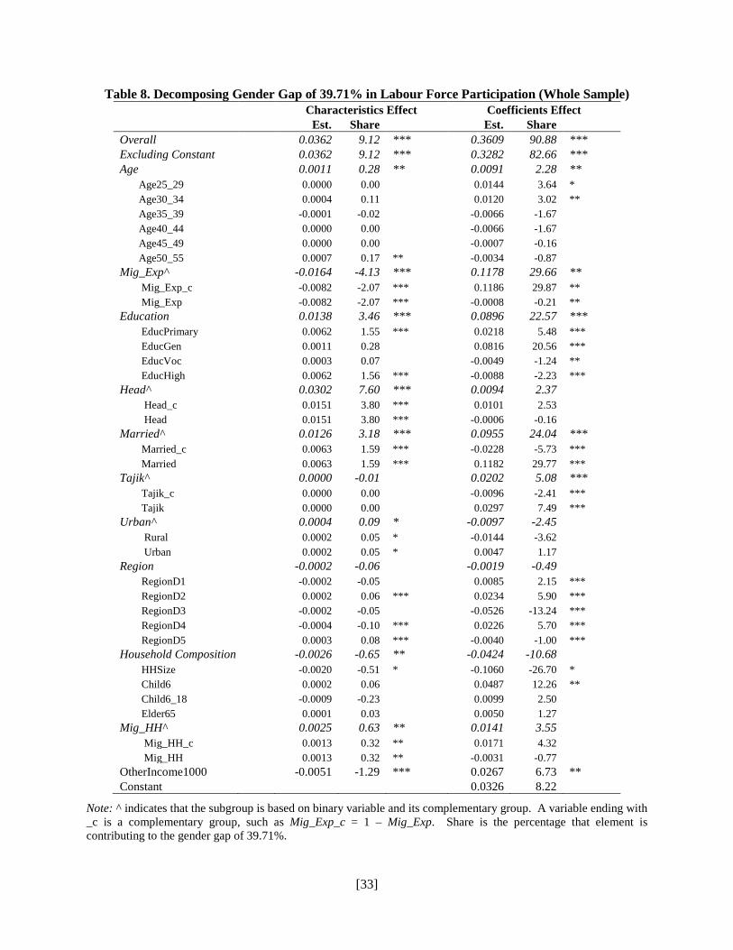
Table 8. Decomposing Gender Gap of 39.71% in Labour Force Participation (Whole Sample)

Characteristics Effect Coefficients Effect

Est. Share

Est. Share

Overall 0.0362 9.12 *** 0.3609 90.88 *** Excluding Constant 0.0362 9.12 *** 0.3282 82.66 *** Age 0.0011 0.28 ** 0.0091 2.28 ** Age25_29

0.0000 0.00

0.0144 3.64 *

Age30_34

0.0004 0.11

0.0120 3.02 ** Age35_39

-0.0001 -0.02

-0.0066 -1.67

Age40_44

0.0000 0.00

-0.0066 -1.67 Age45_49

0.0000 0.00

-0.0007 -0.16

Age50_55

0.0007 0.17 ** -0.0034 -0.87 Mig_Exp^ -0.0164 -4.13 *** 0.1178 29.66 **

Mig_Exp_c

-0.0082 -2.07 *** 0.1186 29.87 ** Mig_Exp

-0.0082 -2.07 *** -0.0008 -0.21 **

Education 0.0138 3.46 *** 0.0896 22.57 *** EducPrimary

0.0062 1.55 *** 0.0218 5.48 ***

EducGen

0.0011 0.28

0.0816 20.56 *** EducVoc

0.0003 0.07

-0.0049 -1.24 **

EducHigh

0.0062 1.56 *** -0.0088 -2.23 *** Head^ 0.0302 7.60 *** 0.0094 2.37

Head_c

0.0151 3.80 *** 0.0101 2.53 Head

0.0151 3.80 *** -0.0006 -0.16

Married^ 0.0126 3.18 *** 0.0955 24.04 *** Married_c

0.0063 1.59 *** -0.0228 -5.73 ***

Married 0.0063 1.59 *** 0.1182 29.77 *** Tajik^ 0.0000 -0.01

0.0202 5.08 ***

Tajik_c

0.0000 0.00

-0.0096 -2.41 *** Tajik

0.0000 0.00

0.0297 7.49 ***

Urban^ 0.0004 0.09 * -0.0097 -2.45 Rural

0.0002 0.05 * -0.0144 -3.62

Urban

0.0002 0.05 * 0.0047 1.17 Region -0.0002 -0.06

-0.0019 -0.49

RegionD1

-0.0002 -0.05

0.0085 2.15 *** RegionD2

0.0002 0.06 *** 0.0234 5.90 ***

RegionD3

-0.0002 -0.05

-0.0526 -13.24 *** RegionD4

-0.0004 -0.10 *** 0.0226 5.70 ***

RegionD5

0.0003 0.08 *** -0.0040 -1.00 *** Household Composition -0.0026 -0.65 ** -0.0424 -10.68

HHSize

-0.0020 -0.51 * -0.1060 -26.70 * Child6

0.0002 0.06

0.0487 12.26 **

Child6_18

-0.0009 -0.23

0.0099 2.50 Elder65

0.0001 0.03

0.0050 1.27

Mig_HH^ 0.0025 0.63 ** 0.0141 3.55 Mig_HH_c

0.0013 0.32 ** 0.0171 4.32

Mig_HH

0.0013 0.32 ** -0.0031 -0.77 OtherIncome1000 -0.0051 -1.29 *** 0.0267 6.73 **

Constant

0.0326 8.22 Note: ^ indicates that the subgroup is based on binary variable and its complementary group. A variable ending with

_c is a complementary group, such as Mig_Exp_c = 1 – Mig_Exp. Share is the percentage that element is contributing to the gender gap of 39.71%.

[34]

Table 9. Decomposing Gender Gap of 38.72% in Labour Force Participation (Rural Sample)

Characteristics Effect Coefficients Effect

Est. Share

Est. Share

Overall 0.0253 6.53 ** 0.3619 93.47 *** Excluding Constant 0.0253 6.53 ** 0.3285 84.85 *** Age 0.0010 0.25

0.0065 1.67

Age25_29

0.0000 0.00

0.0104 2.69 Age30_34

0.0003 0.07

0.0087 2.24

Age35_39

0.0000 0.00

-0.0100 -2.58 ** Age40_44

-0.0001 -0.02

-0.0056 -1.44

Age45_49

0.0001 0.01

0.0027 0.70 Age50_55

0.0007 0.17

0.0003 0.07

Mig_Exp^ -0.0155 -3.99 *** 0.0888 22.94 * Mig_Exp_c

-0.0077 -2.00 *** 0.0894 23.10 *

Mig_Exp

-0.0077 -2.00 *** -0.0006 -0.16 * Education 0.0096 2.49 * 0.0961 24.81 *** EducPrimary

0.0041 1.06

0.0259 6.68 ***

EducGen

0.0014 0.35

0.0782 20.21 *** EducVoc

-0.0007 -0.19

-0.0023 -0.60

EducHigh

0.0049 1.27 ** -0.0057 -1.47 *** Head^ 0.0242 6.26 ** 0.0133 3.42

Head_c

0.0121 3.13 ** 0.0139 3.58 Head

0.0121 3.13 ** -0.0006 -0.16

Married^ 0.0103 2.67 *** 0.0981 25.33 *** Married_c

0.0052 1.34 *** -0.0211 -5.45 ***

Married

0.0052 1.34 *** 0.1192 30.78 *** Tajik^ 0.0000 0.00

0.0154 3.99 **

Tajik_c

0.0000 0.00

-0.0090 -2.33 ** Tajik

0.0000 0.00

0.0245 6.32 **

Region -0.0001 -0.03

0.0049 1.26 RegionD2

0.0001 0.02 *** 0.0399 10.30 ***

RegionD3

-0.0001 -0.04

-0.0627 -16.20 *** RegionD4

-0.0004 -0.12 *** 0.0309 7.97 ***

RegionD5

0.0004 0.11 *** -0.0031 -0.81 *** Household Composition -0.0027 -0.70 ** -0.0371 -9.59

HHSize

-0.0017 -0.43

-0.0769 -19.87 Child6

0.0000 -0.01

0.0309 7.98

Child6_18

-0.0011 -0.29

0.0075 1.95 Elder65

0.0001 0.03

0.0014 0.36

Mig_HH^ 0.0031 0.81 ** 0.0150 3.87 Mig_HH_c

0.0016 0.40 ** 0.0189 4.87

Mig_HH

0.0016 0.40 ** -0.0039 -1.00 OtherIncome1000

-0.0047 -1.22 *** 0.0276 7.14 **

Constant

0.0334 8.62 Note: ^ indicates that the subgroup is based on binary variable and its complementary group. A variable ending with

_c is a complementary group, such as Mig_Exp_c = 1 – Mig_Exp. Share is the percentage that element is contributing to the gender gap of 38.72%.

[35]

Table 10. Decomposing Gender Gap of 42.72% in Labour Force Participation (Urban Sample)

Characteristics Effect Coefficients Effect

Est. Share

Est. Share

Overall 0.0613 14.35 *** 0.3659 85.65 *** Excluding Constant 0.0613 14.35 *** 0.4373 102.36 *** Age -0.0019 -0.44

0.0211 4.93 ***

Age25_29

-0.0004 -0.10

0.0312 7.30 ** Age30_34

0.0007 0.17

0.0206 4.83 **

Age35_39

-0.0010 -0.24

0.0020 0.46 Age40_44

-0.0007 -0.17

-0.0119 -2.78 *

Age45_49

0.0001 0.01

-0.0121 -2.83 * Age50_55

-0.0005 -0.12 ** -0.0087 -2.05

Mig_Exp^ -0.0183 -4.28 *** 0.2069 48.44 ** Mig_Exp_c

-0.0091 -2.14 *** 0.2086 48.82 **

Mig_Exp

-0.0091 -2.14 *** -0.0016 -0.39 ** Education 0.0254 5.95 *** 0.0598 13.99 *** EducPrimary

0.0124 2.91 *** 0.0041 0.97

EducGen

-0.0005 -0.11

0.0790 18.48 *** EducVoc

0.0024 0.57

-0.0082 -1.92

EducHigh

0.0110 2.58 *** -0.0151 -3.53 *** Head^ 0.0402 9.40 ** -0.0037 -0.87

Head_c

0.0201 4.70 ** -0.0042 -0.99 Head

0.0201 4.70 ** 0.0005 0.12

Married^ 0.0208 4.86 *** 0.1021 23.90 *** Married_c

0.0104 2.43 *** -0.0327 -7.66 ***

Married

0.0104 2.43 *** 0.1348 31.56 *** Tajik^ 0.0001 0.03

0.0316 7.40

Tajik_c

0.0001 0.02

-0.0076 -1.79 Tajik

0.0001 0.02

0.0393 9.19

Region -0.0005 -0.11

0.0503 11.77 *** RegionD1

-0.0006 -0.15

0.0360 8.42 ***

RegionD2

0.0011 0.25 * -0.0054 -1.27 RegionD3

0.0001 0.03

0.0092 2.16

RegionD4

-0.0008 -0.20 * 0.0143 3.35 ** RegionD5

-0.0002 -0.04 *** -0.0038 -0.89 ***

Household Composition -0.0015 -0.35

-0.0538 -12.58 HHSize

-0.0031 -0.72

-0.2168 -50.74 **

Child6

0.0022 0.50

0.1073 25.12 *** Child6_18

-0.0006 -0.14

0.0370 8.65

Elder65

0.0000 0.00

0.0187 4.39 Mig_HH^ 0.0006 0.14

0.0106 2.48

Mig_HH_c

0.0003 0.07

0.0118 2.77 Mig_HH

0.0003 0.07

-0.0012 -0.29

OtherIncome1000

-0.0037 -0.86

0.0124 2.90 Constant

-0.0714 -16.71

Note: ^ indicates that the subgroup is based on binary variable and its complementary group. A variable ending with _c is a complementary group, such as Mig_Exp_c = 1 – Mig_Exp. Share is the percentage that element is contributing to the gender gap of 42.72%.

[36]

Table Appendix. Bivariate Probit Estimates: Labour Force Participation and Migration

Men Women LFP Mig_Exp LFP Mig_Exp

Age30_34 0.0931

0.0936

0.1435 ** 0.1227

0.0697

0.0835

0.0603

0.2153

Age35_39 0.0459

0.0160

0.3163 *** 0.3588

0.0814

0.1021

0.0659

0.2309

Age40_44 0.0831

-0.0568

0.3963 *** 0.0330

0.0898

0.1088

0.0657

0.2264

Age45_49 0.0574

-0.1915 * 0.2996 *** -0.4575

0.0899

0.1101

0.0662

0.2867

Age50_55 -0.1329

-0.4749 *** 0.1329 ** -0.5542 **

0.0936

0.1172

0.0652

0.2543

Mig_Exp -0.5731

1.7787 ***

0.3968

0.6607

EducGen 0.1451 ** 0.2638 *** 0.0449

-0.0511

0.0709

0.0954

0.0458

0.1667

EducVoc 0.1902 ** 0.2505 ** 0.5682 *** 0.4684 **

0.0793

0.1065

0.0693

0.1866

EducHigh 0.4623 *** 0.0242

1.0609 *** 0.0772

0.0819

0.1130

0.0778

0.2495

Head 0.2939 *** 0.1715 * 0.3768 *** 0.1009

0.0705

0.0894

0.0740

0.2663

Married 0.4842 *** 0.0757

-0.2106 *** -0.0009

0.0734

0.1042

0.0533

0.1658

Tajik 0.0931 * 0.0907

-0.1630 *** -0.1507

0.0535

0.0641

0.0453

0.1247

Urban -0.1882 *** -0.1523 ** -0.2106 *** -0.0130

0.0601

0.0769

0.0522

0.1814

RegionD2 -0.0021

0.2238 ** 0.1240 * 0.1016

0.0859

0.1117

0.0716

0.1950

RegionD3 -0.1285

0.4177 *** 0.5133 *** -0.1138

0.0892

0.1117

0.0716

0.2145

RegionD4 0.0208

0.2753 ** 0.1093

-0.2077

0.0911

0.1172

0.0740

0.2330

RegionD5 -0.5210 *** -0.5933 *** 0.1668 ** -5.5908 ***

0.0956

0.1544

0.0809

0.2704

HHsize -0.0317 ** 0.0120

0.0138

0.1176 ***

0.0142

0.0178

0.0112

0.0292

Child6 0.0429

-0.0921 *** -0.0964 *** -0.3053 ***

0.0293

0.0353

0.0248

0.0879

Child6_18 0.0520 ** -0.0280

0.0204

-0.1560 ***

0.0225

0.0277

0.0182

0.0543

Elder65 0.0538

-0.1272 ** 0.0085

-0.0533

0.0408

0.0551

0.0339

0.1059

Mig_HH -0.1698 *** -0.0023

-0.0318

0.2671 *

0.0632

0.0858

0.0489

0.1620

OtherIncome1000 0.1043 *** 0.0333

0.0095

0.1070 **

0.0380

0.0322

0.0257

0.0427

Constant 0.1371

-1.7236 *** -0.6091 *** -2.7182 ***

0.1411

0.1934

0.1110

0.3509

/athrho -0.0280 -0.8756**

0.1994 0.4053

𝜌 -0.0280 -0.7042** Note: /athrho is defined as 0.5ln((1+ ρ)/(1- ρ)), where ρ is the correlation coefficient of error terms in two equations of LFP and Mig_Exp. Wald test for ρ =0 is not significant at 10% level for men, and significant at 5% level for women.