Microsoft Excel Handbook
33
COMPUTER TRAINING Michele Marinucci Learning Microsoft Excel
-
Upload
muzamil-ahmad -
Category
Education
-
view
441 -
download
4
Transcript of Microsoft Excel Handbook

COMPUTER TRAINING Michele Marinucci
Learning
Microsoft Excel

Table of ContentsWhat is Excel?........................................................................... 1 How Can Excel Help Me? ......................................................... 1 The Excel Screen...................................................................... 2 Using the Lingo ......................................................................... 2 Using the Menu Bar................................................................... 3
File .................................................................................................. 3 Using the File Commands............................................................... 5 Edit.................................................................................................. 6 Working with the Edit Commands ................................................... 7 View ................................................................................................ 8 Using the Viewing Options .............................................................. 9 Insert ............................................................................................. 10 Using the Insert Commands.......................................................... 11 Format........................................................................................... 12 Using the Format Commands ....................................................... 13 Tools ............................................................................................. 14 Using the Tool Commands............................................................ 15 Data .............................................................................................. 16 Window ......................................................................................... 17 Help............................................................................................... 18
Formulas ................................................................................. 19 Using the Formula bar................................................................... 19 Writing Basic Formulas ................................................................. 20 Writing Basic Formulas ................................................................. 23
Formatting Your Worksheet/Workbook ................................... 24 Adding color to the text or worksheet ............................................ 24 Printing specific rows or columns on each page ........................... 24 Fitting to one page ........................................................................ 24
Charting your Data .................................................................. 25 A Step by Step Guide.................................................................... 25 Charting Your Data ....................................................................... 27
Chart Types and Examples ..................................................... 28 Keyboard Shortcuts................................................................. 29 Other Helpful Sites .................................................................. 30

Chapter
1 L E A R N I N G M I C R O S O F T E X C E L
What is Excel? Spreadsheet Solutions to Make Your Job Easier
icrosoft Excel is a spreadsheet program that is based on a table format. In other words, it is simply a big collection of rows and columns into which you can enter numbers, words, pictures and sounds. Think of it as a big calculator meant to make your life easier.
M How Can Excel Help Me? You can use Microsoft Excel to do so many things… Depending upon your interest and your needs, you will have to determine how Excel can work for you. Some of the nifty things that people use Excel for include:
• Calenda
• Timelin
• Flowcha
rs
es rts
• Managing lists (i.e. Customer Management List; Response; Supply List)
• Expense Reports
• Profit/Loss Statements
• General Accounting Ledgers
• Charts and Graphs
1

L E A R N I N G M I C R O S O F T E X C E L
The Excel Screen To open Excel, either click on the Excel icon (if it is located on your desktop) or click Start, Programs, and Microsoft Excel. When you open Microsoft Excel, you will see the new workbook screen (See Figure 1). Generally, this screen opens with 3 tabs at the bottom (known as worksheets). Each sheet is labeled in numerical order. (Ex. Sheet1, Sheet2, Sheet3…).
Figure 1 Using the Lingo Knowing certain terms will make your exploration with Microsoft Excel even easier. Some basic terms and their meanings are listed below.
Cell Each individual “box” in the worksheet; named by using the grid location (A1 refers to the cell that is in Column A, Row 1)
Column The vertical boxes in the worksheet; named by using letters of the alphabet. The first 26 are named A-Z, column 27 is named using AA…
Formula The mathematical command that you want to occur within the cell. Always begins with an = sign.
Menu bar A group of commands, including file, edit, view, which allows the user to perform tasks.
Row The horizontal boxes in the worksheet, named by using numbers
Toolbar The collection of buttons (usually with icons), which provide shortcuts to tasks; typically located at the top of the screen.
Workbook The larger collection of worksheets--You may have one workbook called “Expenses” that contains a worksheet for each month.
Worksheet The page in which all entries are made; Contained within a workbook; named by the tab at the bottom of the worksheet.
2

Using the Menu Bar The menu bar is typically located along the top of the screen. In Microsoft Excel, it includes commands grouped into categories. These categories include:
If you already use Microsoft products, like Microsoft Word, you are probably already familiar with many of the commands available on the menu bar.
File The most common uses for the file set of commands are:
New—create a new workbook
Open—open an existing workbook
Close—close a workbook that you have already opened
Save—save the workbook that you created or have worked on
Save as—save the workbook using a new name or in a new location
Page setup—adjust the margins, header/footer or sheet settings
Print area—after you have highlighted the cells that you want to print, click print area, then click “set print area” and only the highlighted cells will print. To clear the print area, click file, print area, and “clear print area”
Print preview—allows you to view the worksheet as it will print. Tip: This is a great place to adjust all the page settings!!
Updated 9/6/2007
3

•• Start Microsoft Excel.
• Enter the following data into your worksheet: Source: DelDOT Division of Motor Vehicles
A B C D E1 Year of Registration 2 Type of Vehicle 2000 2001 2002 20033 Passenger Car 378,175 382,898 389,400 393,3044 Station Wagon 124,177 130,968 140,132 151,8345 Commercial 129,986 130,508 133,331 136,1406 Farm Truck 2,875 2,888 2,877 2,8667 Recreational 6,577 6,324 6,211 6,0168 Trailer 55,853 58,223 30,382 63,0489 Motorcycle 11,625 12,722 13,721 15,31810 Other 8,084 8,676 9,217 9,489
Updated 9/6/2007
4

Lesson 1 Objectives: 1. Create a new workbook
2. Save the workbook
3. Close the workbook
4. Open a pre-existing workbook
5. Use the print preview settings to:
a. Adjust the page settings
b. Adjust the margins
c. Insert a header and footer
d. Set rows to repeat at the top of each page
Using the File Commands 1. Save your file to your user drive.
2. Close your workbook.
3. Open your workbook.
4. Click on Page-Setup
5. Print Preview your worksheet in both the portrait and landscape
orientations.
6. Select the Margin tab, click to center your worksheet horizontally, then
preview.
7. Select the Header/Footer tab.
a. Click on the button that says “Custom Header…” and type the
following in the center section: “DelDOT Registration Data”, click
OK.
b. Click on the down arrow next to Footer and select the one that
includes your name and the date.
Updated 9/6/2007
5

Edit There are many important commands that fall under the edit heading.
Undo—allows you to undo what you just did. Usually you can undo repeatedly.
Repeat—the opposite of undo, repeat allows you to redo the same action over again.
Cut—takes out the selected cell entry
Copy—makes a copy of the selected cell entry
Paste—use this command if you cut out a cell entry and want to put it in a new location. For example, if you have data in cell A1 and want to move it to cell B2, you would highlight cell A1, click cut, then highlight cell B2 and click paste.
Fill—useful if you are entering a lot of the same information; for example, if you are putting in the number 2 in all cells in column A, you would enter the number into cell A1, click on cell A1, select fill and down and the rest of the cells in column A will fill in with the number 2.
Clear—you can use this command to clear the contents (what you typed) or the formatting (how it looks)
Delete—allows you to remove the data in a cell, a group of cells, remove a row or a column.
Delete sheet—allows you to remove an entire sheet
Move/copy sheet—allows you to rearrange your workbook by reordering your worksheets or copying selected worksheets
Find—a useful command for finding specific data
Replace—allows you to change specific data to something else. For example, if I am working on a spreadsheet and use the name Marinucci throughout the spreadsheet, I can click replace and change every entry of Marinucci to Michele Marinucci.
Updated 9/6/2007
6

Lesson 2 Objectives: Undo an action
Repeat an action
Cut, copy and paste data
Fill cells across
Delete data in cells
Find and replace text in cells
Working with the Edit Commands 1. Highlight cells B2 through E2; click Edit, Fill, and Right. You should
notice that the all of the cells now say 2000.
2. Click Edit, Undo (You can also click the undo button on the toolbar, which
looks like an arrow pointing back to the left).
3. Click on Edit, the Find and type: "Car," click Replace, and type Vehicle in
the replace box. Then select Replace All. This will change cell A3 to say
Passenger Vehicle instead of Passenger Car.
4. Click on Edit, then GoTo and type: D3 then press return. Your cursor now
is located in cell D3.
5. Highlight cell B1 then click Edit, Copy. The cell now should have a dotted
line rotating around it—this means it is selected for copying. Now
highlight cells C1 through E1, click Edit, and Paste. The label Year of
Registration is now at the top of all of the cells. Press the ESC key to stop
the copy feature.
Updated 9/6/2007
7

View Normal View—just that…the normal way the spreadsheet opens and appears
Page break Preview—allows you to see dotted lines showing where the page breaks will occur.
In the picture on the left, you can see what a worksheet looks like using the page break preview. You can adjust the page breaks by clicking and dragging the dotted line to the left or right. When you release the mouse, the view will be updated to show your changes. To change back to normal view, just click view and select normal.
Toolbars—allows you to select the specific toolbars that you want displayed at the top of the screen. Depending upon the tasks you are performing, you can customize your toolbars. Standard and Formatting are the two frequently used toolbars.
Formula Bar—Allows you to view the formula bar. This bar makes writing a formula easier since it allows you to select the type of formula (ex: sum, average…) and will guide you through the formula-writing process.
Header/Footer—allows you to insert a custom or pre-designed header or footer to print at the top (header) or bottom (footer) of each page. You can choose from automatic entries, such as the time or date, or customize so that the title of your report shows on each page.
Comments—Allows you to view a comment/ similar to a sticky note in a cell. The comment will not show up on the cell, but a small red triangle will appear so that you know a comment exists for that cell. To see the comment, just move your mouse over that cell. (To create a comment, click insert, comment.)
Zoom—Allows you to change the size of the display.
A worksheet shown in Page break Preview
Once you press the = button, a drop down menu appears. By clicking on the down arrow, a list of common formulas appears. If the formula type you want is there, just click on it; otherwise, click More Functions.
Updated 9/6/2007
8

Lesson 3 Objectives Adjust page breaks in page break preview
Customize the toolbar
View the formula bar
View the header and footer
Use the zoom feature to adjust the display size on the screen
Using the Viewing Options
1. Click View, then Page Break View. You will see that your worksheet
now appears smaller with a dark blue outline. If your workbook
contained enough information to continue onto more pages, there would
be a dotted blue line separating the pages. These lines are movable to
adjust page breaks. Click View, Normal to return to the Normal view.
2. Click View, Toolbars and make sure that Standard and Formatting are
checked. You can adjust which toolbars are displayed by selecting or
deselecting the toolbar.
3. Click View, Toolbars, Customize, Commands, Format, and scroll down
to find the Merge and Center icon.
a. Click on the icon and drag it up to the toolbar. When a line
appears to the left of the icon, you can let go and it will be
permanently placed on the toolbar.
b. Highlight Cells B1 through E1, then click the merge and center
button that you just added to the toolbar. Since you have data in
all cells, a warning appears. Press OK to continue merging.
4. Click View, Zoom and change to zoom percentage to 200%. This will
change the size of the worksheet that you view on the screen, but NOT
on paper.
Updated 9/6/2007
9

Insert
Cells—Allows you to insert one cell, a row of cells or a column of cells
Rows—Allows you to insert a row of cells
Column—Allows you to insert a column of cells
Worksheet—Allows you to insert a worksheet. (A shortcut is to right click on the tab of an existing worksheet, click insert, and then select worksheet.)
Chart—opens the chart wizard which guides you through the chart creation process
Comment—creates a comment similar to a sticky note. Useful for noting information that might otherwise be forgotten. Can be viewed by moving the mouse over the red triangle. (See view: comment)
Picture—provides you with the option of inserting a clipart picture, a picture from a file, or an organizational chart. The picture does not fit in one cell, but covers a group of cells depending on its size.
Hyperlink—creates a link to a target website or file.
Updated 9/6/2007
10

Lesson 4 Objectives: Insert a row of cells
Insert a new worksheet
Insert a comment
Insert a picture using clipart
Using the Insert Commands 1. Click on the 3 so that the entire row is highlighted, then click Insert,
Row. A new row should appear above the row you highlighted.
2. Click insert, Worksheet.
a. A new sheet should appear, named Sheet4.
b. Double click the tab named “Sheet 4”, and then type
“Averages”. Press enter.
c. The tab name should now say Averages.
d. To rearrange the sheets, click and drag the tab to a new location.
e. Rename Sheet 1 by double clicking the tab name. Type “Reg
Info” and press Enter.
3. Click on cell A1 in the Reg Info sheet. Click Insert, Comment. Type
the following in the yellow box: from DelDOT DMV. Press Enter.
You will notice a small triangle in the top right corner of cell A1. This
indicates that a comment goes with the cell. You can view the comment
by moving your mouse over the cell A1.
4. Click Insert, Picture, ClipArt. Select a picture and either (a) right click
and press Insert OR (b) click on the picture and press the top button that
appears (looks like an arrow going down). The picture you insert floats
on top of the cells and can be moved by dragging the picture or resized
by dragging the corners.
Updated 9/6/2007
11

Format
Cells—adjusts the way the cell appears. Many choices exist here!
If you are working with money and want the decimal place to show, you can click on the number tab and select currency.
The alignment tab allows you to adjust the horizontal and vertical display and allows you to wrap text (have it fit onto two lines if necessary) or shrink to fit in the cell.
Row—adjusts the size of the row’s height and allows you to use the Auto Fit option.
Column—adjusts the size of the column’s width and allows you to use the Auto Fit option.
AutoFormat—changes the format of the entire sheet to match a pre-set option. Highlight the cells you want to apply the formatting to, click format, auto format, and select the appearance option you prefer. The changes will only apply to the selected cells. To apply the formatting to the entire worksheet, click edit, select all before clicking on auto format.
Style—apply formatting options to the entire sheet based upon your pre-selected settings.
Updated 9/6/2007
12

Lesson 5 Objectives Adjust the cell information, including the alignment, format, font, size
and border.
Adjust the row settings
Adjust the column settings
Use the AutoFormat feature
Using the Format Commands
1. Highlight cells B4 through E11, then click Format, and Cells. Select the
tab titled Alignment, change the vertical and horizontal text alignment
to center. Press OK.
2. Highlight rows 1 and 2, then click Format, and Cells. Select the tab
titled Font. Change the style to Bold Italic and a size 14. Click the tab
titled Border and click on the box titled Outline. Click the tab titled
Patterns and select a yellow color. Then click on the dropdown box
next to the word Pattern and select one of the striped patterns. Press
OK.
3. Select the entire table and click Format, Row, and AutoFit.
4. Select the entire table and click Format, Column, and AutoFit.
5. Select the entire table, click Format, AutoFormat, select one of the
choices by clicking on the example and clicking OK
Updated 9/6/2007
13

Tools Spelling—this is the same as Microsoft Word—just click and a spell check will be run on your entire worksheet. If you have a group of cells highlighted, the spellchecker will only be run on the selected cells.
AutoCorrect—allows you to set up the program, so that your common errors are automatically corrected as you type.
Protection—allows you to lock a selection or the entire workbook. Caution: If you do this, do not forget your password or your work is gone!
Customize--allows you to set up the toolbars, commands and options to meet your individual user needs. To add a command (button) to the toolbar, click on the command you want and drag it onto the toolbar in the location you wish it to be. When you let go of the mouse, it will remain on your toolbar.
Options --allows you to adjust the way that the Excel program works for you. You can change the viewing, calculation, editing, general, transition, custom listing, chart and color options here.
Updated 9/6/2007
14

Lesson 6 Objectives: Check spelling in the worksheet
Autocorrect common errors as you type
Protect cells
Adjust options of Excel
Using the Tool Commands
1. Click on Tools, and then click Check Spelling
2. Click on Tools, and then click AutoCorrect. Check any boxes that you
want to automatically be corrected as you work. In the box that says
Replace, type “ohter”, then in the With box type “other.” Next time you
type other, it will automatically be corrected for you. Try it now. In
cell A12, type ohter and watch it change.
3. Note: The default setting is for cells to be locked. You can verify this setting by clicking Format, Cells and Protection. The locked box should have a check mark inside it. This check mark does not affect anything unless you turn on the protection. To protect a worksheet, click Tools, Protection and select Protect Sheet. Any cell that has a check in the lock box will be locked. To leave cells editable after the protection is turned on, make sure the locked box is not checked.
a. Highlight the entire worksheet by clicking on the small box to
the left of the A column and above row 1.
b. Click Format, Cells, Protection and make sure the locked box is
checked. (If it is light gray, click the check mark until it
becomes dark black).
c. Click Tools, Protection, Protect sheet.
d. Try to change Passenger Car to Automobile.
e. To remove the protection, click Tools, Protection, Unprotect
Sheet.
4. Click Tools, Options. Select the General Tab and change the default
font to Times New Roman, size 12.
Updated 9/6/2007
15

Data
Sort—used to sort the column/row alphabetically (from A-Z or from Z-A) or numerically (ascending or descending order). To use this feature, select the area to be sorted, then click format, sort. A series of questions will appear so the data is sorted the way you want. If you do not like the result, just click the undo button.
Filter—Allows you to “filter” out your data, so you only see selected items. For example, if you have a worksheet with a list of supplies and suppliers, but only want to view a specific supplier, you can add a filter. To do this, select the column(s) that contain the data, click on Filter, then AutoFilter. An arrow will appear at the top of your selection. If you click on the arrow, different viewing options appear, allowing you to see all, some or one type of entry.
Steps to this Filter First, I entered the title Divisions Next, I typed in each division in a different cell in the B column Then, I clicked Data, Filter, and Auto filter Finally, I clicked the down arrow to see the different filter options.
Updated 9/6/2007
16

Window
New—opens an identical workbook—everything is the same except the name; usually the name has a number 2 at the end. This can be helpful when you are trying different formats and want to compare changes or want to view two different sheets within the same workbook.
Arrange—Allows you to view more than one worksheet or workbook on the screen at the same time.
Arranged Horizontally Arranged Vertically
Hide—will “hide” the active worksheet.
Split—allows you to view different parts of a worksheet at the same time. This is helpful if the data you are viewing expands beyond your normal viewing area on the monitor. To remove the split, click Window, remove split.
Freeze Panes—allows you to select certain frames (cells) that you always want to be displayed on your monitor. This is convenient if you have titles for information that you want to be able to see regardless of where you “go” in your worksheet. Note: the cell that is active when you click freeze panes is the cell that determines where the freeze occurs. For example, if you want to always view the information in cells A1 through A15, you would click into cell B16 (one below and one beside), then click on freeze panes. To remove this feature, simply click Window and unfreeze panes.
Updated 9/6/2007
17
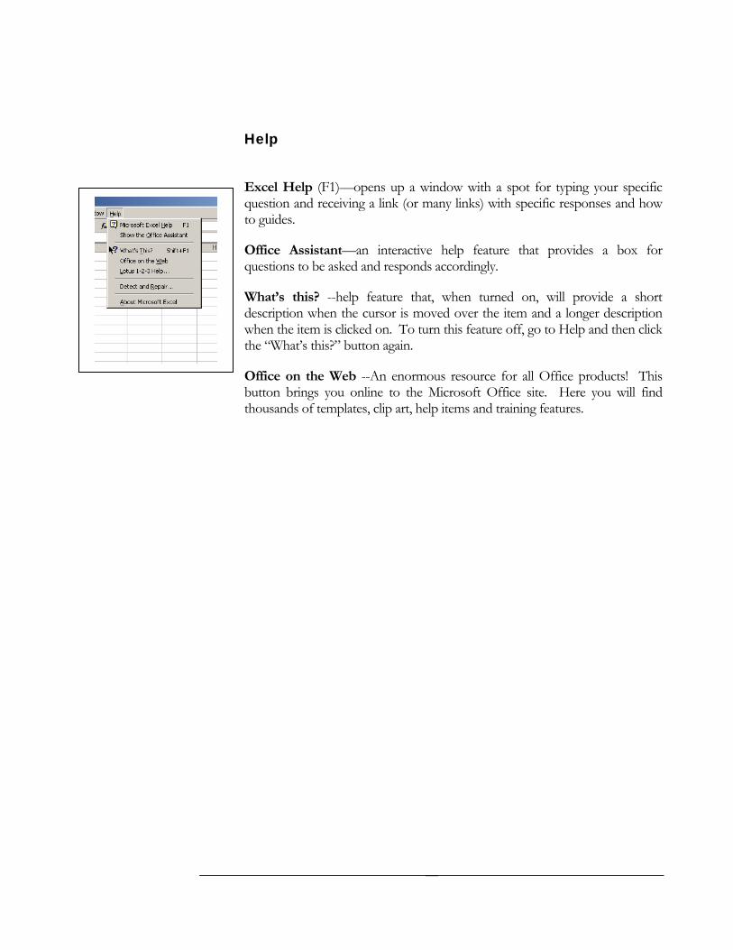
Help
Excel Help (F1)—opens up a window with a spot for typing your specific question and receiving a link (or many links) with specific responses and how to guides.
Office Assistant—an interactive help feature that provides a box for questions to be asked and responds accordingly.
What’s this? --help feature that, when turned on, will provide a short description when the cursor is moved over the item and a longer description when the item is clicked on. To turn this feature off, go to Help and then click the “What’s this?” button again.
Office on the Web --An enormous resource for all Office products! This button brings you online to the Microsoft Office site. Here you will find thousands of templates, clip art, help items and training features.
Updated 9/6/2007
18

Formulas Using the Formula bar To turn on the formula bar, click on View, and then check Formula Bar.
To write a formula using the formula bar:
1. Click in the cell where you want to put the formula
2. On the formula bar, click the equal sign
3. Click on the drop down arrow to the left of the equal sign and select the type of formula you want to use. (sum, product, average, count,…)
4. Once you click on the type of formula you are using, another field appears asking for information regarding that formula type. The example on the right shows the required information for a sum type of formula. You have the option of entering the cell name (ex: B4) or clicking on the button to the right of the text box and clicking on the specified cell.
5. Click the OK button to finish and have the formula added to your spreadsheet. If you do not like the results or change your mind about the formula type, click cancel and start over.
Updated 9/6/2007
19

Lesson 7 Objectives In this lesson, you will write many basic formulas used in spreadsheets.
For each formula, you will use the formula toolbar. To do this, click on
the equal sign below the toolbars. A formula type will appear with a
drop down arrow. Click on the drop down arrow, then More
Functions… to get started.
Writing Basic Formulas 1. Date and Time
a. Click on cell A1
b. Select the function category: Date & Time
c. Select the function name: Today and press OK; the current date will
always be updated into this cell.
2. Math
a. Product (multiplies the numbers in a series)
i. Click on cell F4
ii. Press the equal sign
iii. Select the function category: Math & Trig
iv. Select the function name: Product and press OK
v. Type B4:E4 in the Number 1 box and press OK
b. Sum (adds the numbers in a series)
i. Click on cell F3
ii. Press the equal sign
iii. Select the function category: Math & Trig
iv. Select the function name: Sum and press OK
v. Type B3:E3 in the Number 1 box and press OK
vi. Click on Cell F3, drag the bottom right corner down to cell
F10. You have now made the sum formula occur in each of
the cells in the F column.
Updated 9/6/2007
20

3. Statistical
a. Average (calculates the average of a series)
i. Click on cell F1 and type the title Average
ii. Click on cell F2
iii. Press the equal sign
iv. Select the function category: Statistical
v. Select the function name: Average and press OK
vi. Click cell F2 and drag the box at the bottom right of the cell
down to cell F11. This copies the formula down so you
don’t have to keep typing it over and over.
b. Max (returns the largest number in a series)
i. Click on cell G11
ii. Press the equal sign
iii. Select the function category: Statistical
iv. Select the function name: Max and press OK
v. Type F3:F11 in the box and press OK
4. Linking Cells and Sheets
a. Press the tab for the Averages Sheet and click on cell A1. Press the
= sign on the keyboard. Press the tab for Reg Info and click on Cell
A2. Press enter. You should see that the information from Reg Info
Cell A2 is now in cell A1 of the Average sheet.
b. Click on cell A1 and drag down to cell A9—again you have copied
the formula down to all the cells.
c. Now copy the Averages. First, click on cell B1, press =, click on
the tab Reg Info, click on cell F1 and press enter. Drag the small
box in the lower right corner of cell F1 down to cell F9 so that the
formula copies down.
Updated 9/6/2007
21

5. Logical
a. If (performs a function IF certain conditions exist)
i. Click on cell C1 in the Averages worksheet.
ii. Press the equal sign
iii. Select the function category: Logical
iv. Select the function name: IF and press OK
v. In the top box type: C2>2000 (means if the value of cell C2
is greater than 2000)
vi. In the middle box type: “Over Budget” Note: You must type
the quotation marks if you are using text.
vii. In the bottom box type: “Under Budget” and press OK
Updated 9/6/2007
22

Writing Basic Formulas If you know the formula, you do not have to use the formula bar. To enter a formula without the formula bar, just type:
Function Formula What it Does
=sum(A1:A5) Finds the sum of the data in cells A1 through A5.
=sum(A1,A5) Finds the sum of the data in cell A1 and A5. Sum
=sum(A1:A5,B2) Finds the sum of the data in cells A1 through A5 AND cell B2.
=average(A1:A5) Finds the average of the data in cells A1 through A5.
=average(A1,A5) Finds the average of the data in cells A1 and A5. Average
=average(A1:A5,B2) Finds the average of the data in cells A1 through A5 AND cell B2.
If =IF(B3>C3,"Over
Budget","OK")
If the number in cell B3 is greater than the number in cell C3, then put the word “Over
Budget”, otherwise put the word “OK”.
Count =count(A1:A5) Counts the number of entries in cells A1 through A5. (Each entry counts as 1, so if each of the five
cells has an entry, the answer will be 5.)
Maximum =max(A1:A5) Identifies the largest value in the group of cells from A1 through A5.
Minimum =min(A1:A5) Identifies the smallest value in the group of cells from A1 through A5.
Today’s Date
=today() Enters today’s date into the worksheet.
**Note: Do not put any spaces into your formulas or you will get an error message!
Updated 9/6/2007
23

Formatting Your Worksheet/Workbook Now that you have put your project together, you want to make sure that it formatted so that it is easy to read and use.
Adding color to the text or worksheet
How to Add Colors Select the area you want
to format: Click Format, Cells To change the font, click on the font tab and make adjustments to the size, style, or color.
To change the look of the cell, click on patterns and then select the color and/or shading options
Without color
With color
Tip: You can also select the cells and click Format, AutoFormat to see choices based on preset formatting options.
Printing specific rows or columns on each page
To do this: 1. Click on File, page
setup. 2. Click the tab titled
“Sheet” 3. Click the icon next
to the text box for rows to repeat at top or columns to repeat at left (or both).
4. Click OK
Fitting to one page Click on File, page setup.
Click the tab titled “page”
Under the section called Scaling, select “fit to page” and enter the number of pages wide by the number of pages tall.
Updated 9/6/2007
24

Charting your Data A Step by Step Guide
Step 1 Select the data you want included in your chart.
Step 2 Select Insert, Chart and select the type of chart you want displayed. Note: you can view the chart with your data by clicking View Sample Report
Step 3 Make sure all of your data is selected; if not, click on the icon next to the data range and select the data to include.
Updated 9/6/2007
25

Step 4 Type in the chart title, X-Axis (horizontal) and Y-Axis (vertical) labels.
Step 5: Where do you want your chart?
• Place your chart as an object in your current worksheet
-or- • Create a new sheet—type
the name that you want to name the new sheet.
Updated 9/6/2007
26

Lesson 8 Objectives: Insert a chart of the data
Determine the type of chart to use based upon the data type
Verify that the data range is correct for the chart
Enter the chart title
Enter the x-axis (horizontal) title
Enter the Y-axis (vertical) title
Place a chart in the worksheet or in a new sheet
Charting Your Data 1. Click Insert, Chart
2. Select the type of chart best suited for your data. See the description of
Chart Types located at the back of this Excel Project Book.
3. When you are prompted to enter your data range, use your mouse to
highlight all the cells that contain your data. In this case, you should
hightlight cells A1 through B11. Press Next.
4. Now you are prompted to enter information for your chart settings.
Enter the following:
Chart Title: Average Registrations X-Axis: Type of Vehicle Y-Axis: Number Registered
5. Now you must decide if you want your chart in a sheet of it’s own or
embedded in the worksheet containing the data. For this exercise you will
create a new sheet called Averages Chart by typing the title “Averages
Chart” over the words Chart1.
6. Press Finish and your chart is done.
Updated 9/6/2007
27

Chart Types and Examples
Area C
hart
An area chart emphasizes the magnitude of change
over time. By displaying the sum of the plotted
values, an area chart also shows the relationship of
parts to a whole. Passenger
VehicleStation
WagonCommercial
Farm TruckRecreational
TrailerMotorcycle
Other
Average # Registered
0
50,000
100,000
150,000
200,000
250,000
300,000
350,000
400,000
Average # Registered
Average # Registered
Colum
n Chart
A column chart shows data changes over a period of time or illustrates comparisons among items. Categories are organized horizontally, values vertically, to emphasize variation over time.
0
50,000
100,000
150,000
200,000
250,000
300,000
350,000
400,000
450,000
Average # Registered
Passenger Vehicle
Station Wagon
Commercial
Farm Truck
Recreational
Trailer
Motorcycle
Other
Bar C
hart
A bar chart illustrates comparisons among individual items. Categories are organized vertically, values horizontally, to focus on comparing values and to place less emphasis on time.
Average # Registered
0 200,000
400,000
600,000
Passe
nger
Vehicl
eCommerc
ialRecrea
tiona
lMotorcy
cleAverage # Registered
Line Chart
A line chart shows trends in data at equal intervals.
A v e ra g e # R e g iste re d
0
1 00,000
2 00,000
3 00,000
4 00,000
5 00,000
A v e ra g e # R e g iste re d
Pie C
hart
A pie chart shows the proportional size of items that make up a data series to the sum of the items. It always shows only one data series and is useful when you want to emphasize a significant element.
Average # Registered
Passenger Vehicle
Station Wagon
Commercial
Farm Truck
Recreational
Trailer
Motorcycle
Other
Doughnut C
hart
Like a pie chart, a doughnut chart shows the relationship of parts to a whole, but it can contain more than one data series. Each ring of the doughnut chart represents a data series.
Average # Registered
Passenger Vehicle
Station Wagon
Commercial
Farm Truck
Recreational
Trailer
Motorcycle
Other
Updated 9/6/2007
28

Keyboard Shortcuts Task Keyboard Shortcut
Insert new worksheet SHIFT+F11
Insert cells CTRL+SHIFT+PLUS SIGN
Select the entire worksheet CTRL+A
Select the entire column CTRL+SPACEBAR
Select the entire row SHIFT+SPACEBAR
Move to the beginning of the worksheet CTRL+HOME
Move to the last cell of the worksheet CTRL+END
Display the help task pane F1
Repeat the last command F4
Create a chart of the data in the current range F11
Remove the cell data and formulas DELETE
Cancel an entry in the cell or Formula Bar ESC
Applies the currency format with two decimal places CTRL+$
Copy CTRL+C
Paste CTRL+V
Save CTRL+S
Print CTRL+P
Updated 9/6/2007
29

Other Helpful Sites Website Title Website Address
Microsoft Office on the Web http://office.microsoft.com
The Excel Forum http://www.Excelforum.com/
Dot XLS Consulting http://www.dotxls.com/
Excel User Portal http://www.Exceluser.com/help/index.htm
Excel Maniacs http://www.Excelmaniacs.com/
Contact Information
Michele Marinucci
Training Administrator
State of Delaware
Office of Management and Budget
Human Resource Management
Statewide Training & Organization Development
821 Silver Lake Boulevard, Suite 201
Dover, DE 19904
(302) 739-1990
Updated 9/6/2007
30

Index
Adding color, 22 Arrange, 16 Auto format, 11 Autocorrect, 13 Average, 21 Cell, 2 Cells, 9, 11 Chart, 9 Clear, 5 Close, 3 Column, 2, 9, 11 Comment, 9 Comments, 7 Copy, 5 Count, 21 Customize, 13 Cut, 5 Data, 15 Delete, 5 Delete sheet, 5 Edit, 5 Excel Help, 17 Excel Screen, 2 File, 3 Fill, 5 Filter, 15 Find, 5 Fitting to one page, 22 Footer, 7 Format, 11 Formatting, 22 Formula, 2 Formula bar, 18 Formula Bar, 7 Formulas, 18 Freeze panes, 16 Header, 7 Help, 17 Helpful Sites, 28 Hide, 16 Hyperlink, 9 If, 21 Insert, 9, 11 Keyboard Shortcuts, 27
Maximum, 21 Menu bar, 2 Menu Bar, 3 Minimum, 21 Move/copy sheet, 5 New, 3, 16 Normal View, 7 Office Assistant, 17 Office on the Web, 17 Open, 3 Options, 13 Page break Preview, 7 Page setup, 3 Paste, 5 Picture, 9 Print area, 3 Print preview, 3 Printing, 22 Protection, 13 Repeat, 5 Replace, 5 Row, 2, 11 Rows, 9 Save, 3 Save as, 3 Sort, 15 Spelling, 13 Split, 16 Style, 11 Sum, 21 terms, 2 Today’s Date, 21 Toolbar, 2 Toolbars, 7 Tools, 13 Undo, 5 View, 7 What’s this?, 17 Window, 16 Workbook, 2 Worksheet, 2, 9 Writing Basic Formulas, 21 Zoom, 7
Updated 9/6/2007
31