Microsoft Excel Bootcamp - wisdify.com · Microsoft Excel® Bootcamp 3 COURSE INFORMATION About...

Coughran | Coughran

Microsoft Excel®

Bootcamp

Microsoft Excel® Bootcamp

2

Copyright © 2017 by Wisdify Inc. All rights reserved

This book includes the full text of “Microsoft Excel® Bootcamp”, written by Nathaniel T.

Coughran and Maryn N. Coughran.

No part of this publication may be reproduced, stored in a retrieval system, or transmitted in

any form or by any mean, electronic, mechanical, photocopying, recording, scanning, or

otherwise, except as permitted under Section 107 or 108 of the 1976 United States Copyright

Act, without the prior written permission of Wisdify Inc.

Printed in the United States of America

Wisdify Inc.

464 Common Street, Suite 304

Belmont, MA 02478

www.Wisdify.com


3

COURSE INFORMATION About this course: Microsoft Excel Bootcamp is an online course that can be found at

www.wisdify.com. The online course consists of videos, workbooks, quizzes, and the final exam. This workbook is to be used as a supplement to the online course. Key terms and

definitions cannot be found on the videos but are found in this supplement. Learning Objectives:

• Identify the proper font coloring for a cell containing a formula or an item that should not be modified.

• Recognize the keyboard shortcuts which undoes an action, prints a worksheet, cuts a range, and selects an entire row.

• Identify which keystrokes are required to access the commands on the Quick Access

Toolbar. • Recognize which keystrokes to use to add a new column.

• Recognize which keystrokes to use to change the font size. • Identify an example of a proper use of an absolute cell reference. • Identify and use a formula that sums a range of cells based on some criteria.

• Identify and use a formula that counts the number of cells that meets some criteria. • Identify an example of a proper use of a VLOOKUP formula.

• Identify an example of a proper use of a nested IF statement formula. • Identify a way to work with dates in order to facilitate summarizing data using SUMIFS

and PivotTables.

• Identify an example of a proper use of a MONTH formula. • Identify a function that removes the leading spaces in a text string.

• Determine which tab on the Ribbon contains the Remove Duplicates and Text-to-Columns functions.

• Determine the process to apply Conditional Formatting to a range. • Determine the characteristic required in your source data to create a PivotTable. • Determine the process to insert a Slicer

• Recognize the importance of refreshing a PivotTable when the source data is changed.

Subject Area: Computer Software & App Prerequisites: Participants should have a basic understanding of Excel including how to use

basic functions like SUM and COUNT(A).

Program Level: Basic Advance Preparation: None

Recommended CPE Credit: 4.5 hours


4

Contents

Pt. I: FORMATTING & KEYBOARD SHORTCUTS ................................................................... 6

Formatting Our Data ........................................................................................................................... 6

Font Coloring .............................................................................................................................................................. 6

Number Formatting ................................................................................................................................................... 6

Calculations ................................................................................................................................................................ 6

Fill Colors .................................................................................................................................................................... 7

Keyboard Shortcuts .............................................................................................................................. 7

The Basics ................................................................................................................................................................... 7

The Alt Key ................................................................................................................................................................. 9

Working with Auto Fill ............................................................................................................................................... 9

Customize the Quick Access Toolbar ................................................................................................... 10

Pt. II: FORMULAS BOOTCAMP (pt. I and pt. II) ................................................................. 13

Absolute Cell References .................................................................................................................... 13

Conditional and Lookup Formulas ...................................................................................................... 13

SUMIFS ..................................................................................................................................................................... 13

COUNTIFS ................................................................................................................................................................. 14

VLOOKUP Formula ................................................................................................................................................... 14

IF Formula ................................................................................................................................................................ 16

Nested IF Statements ............................................................................................................................................... 17

Date Functions ................................................................................................................................... 18

Online Topic Videos: EDATE and EOMONTH; YEAR, MONTH, and DAY ................................................................... 18

EDATE ....................................................................................................................................................................... 18

EOMONTH ................................................................................................................................................................ 18

YEAR ......................................................................................................................................................................... 19

MONTH .................................................................................................................................................................... 19

DAY ........................................................................................................................................................................... 19

Text Functions ................................................................................................................................... 19

RIGHT / LEFT ............................................................................................................................................................ 19

MID .......................................................................................................................................................................... 20

Pt. III: WORKING WITH YOUR DATA ................................................................................. 22

Text to Columns ................................................................................................................................. 22

Removing Duplicates ......................................................................................................................... 24


5

Conditional Formatting ...................................................................................................................... 25

Highlight Cells Rules ................................................................................................................................................. 25

Top/Bottom Rules .................................................................................................................................................... 26

Data Bars .................................................................................................................................................................. 26

Color Scales .............................................................................................................................................................. 26

Delete Rules ............................................................................................................................................................. 27

Manage Rules........................................................................................................................................................... 27

Pt. IV: PIVOTTABLES AND SLICERS .................................................................................... 29

PivotTables ........................................................................................................................................ 29

Creating a PivotTable ............................................................................................................................................... 29

Number Formatting in a PivotTable ........................................................................................................................ 31

New Tabs ................................................................................................................................................................. 31

Analyze Tab .............................................................................................................................................................. 32

Design Tab ............................................................................................................................................................... 32

Adding Slicers ........................................................................................................................................................... 33

GLOSSARY........................................................................................................................ 35


6

Pt. I: FORMATTING & KEYBOARD SHORTCUTS

Formatting Our Data

Online Lesson: Formatting & Keyboard Shortcuts

Online Topic Videos: Font coloring and assumptions; Other formatting best practices

Font Coloring

We use different font coloring in our spreadsheet to guide users and tell them how to interact

with our spreadsheet. In general, we use the following 3 basic font coloring:

• BLUE: Indicates that this cell is an input/assumption cell and that the value can

be changed.

• BLACK: Indicates that a cell that should not be modified or overwritten with a

hard-coded value either because it contains a formula or it is a value that will not

change (for example, the historical sales figures).

• RED (optional): Some people like to color cells red that link to other workbooks.

However, this is optional, whereas the blue and black coloring are not.

These font colorings are universal in the Excel world. However, some users are not familiar

with this coloring. Because of this, you can fill in the background of your input/assumptions

cells a light yellow to further indicate that that particular cell can be changed.

Number Formatting

Make sure you format all of your numbers properly! When you leave a number unformatted, it

makes it very hard to read which can lead to errors. Additionally, only add decimal places

when it is absolutely necessary.

Calculations

Don’t ever, ever, ever, ever hard-code in a value into a formula. For instance, this formula is

a big no-no:

=A1*(B1+C1) + 100

Notice that the formula initially references other cells which is perfect. But then, at the end of

the formula, it adds in an arbitrary 100. What does that mean? Why did the person add it

there?

When we hard-code in values in a formula, it can cause 3 major problems:


7

1. It makes the spreadsheet very undynamic. Our entire spreadsheet should be driven by

a few numbers and assumptions. When we hard-code in a number, we then have to

manually go through ever cell that contains that value and change it.

2. It can cause major errors. Many people forget they hard-code in values. This can lead

to major errors down the road as people copy and paste formulas or carrying them into

the future. They are hidden bombs in your spreadsheet

3. It makes it very hard to understand your assumptions. When you hard-code in a value,

you hide from other people your assumptions. This makes it hard to review and audit

your spreadsheet.

Fill Colors

Be very conscience about what fill colors you use. Fill colors should be used to set apart

sections in your spreadsheet. Therefore, only use 2 fill colors max.

Keyboard Shortcuts


Online Topic Videos: Keyboard shortcuts introduction; Basic keyboard shortcuts; Basic

keyboard shortcuts II; The almighty Alt key

The Basics

Keyboard shortcuts can save you immense amounts of time. You may not realize it, but every

time you take your hand off the keyboard to use your mouse, you are wasting precious

seconds. And over the course of a day or week, those seconds turn to minutes which turn to

hours.

Because of that, you NEED to learn keyboard shortcuts. It is more than just a “good to know.”

If you want to master Excel, you need to know keyboard shortcuts.

We have 2 cautions when learning shortcuts:

When you start learning keyboard shortcuts, it WILL be slower than using your mouse. That’s

right. But, you must not quit! Keep at it for a couple weeks and soon the shortcuts will be

muscle memory and automatic. Resist the temptation to go back to your mouse.

If you try to learn every keyboard shortcut, you’ll go nuts! You should learn the shortcuts to

the actions you perform most frequently.

The keyboard shortcuts everyone needs to learn are:

• Copy = Ctrl + C


8

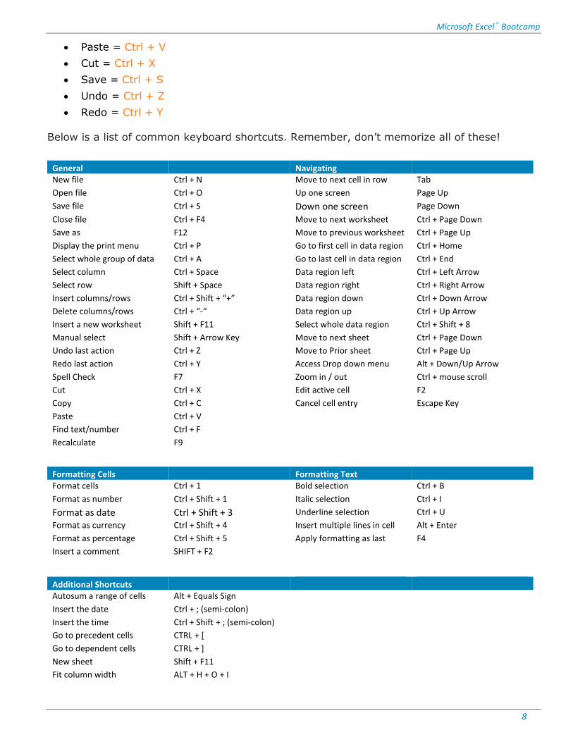
• Paste = Ctrl + V

• Cut = Ctrl + X

• Save = Ctrl + S

• Undo = Ctrl + Z

• Redo = Ctrl + Y

Below is a list of common keyboard shortcuts. Remember, don’t memorize all of these!

Formatting Cells Formatting Text Format cells Ctrl + 1 Bold selection Ctrl + B

Format as number Ctrl + Shift + 1 Italic selection Ctrl + I

Format as date Ctrl + Shift + 3 Underline selection Ctrl + U

Format as currency Ctrl + Shift + 4 Insert multiple lines in cell Alt + Enter

Format as percentage Ctrl + Shift + 5 Apply formatting as last F4

Insert a comment SHIFT + F2

Additional Shortcuts

Autosum a range of cells Alt + Equals Sign

Insert the date Ctrl + ; (semi-colon)

Insert the time Ctrl + Shift + ; (semi-colon)

Go to precedent cells CTRL + [

Go to dependent cells CTRL + ]

New sheet Shift + F11

Fit column width ALT + H + O + I

General Navigating New file Ctrl + N Move to next cell in row Tab

Open file Ctrl + O Up one screen Page Up

Save file Ctrl + S Down one screen Page Down

Close file Ctrl + F4 Move to next worksheet Ctrl + Page Down

Save as F12 Move to previous worksheet Ctrl + Page Up

Display the print menu Ctrl + P Go to first cell in data region Ctrl + Home

Select whole group of data Ctrl + A Go to last cell in data region Ctrl + End

Select column Ctrl + Space Data region left Ctrl + Left Arrow

Select row Shift + Space Data region right Ctrl + Right Arrow

Insert columns/rows Ctrl + Shift + “+” Data region down Ctrl + Down Arrow

Delete columns/rows Ctrl + “-“ Data region up Ctrl + Up Arrow

Insert a new worksheet Shift + F11 Select whole data region Ctrl + Shift + 8

Manual select Shift + Arrow Key Move to next sheet Ctrl + Page Down

Undo last action Ctrl + Z Move to Prior sheet Ctrl + Page Up

Redo last action Ctrl + Y Access Drop down menu Alt + Down/Up Arrow

Spell Check F7 Zoom in / out Ctrl + mouse scroll

Cut Ctrl + X Edit active cell F2

Copy Ctrl + C Cancel cell entry Escape Key

Paste Ctrl + V

Find text/number Ctrl + F

Recalculate F9


9

The Alt Key

Beyond the standard keyboard shortcuts, you can also perform ANY task in Excel using only

your keyboard. The trick is using the Alt key. If you hit the Alt key, letters will appear on the Ribbon.

If you type any of these letters, you will be taken to that tab where more letters will appear. For instance, if you type H after hitting Alt, these new options will appear.

If you now type in A+L, your text in the current cell will become left aligned. So, the

keyboard shortcut to left align your text is: Alt + H + A+L.

Working with Auto Fill Auto Fill allows you to quickly fill cells with data that follow a pattern (ex. months) or that is

based on data in other cells (ex. formulas). For instance, you can automatically populate a sequence of numbers or copy formulas down columns or across rows.

To do this, select the cells that you are using as your starter cells. Click the little box at the bottom right of the cell (your cursor will turn into a cross) and drag it down to fill in the rest

of the series.


10

You can also use Auto Fill to quickly copy a formula down a column by double-clicking the box

at the bottom right of the cell after creating your formula.

Customize the Quick Access Toolbar


Online Topic Videos: Customizing the Quick Access Toolbar

The Quick Access Toolbar is located at the top of your Excel workbook, above the Ribbon. It

provides quick access to your favorite Excel actions. The default functions are Save, Undo, and Redo.

You can customize this to include your favorite actions to save you vast amounts of time:

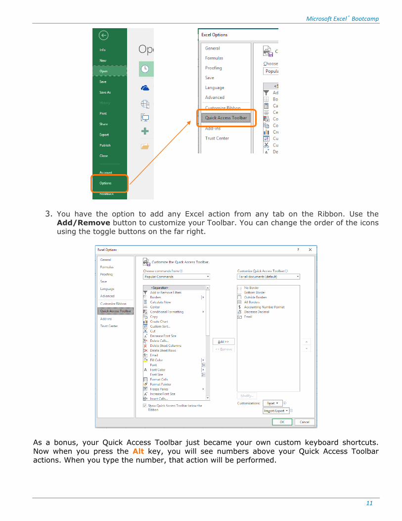
1. Go to the File tab and click on Options (located in the left-hand column). A new window will appear.

2. On the left-hand column, click Quick Access Toolbar.


11

3. You have the option to add any Excel action from any tab on the Ribbon. Use the Add/Remove button to customize your Toolbar. You can change the order of the icons using the toggle buttons on the far right.

As a bonus, your Quick Access Toolbar just became your own custom keyboard shortcuts.

Now when you press the Alt key, you will see numbers above your Quick Access Toolbar actions. When you type the number, that action will be performed.


12

To maximize the utility of your Toolbar, we suggest you place the Toolbar below the Ribbon

for ease of access. You can do this by checking the box labeled Show Quick Access Toolbar

below the Ribbon at the bottom of the menu noted above.


13

Pt. II: FORMULAS BOOTCAMP (pt. I and pt. II)

Absolute Cell References

Online Lesson: Formula Bootcamp pt. I

Online Topic Videos: Absolute cell references

There may be times when you do not want a cell reference to change when copying cells

down a column or across a row. By default, all cells are Relative References. This means that as you copy a formula, the cell references will change based on where you paste the formula. Absolute References on the other hand, do not change when copied. Therefore,

you use an absolute reference to keep a cell, range, or row/column constant.

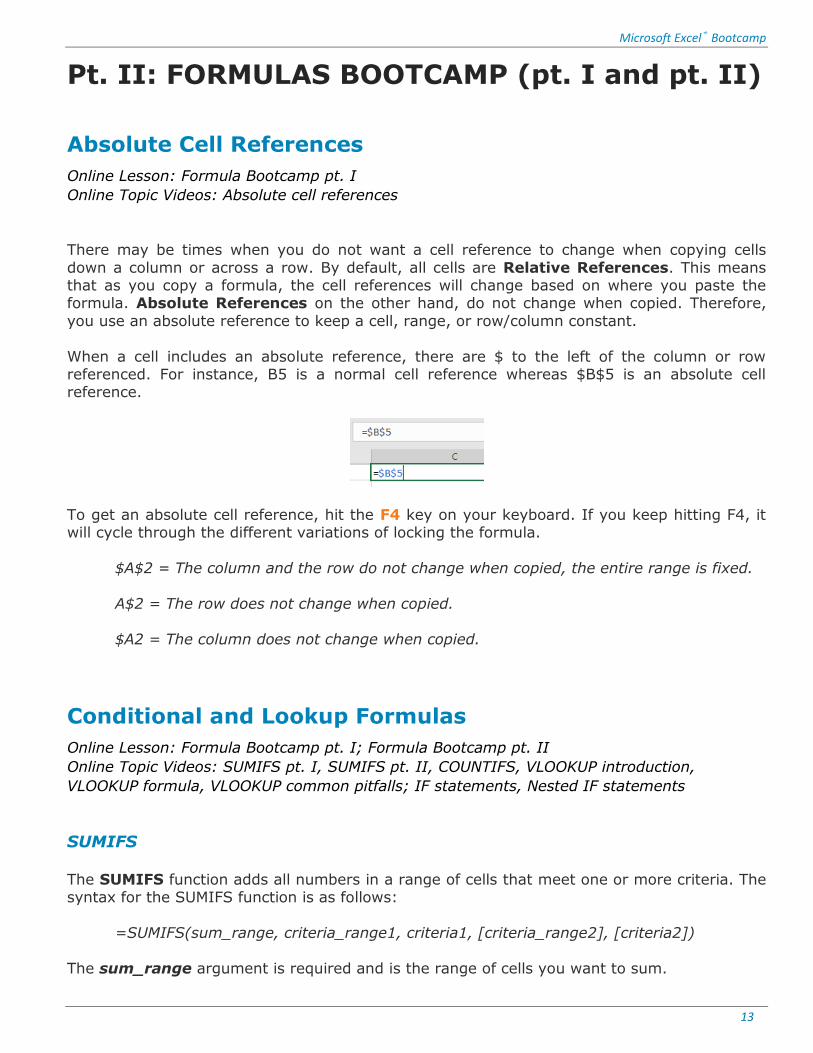
When a cell includes an absolute reference, there are $ to the left of the column or row referenced. For instance, B5 is a normal cell reference whereas $B$5 is an absolute cell reference.

To get an absolute cell reference, hit the F4 key on your keyboard. If you keep hitting F4, it will cycle through the different variations of locking the formula.

$A$2 = The column and the row do not change when copied, the entire range is fixed.

A$2 = The row does not change when copied.

$A2 = The column does not change when copied.

Conditional and Lookup Formulas

Online Lesson: Formula Bootcamp pt. I; Formula Bootcamp pt. II

Online Topic Videos: SUMIFS pt. I, SUMIFS pt. II, COUNTIFS, VLOOKUP introduction,

VLOOKUP formula, VLOOKUP common pitfalls; IF statements, Nested IF statements

SUMIFS

The SUMIFS function adds all numbers in a range of cells that meet one or more criteria. The syntax for the SUMIFS function is as follows:

=SUMIFS(sum_range, criteria_range1, criteria1, [criteria_range2], [criteria2])

The sum_range argument is required and is the range of cells you want to sum.


14

The criteria_range1 argument is required and is the range of cells that you want to apply criteria1 against.

The criteria1 argument is required and is the criteria used to determine which cells to add.

You can add additional criteria and criteria ranges in the subsequent arguments. In the example below, you can add the total number of cars (criteria 1) that Adam (criteria 2)

sold using the formula:

=SUMIFS(A2:A6, B2:B6, “Car”, C2:C6, “Adam”) which returns the value 6

COUNTIFS

The COUNTIFS function counts the number of cells in a range that meets one or more criteria. The syntax for the COUNTIFS function is as follows:

=COUNTIFS(criteria_range1, criteria1, [criteria_range2], [criteria2], ...)

The criteria_range1 argument is required and is the range of cells that you want to test criteria1 against.

The criteria1 argument is the criteria used to determine which cells to count. You can add additional criteria and criteria ranges in the subsequent arguments.

In the example below, you can count the total number of times Adam (criteria 1) received a

passing grade (criteria 2) using the formula: =COUNTIFS(A2:A6, “Adam”, C2:C6, “Y”) which returns the value 2

VLOOKUP Formula

The VLOOKUP function searches vertically (top to bottom) the leftmost column of a lookup

table until it locates a value that matches or exceeds the one you are looking up. Think of the


15

VLOOKUP as a phone book. You want to look up a person’s phone number so you open the phone book, look up their last name, and then go over and find their number. The VLOOKUP

does the exact same thing.

The VLOOKUP function uses the following syntax: =VLOOKUP(lookup_value, table_array, col_index_num, [range_lookup])

The lookup_value argument is the value that you want to look up in the first column of the

lookup table (for example you want to lookup “Gimli”). The table_array is the lookup table’s cell range. This is the entire table (i.e. phone book).

In the example below, cell B7 has the lookup_value (Gimli) and cells A2:C5 is the table_array (the phone book where we want to look up Gimli).

The col_index_num argument is the column number in the table from which the matching value must be returned. The first column is 1. In the above example, Name is column 1, Age is column 2, and Gender is column 3.

The not-so-optional range_lookup argument is either TRUE or FALSE. This tells Excel

whether you want Excel to find an exact (FALSE) or approximate (TRUE) match. When you specify TRUE or omit the range_lookup argument, Excel finds an approximate match. When you specify FALSE as the range_lookup argument, Excel finds only exact matches. Unless it is

a special situation, you should put FALSE 99% of the time.

The reason is, if your lookup values (Name in our example), is not in alphabetical or numerical order and you do not choose the FALSE option, the VLOOKUP will not return accurate results.

Putting this together, the formula =VLOOKUP(A1,C2:E5, 2, FALSE) will return Gimli’s age

which is 140.


16

IF Formula

The IF function will return a value based on whether a given condition is TRUE or FALSE. It is a simple IF, THEN, ELSE operation.

For example, IF cell A1 is greater than B1, THEN you want C1 to show “Original”. ELSE if it is not true, you want C1 to show “Duplicate”.

The IF function uses the following syntax:

=IF (logical_test, value_if_true, value_if_false)

The logical_test argument is required and is the condition you want to test. To test a condition, you need to use a comparison operator:

• Greater than (>)

• Greater than or equal to (>=)

• Less than (<)

• Less than or equal to (<=)

• Equal to (=)

• Not equal to (<>).

For example, if you want to test whether cell A1 is larger than B1, you would put A1>B1. You are not limited to testing cell references. You can test fixed numbers (A2>10) or text strings (A2= “John Doe”).

The value_if_true argument is required and is the value or text that will appear if the logical

test is true.

For instance, if A1 is greater than B1 you can have the cell return the text “Original”. You can also have the formula return a fixed value (10) or a formula (D2*E2).

The value_if_false argument is required and is value or text that will appear if your test is false (i.e. A2 is NOT larger than B2). Once again, the formula can return text, a fixed value,

or a formula. In our example, we’ll put “Old Property”. Let’s use an example. Let’s suppose on a test, the teacher had an extra credit question.

However, she stipulates that you can only get the extra credit if you missed less than 2 days of class. If you missed 2+ days of class, you would not get the extra credit.


17

The calculate this in column D, we would use the formula:

=IF(C3<2, A2+B2, A2)

You can have the IF statement return a blank cell by putting two quotation marks (“”) in the

value_if_true or value_if_false part of the formula.

Nested IF Statements

You can nest multiple (up to 7) IF statements into a single formula. But truth be told, if you

have more than 2 or three nests, there is probably a better formula. Nested IF statements are helpful if you need two or more conditions to be met.

Let’s say you need to test whether something is Okay, Bad, or Very Bad. A nested IF statement would look like this:

=IF(A1>0, “Okay”, IF (A1<-1000, “Very Bad”, “Bad”))

Let’s break down the parts:

=IF(A1>=0, “Okay”: If cell A1 is greater than zero, then put “Okay” in the cell.

, IF (D3<-1000, “Very Bad”: This is where the nest begins. If the first statement is false, then you want to test another assumption. In this case, you now want to see if A1 is less than

($1,000). If so, then put “Very Bad”. ,” Bad”): Finally, if the first and second statements are false, then put “Bad”. In other words,

if A1 falls between ($1) and ($999).

Nested IF statements are easy once you understand the general concept. Another way to look at nested statements is like this: =IF This statement is true, then return this value, otherwise IF (This statement is true, then


18

return this value, otherwise return this value)).

Date Functions

Online Lesson: Formula Bootcamp pt. II

Online Topic Videos: EDATE and EOMONTH; YEAR, MONTH, and DAY

EDATE

The EDATE (for Elapsed Date) function calculates a future or past date that is x number of

many months ahead or behind the date that you specify as its start_date. You can use the EDATE function to quickly determine the particular date at a particular interval in the future or

past (for example, three months ahead or one month ago).

The EDATE function has the following syntax: =EDATE(start_date, months)

The start_date argument is the date that you want to use as the beginning date.

The months argument is a positive (for future dates) or negative (for past dates) integer that represents the number of months ahead or months past to calculate.

For example, suppose cell A1 has the date 1/15/2018. When you enter the following EDATE

function in cell B1:

=EDATE(A1,1)

Then Excel would return the date 2/15/18.

EOMONTH

The EOMONTH (for End of Month) function calculates the last day of the month that is x number of months ahead or behind the date that you specify as its start_date. You can use

the EOMONTH function to quickly determine the end of the month at a set interval in the future or past.

The syntax on EOMONTH is the same as EDATE.

For example, suppose cell A1 has the date 1/15/18 and you enter the following EOMONTH function in cell B1:

=EOMONTH(A1,1)

Then Excel would return the date 2/28/18.


19

YEAR

The YEAR function returns the year of a specified date.

For example, suppose cell A1 has the date 1/15/18 and you enter the following YEAR function

in cell B1:

=YEAR(A1)

Excel would return the year 2018 in cell B1.

MONTH

The MONTH function returns the month (as a number) of a specified date.

For example, suppose cell A1 has the date 1/15/18 and you enter the following MONTH

function in cell B1:

=MONTH(A1)

Excel would return the number 1 (i.e. month 1) in cell B1.

DAY

The DAY function returns the day of a specified date.

For example, suppose cell A1 has the date 1/15/18 and you enter the following DAY function

in cell B1:

=DAY(A1)

Excel returns the day 15 in cell B1.

Text Functions

Online Lesson: Formula Bootcamp pt. II

Online Topic Videos: LEFT, RIGHT, and MID; TRIM

RIGHT / LEFT

The RIGHT function returns the last character(s) in a text string, based on the number of

characters you specify, while the LEFT function returns the first character(s) in a text string.


20

The syntax for both function is as follows:

=RIGHT(text, [number_of_characters])

=LEFT(text, [number_of_characters]) The text argument is the string that you wish to extract from.

The number_of_characters argument is the number of characters that you wish to extract

starting from the right-most character (RIGHT function) or left-most character (LEFT function).

Let’s assume that cell A1 contains the text “Guacamole”. The RIGHT and LEFT formulas below would return the following:

=RIGHT(A1, 4) would return “mole”

=LEFT(A1, 4) would return “Guac”

MID

The MID function is similar to the RIGHT/LEFT functions except it returns the middle

character(s) in a text string based on the number of characters you specify.

The MID syntax is as follows:

=MID(text, start_num, num_chars) The text argument is the text you want to extract from.

The start_num argument is the location of the first character to extract.

The num_chars argument is the number of characters to extract.

For example, if you have the text “The Quick Brown Fox” in cell A1 and wanted to extract “Quick”, you would use the following formula:

=MID(A1,5,6)

You use 5 as the start_num since “Q” is the 5th character in the string (spaces count as a character). You use 6 as the num_chars since there are six characters in the word “Quick”.


21


22

Pt. III: WORKING WITH YOUR DATA

Text to Columns

Online Lesson: Working with Data & Conditional Formatting

Online Topic Videos: Text-to-Columns

Text to Columns (found on the Data tab on the Ribbon) can be used to separate data that

is contained in single column into multiple columns.

For example, if your raw data dump puts the employee’s last name, first name, and ID

number all in one cell, you can use Text to Columns to separate the data.

Select the cells that contains the text you want to separate and then click the Text to

Columns command. A wizard dialog box will open to help you through the process.

In step 1 of the wizard, select whether the text is Delimited or Fixed Width. Delimited text is text that has some character, such as a comma, tab, or space, separating each group of words that you want placed into its own column. Fixed-width text describes text where each

group is a set number of characters. We’ll only walk through Delimited as that is the most common. After selecting the data type, click Next.


23

In the next screen, you will provide details on how you want the text separated. Check the boxes that describe how your text is separated. In our example, the text is separated by a

comma. You will note that under Data preview you can see how Excel will separate your data before you finish. Once it is separated as desired, click Next.

In the final step, you will tell Excel where you want to place the separated text under Destination. Once you have selected the destination, click Finish.


24

Removing Duplicates


Online Topic Videos: Remove duplicates

If you have a list of data that potentially have duplicate information, you can use Remove

Duplicates to quickly get rid of the extra data. Remove Duplicates is found on the Data tab.

To remove the duplicate values, first select the entire data set you want to analyze, including

header rows, and click the Remove Duplicates button on the Data tab. The following menu will appear.

On the form under Columns, there are checkboxes next to each of the headers (“Acct Number” and “Balance” in our example). The more boxes you check, the more precise the

removal will be.

For examples, by checking off both the “Acct Number” and “Balance” boxes, Excel will only remove rows that are both duplicative in terms of the account number and account balance. If you only check off the “Acct Number” checkbox, Excel will remove all rows that just have

duplicative account numbers even if the account balance is different.

We highly recommend keeping all boxes checked. After you are done, click OK. A message box will appear indicating how many duplicates were found and removed, and how many values remain.


25

Conditional Formatting


Online Topic Videos: Conditional Formatting pt. I, Conditional Formatting pt. II, Conditional

Formatting pt. III

Conditional Formatting allows you to automatically change the formatting of cells based on

criteria you set. For instance, you can have all cells that are over a certain threshold be

highlighted in yellow.

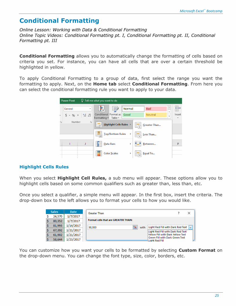
To apply Conditional Formatting to a group of data, first select the range you want the

formatting to apply. Next, on the Home tab select Conditional Formatting. From here you

can select the conditional formatting rule you want to apply to your data.

Highlight Cells Rules

When you select Highlight Cell Rules, a sub menu will appear. These options allow you to

highlight cells based on some common qualifiers such as greater than, less than, etc.

Once you select a qualifier, a simple menu will appear. In the first box, insert the criteria. The

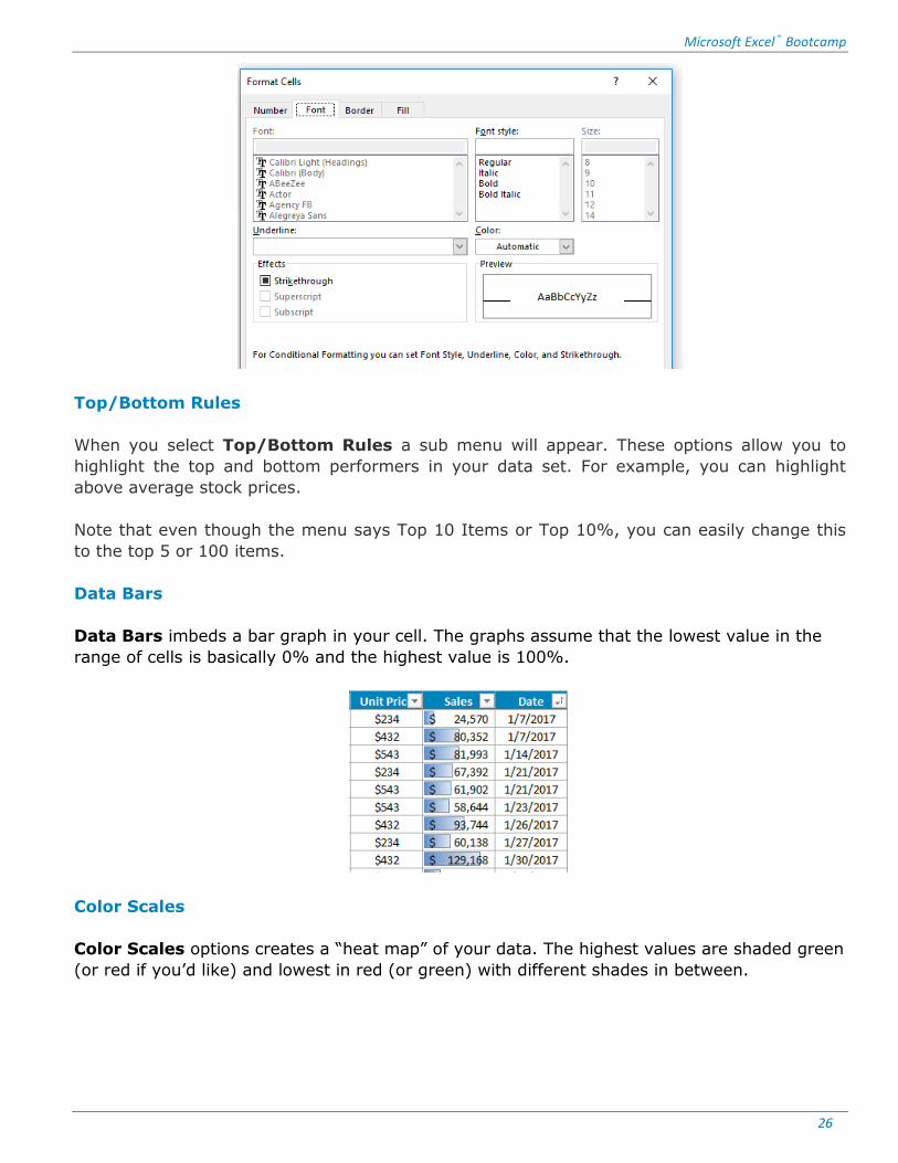
drop-down box to the left allows you to format your cells to how you would like.

You can customize how you want your cells to be formatted by selecting Custom Format on

the drop-down menu. You can change the font type, size, color, borders, etc.


26

Top/Bottom Rules

When you select Top/Bottom Rules a sub menu will appear. These options allow you to

highlight the top and bottom performers in your data set. For example, you can highlight

above average stock prices.

Note that even though the menu says Top 10 Items or Top 10%, you can easily change this

to the top 5 or 100 items.

Data Bars

Data Bars imbeds a bar graph in your cell. The graphs assume that the lowest value in the

range of cells is basically 0% and the highest value is 100%.

Color Scales

Color Scales options creates a “heat map” of your data. The highest values are shaded green

(or red if you’d like) and lowest in red (or green) with different shades in between.


27

Delete Rules

If you need to delete the rules of a particular set of cells, first select the cells you want to

modify. Now, go to Conditional Formatting on Home tab and select Clear Rules. You can

either delete the rules of particular set of cells (that you’ve highlighted) or from the entire

worksheet.

Alternatively, you can go to Manage Rules to delete your formatting.

Manage Rules

If at any time you need to delete a formatting rule, change the data range, or change how

you want the cells to be formatted, you can do this in the Manage Rules section.

First, highlight the range of cells that you want to modify. From there, go to Conditional

Formatting on the Home tab and select Manage Rules.

A menu will appear showing the various rules you have applied to your selection. To delete a


28

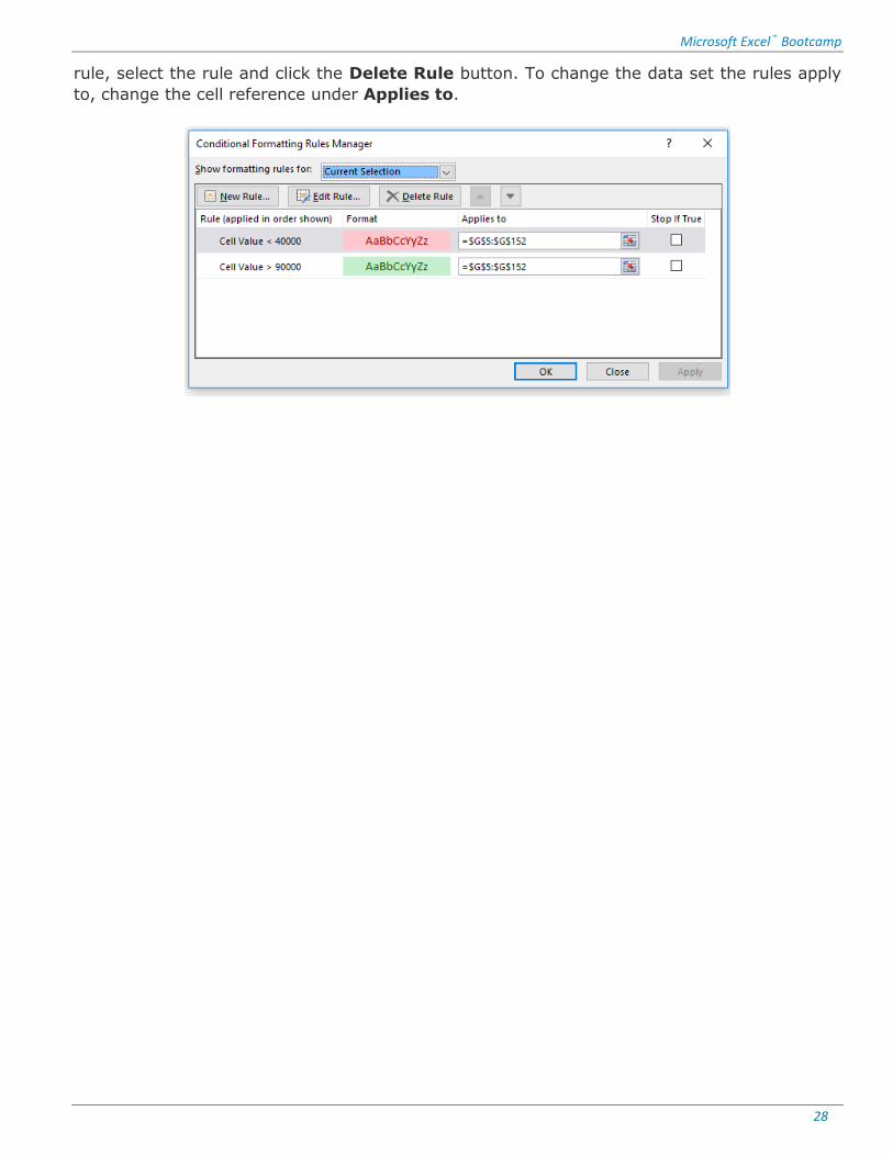
rule, select the rule and click the Delete Rule button. To change the data set the rules apply

to, change the cell reference under Applies to.


29

Pt. IV: PIVOTTABLES AND SLICERS

PivotTables

Online Lesson: PivotTables

Online Topic Videos: Introduction; Drilling into our data; Formatting our PivotTable; Slicers

Creating a PivotTable

The PivotTable function in Excel is one of the most powerful data analyzing tools in Excel.

PivotTables help you automatically summarize, analyze, explore, and present your data with a few clicks. To create a PivotTable:

1. Make sure your data has column headings, that there are not blank rows, and that your data is completely cleaned up (remove all duplicates, all data present, etc.).

2. Click any cell in the range of cells or table.

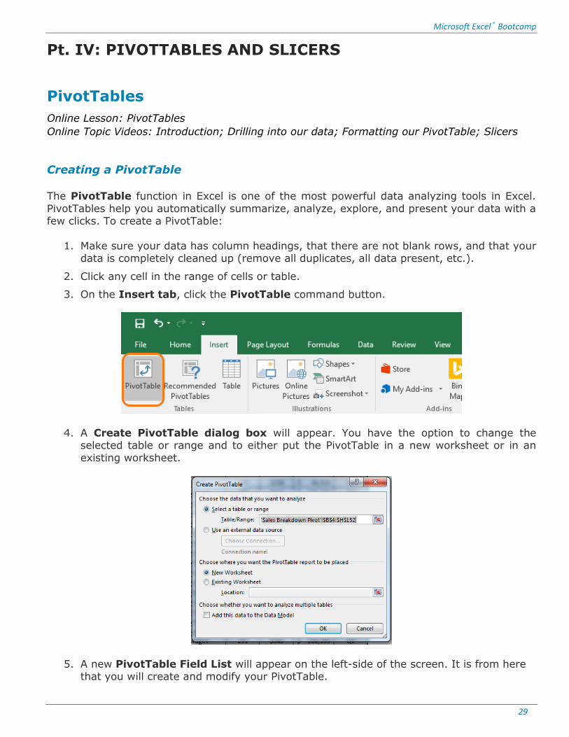
3. On the Insert tab, click the PivotTable command button.

4. A Create PivotTable dialog box will appear. You have the option to change the selected table or range and to either put the PivotTable in a new worksheet or in an

existing worksheet.

5. A new PivotTable Field List will appear on the left-side of the screen. It is from here that you will create and modify your PivotTable.


30

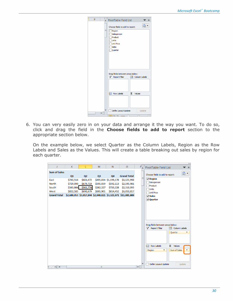
6. You can very easily zero in on your data and arrange it the way you want. To do so,

click and drag the field in the Choose fields to add to report section to the appropriate section below.

On the example below, we select Quarter as the Column Labels, Region as the Row Labels and Sales as the Values. This will create a table breaking out sales by region for

each quarter.


31

7. You can add multiple layers to your PivotTable by dragging fields below or above the Row Labels or Column Labels. However, we recommend you only have one field in

the Column area. Two to Three is the optimal number of fields in the Row area.

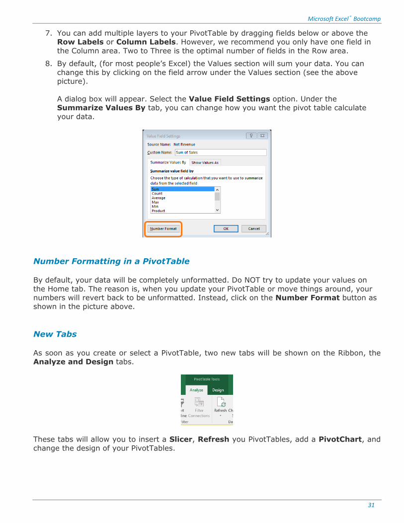
8. By default, (for most people’s Excel) the Values section will sum your data. You can

change this by clicking on the field arrow under the Values section (see the above picture).

A dialog box will appear. Select the Value Field Settings option. Under the Summarize Values By tab, you can change how you want the pivot table calculate

your data.

Number Formatting in a PivotTable

By default, your data will be completely unformatted. Do NOT try to update your values on

the Home tab. The reason is, when you update your PivotTable or move things around, your numbers will revert back to be unformatted. Instead, click on the Number Format button as shown in the picture above.

New Tabs

As soon as you create or select a PivotTable, two new tabs will be shown on the Ribbon, the Analyze and Design tabs.

These tabs will allow you to insert a Slicer, Refresh you PivotTables, add a PivotChart, and

change the design of your PivotTables.


32

Analyze Tab

• Insert Slicer – Slicers are a great way to slice and dice your data. We cover this more

in-depth below.

• Refresh – After you create your pivot table, you may need to change your source data. Unlike a chart that automatically updates after you change your source data, a

PivotTable will not. You must manually refresh your PivotChart every time you update you source data! To update, go to the Analyze tab and click the Refresh command

button.

• Move PivotTable – Move your PivotTable to a new sheet or to an existing sheet.

• Fields, Items, & Sets – You can add a customized Calculated Field to your PivotTable.

We go over this below.

• PivotChart – Create a PivotChart from your PivotTable. We go over then in depth

below.

• Field List / +- Buttons / Field Headers – The Field List button will add or remove the PivotTables Fields box from the right-side of your screen. The Field Headers should

(in our opinion) always be removed by clicking the Field Headers button. This gets rid of the in-PivotTable ability to filter. You should use Slicers instead. Doing this will clean

up your PivotTable.

Design Tab

• Subtotals – Change the position of the subtotals or remove subtotals. We recommend

you always put subtotals as the bottom of a group to make the table easier to read.

• Grand Totals – Add or remove grand totals from your rows and columns.

• Report Layout – We think the default layout is perfect. Feel free to play with these to see different default options.

• Blank Rows – Add a blank row after each line will make your PivotTable easier to

read.

The various check boxes will allow you to change the view of your PivotTable. We think the default settings are perfect so don’t recommend changing this too much. You can


33

You can also change the PivotTable Style to a different color scheme or create your own custom style by clicking on the New PivotTable Style option.

Adding Slicers

In Microsoft Excel 2010 and above, you can use slicers to quickly and easily filter your

PivotTable or PivotChart. In addition to quick filtering, slicers also show you which items are being filtered which makes it easy to understand what exactly is shown in a filtered report.

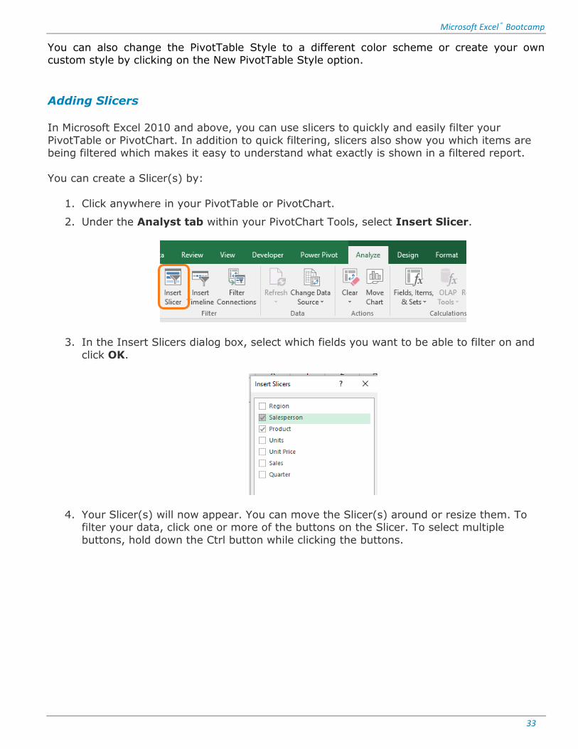
You can create a Slicer(s) by:

1. Click anywhere in your PivotTable or PivotChart.

2. Under the Analyst tab within your PivotChart Tools, select Insert Slicer.

3. In the Insert Slicers dialog box, select which fields you want to be able to filter on and

click OK.

4. Your Slicer(s) will now appear. You can move the Slicer(s) around or resize them. To filter your data, click one or more of the buttons on the Slicer. To select multiple

buttons, hold down the Ctrl button while clicking the buttons.


34

5. You can delete a Slicer by clicking on it and pushing the Delete key on your keyboard.


35

GLOSSARY

Absolute References –

Auto Fill – Allows the users to fill cells with data that follows a pattern or that is based on data in other cells.

Conditional Formatting – Allows a user to automatically apply formatting (such as colors, icons, and data bars) to one or more cells based on a condition being met.

COUNTIFS –A function that counts the number of cells in a range that meets one or more criteria.

DAY – A function that returns the day of a specified date.

EDATE (Elapsed Date) – A function that calculates a future or past date that is x number of many months ahead or behind the date that you specify as its start_date.

EOMONTH (End of Month) – A function that calculates the last day of the month that is x

number of months ahead or behind the date that you specify as its start_date.

IF – A function that will return a value based on whether a given condition is TRUE or FALSE. LEFT – A function that returns the first character(s) in a text string, based on the number of

characters you specify.

MID – A function that is similar to the RIGHT/LEFT functions except it returns the middle character(s) in a text string based on the number of characters you specify.

MONTH – A function that returns the month (as a number) of a specified date.

Nested IF – An IF function that incorporates one or more additional IF functions to test for three or more conditions.

PivotTable – A function in Excel that helps a user summarize, analyze, explore, and present data in a table format.

Quick Access Toolbar – A customizable toolbar that contains a set of commands that are independent of the tab on the ribbon that is currently displayed.

Relative References –

Remove Duplicates – A command found on the Data tab on the Ribbon that allows the user to get rid of duplicate data.

RIGHT – A function that returns the last character(s) in a text string, based on the number of

characters you specify. Slicer – A PivotTable tool that allows a user to quickly filter a PivotTable. Additionally, the

Slicer can show a user which items are being filtered.


36

SUMIFS – A function that adds all numbers in a range of cells that meet one or more criteria.

Text to Columns – A command found on the Data tab on the Ribbon that can be used to separate data that is contained in single column into multiple columns.

VLOOKUP – A function that searches vertically (top to bottom) the leftmost column of a lookup table until it locates a value that matches or exceeds the one you are looking up.

YEAR – A function that returns the year of a specified date.

Microsoft Excel Bootcamp - wisdify.com · Microsoft Excel® Bootcamp 3 COURSE INFORMATION About...

Documents

Transcript of Microsoft Excel Bootcamp - wisdify.com · Microsoft Excel® Bootcamp 3 COURSE INFORMATION About...