Microsoft Excel 2010 – Level 1 Learning Guides... · Microsoft Excel 2010 ... Microsoft Office....

T r a i n i n g G u i d e

Microsoft Excel 2010

– Level 1

1 – Getting to know Microsoft Excel

Microsoft Excel 2010 - Level 1

© Learning and Development Service Getting to know Microsoft Excel

GETTING TO KNOW MICROSOFT EXCEL

Microsoft Excel is a spreadsheet application that is usually part of a suite of Microsoft applications, known as Microsoft Office.

You can use Excel for all sorts of tasks involving numbers such as budgeting, sales analysis, forecasting, charting and graphing and much more. Excel is a tool used to perform calculations with numbers so virtually any task that requires calculation and number crunching can be setup and performed in Excel.

In this booklet you will:

learn how to start Microsoft Excel 2010

gain an understanding of the Microsoft Excel 2010 screen

gain an understanding of how Microsoft Excel 2010 works

learn how to use the Ribbon

learn how to use the keytip badges on the Ribbon

learn how to minimise the Ribbon

gain an understanding of Backstage View in Microsoft Excel

learn how to access the Backstage View

learn how to use shortcut menus

gain an understanding of how dialog boxes work

learn how to launch a dialog box

gain an understanding of the Quick Access Toolbar learn how to add commands to the Quick Access

Toolbar

gain an understanding of the status bar

learn how to exit correctly and safely from Microsoft Excel 2010

INFOCUS



STARTING MICROSOFT EXCEL

Try This Yourself:

Before you begin, ensure that your computer is switched on and that the Windows desktop is displayed on your screen…

1 Click on the Windows Start button (it’s a round button with a Windows logo on it) at the bottom left-hand corner of the screen to display the menu

2 Click on All Programs

3 Click on Microsoft Office

4 Click on Microsoft Excel 2010

After a few moments of huffing and puffing Excel will start with a blank “workbook” on the screen – the workbook appears like an electronic sheet of paper ruled into columns and rows.

For Your Reference… To start Microsoft Excel:

1. Click on the Windows Start button 2. Click on All Programs 3. Click on Microsoft Office 4. Click on Microsoft Excel 2010

Handy to Know… • If you have accessed Microsoft Excel

several times it should appear in the first part of the Start menu – this means you won’t need to continue to the All Programs menu.

To create a new spreadsheet, or edit an existing one, the first thing that you need to do is to start Microsoft Excel. As a standard software application, how Microsoft Excel is started is largely

determined by Windows. For example, it can be started from the Windows Start menu, from a shortcut, or even by opening a workbook (project) that was created previously in Excel.

4

1

2

3



THE EXCEL 2010 SCREEN

1

2

The Microsoft Excel 2010 screen is made up of several key elements. Some of these, such as the Ribbon and the Backstage, are common to other Office 2010 applications so once you know how they

work you won’t have to relearn them when you use other applications. The unique aspect of Excel is the worksheet where you enter and work with your data.

1 The Ribbon is the tabbed band that appears across the top of the window. It is the command control centre of Excel 2010. You use the tabs on the Ribbon to access commands which have been categorised into groups. Commands can be buttons or sometimes include galleries of formatting options that you can select from.

2 The File tab is used to access the Backstage view which contains file management functions such as saving, opening, closing, printing, sharing, etc. Excel Options are also available so that you can set your working preferences and options for Excel 2010.

3 The Worksheet is like an electronic piece of paper ruled into columns and rows. The worksheet is where you type numbers, letters, and formulas to perform calculations. Notice that columns are headed using letters of the alphabet (A, B, C, etc) while rows are designated using numbers down the left side.

4 The Active Cell is where text, numbers, and formulas will appear when you start typing.

5 The Mouse Pointer is used, amongst other things, to select a cell and make it active. It may appear as a large cross, as in this example, as an I-bar, or any number of other forms, depending upon its function at that position on the screen.

6 The Status Bar appears across the bottom of the window and displays useful information about what is happening in the worksheet. At present it shows Ready which means that Excel is ready to be used for your project.

7 The View buttons and the Zoom Slider are used to change the view or to increase/decrease the zoom ratio for your worksheet.

8 The Scroll bar indicates your current position in the worksheet and lets you move to other positions in the worksheet by clicking or dragging. The arrows can also be used to move through the worksheet.

4

5

3

8

6 7



HOW MICROSOFT EXCEL 2010 WORKS

1

For a novice user the Microsoft Excel 2010 screen can seem intimidating. You’ll soon see that it is made up of only three key areas. The data you type is placed on a worksheet. The data within the worksheet

can be manipulated and changed using commands on the Ribbon. The worksheet is part of a larger entity known as a workbook which is controlled on the Backstage.

The Worksheet A worksheet appears as a number of rows and columns which form squares known as cells. Everything you type in Excel is entered into these cells. In the simple business plan shown here there are numbers and words entered into a worksheet. Formulas are also entered that automatically perform calculations. The worksheet is part of a larger entity known as a workbook – workbooks can be filed away for future use or for sharing and can also be printed.

2 The Ribbon When you need to do something with the data on a worksheet, such as format it, colour it, analyse it, move it, copy it, and much more, you’ll find all of the relevant commands on the Ribbon. The Ribbon has commands organised thematically using a series of tabs across the top.

Backstage When you want to do something with the data in your worksheet, such as save it so that you can access it again later, print it, share it with a colleague, send it to your boss, protect it from prying eyes, or whatever, you will need to access the Microsoft Office Backstage area of Microsoft Excel. The Backstage is accessed using the File tab on the Ribbon. Rather than offering you commands on a Ribbon, Backstage occupies the entire screen and has a series of options down the left side. Here the Print option is active, and that is why you can see a preview of the worksheet and a series of print-related options on the right side of the Backstage.

3



USING THE RIBBON

For Your Reference… To use the Ribbon:

1. Click on a tab to display the commands

2. Click on a button to activate a command, display a gallery, or display a dialog box

Handy to Know… • Additional tabs known as Contextual

tabs appear in specific circumstances. For example, if you insert a picture, the Picture Tools: Format tab will appear. This provides quick access to all of the tools you may need to modify and work with the picture.

3

2

The Ribbon is the command centre for Microsoft Excel. It provides a series of commands organised into groups and placed on relevant tabs. Tabs are activated by clicking on their name to

display the command groups. Commands are activated by clicking on a button, tool or gallery option. Everything you could possibly want to do in Excel will be found somewhere on this Ribbon.

Dialog boxes like this one provide settings or options for you to choose from. For example in this one you can zoom the screen by varying percentages. We won’t actually do anything at this point. You’ll get plenty of opportunity for using dialog boxes at a later stage…

5

Try This Yourself:

Before trying this ensure that Microsoft Excel 2010 has started…

1 Examine the groups on the Home tab

These are the most commonly used commands, including copy and paste, font and number formatting, styles and editing...

2 Click on the Insert tab

The commands on this tab are used to create tables, illustrations, charts, headers and footers, text objects and symbols...

3 Click on Shapes in the Illustrations group to display the Shapes gallery

A huge range of shapes will appear which can be inserted into the worksheet…

4 Click on some of the other tabs across the top of the Ribbon (Page Layout, Formulas, etc) and examine the commands on them

Some of these open “dialog boxes”...

7 On the View tab, click on Zoom in the Zoom group to display the Zoom dialog box

8 Click on [Cancel] then click on the Home tab



USING RIBBON KEY TIPS

Try This Yourself:


1 Press to display the key tip badges for the tabs

2 Press to display the Page Layout tab and to see the key tip badges for these commands

3 Press to display the Margins options

Here you could use the or keys to move through the options, or to see Custom Margins…

4 Press twice to return to the Tab level of key tips

5 Press to access the Formulas tab

6 Press five times and notice that Logical is selected

7 Press to see a list of Logical functions, then press several times to move down the menu

8 Press to abort the operation

For Your Reference… To use KeyTip Badges to access commands:

1. Press to display the KeyTip Badges

2. Press the letter key of the command or tab that you want to select

Handy to Know… • You can still use the shortcut keys for

menu commands that were available in previous versions of Office. For example, + applies bold to selected text.

1

2

The Ribbon is normally accessed with a mouse. However you can also use the keyboard to access Ribbon commands. When you press the key on the keyboard alphabetical labels, known as

key tip badges, appear on the Ribbon. Pressing a key on the keyboard will activate the corresponding command on the Ribbon just as if you’d clicked the command with the mouse.

3

6



MINIMISING THE RIBBON

Try This Yourself:


1 Click on the Insert tab to display the Insert commands

2 Double-click on the Insert tab to minimise the ribbon

While the tabs stay visible, the rest of the commands are hidden...

3 Click on the Page Layout tab to temporarily redisplay the ribbon, this time with the Page Layout commands

4 Click anywhere in the worksheet

The ribbon will hide again – it only becomes visible when you need it...

5 Double-click on the Insert tab to redisplay the Ribbon permanently again

6 Click anywhere in the worksheet

This time the ribbon has been redisplayed permanently and doesn’t disappear when you aren’t using it...

For Your Reference… To hide/display the Ribbon:

1. Double-click on the active tab to hide the Ribbon

2. Click on a tab to see the Ribbon temporarily

3. Double-click on a tab to redisplay the Ribbon permanently

Handy to Know… • There are special buttons at the right

of the Ribbon that also control minimising and maximising of the Ribbon. When a Ribbon is in its minimised state a pin button appears which will make the Ribbon large and permanent again.

1

2

The Ribbon at the top of the screen, valuable as it is, does tend to occupy a reasonable amount of space. You can minimise the Ribbon so that only the tabs appear visible. You can minimise the

Ribbon as a once-off operation, or have it remain constantly minimised and display full commands only briefly while a tab has been clicked.

3

5

Look closely here and you’ll see that the Ribbon is actually sitting over the worksheet –you can’t see rows 1 and 2 because they are being obscured by the Ribbon



UNDERSTANDING THE BACKSTAGE VIEW

The Ribbon allows you work on the content in a worksheet – you can add more content, colour it, chart it, analyse it, copy it, and much more. The Backstage, which is accessed using the File tab, allows you

to do something with the content you create. You can save it for reuse later, print it on paper, send it via email, and more using the options found in Backstage view.

The Backstage Screen The File tab on the Ribbon is not a normal tab – as you can tell by the fact that it is coloured. Clicking on the File tab launches a mini-program within Microsoft Excel known as Backstage View. Backstage, as it’s known for short, occupies the entire screen although the tabs from the Ribbon still remain visible at the top.

At the left of the Backstage is a navigation pane which is made up of Quick commands, smallish buttons which will perform an operation immediately, and largish tabs which display more options and information to the right of the screen.

The whole underlying purpose of the Backstage is to allow you to protect your data, to share it with others, and to provide you with valuable information both about your data and the status of Microsoft Excel.

Backstage Tabs The Backstage tabs provide more options for working with a workbook

Provides status information about the current workbook, and allows you to manage versions and permissions

Provides a list of recently saved workbooks

Allows you to create a new workbook and provides access to a huge gallery of templates

Allows you to print the current workbook and also previews it

Allows you to share your workbook with other people

Provides access to Microsoft’s help network and also provides licensing information about your software

Quick Commands The Quick commands provide immediate access to an operation.

Saves the current workbook

Allows you to save the current workbook under a different name or location

Opens a previously saved workbook

Closes the current workbook

Provides access to supplementary programs

Provides access to options that allow you to control how Excel looks and works

Allows you to close and exit from Microsoft Excel



ACCESSING THE BACKSTAGE VIEW

Try This Yourself:

Before trying this exercise ensure that Microsoft Excel 2010 has started…

1 Click on the File tab on the Ribbon to display the Backstage view and click on the Info tab

2 Spend a few moments studying the properties, dates, and related people information at the right

3 Click on the Print tab (at the left) to see the printing options

If the worksheet has data in it a preview of how the printing will look will appear. If this is a new worksheet no preview will appear…

4 Click on the Help tab (on the left) to see the help options and also product licensing and information

5 Click on the Home tab of the Ribbon to close Backstage view and return to the worksheet

For Your Reference… To access the Backstage view:

1. Click on the File tab on the Ribbon 2. Click on the desired tab or quick

command at the left

Handy to Know… • You can also close the Backstage view

by pressing the key on the keyboard.

3

4

The Backstage View provides options for working on workbooks and key information about the status of Microsoft Excel 2010. It is usually accessed by clicking on the File

tab to the left of the Ribbon but can also appear when specific commands and options in the Ribbon have been selected.



USING SHORT CUT MENUS

For Your Reference… To display a shortcut menu:

1. Point to the object or area of the screen on which you want to perform an operation

2. Right-click to display the shortcut menu

Handy to Know… • Once a shortcut menu appears, the

options in it are selected by clicking on them with the left mouse button, or pressing the letter underlined in the menu option.

1

4

In addition to the Ribbon, Excel also features shortcut menus that appear when you right-click in an area on the screen or on an object. The content of the menu varies depending upon where you

click. Shortcut menus provide an alternative, usually a quick one, to trolling through the Ribbon to find a specific operation or command.

Try This Yourself:


1 Click in cell B4 (column B, row 4) in the worksheet and then click with the right mouse button to display a shortcut or contextual menu

Because you have clicked in a worksheet cell the menu includes a number of options specific to what can be done in and with the cell...

2 Click anywhere else on the worksheet with the left mouse button to close the shortcut menu

3 Move the mouse pointer over any of the tabs on the ribbon

4 Right-click on a tab to display a shortcut menu

Notice how it differs from the previous menu and displays toolbar and ribbon options instead of text. Excel has made an educated guess about what you want to do based on what you have clicked on...

5 Click anywhere in the worksheet with the left mouse button to close the shortcut menu



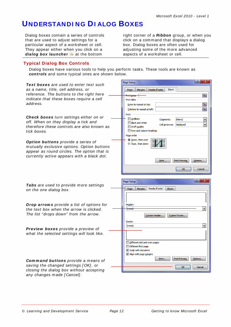
UNDERSTANDING DIALOG BOXES

Dialog boxes contain a series of controls that are used to adjust settings for a particular aspect of a worksheet or cell. They appear either when you click on a dialog box launcher at the bottom

right corner of a Ribbon group, or when you click on a command that displays a dialog box. Dialog boxes are often used for adjusting some of the more advanced aspects of a worksheet or cell.

Typical Dialog Box Controls Dialog boxes have various tools to help you perform tasks. These tools are known as controls and some typical ones are shown below.

Text boxes are used to enter text such as a name, title, cell address, or reference. The buttons to the right here indicate that these boxes require a cell address.

Check boxes turn settings either on or off. When on they display a tick and therefore these controls are also known as tick boxes.

Option buttons provide a series of mutually exclusive options. Option buttons appear as round circles. The option that is currently active appears with a black dot.

Tabs are used to provide more settings on the one dialog box.

Drop arrows provide a list of options for the text box when the arrow is clicked. The list “drops down” from the arrow.

Preview boxes provide a preview of what the selected settings will look like.

Command buttons provide a means of saving the changed settings [OK], or closing the dialog box without accepting any changes made [Cancel].



LAUNCHING DIALOG BOXES

For Your Reference… To launch a dialog box:

1. Click on a dialog box launcher, relevant command button or menu option

Handy to Know… • In some situations the dialog box

launcher actually displays a task pane. For example, if you click on the dialog box launcher in the Clipboard group on the Home tab, the Office Clipboard task pane appears.

1

2

Dialog boxes can be launched either as the result of clicking on a dialog box launcher or a command button, or by selecting a command from a menu. In a menu, the presence of three dots (an

ellipse) ... after a menu option indicates that the menu option, when selected, will display a dialog box. Dialog boxes are generally used for advanced features or detailed settings.

Try This Yourself:


1 Point to the dialog box launcher in the Font group on the Home tab to display a tooltip which explains what will happen

2 Click on the dialog box launcher to display the Format Cells dialog box

This dialog box has a selection of controls to make formatting cells easier...

3 Click on the Border tab

This displays additional controls that you can use to adjust the borders around the active cell or range of cells...

4 Click on [Cancel] to close the dialog box without doing anything

Some commands on the Ribbon automatically launch a dialog box…

5 Click on the Page Layout tab, then click on Print Titles in the Page Setup group to display the Page Setup dialog box

6 Click on [Cancel]



UNDERSTANDING THE QUICK ACCESS TOOLBAR

The Quick Access Toolbar, also known as the QAT, is a small toolbar that appears at the top left-hand corner of the Excel window. It is designed to provide access to the command tools you use frequently,

such as Save, and includes by default the Undo and Redo buttons. You can add more tools to the Quick Access Toolbar to make finding favourite commands easier.

The Quick Access Toolbar The Quick Access Toolbar is positioned at the top left corner of the Microsoft Excel 2010 screen. In its default state, it includes the Save tool, the Undo tool and the Redo tool.

Customising the Quick Access Toolbar Appearing immediately to the right of the Quick Access Toolbar, the Customise Quick Access Toolbar tool displays a list of commonly used commands that you can add to the toolbar. You can select the items that you want to add. The ticks that appear to the left of the menu options show you that an option is already displayed.



ADDING COMMANDS TO THE QAT

Try This Yourself:


1 Point to the first button on the Quick Access Toolbar to see the name of the tool and its shortcut

In this case, it is Save...

2 Right-click on Format Painter which appears in the Clipboard group on the Home tab to display a shortcut menu

3 Select Add to Quick Access Toolbar to add the Format Painter tool to the QAT

4 Click on the Customise Quick Access Toolbar tool

to display the menu

5 Click on Open to add the Open command to the Quick Access Toolbar

It is just as easy to remove tools you don’t want from the QAT...

6 Right click on the Format Painter tool and click on Remove from Quick Access Toolbar

7 Repeat step 6 and remove the Open tool from the QAT

For Your Reference… To customise the Quick Access Toolbar:

1. Right-click on the command you want to add and select Add to Quick Access Toolbar

Or 1. Click on the Customise Quick Access

Toolbar tool and click on a command

Handy to Know… • You can move the QAT under the

ribbon by clicking on the Customise Quick Access Toolbar tool and selecting Show Below the Ribbon. This puts the tools that you use most frequently closer to your document making it quicker to access them.

1

2

The Quick Access Toolbar is a handy location to place commands from the Ribbon that you use most frequently. Adding commands from the Ribbon

involves locating the command, right-clicking it and choosing the Add to Quick Access Toolbar option from the short cut menu that appears.

3

5

7



UNDERSTANDING THE STATUS BAR

The Status Bar is the bar across the bottom of the Excel window. It is a very useful aid that tells you the current status of Excel, performs quick calculations on the selected range in the worksheet, and

allows you to zoom in and out of the worksheet. It also includes tools that can change the worksheet view. You can customise the status bar to change the information shown.

1 Status Indicator

The Status Indicator indicates the current status of Excel and the worksheet. The most common indicator you’ll see here is Ready indicating that Excel is ready and waiting for you to do something.

2 Average This tells you the average value in the cells currently selected in the worksheet – providing the cells contain numeric data. Selected cells are the ones that have the active cell indicator around them and are commonly referred to as a range of cells. Obviously for a calculation to be performed there will need to be numbers in the active range of cells.

3 Count This tells you how many non-empty cells are in the cells currently selected in the worksheet.

4 Sum This tells you the sum total of the cells currently selected in the worksheet – providing the cells contain numeric data.

5 View Tools The Worksheet View tools allow you to change the view of the worksheet. You can select from Normal, Page Layout, and Page Break Preview.

6 Zoom Level This button displays the current zoom percentage. If you click on the button, the Zoom dialog box will appear so that you can select a specific zoom percentage.

7 Zoom Slider The Zoom Slider indicates the current zoom level, where the centre mark indicates 100%. You can either drag the marker to the left or right, or click on a specific point of the slider to set a zoom percentage. You can also click on the buttons at either end of the slider to zoom in or zoom out .

8 Resize Icon The Resize icon is visible in the Excel window if the screen is not maximised. It allows you to change the size of the window by dragging in or out.

1 2 3 4 5 6 7 8

What appears on the status bar can vary greatly. Don’t be alarmed if the one on your screen doesn’t exactly match the status bar example shown above. For your status bar to match the one above you will need to enter numbers into a range of cells and switch certain status bar indicators on and others off. The one above is shown as a representative example of what can appear on a status bar.



EXITING SAFELY FROM EXCEL

Try This Yourself:


1 Click in cell A1 (the top left cell), type your name and press

Doing this has made a change to your workbook which should be picked up when you attempt to exit…

2 Click on the File tab and click on the Exit quick command at the right of the screen

You will now be prompted to save your workbook if you wish to retain your data. The message you receive will be one of the ones shown – don’t worry about the difference between them for now (you’ll learn more about them later).

We have no reason for keeping a workbook with our name in it so we won’t bother saving…

3 Click on [Don’t Save] to exit from Excel

For Your Reference… To safely exit from Microsoft Excel 2010:

1. Click on the File tab and click on the Exit quick command

2. If you want to keep your changes click on [Save] then specify a workbook name and location, otherwise click on [Don’t Save]

Handy to Know… • Whenever you are in doubt about

whether to save or not you should err on the side of caution and save the workbook. You can delete unwanted workbooks at a later date, but you can seldom retrieve data that has not been saved!

1

2

When you are finished working with Excel you’ll find there are several ways to exit from it. If you have made changes to the worksheet Excel will ask if you wish to save these changes before exiting. You’ll

learn all about saving a little later on. If you don’t wish to retain any changes you’ve made you can decline Excel’s offer to save your work.

You’ll receive a message either like this…

Or like this…



CONCLUDING REMARKS

Congratulations! You have now completed the Getting to know Microsoft Excel booklet. This booklet was designed to get you to the point where you can competently perform a variety of operations as listed in the objectives on page 2.

We have tried to build up your skills and knowledge by having you work through specific tasks. The step by step approach will serve as a reference for you when you need to repeat a task.

Where To From Here… The following is a little advice about what to do next:

• Spend some time playing with what you have learnt. You should reinforce the skills that you have acquired and use some of the application's commands. This will test just how much of the concepts and features have stuck! Don't try a big task just yet if you can avoid it - small is a good way to start.

• Some aspects of the course may now be a little vague. Go over some of the points that you may be unclear about. Use the examples and exercises in these notes and have another go - these step-by-step notes were designed to help you in the classroom and in the work place!

Here are a few techniques and strategies that we've found handy for learning more about technology:

• visit CLD’s e-learning zone on the Intranet

• read computer magazines - there are often useful articles about specific techniques

• if you have the skills and facilities, browse the Internet, specifically the technical pages of the application that you have just learnt

• take an interest in what your work colleagues have done and how they did it - we don't suggest that you plagiarise but you can certainly learn from the techniques of others

• if your software came with a manual (which is rare nowadays) spend a bit of time each day reading a few pages. Then try the techniques out straight away - over a period of time you'll learn a lot this way

• and of course, there are also more courses and booklets for you to work through

• finally, don’t forget to contact CLD’s IT Training Helpdesk on 01243-752100

Microsoft Excel 2010 – Level 1 Learning Guides... · Microsoft Excel 2010 ... Microsoft Office....

Documents

Transcript of Microsoft Excel 2010 – Level 1 Learning Guides... · Microsoft Excel 2010 ... Microsoft Office....