Microgravity investigations of instability and mixing flux...

1. Introduction

Fundamental results of microgravity investigations serve as a

powerful tool, which could help to solve modern problems of

terrestrial engineering and technology. Flows in porous media

could be much better understood in microgravity studies elimi-

nating the masking effects of gravity.

In frontal displacement of a more dense and viscous fluid by

a less dense and viscous one the Rayleigh-Taylor or Saffman-

Taylor instability of the interface could bring to formation and

growth of "fingers" of gas penetrating the bulk fluid. The

growth of fingers and their further coalescence could not be des-

cribed by the linear analysis. Growth of fingers causes irregula-

rity of the mixing zone. The tangential velocity difference on

the interface separating fluids of different density and viscosity

could bring to a Kelvin-Helmholtz instability resulting in "dif-

fusion of fingers" partial regularization of the displacement

mixing zone. Thus combination of the two effects would govern

the flow in the displacement process1-7.

The problem is relevant to a hydrocarbon recovery, which is

performed by the flow of gas under a pressure differential

displacing the high viscosity fluid. There are inherent instabili-

ty and scalability problems associated with viscous fingering

that play a key role in the procedure. Entrapment of high visco-

sity fluid by the low viscosity fluid flow lowers down the qua-

lity of a hydrocarbon recovery leaving the most of viscous fluid

entrapped thus decreasing the production rate. The gravity

effects could play essential role because the problem is scale

dependent.

The developed models and obtained results are applicable to

description of liquid non-aqueous phase contaminants under-

ground migration, their entrapment in the zones of inhomogeni-

ty, and forecasting the results of remediatory activities in the

vicinities of waste storages and contaminated sites.

Another important application of the obtained results is the

problem of delivering water to the roots of plants in irrigated

Smirnov N.N.(1), Nikitin V.F.(1), Ivashnyov O.E.(1), Maximenko A.(2) , Thiercelin M.(2)

Vedernikov A. (3), Scheid B. (3), Legros J.C. (3)

Microgravity Investigations of Instability and

Mixing Flux in Frontal Displacement of Fluids

The goal of the present study is to investigate analytically,numerically and experimentally the instability of the displace-ment of viscous fluid by a less viscous one in a two-dimensionalchannel, and to determine characteristic size of entrapmentzones. Experiments on miscible displacement of fluids in Hele-Shaw cells were conducted under microgravity conditions.Extensive direct numerical simulations allowed to investigatethe sensitivity of the displacement process to variation of valuesof the main governing parameters. Validation of the code wasperformed by comparing the results of model problems simula-tions with experiments and with the existing solutions publishedin literature. Taking into account non-linear effects in fluidsdisplacement allowed to explain new experimental results onthe pear-shape of fingers and periodical separation of their tipelements from the main body of displacing fluid. Those separa-ted blobs of less viscous fluid move much faster than the meanflow of the displaced viscous fluid. The results of numericalsimulations processed based on the dimensions analysis allowto introduce criteria characterizing the quality of displacement.The functional dependence of the dimensionless criteria on thevalues of governing parameters needs further investigations.

Smirnov N.N. et al: Microgravity Investigations of Instability and Mixing Flux in Frontal Displacement of Fluids

© Z-Tec Publishing, Bremen Microgravity sci. technol. XV/2 (2004) 35

Mail address: (1) Faculty of Mech. and Math., Moscow M.V.Lomonosov State University,

Moscow 119992, Russia(2) Schlumberger Moscow Research, Hydrokorpus, Leninskie Gory 1-19,

Moscow 119992, Russia(3) Microgravity Research Centre, Free University of Brussels, CP 165/62

Brussels 1050, Belgium

Paper submitted: 05.10.2003

Submission of final revised version: 19.04.2004

Paper accepted: 21.04.2004

zones. The entrapment of water in porous soils governs the sup-

ply of plants' root zones.

2. Experiments on Fluid Displacement in a Hele-Shaw Cell

For experimental modeling of flows in porous media Hele-

Shaw cells are used, wherein a small distance between the pla-

tes creates enormous drag forces thus simulating the effect of

porous media resisting the fluid flow. Fluid flow in a horizon-

tally placed Hele-Shaw cell is usually gravity irrelevant for very

thin cells, wherein viscous forces are predominant as related to

buoyancy ones. The dimensionless criterion characterizing the

ratio of viscous and gravity forces in a Hele-Shaw cell has the

following form:

which is, actually, the ratio of Frude and Reynolds numbers.

Here μ is fluid viscosity, u - fluid velocity, ρ =⏐ρ1 - ρ2⏐ - the

density difference at the phase interface (if one fluid is air then

ρ is equal to the density of the other fluid, g is gravity accelera-

tion, h - cell thickness. For flows in porous media Vg >> 1. The

dimensionless criterion inversely depends on cell thickness in

the second power and on gravity acceleration in the first power.

Investigating the flow patterns in a Hele-Shaw cell it is neces-

sary sometimes to increase the cell thickness, while determining

the correlation between the cell thickness and the width of

viscous fingers. To keep the value of Vg criterion at the same

level for a set of experiments one needs on increasing cell thik-

kness to reduce essentially gravity acceleration. To have the

comparable experimental data one needs to maintain other

parameters: viscosity, flow rate - constant. Thus increasing 4

times the cell thickness one needs to perform 16 times gravity

reduction, which could be done in parabolic flights.

The microgravity experiments were performed in the frame-

work of the 25th ESA parabolic flight campaign of the Airbus

A300 Zero-G (Fig.1) and are shortly described in13, 14.

The Hele-Shaw cell presented in Fig.2 was built of two plates

of 10 mm thick Lexan glass that were 150x200 mm² (a). They

were separated by a spacer (b) that is 25 mm wide and closes

three sides of the cell. Two spacers of different width were used

in order to vary the cell width δ, namely 1.2 and 3.7 mm.

Rubber sheets were placed on both sides of the spacer for leak-

proofness. All together was fixed with screws (c) spaced every

25 mm along the edges. The injection side was screwed on a slot

valve (d) and was proof thanks to an o-ring pressed around the

injection slot. This latter was 100 mm large and 4 mm high. The

inlet was then planar on the contrary of the outlet that was a 5

mm diameter hole (e) in the bottom of lexan plate. In order to

prevent the influence of the outlet geometry on the linear stre-

amlines, cavities (f) were drilled on all the width in the lexan

plate, perpendicularly, just before the outlet, as drawn on the

bottom plate in Fig. 2.

The injection phase performed under microgravity conditions

is shown in Fig. 5. The displacing fluid, namely dyed water, is

flowing into the circuit numbered "1". The flow rate is control-

led by the rotating pump and ranged from 0.6 ml/s to 18.5 ml/s.

The liquid was injected uniformly into the cell by the slot valve.

It displaced the steady pre-filling fluid of water-glycerine solu-

tion. The punctual outlet was connected to a trash tank.

The characteristic dimensions of the fluid filled domain L x Hx δ were: length L = 200mm, width H = 100mm. Thickness δvaried in different experiments. Besides mean flow velocity U= Q / (Hδ) and viscosity ratio M =μ2 /μ1 were also varied in

experiments. Table 1 gives the description of 10 experiments,

which results are illustrated in Fig. 3 in the form of two succes-

sive pictures of the displacement front for times t1 and t2 for

each experiment. The succession of images in Fig. 3 corre-

sponds to their numbers in the table 1.

Microgravity sci. technol. XV/2 (2004)36


u FrVg ,

gh² Re

μ= =ρ

Fig. 2. Experimental cell: (a) Lexan plate - (b) surrounding spacer in Lexan- (c) screw - (d) slot valve - (e) hole - (f) cavity - (g) pump. The circuit "1" isfor injection and the "2" is for cleaning/fillingFig. 1. The Novespace Airbus A-300 Zero-G performing a parabolic flight.


Microgravity sci. technol. XV/2 (2004) 37

The results of experiments show, that all the parameters under

investigation produce an effect on the displacement process. For

high viscosity ratio fingers have pear-shaped form with the

heads separating and continuing independent motion as blobs of

less viscous fluid moving through a more viscous one. Such

separated blobs are clearly seen in Fig. 3.3. This is in a good

coincidence with our numerical results, which showed that the

head of a pear-shaped finger separates and moves independent-

ly advancing in a more viscous fluid under the influence of the

imposed pressure gradient.

The instability in displacement of a viscous fluid by a less

viscous one brings to the formation of a mixing zone.

As it is seen from Fig. 3 the thickness of the fingers λ essen-

tially depends on viscosity ratio M =μ2 /μ1. Fig. 4 illustrates the

mean dimensionless thickness of fingers λ /δ as a function of

M1/4 obtained by averaging the experimental data for different

flow velocity U and gap width δ. The results illustrated in Fig.

4 confirm that for the present experimental conditions (high

Peclet numbers) all the dependencies are practically linear and

have similar inclination. Thus the dependence could be appro-

ximated by the following function:

λ /δ = 0.35 (M1/4-1).

Fig. 3. The succession of flow images for different cases of displacement ofa viscous fluid by a less viscous one. The experimental conditions are provi-ded in the table 1.

Fig. 4. The mean dimensionless thickness of fingers as a function of viscosi-ty ratio in the power 1/4 for different experiments: Curve 1 - U= 1 cm/s, δ =1,2 mm; Curve 2 - U= 1 cm/s, δ = 3,7 mm; Curve 3-U= 2.75 cm/s, δ = 1,2mm; Curve 4 - U= 2.75 cm/s, δ = 3,7 mm; Curve 5 - U= 5 cm/s, δ = 1,2mm.

Fig.5. Saturation maps for viscous fluids displacement: viscosity ratio M=1,dimensionless time τ = t - U / L = 0.219.

#

1

2

3

4

5

6

7

8

9

10

M

84

84

84

9

3

84

84

9

9

3

U. cm/s

5

2.75

1

5

5

2.75

1

1

1

2.75

δ, mm

1.2

1.2

1.2

1.2

1.2

3.7

3.7

3.7

1.2

1.2

t1, s

0.4

0.8

2

0.4

0.4

0.8

2

2

2

0.8

t2, s

1.6

3.2

8

1.6

1.6

3.2

8

8

8

3.2

Table 1

3. Mathematical Model

In the dimensionless form, it is reduced to the following system

of equations, boundary and initial conditions:

μ (s) = M -s ; (4)

x = 0, x = A · Pe: y = ± Pe/2: ψ = y; (5)

x = 0: s = 1; x =A · Pe: ∂s / ∂x = 0; (6)

y = ±Pe/2: ∂s / ∂y = 0; (7)

t = 0: s = 0 (8)

The equation (1) is related to distribution of the stream function

ψ; it is derived from the Darcy law, the incompressibility and

the absence of gravity force conditions. The expressions (2) are

related to definition of the stream function. The equation (3) sta-

tes for the intruding fluid saturation dynamics. The expression

(4) determines dimensionless fluid viscosity depending on satu-

ration (more saturation, less viscosity; the type of dependence

generalizes harmonic averaging). The boundary conditions (5)

state for solidity of lateral walls at y = ±Pe/2 and regularity of

intruding fluid flow at the inlet (x = 0) and outlet (x = A ·Pe)

boundaries. The boundary conditions (6), (7) state for the inflow

of the intruding fluid only, free outflow of the mixture, von

Neumann's conditions for the saturation affected by diffusion on

the lateral walls. The initial condition (8) says that the domain

is not filled with the intruding fluid at the first instance. The co-

ordinate system origin is placed in the middle of the inlet sec-

tion.

The equation (1), expression (2) and boundary conditions (5)

were derived from the continuity equation, Darcy law and the

non-permeability of lateral walls, correspondingly:

y = ±Pe/2: v = 0 ; (11)

The dimensionless parameters in the relationships (1)-(7) are

determined as follows:

where L, H are the length and the width of the domain, μ1, μ2are viscosity of intruding and displaced fluids, respectively, Q is

the amount of intruding fluid per time unit, U is the average

velocity of insertion.

The following scaling factors are used to derive dimensional

values from dimensionless ones:

Here, values with a bar denote the dimensional parameters rela-



Fig. 6. Saturation maps for viscous fluids displacement: viscosity ratioM=84, dimensionless time τ = t - U / L: a - 0.121; b- 0.248; c- 0.389

0,u vx y

∂ ∂+ =∂ ∂

1 1, ,

p pu vx y

μ μ− −∂ ∂= − = −∂ ∂

2

1

; ;L Q UHA M PeH D D

μμ

= = = =

· , · , · ,

· , · ,²

Du U u v U v x xU

D Dy y t t DU U

ψ ψ

= = =

= = =

( ) ( ) ² ²,

² ²

s us vs s st x y x y

∂ ∂ ∂ ∂ ∂+ + = +∂ ∂ ∂ ∂ ∂

, ,u vy xψ ψ∂ ∂= = −

∂ ∂

( ) ( ) 0,∂ ∂ ∂ ∂+ =∂ ∂ ∂ ∂

s sx x y y

ψ ψμ μ (1)

(2)

(9)

(10)

(12)

(13)

(3)



Fig. 7. Different flow patterns in displacement of viscous fluid by a less viscous one from homogeneous media.

ting to dimensionless ones without the bar over them.

Dimensionless viscosity μ is proportional to the dimensional

one μ⎯ and is scaled upon the viscosity of the fluid being displa-

ced and permeability K of the porous skeleton:

4. Numerical Modeling

Numerical simulations were performed in a 2-D domain having

original size 200 mm x 100 mm, which corresponds to the expe-

rimental cell described above. Numerical modeling was perfor-

med for the case of a homogeneously permeable medium,

which corresponds to a Hele-Shaw cell with flat parallel walls,

and for the cases of inhomogeneous permeability as well, which

corresponds to the case of obstacle placing in the gap between

the two walls in the Hele-Shaw cell. To simulate inhomogene-

ous permeability 5x5 mm obstacles were used15, which perme-

ability was assumed two orders of magnitude lower than the one

in the rest of the computational domain. The placing of obsta-

cles was 10 or 11 in a row depending on parity. Computational

domain grid was 201 x 101 with 5x5 cells obstacles and 5 cells

average distance between obstacles edges. Aspect ratio A=2,

Peclet number Pe=10000. We used Eulerian approach to solve

the problem stated above; the rectangular grid with uniform

space steps was involved. Using CFL (Courant - Friedrichs -

Levi) criterion we determined the next time step value9. Using

2D TVD (2-dimensional total variation diminishing) techniques

of the second order10 we transferred the hyperbolic part of the

concentration equation (3) to the next time layer. Using 2D

Buleev technique (implicit iterative method for elliptic equa-

tions using incomplete factorisation11 we transfer the parabolic

part of the concentration equation (3) to the next time layer.

5. Displacement from Homogenous Media

Results of numerical simulations described and analyzed below

are relevant to the instability in displacement of miscible fluids,

when there is no distinct fluid-fluid interface and fluids could

penetrate into each other due to diffusion. Investigating instabi-

lity in miscible displacement differs greatly from that in immi-

scible fluids. The presence of a small parameter incorporating

surface tension for immiscible fluids allows to determine theo-

retically the characteristic shape and width of viscous fingers16,

17, while in miscible fluids theoretical analysis allows to fore-

cast the shape of the tips, but does not allow to determine the

width of fingers, which remains a free parameter18, 19. Results of

extensive numerical simulations of viscous fingering in immi-

scible displacement20 have capillary number being one of model

parameters, while the present paper deals with miscible fluids

displacement characterized by a different set of model parame-

ters incorporating Peclet number.

Numerical modeling of displacement for fluids of equal

viscosity was carried out to validate the scheme. The results

shown in Fig. 5 testify, that the displacement is stable for the

viscosity ratio M=1. Numerical scheme under consideration

does not introduce any instability.

As it is known, the increase of viscosity ratio for the displa-

ced and displacing fluids promotes instability in frontal displa-

cement from a homogeneous medium. Fig. 6 illustrates the satu-

ration maps for successive times for the case of high viscosity

ratio M=84. To provide a better illustration the characteristic

time in displaying results is different from that used in (13),

which has a more explicit physical meaning: τ = t ·U / L = t⎯ /Pe.

The results show, that the interface instability arising in

viscous fluids displacement (for M >1) brings to formation of

fingers of less viscous fluid penetrating the more viscous one.

Those fingers grow in time. Some of fingers have the tendency

to acquire a peer-shape with the neck getting thinner, and then

separate from the displacing fluid. Those separated blobs of less

viscous fluid move independently through the more viscous one

under the influence of imposed pressure gradient as if floating

up in the gravity field. In time mixing of low viscosity fluid with

the surrounding one takes place due to diffusion, and the blobs

slow down to the velocity of the flow. The traces of the separa-

ted blobs, which diffused before, serve as a preferable pathway

for new fingers to develop.

Numerical experiments were carried out to investigate the

influence of dimensionless governing parameters - Peclet num-

ber and viscosity ratio - on the structure of displacement flow

and the mixing flux caused by phase interface instability and

formation of fingers. The results are shown in the Fig.7, which

illustrates characteristic flow patterns obtained for different



Fig. 8. Saturation of the intrusive fluid for an aspect ratio A=12; viscosityratio and Peclet number: M = 20, Pe = 1024.

2

·Kμ μμ

=

values of governing parameters. The aspect ratio was assumed

to be equal to A=1.

Fig. 8 illustrates saturation of the intrusive fluid for a higher

aspect ratio A=12; M = 20; Pe = 1024. It is seen that the small

separated blobs of displacing fluid gradually dissolve in the

displaced one. Large portions of displaced fluid are being ent-

rapped by the displacing one and move at a much lower veloci-

ty than the mean velocity of displacement.

6. Width-Averaged Intrusive Fluid Saturation

The definition of width-averaged saturation of the intrusive

fluid was given in our previous report. Using the present nota-

tions, it can be written as follows:

The average saturation < s > defined in (14) characterises 1D

distribution of the intrusive fluid along the porous domain;

many significant values can be expressed in terms of it: the

displacement front location and dispersion, the mixing zone

length, the amount of displaced fluid trapped in the porous

domain behind the displacement front, and so on. This parame-

ter can be easily derived from the solution of 2D problem but

our goal is to create a 1D model describing its behaviour

without using multidimensional computations. The only way to

do this is to set some dynamical model calculating behaviour of

a parameter c(t, x) depending on some unknown coefficients βnand then choose the set of βn influencing c(t, x) which minimi-

ses a generalised difference between c and <s>. For example,

such a functional can be of the least-squares cost function type:

The expression (15) determines the averaged square of diffe-

rence between derived and modelled width-averaged intrusive

fluid saturation. Because of discrete representation of spatially

distributed parameters in the numerical model, the integrals in

(14)-(15) can be changed by sums, and the final expression for

the functional to be minimised will be as follows:

Here, tk (k = 1,..., m) are specified characteristic times, sij is cal-

culated saturation at x = xi , y = yi, ci is modelled saturation at x= xi; the least two relating to the same time moments tk.

The mixing zone length Z can be estimated as follows:

where ε is a small threshold number (e.g. one per cent). It turns

that the mixing zone length depends on the value of ε, and we

will reference to it as Zε.

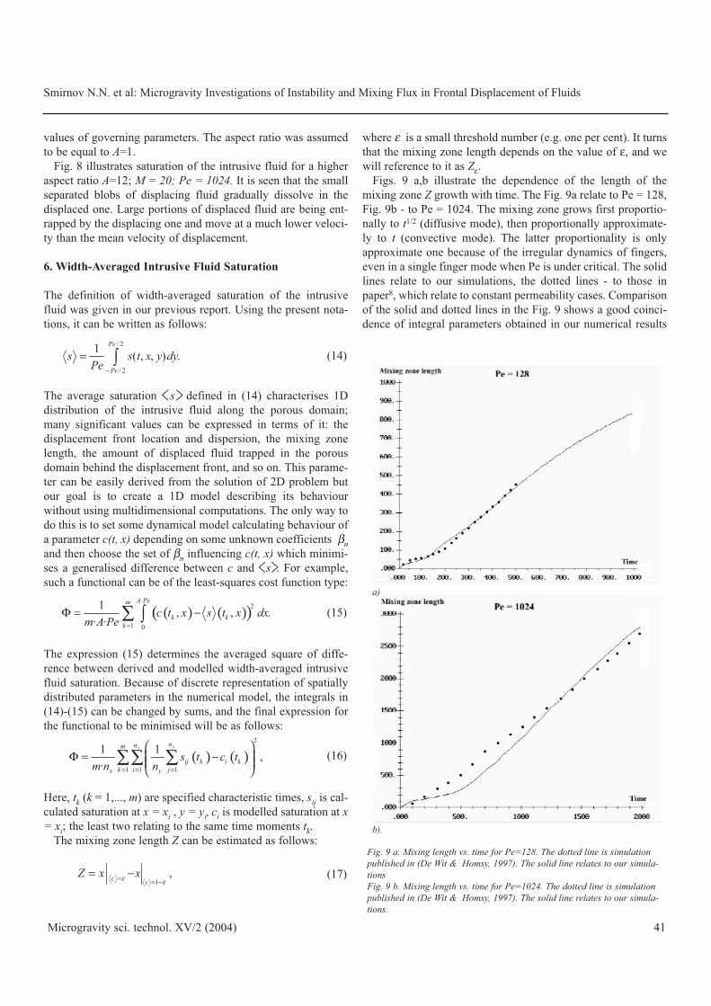
Figs. 9 a,b illustrate the dependence of the length of the

mixing zone Z growth with time. The Fig. 9a relate to Pe = 128,

Fig. 9b - to Pe = 1024. The mixing zone grows first proportio-

nally to t1/2 (diffusive mode), then proportionally approximate-

ly to t (convective mode). The latter proportionality is only

approximate one because of the irregular dynamics of fingers,

even in a single finger mode when Pe is under critical. The solid

lines relate to our simulations, the dotted lines - to those in

paper8, which relate to constant permeability cases. Comparison

of the solid and dotted lines in the Fig. 9 shows a good coinci-

dence of integral parameters obtained in our numerical results



/ 2

/ 2

1( , , ) .

Pe

Pe

s s t x y dyPe −

= ∫

( ) ( )( )·

2

1 0

1, , .

· ·

A Pem

k kk

c t x s t x dxm A Pe =

Φ = −∑ ∫

( ) ( )2

1 1 1

1 1,

·

yx nnm

ij k i kk i jx y

s t c tm n n= = =

⎛ ⎞Φ = −⎜ ⎟⎜ ⎟⎝ ⎠

∑∑ ∑

1,c c

Z x xε ε= = −= −

Fig. 9 a. Mixing length vs. time for Pe=128. The dotted line is simulationpublished in (De Wit & Homsy, 1997). The solid line relates to our simula-tionsFig. 9 b. Mixing length vs. time for Pe=1024. The dotted line is simulationpublished in (De Wit & Homsy, 1997). The solid line relates to our simula-tions.

a)

b).

(14)

(15)

(16)

(17)

with that obtained by other methods. It is seen from Fig. 9 a,b

that a good agreement on the mixing zone length is achieved.

The difference between the curves obtained in paper8 and in our

simulations can be explained by different factor used to break

up the unstable equilibrium and obtain the fingers: slightly

disturbed initial conditions in paper8 and randomly disturbed

permeability in the present paper. Moreover, we processed our

simulations in the case of small Peclet number to t = 1000 and

it is seen from Fig. 9a that the convective behaviour of the

mixing zone (its length being proportional to time), which esta-

blished by t = 500 gradually changes back for the dispersive one

(Z proportional to the square root of time). This comparison ser-

ves a good verification for the codes.

Comparison of our results with that obtained in paper8 shows

that for high Peclet numbers similar behaviour of fingers could

be noticed: their number decreases in time and only 3 or 4 fin-

gers remain active. On the other hand, contrary to paper8 in our

simulations the results are not symmetrical: fingers laying close

to upper and lower boundaries of the domain have better chan-

ce to survive. In the long run the finger attached to one of the

sides of the domain can finally supersede other fingers.

Reynolds Approach to 1D Averaged Model

Introducing the width averaging operator similar to one applied

to s in the expression (14),

we derive the behavior of averaged parameters directly from the

original multidimensional system of equations. Let us denote a

perturbation of a parameter ϕ with ϕ´. The perturbation can be

defined as difference between actual and averaged values: ϕ´ =

ϕ - <ϕ> . Then, by definition we have the following properties:

<<ϕ>> = <ϕ>, <ϕ´>=0, <ϕ1ϕ2> =<ϕ1><ϕ2>+ <ϕ1´ϕ2´>.similar to the properties of Reynolds averaging which are being

applied to turbulent flows investigation.

Applying the averaging operator to the continuity equation

(9) and taking boundary conditions (11) into account, one

obtains that the average of horizontal velocity is constant

along the length of the domain, and it is equal to unit in our

method of scaling:

≡ 1.

Applying the averaging operator to the saturation equation (3)

and taking boundary conditions (6), (7) and (11) into account,

we get the following equation describing behavior of < s >:

The equation (18) was obtained taking into account non-perme-

ability of lateral walls (eliminating convective flux in the lateral

direction) and von Neumann's conditions for saturation on late-

ral walls (eliminating the second (diffusion) term). Note that the

equation (18) is a typical equation for a scalar average value

behavior in a turbulent flow: left side terms stand for convec-

tion, the first right hand side term is the turbulent mixing (or

dispersion) as the opposite to the derivative of the turbulent

flux, the second stands for laminar diffusion. The relating theo-

ries for turbulent flow then could be taken into account.

The diffusive approach to model the turbulent flux < u’ s’>is based on the Prandtl hypothesis. If we apply it, we get:

where DT is the turbulent diffusion factor which must be mode-

led itself. Either additional equations or simple algebraic

expressions are used to model it in different theories of turbu-

lent mixing. In order to develop such a phenomenology,

unknown coefficients regulating some empirical dependence of

DT must be introduced as well. These coefficients could be cho-

sen so as to minimize the difference between the solution deri-

ved from multidimensional computations, which model the

behavior of the actual parameters (analog of DNS for turbulent

flow investigations), and 1D computations modeling the mean

values of parameters (analog of a phenomenological theory

application).

Using the equality ≡ 1 for mean velocity and the Prandtl

hypothesis (19) for turbulent flux of saturation, and choosing an

algebraic expression for turbulent diffusion depending on satu-

ration, we can rearrange the terms in (18) so that it takes the

form:

where c denotes the modelled mean intrusive fluid saturation

(not to mix with the average of 2D modelling solution denoted

with < s >). The turbulent diffusion depends on the mean satu-

ration itself; the dependence is regulated by unknown parame-

ters {βn}.

The boundary and initial conditions for the equation (20) mat-

ching the correspondent conditions (6), (7) and (8) are the fol-

lowing:

x = 0: c = 1, x = A · Pe: (∂c / ∂x) = 0, t=0 : c=0. (21)

In order to get the dependence of mixing coefficient upon c, we

should take into account the following considerations. First, that

the perturbation increases the flux only in the areas of disper-

sion, i.e. where s is neither unit, nor zero. Then it is reasonable

to assume that the simplest types of DT (c) should be:

DT (c) = β1 cβ2 (1 - c)β3. (22)

/ 2

/ 2

1Pe

Pe

dyPe

ϕ ϕ−

= ∫

' ' ².

²

s u s u s st x x x

∂ ∂ ∂ ∂+ = − +

∂ ∂ ∂ ∂

(1 ( )) ,Tc c cD ct x x x

∂ ∂ ∂ ∂+ = +∂ ∂ ∂ ∂

' ' ,T

su s D

x∂

= −∂

Smirnov N.N. et al: : Microgravity Investigations of Instability and Mixing Flux in Frontal Displacement of Fluids

42 Microgravity sci. technol. XV/2 (2004)

(18)

(19)

(20)

Second, it could be assumed that the mixing flux is maximal in

the zones wherein both phases are present in equal portions, i.e.

c ≈ 1/2. The last assumption leads to the condition

β2 = β3.

Another approach allowing to model the turbulent flux is follo-

wing (let us refer it to as the flux approach).

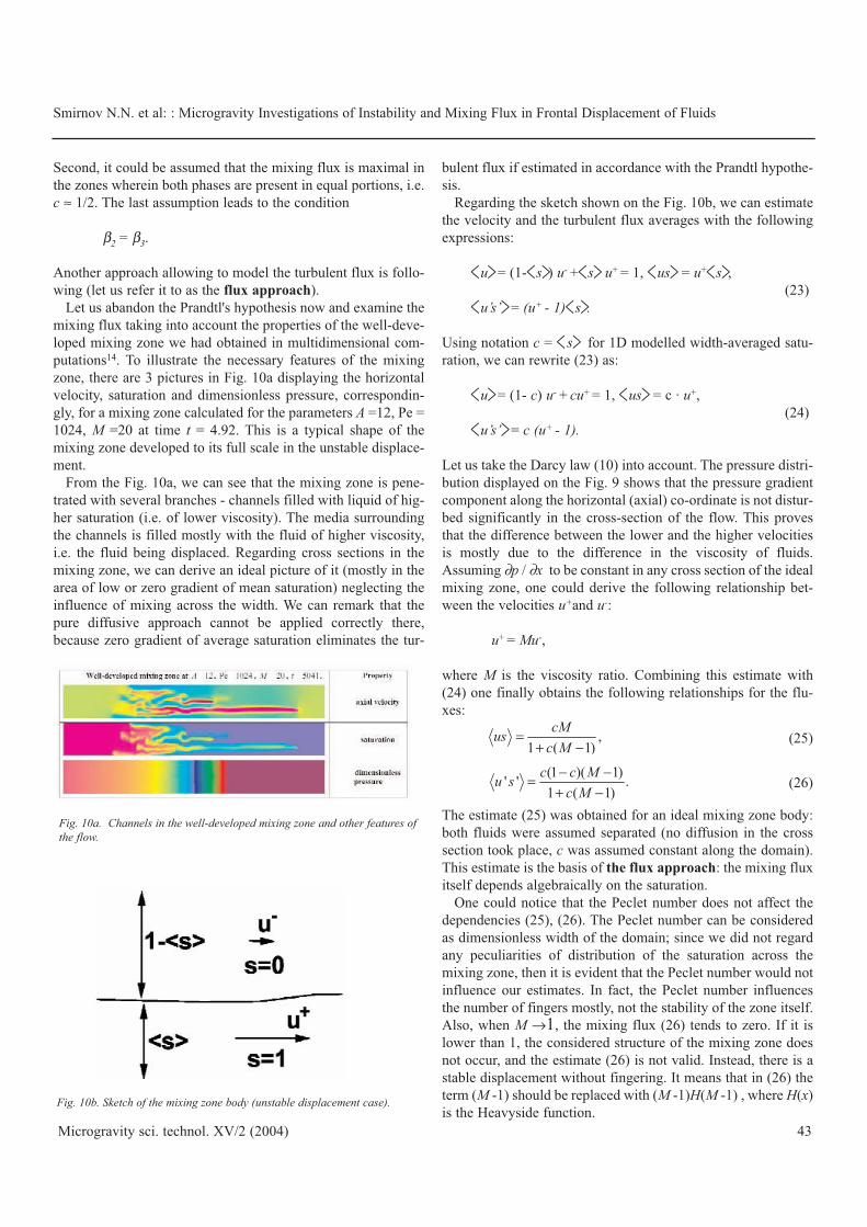
Let us abandon the Prandtl's hypothesis now and examine the

mixing flux taking into account the properties of the well-deve-

loped mixing zone we had obtained in multidimensional com-

putations14. To illustrate the necessary features of the mixing

zone, there are 3 pictures in Fig. 10a displaying the horizontal

velocity, saturation and dimensionless pressure, correspondin-

gly, for a mixing zone calculated for the parameters A =12, Pe =

1024, M =20 at time t = 4.92. This is a typical shape of the

mixing zone developed to its full scale in the unstable displace-

ment.

From the Fig. 10a, we can see that the mixing zone is pene-

trated with several branches - channels filled with liquid of hig-

her saturation (i.e. of lower viscosity). The media surrounding

the channels is filled mostly with the fluid of higher viscosity,

i.e. the fluid being displaced. Regarding cross sections in the

mixing zone, we can derive an ideal picture of it (mostly in the

area of low or zero gradient of mean saturation) neglecting the

influence of mixing across the width. We can remark that the

pure diffusive approach cannot be applied correctly there,

because zero gradient of average saturation eliminates the tur-

bulent flux if estimated in accordance with the Prandtl hypothe-

sis.

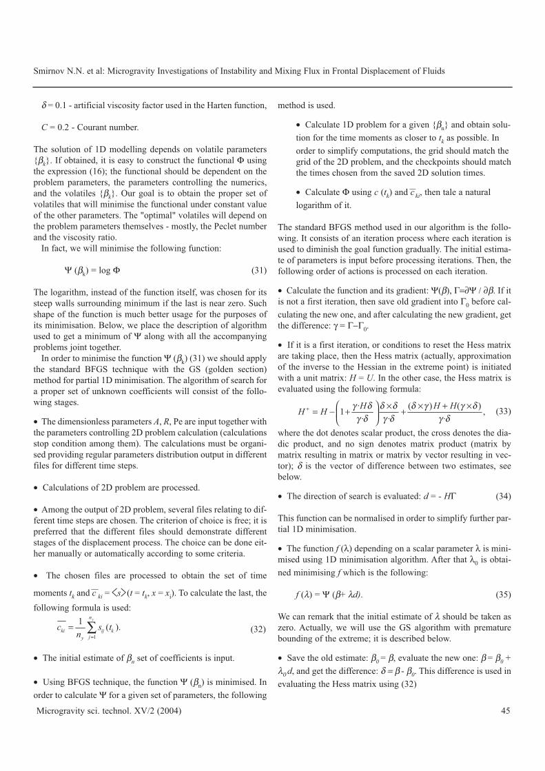
Regarding the sketch shown on the Fig. 10b, we can estimate

the velocity and the turbulent flux averages with the following

expressions:

= (1-<s>) u- +<s> u+ = 1, <us> = u+<s>,

(23)

<u’s’>= (u+ - 1)<s>.

Using notation c = < s> for 1D modelled width-averaged satu-

ration, we can rewrite (23) as:

= (1- c) u- + cu+ = 1, <us> = c · u+,

(24)

<u’s’>= c (u+ - 1).

Let us take the Darcy law (10) into account. The pressure distri-

bution displayed on the Fig. 9 shows that the pressure gradient

component along the horizontal (axial) co-ordinate is not distur-

bed significantly in the cross-section of the flow. This proves

that the difference between the lower and the higher velocities

is mostly due to the difference in the viscosity of fluids.

Assuming ∂p / ∂x to be constant in any cross section of the ideal

mixing zone, one could derive the following relationship bet-

ween the velocities u+and u-:

u+ = Mu-,

where M is the viscosity ratio. Combining this estimate with

(24) one finally obtains the following relationships for the flu-

xes:

The estimate (25) was obtained for an ideal mixing zone body:

both fluids were assumed separated (no diffusion in the cross

section took place, c was assumed constant along the domain).

This estimate is the basis of the flux approach: the mixing flux

itself depends algebraically on the saturation.

One could notice that the Peclet number does not affect the

dependencies (25), (26). The Peclet number can be considered

as dimensionless width of the domain; since we did not regard

any peculiarities of distribution of the saturation across the

mixing zone, then it is evident that the Peclet number would not

influence our estimates. In fact, the Peclet number influences

the number of fingers mostly, not the stability of the zone itself.

Also, when M →1, the mixing flux (26) tends to zero. If it is

lower than 1, the considered structure of the mixing zone does

not occur, and the estimate (26) is not valid. Instead, there is a

stable displacement without fingering. It means that in (26) the

term (M -1) should be replaced with (M -1)H(M -1) , where H(x)

is the Heavyside function.

,1 ( 1)

cMusc M

=+ −

(1 )( 1)' ' .

1 ( 1)

c c Mu sc M

− −=+ −

Fig. 10b. Sketch of the mixing zone body (unstable displacement case).

Fig. 10a. Channels in the well-developed mixing zone and other features ofthe flow.

Smirnov N.N. et al: : Microgravity Investigations of Instability and Mixing Flux in Frontal Displacement of Fluids

43Microgravity sci. technol. XV/2 (2004)

(25)

(26)

Combined approach. Let us examine the drawbacks and

advantages of the flux and the diffusive approaches. First, one

can see that the diffusive approach (if single-equation model is

considered, of course) can work well only if the gradient of

width-averaged saturation is not zero. But the main body of the

developed mixing zone has the gradient near zero, and even at

zero gradient, the mixing flux may not be zero at all (this was

shown in our considerations of the flux approach). This draw-

back could be remedied replacing the diffusive approach by the

flux approach, but the last has its own disadvantages.

Let us examine the expression (25), which stands for the total

flux. Since this expression is an algebraic one, then the effecti-

ve velocity of small disturbances propagation (the "sound velo-

city", or the flux jacobian eigenvalue) should be the partial deri-

vative of the expression (25) by c:

At c = 1, M =1, this velocity equals to unit (this correlates with

the velocity of displacement equal to unit), but at low c the

value of a tends to M. The value of M is not bounded from

above, so in case of high viscosity ratio, the velocity of distur-

bances propagation at the tip of the mixing zone is unrealisti-

cally high. This result was obtained as a consequence of the fact

that we did not regard the lateral diffusion and some other fac-

tors bounding the intrusive channel width in the mixing zone

from below. So, the flux approach without improvements is also

not an ideal one.

In order to diminish drawbacks of the diffusive and the flux

approaches, it is worth to combine them involving scalar weight

coefficients. In general, it means that we should model the

mixing flux using two empirical dependencies:

where FT should be referenced to as mixing convective flux and

DT- as mixing diffusion factor. Both of them depend explicitly

on the averaged saturation. In order to model this dependence,

rational expression like (26) can be taken for the convective

flux, and a polynom - for the diffusion factor. With the expres-

sion (28), the original equation (18) modeling averaged satura-

tion behavior is transformed to:

We suggest to use the following expressions for FT and DT as

a first order approximation:

The expressions (30) are rather simple, they were obtained

using considerations described above. The diffusive coefficient

is expressed via a simplified polynomial form as compared with

(22). The solution of (29)-(30) with the boundary conditions

(21) is unique for a set of unknown coefficients {α, β} = { βk},

if the coefficients {α, β} are set non-negative; however it is not

a strict necessity condition.

Computational Techniques for Mixing Flux Modelling

To process 1D calculations, the following algorithm was app-

lied.

1. Input the grid {xi} and time checkpoints {tk} : 0 < t1< ...<

tm ; input A, M, Pe.

2. Input {βk}. Separated from the item 1 because of multiple

return possibility.

3. Construct the initial state: t0 = 0, {ci0}.

4. Transition from n-th to (n+1)-th time layer: {cin}→ {ci

n+1},

tn+1=tn + Δt:

(a) Obtain time step Δt according to modified Courant -

Friedrichs - Levy criterion:

Δt= C min (Δxi / Qδ (ai)),

where Qδ (x) is the Harten function depending on the para-

meter δ regulating artificial viscosity in TVD techniques 1

order step, a is the "sound velocity" - derivative of satura-

tion flux upon saturation. C < 1 is a constant (Courant

number).

(b) Process explicitly the convective step, using TVD

techniques of the 2nd order.

(c) Process implicitly the diffusive step using Thomas

algorithm to solve 3-diagonal linear equations. The transi

tion coefficient is taken from previous iteration.

(d) Recalculate the transition coefficient and process anot

her one iteration (steps b and c) until the number of itera

tions is three.

5. Examine the next time checkpoint: if tn < tk ≤ tn+1, then

interpolate linearly the solutions {cin} and {ci

n+1} onto the

time layer tk. Save the result into {cik}.

6. If the last time checkpoint is passed, then stop. Else, go to

the next time layer (item 4).

The process is governed, along with the problem parameters, by

the grid distribution, time checkpoints positions, the set of { βk},

and the following control parameters, which are maintained

constant:

.(1 ( 1))²

us Mac c M

∂= =

∂ + −

' ' ( ) ( ) ,T Tcu s F c D cx

∂= −∂



( ( ))(1 ( )) ,T

Tc F cc cD c

t x x x∂ +∂ ∂ ∂+ = +

∂ ∂ ∂ ∂

(1 )( 1)( ) , ( ) ²(1 )²,

1 ( 1)T T

c c MF c D c ßc cc M

α − −= = −+ −

(27)

(28)

(29)

(30)

δ = 0.1 - artificial viscosity factor used in the Harten function,

C = 0.2 - Courant number.

The solution of 1D modelling depends on volatile parameters

{βk}. If obtained, it is easy to construct the functional Φ using

the expression (16); the functional should be dependent on the

problem parameters, the parameters controlling the numerics,

and the volatiles {βk}. Our goal is to obtain the proper set of

volatiles that will minimise the functional under constant value

of the other parameters. The "optimal" volatiles will depend on

the problem parameters themselves - mostly, the Peclet number

and the viscosity ratio.

In fact, we will minimise the following function:

Ψ (βk) = log Φ (31)

The logarithm, instead of the function itself, was chosen for its

steep walls surrounding minimum if the last is near zero. Such

shape of the function is much better usage for the purposes of

its minimisation. Below, we place the description of algorithm

used to get a minimum of Ψ along with all the accompanying

problems joint together.

In order to minimise the function Ψ (βk) (31) we should apply

the standard BFGS technique with the GS (golden section)

method for partial 1D minimisation. The algorithm of search for

a proper set of unknown coefficients will consist of the follo-

wing stages.

• The dimensionless parameters A, R, Pe are input together with

the parameters controlling 2D problem calculation (calculations

stop condition among them). The calculations must be organi-

sed providing regular parameters distribution output in different

files for different time steps.

• Calculations of 2D problem are processed.

• Among the output of 2D problem, several files relating to dif-

ferent time steps are chosen. The criterion of choice is free; it is

preferred that the different files should demonstrate different

stages of the displacement process. The choice can be done eit-

her manually or automatically according to some criteria.

• The chosen files are processed to obtain the set of time

moments tk and c⎯ki = <s>(t = tk, x = xi). To calculate the last, the

following formula is used:

• The initial estimate of βn set of coefficients is input.

• Using BFGS technique, the function Ψ (βn) is minimised. In

order to calculate Ψ for a given set of parameters, the following

method is used.

• Calculate 1D problem for a given {βn} and obtain solu-

tion for the time moments as closer to tk as possible. In

order to simplify computations, the grid should match the

grid of the 2D problem, and the checkpoints should match

the times chosen from the saved 2D solution times.

• Calculate Φ using c (tk) and c⎯ki, then tale a natural

logarithm of it.

The standard BFGS method used in our algorithm is the follo-

wing. It consists of an iteration process where each iteration is

used to diminish the goal function gradually. The initial estima-

te of parameters is input before processing iterations. Then, the

following order of actions is processed on each iteration.

• Calculate the function and its gradient: Ψ(β), Γ=∂Ψ / ∂β. If it

is not a first iteration, then save old gradient into Γ0 before cal-

culating the new one, and after calculating the new gradient, get

the difference: γ = Γ−Γ0.

• If it is a first iteration, or conditions to reset the Hess matrix

are taking place, then the Hess matrix (actually, approximation

of the inverse to the Hessian in the extreme point) is initiated

with a unit matrix: H = U. In the other case, the Hess matrix is

evaluated using the following formula:

where the dot denotes scalar product, the cross denotes the dia-

dic product, and no sign denotes matrix product (matrix by

matrix resulting in matrix or matrix by vector resulting in vec-

tor); δ is the vector of difference between two estimates, see

below.

• The direction of search is evaluated: d = - HΓ (34)

This function can be normalised in order to simplify further par-

tial 1D minimisation.

• The function f (λ) depending on a scalar parameter λ is mini-

mised using 1D minimisation algorithm. After that λ0 is obtai-

ned minimising f which is the following:

f (λ) = Ψ (β+ λd). (35)

We can remark that the initial estimate of λ should be taken as

zero. Actually, we will use the GS algorithm with premature

bounding of the extreme; it is described below.

• Save the old estimate: β0 = β, evaluate the new one: β = β0 +λ0 d, and get the difference: δ = β - β0. This difference is used in

evaluating the Hess matrix using (32)



1

1( ).

yn

ki ij kjy

c s tn =

= ∑

· ( ) ( )1 ,

· · ·

H H HH H γ δ δ δ δ γ γ δγ δ γ δ γ δ

+ ⎛ ⎞ × × + ×= − + +⎜ ⎟⎝ ⎠

(32)

(33)

• Check the criterion of iterations break (one can use δ and the

tolerances set input beforehand). Also, one can check the follo-

wing: if λ0 is negative, then it is time to reset the Hess matrix

into unit on the next iteration. If the iteration process is not to be

broken, go to next iteration.

We can remark that each of the iterations of the BFGS method

requires N +1 evaluations of the functional Ψ where N is the

number of parameters βn (not including the number of iterations

on 1D minimisation stage). Those evaluations require solution

of 1D problem from t = 0 to t = tm, therefore it is the most time

consuming part of the process.

The algorithm of 1D minimisation using golden section tech-

niques for bounded extreme and bounding technique before

applying GS, being applied to a function f (λ) with initial esti-

mate equal to zero and initial value of function f 0= f (0) regar-

ded as known, can be described as follows.

• Bounding stage.

• Input initial Δ (argument increment), λ- =-Δ, λ+ = Δ,

• Evaluate f - = f (λ−), f + = f (λ+) .

• If f - > f0 and f + > f0 then the extreme is bounded within

the segment [λ-, λ+]; no other processing on the bounding

stage is needed. Else, determine the direction of search

(positive if f + < f0 ; negative if f - < f0 ; if both are lower, then

the direction points to the lowest of them).

• In case of the negative direction, exchange λ+ ↔ λ-, f+ ↔ f - and alter the sign of Δ.

• Process the cycle of bounding. On each iteration:

• Store successively: λ− = λ0, λ0 = λ+; f− = f 0, f 0 = f+.

Evaluate λ+ = λ0 + Δ, f+ = f(λ+).

• If f+ > f 0, then the extreme is bounded between λ− and

λ+. Otherwise, increase Δ← 2Δ and repeat the cycle. Note:

the cycle will finish only if the function has a real minimum

not in the infinity. To stop infinite cycling one can break the

cycle either after a definite number of iterations or after excee-

ding a definite absolute value of λ+.

• After processing the bounding algorithm, the bounds λ− and

λ+ are not necessarily ordered first lower second higher. The fol-

lowing GS algorithm does not require this order.

• Golden section minimisation algorithm. On input, we have

λ− and λ+ bounding the extreme point. Then, the following cycle

is processed while ⏐ λ+−λ−⏐ exceeds some given tolerance.

• Evaluate a = g1λ− + g2λ+, b = g1λ+ + g2λ− , where g1= 0.618,

g2 = 0.382 (golden section proportions). Then, evaluate fa = f (a),

fb = f (b).

• If fa > fb , then set λ− = a. Otherwise, set λ+ = b.

• Repeat the cycle, if the difference exceeds tolerance.

Otherwise, return either a or b depending on the result of pre-

vious comparison. One should not return an average because it

is not guaranteed with sure that function of it is less than the

evaluated one.

The 1D-minimisation stage requires 2 + nb evaluations of func-

tion on the bounding stage and 2ns evaluations on the GS stage;

nb, ns are numbers of iterations at each stage, correspondingly.

To reduce the job, a proper value of initial increment Δ must be

set: too low brings to high number of iterations on the bounding

stage, too high increases iterations number on the GS stage. The

value of tolerance affects the GS stage number of iterations

only: it is proportional to logarithm of the tolerance.

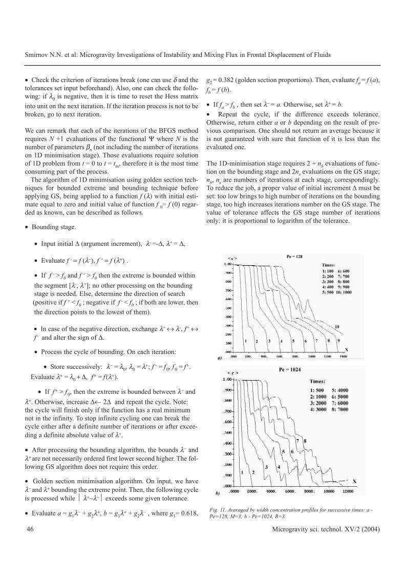
Fig. 11. Averaged by width concentration profiles for successive times: a -Pe=128, M=3; b - Pe=1024, R=3.

Results of Multidimensional Modeling Processing Aimed at

Developing Mixing Flux Coefficients

The technique described above was applied to search for proper

coefficients of the turbulent flux and the turbulent diffusion

coefficient (30). At first, we obtained the following results for

α ≡ 0 (diffusive approach case).

The Figs. 11a, b illustrate the behaviour of concentration ave-

raged across the width of the domain. In spite of disturbances

caused by arbitrary fingering, it develops regularly enough to

have a chance to be described by the developed techniques. One

can see that the behaviour of the averaged concentration is

much more regular and therefore predictable in case of sub-cri-

tical Peclet number (Fig. 11a). The Fig. 11a relates to Pe =128,M = 20, Fig. 11b - to Pe = 1024, M = 20. The behaviour of ave-

raged concentration for supercritical Peclet number is much

more irregular: non-monotonous disturbances rise up from

t=2000 (curve 3) and develop further.

The table beside contains the diffusion coefficient obtained

for different M and Pe, and the fit quality (contrary to

Ψ function, which decreases on increasing the fit quality, the

present parameter grows higher the better the fit is).

Each entry in the Table 2 relating to one pair of Pe, M consists

of two numbers: the coefficient itself placed above and the cor-

responding fit quality below.

Together with the main tendency of rising β with Pe and M,

the table 2 shows some anomaly results. The first anomaly is

situated in the right lower corner, it shows a very good qualities

of fit (orders of magnitude higher as being compared to the

other entries) but almost zero value of the coefficient. It means

that under those conditions, the regular displacement took place

almost without motion in lateral directions. In this case, the

width-averaged saturation coincides with the saturation itself.

The second is higher coefficient at Pe = 256, M = 3 than at Pe =

512, M = 3, contradictory to the main tendency. However, the

quality of fit is good in both cases. Maybe, it could be explained

by some unresolved tendency of the coefficient behaviour near

the critical curve separating zones of regular and irregular

displacement.

Table 2. Diffusive approach case. Coefficient ß and the fit quality

1024

512

256

128

20.09

4787

5.50

2058

5.46

985.4

4.93

489.5

5.20

7.39

2461

5.76

1472

5.62

727.4

4.86

165.9

5.24

4.48

1920

6.33

728.0

5.61

446.1

5.28

86.11

5.89

3.00

1067

6.65

320.2

5.92

420.1

6.95

0.22

12.94

Diffusion coefficient and fit quality. Diffusive approach case

Viscosity ratio MPe

Fig. 12. Evolution of the fingering index with time for different viscosityratios.

Fig. 13. Regular (a) and randomized (b) obstacles placing in the computa-tional domain.



8. Integral Characteristcs of Displacement Process

The following integral dimensionless parameters are to be tra-

ced with time to provide the characteristics for the displacement

procedure12 .

Displacement QualityThe amount of fluid 2 remaining in the domain characterises

the quality of displacement. It is calculated as:

where the integral scopes the whole domain. The initial amount

is equal to the dimensionless volume in the domain.

Fingering indexThis is a special parameter proportional to ratio of the dimen-

sionless interface surface within the domain to the volume of

the domain. The increase of interface instability leads to the

increase of this index. The magnitude of it will be referenced to

as F.

In order to compute the fingering index, a rectangular grid is

required in the domain. Then, if the parameter c = αij is deter-

mined in the nodes of the grid, the fingering index is calculated

as follows:

where ni, nj are numbers of grid nodes in horizontal and vertical

directions. The description of the fingering index above looks

like slightly modified definition of the total variation of α by

Yee, Warming and Harten (1985)10. Plots of the fingering index

changing with time for different values of are shown on the fig.

12. To obtain results on mixing induced purely by instability

diffusive mixing was assumed to be zero for the present run

(infinite Peclet number)12. The curves obtained have similar

properties: first the curves rise up to maximal values then slight-

ly decrease. It can be seen from the Fig. 12 that the increase of

the viscosity ratio M increases the fingering index.

9. Displacement from Inhomogenous Media

To simulate inhomogeneous permeability 5x5 mm obstacles

were used, which permeability was assumed two orders of mag-

nitude lower. The obstacles placing is shown in Fig. 13. Both

regular and randomized sets of obstacles within a Hele-Shaw

cell were investigated. In all the runs of numerical simulations

the same pattern of randomized obstacles was used.

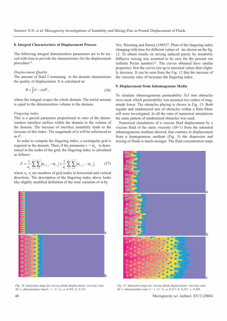
Numerical simulations of a viscous fluid displacement by a

viscous fluid of the same viscosity (M=1) from the saturated

inhomogeneous medium showed, that contrary to displacement

from a homogeneous medium (Fig. 5) the dispersion and

mixing of fluids is much stronger. The fluid concentration maps

Fig. 14. Saturation maps for viscous fluids displacement: viscosity ratioM=1, dimensionless timeτ = t - U / L: a- 0.053; b- 0.181.

Fig. 15. Saturation maps for viscous fluids displacement: viscosity ratioM=1, dimensionless time τ = t - U / L: a- 0.117; b- 0.167; c- 0.504.



(1 ) ,B c dV= −∫

11

1, , , 1 ,

1 1 1 1

1 1,

y yx xn nn n

i j i j i j i jj i i jy x

Fn n

α α α α−−

+ += = = =

= − + −∑∑ ∑ ∑

(36)

(37)

for displacement from inhomogeneous samples with regular

obstacles placing are shown in Fig. 14. As it is seen from the

Fig. 14 the flow branching effect due to inhomogenity of per-

meability brings to a much stronger dispersion of fluids and to

a sharp increase of the mixing zone.

Irregularity in obstacles placing increases the dispersion even

more for the present numerical experiment (Fig. 15).

Based on the results of numerical simulations described

above one could come to the conclusion that regular and irregu-

lar inhomogenity of permeability both promote flow instability

and formation of a mixing zone due to fluids dispersion. This

conclusion is valid for fluids of low viscosity ratio (practically

equal viscosity).

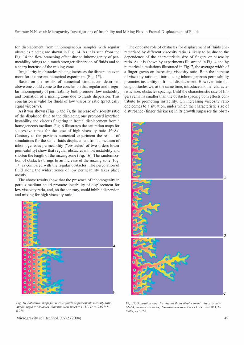
As it was shown (Figs. 6 and 7), the increase of viscosity ratio

of the displaced fluid to the displacing one promoted interface

instability and viscous fingering in frontal displacement from a

homogeneous medium. Fig. 6 illustrates the saturation maps for

successive times for the case of high viscosity ratio M=84.

Contrary to the previous numerical experiment the results of

simulations for the same fluids displacement from a medium of

inhomogeneous permeability ("obstacles" of two orders lower

permeability) show that regular obstacles inhibit instability and

shorten the length of the mixing zone (Fig. 16). The randomiza-

tion of obstacles brings to an increase of the mixing zone (Fig.

17) as compared with the regular obstacles. The percolation of

fluid along the widest zones of low permeability takes place

mostly.

The above results show that the presence of inhomogenity in

porous medium could promote instability of displacement for

low viscosity ratio, and, on the contrary, could inhibit dispersion

and mixing for high viscosity ratio.

The opposite role of obstacles for displacement of fluids cha-

racterised by different viscosity ratio is likely to be due to the

dependence of the characteristic size of fingers on viscosity

ratio. As it is shown by experiments illustrated in Fig. 4 and by

numerical simulations illustrated in Fig. 7, the average width of

a finger grows on increasing viscosity ratio. Both the increase

of viscosity ratio and introducing inhomogeneous permeability

promotes instability in frontal displacement. However, introdu-

cing obstacles we, at the same time, introduce another characte-

ristic size: obstacles spacing. Until the characteristic size of fin-

gers remains smaller than the obstacle spacing both effects con-

tribute to promoting instability. On increasing viscosity ratio

one comes to a situation, under which the characteristic size of

disturbance (finger thickness) in its growth surpasses the obsta-



Fig. 17. Saturation maps for viscous fluids displacement: viscosity ratioM=84, random obstacles, dimensionless time τ = t - U / L: a- 0.053; b-0.089; c- 0.166.

Fig. 16. Saturation maps for viscous fluids displacement: viscosity ratioM=84, regular obstacles, dimensionless timeτ = t - U / L: a- 0.097; b-0.218.

cle spacing. Then due to geometrical constraints displacement

from each gap between neighbouring obstacles should be stable,

because the disturbances, which could grow, surpass the gap

width. However, randomisation of obstacles, brings to forma-

tion of gaps of different width. That creates preferable pathways

for fluids displacement thus promoting instability.

Experimental investigations of the role of inhomogenity was

performed on a similar hardware, but the Hele-Shaw cell itself

contained additional obstacles (Fig. 18). The modified Hele-

Shaw cell with obstacles provides much better conditions for

modelling dispersion in a porous medium than the classical

Hele-Shaw cell. The classical cell without obstacles simulates

drag forces in pore flow, while the cell with obstacles enables to

simulate pore branching as well that is crucial for determining

the mixing flux.

The colour added to the displacing fluid enables to trace the

mixing zone evolution thus providing the data for determining

the mixing coefficient.

The characteristics sizes of the cell: length L = 200 mm, width

B = 100 mm, thickness h = 3.7mm, the size of obstacles 5mm x5mm x 3.7mm. The displacing fluid is delivered from the right

hand side. The sink for the displaced fluid is in the left hand

side of the cell. The fluids are water and water-glycerin solu-

tions that makes it possible to vary the viscosity ratio in a wide

range.

Fig. 18 a, b illustrates the experiment on displacement of a

highly viscous fluid by a less viscous one from a modified Hele-

Shaw cell with obstacles. The flow rate corresponds to a mean

displacement velocity U = 5cm/s. Both figures correspond to

time 0.60 s after the beginning of displacement process. The

viscosity ratio was equal to M = 3 in Fig. 18a, and it was M =84 in Fig. 18b. It is seen that for the present experiment the size

of the mixing zone is larger for the case of lower viscosity ratio.

Investigations of peculiarities of instability in fluids displace-

ment from inhomogeneous porous media should be continued.

The effect of placing obstacles on stabilization of displacement

for high viscosity ratios was also observed in experiments des-

cribed in the paper15, but now the undertaken theoretical inve-

stigations allowed to suggest the explanation for this effect.

10. Conclusions

• Displacement of viscous fluid saturating permeable media

by a less viscous one was investigated experimentally and

simulated numerically for miscible fluids.

• Comparison of experimental results with that of numerical

modeling demonstrated a good coincidence and testified the

adequacy of the developed mathematical model.

• Experimental and numerical investigations showed that

some fingers had the tendency to acquire a peer-shape with

the neck getting thinner, and then separate from the

displacing fluid.

• Experimental and numerical investigations showed that the

thickness of "viscous fingers" increases with the increase of

viscosity ratio.

• The effect of Hele-Shaw cell thickness on viscous fingering

in displacement of miscible fluids was investigated

experimentally. Processing of experimental results allowed

to develop for high Peclet numbers a universal dependency

of mean dimensionless thickness of fingers on viscosity

ratio.

• First experiments in a modified Hele-Shaw cell with

obstacles were conducted and analyzed.

• In displacement of a viscous fluid by a less viscous one

originating fingers can both split and agglomerate. It was

shown that for the regarded values of parameters the

tendency to agglomerate was predominant and the number

of fingers was decreasing until it reached some stable value.

• A universal model was developed, which allows to

determine the mixing zone and the averaged mixing flux

based on the results of multi-dimensional modeling. The

developed model allows to provide quantitative evaluations

for the displacement quality and mixing induced by the

instability in frontal displacement of fluids from

Fig. 18. Flow images for different cases of displacement of a viscous fluidby a less viscous one from a modified Hele-Shaw cell with obstacles. Thedisplacement velocity U = 5 cm/s, time 0.60 s. The viscosity ratio: a - M= 3,b - M = 84.



homogeneous media.

• Experiments show that in a traditional Hele-Shaw cell the

increase of viscosity ratio and Peclet number increases

instability, while in a cell with obstacles the dependency on

viscosity ratio could be quite the opposite.

• The presence of inhomogenity in porous medium

destabilises regular displacement, while it could stabilise an

irregular one under definite conditions.

• Innhomogenity of a definite regularity could stabilise the

displacement of a highly viscous fluid by a less viscous one.

11. Acknowledgements

The authors wish to acknowledge the generous support of

INTAS (Grant Aral 00-1075) NATO Scientific and environ-

mental affairs division (Grant EST.CLG.979157), SSTC

Program of Belgium. The authors wish to thank Schlumberger

for permission to publish the paper. The authors are grateful to

ESA and Novespace for the valuable help in performing experi-

ments under the reduced gravity conditions in parabolic flights

of the Airbus A300 Zero-G.

12. References

[1] Barenblatt G.I., Entov V.M., Ryzhik V.M. Theory of fluids flows through

natural rocks. Kluwer Academic Publishes - Dordrecht / Boston / London,

1990.

[2] Nield D.A., Bejan A. Convection in porous media. Springer-Verlag - New

York / Berlin / Heidelberg / London, 1992.

[3] Bear J., Bachmat Y. Introduction to modelling of transport phenomena in

porous media. Kluwer Academic Publishes - Dordrecht / Boston /

London, 1990.

[4] Kaviany M. Principles of heat transfer in porous media. Dover

Publications Inc. - New York, 1988.

[5] Smirnov N.N., Dushin V.R., Legros J.C., Istasse E., Bosseret N., Mincke J.C., Goodman S. Multiphase flow in porous media - mathematical

model and micro-gravity experiments. Microgravity Science and

Technology, IX(3), 1996, pp. 222-231.

[6] Smirnov N.N., Legros J.C., Nikitin V.F., Istasse E., Norkin A.V., Shevtsova V.M., Kudryavtseva O.V. Capillary driven filtration in porous media.

Microgravity Science and Technology, Hanser Publ., 1999, XII, pp. 23-

35.

[7] Smirnov N.N., Nikitin V.F., Norkin A.V., Kiselev A.B., Legros J.C., IstasseE. Microgravity investigation of capillary forces in porous media. Space

Forum 2000, 6(1-4), pp. 1-10.

[8] De Wit A., Homsy G.M. Viscous fingering in periodically heterogeneous

porous media. Part II. Numerical simulations. J. Chem. Phys. 1997. Vol.

107(22), 9619.

[9] Anderson D.A., Tannenhill J.C., Pletcher R.H. Computational fluid

mechanics and heat transfer. New York, McGraw-Hill, 1984.

[10] Yee H.C., Warming R.F., Harten A. Implicit total variation diminishing

(TVD) schemes for steady-state calculations. Journal of Computational

Physics, 57, pp. 327-360 (1985).

[11] Ilyin V.P. Incomplete factorisation methods for solving algebraic systems.

Moscow, Nauka publishes, 1995 (in Russian).

[12] Nikitin V.F., Smirnov N.N., Legros J.C. Effect of fingering in porous

media. 52-d IAF Congress. Toulouse, 2001, IAF-01-J.4.10.

[13] Vedernikov A., Scheid B., Istasse E., Legros J.C. Viscous fingering in

miscible liquids under microgravity conditions. Physics of Fluids, 2001,

Vol. 13, N9, p. S12.

[14] Smirnov N.N., Nikitin V.F., Ivashnyov O.E., Legros J.C., Vedernikov A., Scheid B., Istasse E. Instability in viscous fluids displacement from

cracks and porous samples. Proc. 53-d IAF Congress, Houston, 2002,

IAC-02-J.2.02., 11p.

[15] Smirnov N.N., J. C. Legros, V. F. Nikitin, E. Istasse, L. Schramm, F. Wassmuth, and D'Arcy Hart. Filtration in Artificial Porous Media and

Natural Sands under Microgravity Conditions. Microgravity sci. technol.

2003, XIV/2, pp. 3-28.

[16] Meiburg, E. & Homsy, G.M. Nonlinear unstable viscous fingers in Hele-

Show flows. II. Numerical simulation. Phys. Fluids 1988, 31(3).

[17] Tanveer, S. Surprises in viscous fingering. J. Fluid Mech.,2000, vol. 409,

p.273.

[18] Zhuravlev, P. Zap Leningrad Com. Inst. 1956, 133, 54 (in Russian).

[19] Saffman, P.G. & Taylor, G.J. The penetration of a fluid into a porous

medium of Hele-Show cell containing a more viscous fluid. Proc. R. Foc.

Zond. 1958, A 245, 312.

[20] Guan X., Pitchumani R. Viscous fingering in a Hele-Shaw cell with

finite viscosity ratio and interfacial tension. ASME Journal of Fluids

Engineering, 2003. Vol. 125, No. 2, pp. 354-364.



Microgravity investigations of instability and mixing flux...

Documents

Transcript of Microgravity investigations of instability and mixing flux...