Michał P. HellerPerimeter Institute for Theoretical Physics, Canada

National Centre for Nuclear Research, Poland

Relativistic hydrodynamics at large gradients

based on1103.3452, 1302.0697, 1409.5087 & 1503.07514

with R. Janik, M. Spaliński and P. Witaszczyk

Hydrodynamization

M. P. Heller, R. A. Janik and P. Witaszczyk,Phys. Rev. Lett. 108, 201602 (2012), 1103.3452

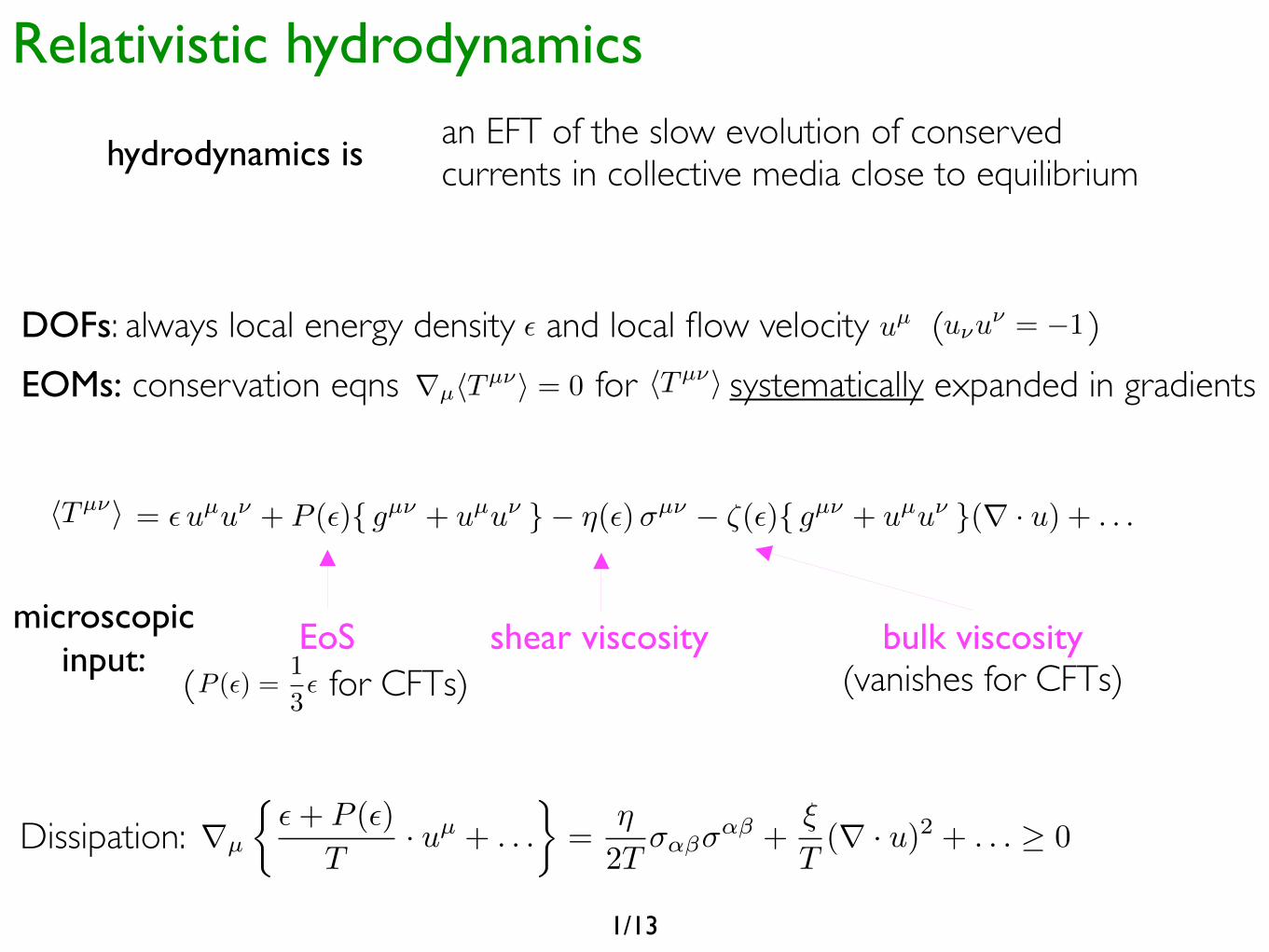
Relativistic hydrodynamicsan EFT of the slow evolution of conserved currents in collective media close to equilibriumhydrodynamics is

DOFs: always local energy density and local flow velocity ( )EOMs: conservation eqns for systematically expanded in gradients

✏ uµ u⌫u⌫ = �1

Tµ⌫ = ✏uµu⌫ + P (✏){ gµ⌫ + uµu⌫ }� ⌘(✏)�µ⌫ � ⇣(✏){ gµ⌫ + uµu⌫ }(r · u) + . . .

shear viscosity bulk viscosity(vanishes for CFTs)

microscopicinput:

EoSP (✏) =

1

3✏( for CFTs)

rµhTµ⌫i = 0 hTµ⌫i

hTµ⌫i

Dissipation: rµ

⇢✏+ P (✏)

T· uµ + . . .

�=

⌘

2T�↵��

↵� +⇠

T(r · u)2 + . . . � 0

1/13

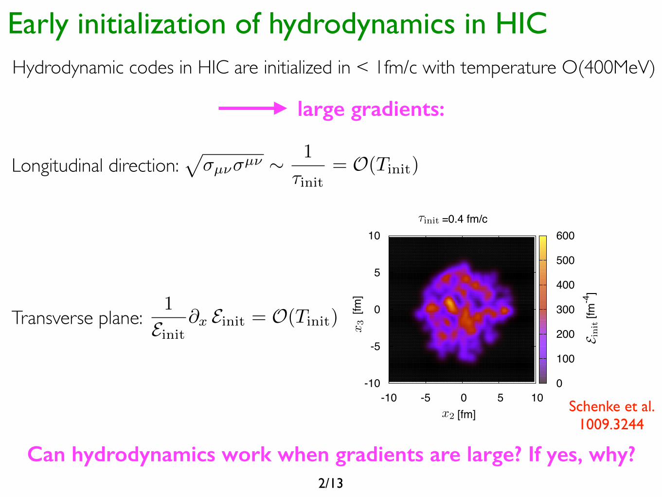
Early initialization of hydrodynamics in HICHydrodynamic codes in HIC are initialized in < 1fm/c with temperature O(400MeV)

Can hydrodynamics work when gradients are large? If yes, why?

2

τ=0.4 fm/c

-10 -5 0 5 10x [fm]

-10

-5

0

5

10

y [fm

]

0

100

200

300

400

500

600

ε [fm

-4]

τ=6.0 fm/c, ideal

-10 -5 0 5 10x [fm]

-10

-5

0

5

10

y [fm

]

0

2

4

6

8

10

12

ε [fm

-4]

τ=6.0 fm/c, η/s=0.16

-10 -5 0 5 10x [fm]

-10

-5

0

5

10

y [fm

]

0

2

4

6

8

10

12

ε [fm

-4]

FIG. 1: (Color online) Energy density distribution in the transverse plane for one event with b = 2.4 fm at the initial time(left), and after τ = 6 fm/c for the ideal case (middle) and with η/s = 0.16 (right).

In this study, we found that setting the local viscosityto zero when finite viscosity causes negative pressure inthe cell as advocated in [25] and reducing the ideal partby 5% works well to stabilize the calculations withoutintroducing spurious effects.While in standard hydrodynamic simulations with av-

eraged initial conditions all odd flow coefficients vanishby definition, fluctuations generate triangular flow v3 asa response to the finite initial triangularity.We follow [15] and define an event plane through the

angle

ψn =1

narctan

⟨pT sin(nφ)⟩⟨pT cos(nφ)⟩

, (9)

where the weight pT is chosen for best accuracy [26].Then, the flow coefficients can be computed using

vn = ⟨cos(n(φ− ψn))⟩ . (10)

The initialization of the energy density is done usinga Glauber Monte-Carlo model (see [27]): Before the col-lision the density distribution of the two nuclei is de-scribed by a Woods-Saxon parametrization, which wesample to determine the positions of individual nucleons.The impact parameter is sampled from the distributionP (b)db = 2bdb/(b2max−b2min), where bmin and bmax dependon the given centrality class. Then we determine the dis-tribution of binary collisions and wounded nucleons. Twonucleons are assumed to collide if their relative transversedistance is less than D =

!

σNN/π, where σNN is the in-elastic nucleon-nucleon cross-section, which at top RHICenergy of

√s = 200AGeV is σNN = 42mb. The energy

density is distributed proportionally to the wounded nu-cleon distribution. For every wounded nucleon we add acontribution to the energy density with Gaussian shape(in x and y) and width σ0 = 0.4 fm. In the rapiditydirection, we assume the energy density to be constanton a central plateau and fall like half-Gaussians at large|ηs| (see [16]). This procedure generates flux-tube likestructures compatible with measured long-range rapiditycorrelations [28–30]. The absolute normalization is deter-mined by demanding that the obtained total multiplicitydistribution reproduces the experimental data.

As equation of state we employ the parametrization“s95p-v1” from [31], obtained from interpolating betweenlattice data and a hadron resonance gas.In Fig. 1 we show the energy density distribution in

the transverse plane for an event with impact parameterb = 2.4 fm at the initial time τ0 = 0.4 fm/c and at timeτ = 6 fm/c for η/s = 0 and η/s = 0.16. This clearlyshows the effect of dissipation.We perform a Cooper-Frye freeze-out using

EdN

d3p=

dN

dypTdpTdφp= gi

"

Σ

f(uµpµ)pµd3Σµ , (11)

where gi is the degeneracy of particle species i, and Σthe freeze-out hyper-surface. In the ideal case the distri-bution function is given by

f(uµpµ) = f0(uµpµ) =

1

(2π)31

exp((uµpµ − µi)/TFO)± 1,

(12)where µi is the chemical potential for particle speciesi and TFO is the freeze-out temperature. In the finiteviscosity case we include viscous corrections to the dis-tribution function, f = f0 + δf , with

δf = f0(1 ± f0)pαpβWαβ

1

2(ϵ+ P)T 2, (13)

where W is the viscous correction introduced in Eq. (5).Note that the choice δf ∼ p2 is not unique [32].The algorithm used to determine the freeze-out surface

Σ has been presented in [16]. It is very efficient in de-termining the freeze-out surface of a system with fluctu-ating initial conditions. To demonstrate this, we presentthe freeze-out surface in the x-τ -plane in the vicinity ofy = 0 fm and ηs = 0 for two different initial distribu-tions compared to that for an averaged initial conditionin Fig. 2. The arrows are projections of the normal vectoron the hyper-surface element onto the x-τ plane.We include resonances up to the φ-meson. We found

that the pseudorapidity dependence of both v2 and v3 isaffected notably by the inclusion of resonance decays, im-proving the agreement of v2(ηp) with data significantly.

large gradients:

Longitudinal direction:

Transverse plane:

Schenke et al. 1009.3244

x2

x

3

E init

⌧init

1

Einit @x Einit = O(Tinit)

p�µ⌫�µ⌫ ⇠ 1

⌧init= O(Tinit)

2/13

x

0

x

1x

1

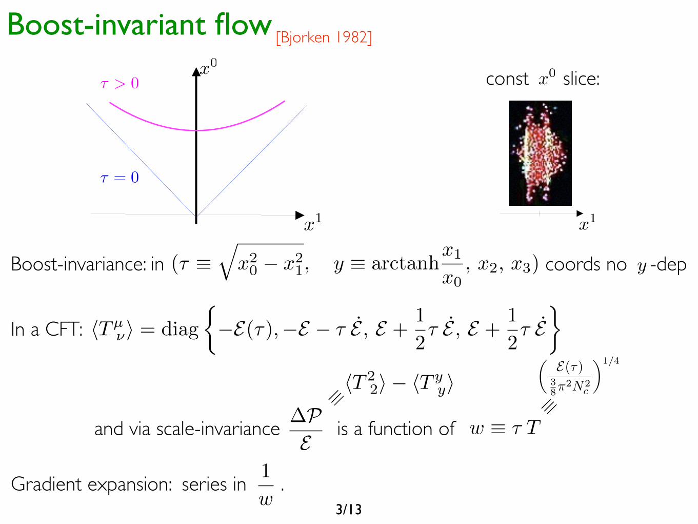
Boost-invariance: in coords no -dep

[Bjorken 1982]

In a CFT:

⌧ = 0

Boost-invariant flow

⌧ > 0

3/13

x

0const slice:

(⌧ ⌘q

x

20 � x

21, y ⌘ arctanh

x1

x0, x2, x3) y

hTµ⌫i = diag

⇢�E(⌧),�E � ⌧ E , E +

1

2⌧ E , E +

1

2⌧ E

�

and via scale-invariance is a function of �PE

hT 22i � hT y

yi⌘w ⌘ ⌧ T

✓E(⌧)

38⇡

2N2c

◆1/4

⌘

Gradient expansion: series in .1

w

Hydrodynamization

4/13

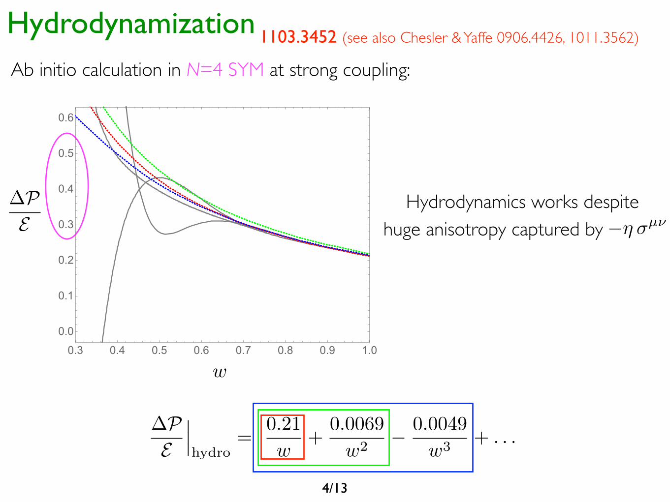
1103.3452 (see also Chesler & Yaffe 0906.4426, 1011.3562)

w

�PE

�PE

���hydro

=0.21

w+

0.0069

w2

� 0.0049

w3

+ . . .

Hydrodynamics works despitehuge anisotropy captured by �⌘ �µ⌫

Ab initio calculation in N=4 SYM at strong coupling:

0.3 0.4 0.5 0.6 0.7 0.8 0.9 1.0

0.0

0.1

0.2

0.3

0.4

0.5

0.6

Why hydrodynamization can occur?

M. P. Heller, R. A. Janik and P. Witaszczyk, Phys. Rev. Lett. 110, 211602 (2013), 1302.0697

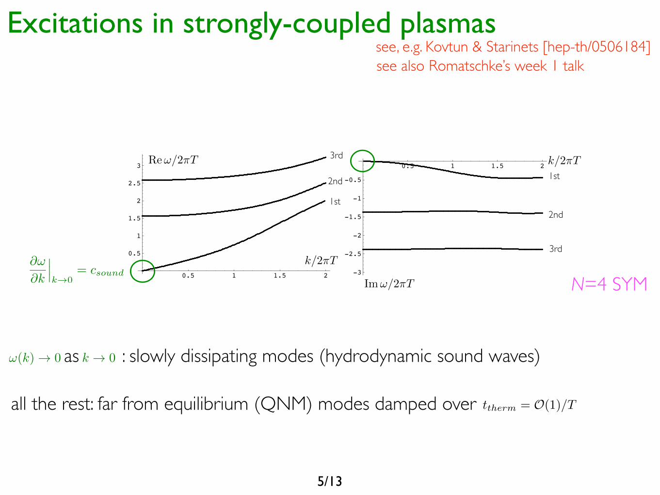
Excitations in strongly-coupled plasmassee, e.g. Kovtun & Starinets [hep-th/0506184]

0.5 1 1.5 2

0.5

1

1.5

2

2.5

3 Re 0.5 1 1.5 2

-3

-2.5

-2

-1.5

-1

-0.5

Im

Figure 6: Real and imaginary parts of three lowest quasinormal frequencies as function of spatialmomentum. The curves for which →0 as →0 correspond to hydrodynamic sound mode in the dualfinite temperature N=4 SYM theory.

behavior of the lowest (hydrodynamic) frequency which is absent for Eα and Z3. For Ez and

Z1, hydrodynamic frequencies are purely imaginary (given by Eqs. (4.16) and (4.32) for small

ω and q), and presumably move off to infinity as q becomes large. For Z2, the hydrodynamic

frequency has both real and imaginary parts (given by Eq. (4.44) for small ω and q), and

eventually (for large q) becomes indistinguishable in the tower of other eigenfrequencies. As an

example, dispersion relations for the three lowest quasinormal frequencies in the sound channel

(including the one of the sound wave) are shown in Fig. 6. The tables below give numerical

values of quasinormal frequencies for = 1. Only non-hydrodynamic frequencies are shown

in the tables. The position of hydrodynamic frequencies at = 1 is = −3.250637i for the

R-charge diffusive mode, = −0.598066i for the shear mode, and = ±0.741420−0.286280i

for the sound mode. The numerical values of the lowest five (non-hydrodynamic) quasinormal

frequencies for electromagnetic perturbations are:

Transverse channel Diffusive channel

n Re Im Re Im

1 ±1.547187 −0.849723 ±1.147831 −0.559204

2 ±2.398903 −1.874343 ±1.910006 −1.758065

3 ±3.323229 −2.894901 ±2.903293 −2.891681

4 ±4.276431 −3.909583 ±3.928555 −3.943386

5 ±5.244062 −4.920336 ±4.946818 −4.965186

and for gravitational perturbations are:

Scalar channel Shear channel Sound channel

n Re Im Re Im Re Im

1 ±1.954331 −1.267327 ±1.759116 −1.291594 ±1.733511 −1.343008

2 ±2.880263 −2.297957 ±2.733081 −2.330405 ±2.705540 −2.357062

3 ±3.836632 −3.314907 ±3.715933 −3.345343 ±3.689392 −3.363863

4 ±4.807392 −4.325871 ±4.703643 −4.353487 ±4.678736 −4.367981

5 ±5.786182 −5.333622 ±5.694472 −5.358205 ±5.671091 −5.370784

– 26 –

Im!/2⇡T

Re!/2⇡T

k/2⇡T

k/2⇡T

1st

2nd

3rd

1st

2nd

3rd

!(k) ! 0 as : slowly dissipating modes (hydrodynamic sound waves)k ! 0

all the rest: far from equilibrium (QNM) modes damped over

@!

@k

���k!0

= csound

ttherm = O(1)/T

5/13

see also Romatschke’s week 1 talk

N=4 SYM

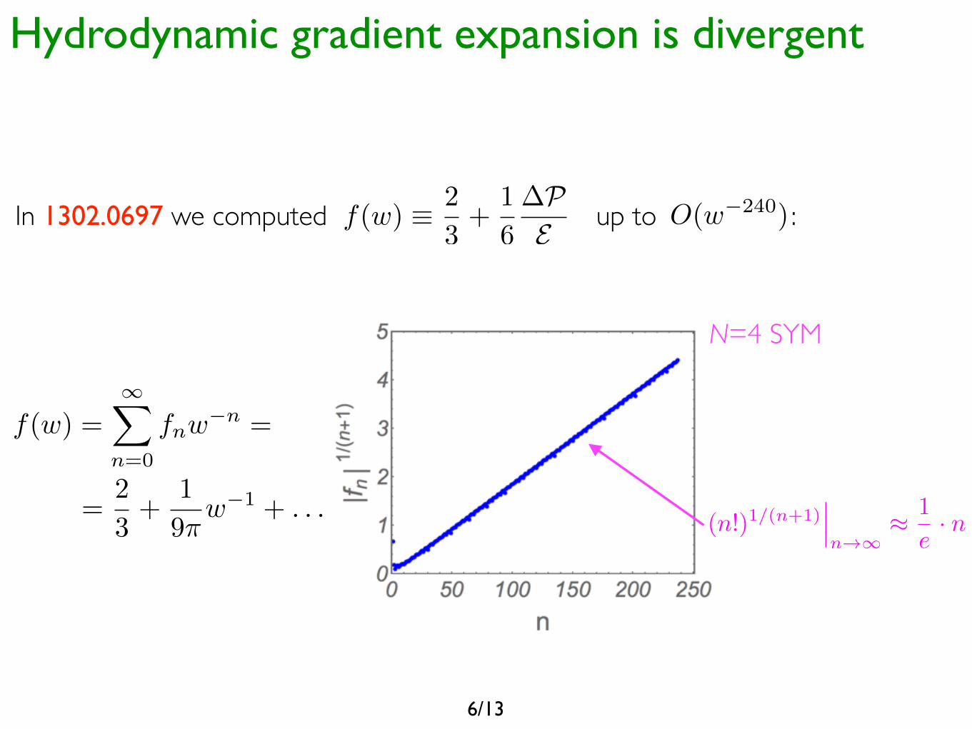
Hydrodynamic gradient expansion is divergent

In 1302.0697 we computed up to :O(w�240)

f(w) =1X

n=0

fnw�n =

=2

3+

1

9⇡w�1 + . . .

(n!)1/(n+1)���n!1

⇡ 1

e· n

6/13

f(w) ⌘ 2

3+

1

6

�PE

N=4 SYM

Hydrodynamics and QNMs

Analytic continuation of revealed the following singularities:fB(⇠) ⇡240X

n=0

1

n!fn ⇠

n

Branch cut singularities start at !3

2i!QNM1

7/13

N=4 SYM

1302.0697

EOMs for viscous hydroand quasinormal modes

M. P. Heller, R. A. Janik, M. Spaliński and P. Witaszczyk,Phys. Rev. Lett. 113, 261601 (2014), 1409.5087

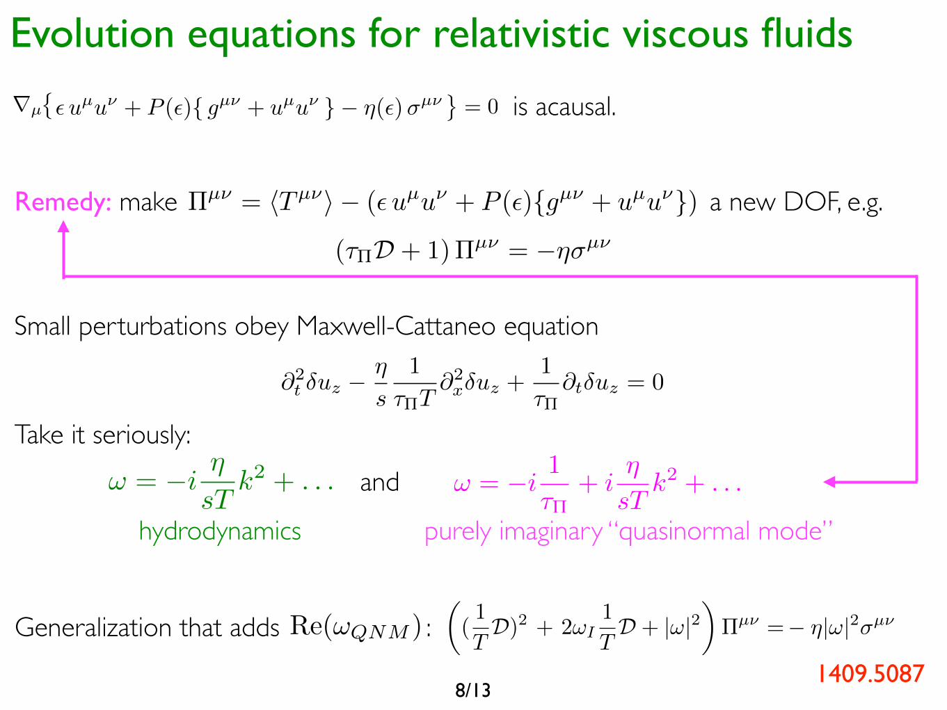
Evolution equations for relativistic viscous fluids

Tµ⌫ = ✏uµu⌫ + P (✏){ gµ⌫ + uµu⌫ }� ⌘(✏)�µ⌫ � ⇣(✏){ gµ⌫ + uµu⌫ }(r · u) + . . .rµ

� = 0

Remedy: make a new DOF, e.g. ⇧µ⌫ = hTµ⌫i � (✏uµu⌫ + P (✏){gµ⌫ + uµu⌫})

Small perturbations obey Maxwell-Cattaneo equation

8/13

(⌧⇧D + 1)⇧µ⌫ = �⌘�µ⌫

@2t

�uz

� ⌘

s

1

⌧⇧T@2x

�uz

+1

⌧⇧@t

�uz

= 0

and! = �i⌘

sTk2 + . . .

hydrodynamics purely imaginary “quasinormal mode”

! = �i1

⌧⇧+ i

⌘

sTk2 + . . .

Take it seriously:

is acausal.

4

situations, where only a single QNM dominates the ap-proach to equilibrium. Setting vanishing initial condi-tions for ⇧µ⌫ reduces the theory to standard MIS, whileincorporating some nontrivial initial conditions allows usto examine the physical e↵ects of the least damped non-hydrodynamic degrees of freedom. This theory could beused as an alternative to MIS hydrodynamics in situa-tions, when an account of early pre-equilibrium dynamicsincluding modes with <(!) 6= 0 is relevant. We performvarious tests of this theory in the following section.

Before that however, we would like to mention a pos-sible alternative which aims to get rid of the nonphysicalMIS mode altogether and use the physical nonequilib-rium degrees of freedom as a means of ensuring hyper-bolicity. Note that since the QNM have a sizable realfrequency, one can never describe them using the MIS de-caying mode. This has already been emphasized in [19].

Heuristically one could proceed by using eq. (13)and (8) in eq. (12) to find

✓(1

TD)2 + 2!

I

1

TD + |!|2

◆⇧µ⌫ =

� ⌘|!|2�µ⌫ � c�

1

TD (⌘�µ⌫) + . . . (17)

where the ellipsis denotes contributions of second andhigher order in gradients. Of all possible second orderterms only one term has been kept, with a coe�cient c

�

,which is treated as an arbitrary parameter5. This term isincluded explicitly, since it improves the stability of (17).

The key property of eq. (17) is that linearizationaround an equilibrium background leads to a systemof partial di↵erential equations which is hyperbolic forc�

� 0. The characteristic velocity in the sound channelis found to be

v =1p3

⇣1 +

c�

⇡

⌘1/2

, (18)

so for causality one must further impose c�

2⇡ (this infact ensures causality in all channels).

For a numerical treatment of Eq. (17) it is importantthat exponentially growing modes be absent. WhetherEq. (17) is stable in this sense depends on the values ofparameters such as the QNM frequencies and the viscos-ity to entropy ratio. This is similar the case the MISequations. However, unlike that case, for the values of⌘/s and !

R,I

characteristic of N = 4 SYM, eq. (17) con-tains exponentially unstable modes with high k. Thisrenders these equations (as they stand) unsuitable fornumerical evaluation and comparison to the results ofsimulations based on the AdS/CFT correspondence. Letus emphasize, however, that these unstable modes appear

5 Solving eq. (8) in the gradient expansion shows that c� con-tributes to second order transport coe�cients.

far outside the range of applicability of the long wave-length description (e.g. with wave vectors k > 18.5T ifone chooses c

�

= 2⇡). It would be interesting to inves-tigate whether one could modify Eq. (17) to cure thispathology. This question is set aside for the moment,and we henceforth concentrate on the simplest formula-tion given by Eq. (16) and Eq. (12).

TESTS

An essential part of this Letter is testing the equations(16) and (12), (15) against microscopic numerical com-putations of N = 4 SYM plasma based on the AdS/CFTcorrespondence. This requires setting the parameters toappropriate values, i.e. ⌘/s = 1/4⇡ and !

R,I

as in eq. (4).We also set ⌧

⇧

= 1/(2⇡), which is the smallest value al-lowed by causality.Here we consider two particularly symmetric configu-

rations: homogeneous isotropization and boost-invariantflow. It is worth emphasizing at this point that homoge-neous isotropization cannot be described at all by con-ventional Landau-Lifshitz viscous hydrodynamics.The AdS/CFT computations are based on numeri-

cal solutions of (4 + 1)-dimensional Einstein’s equationswith negative cosmological constant obtained followingthe methods developed in [20, 21] and [5, 22]. This wecompare to numerical solutions of the new phenomeno-logical equations initialized by specifying just the energy,pressure anisotropy and its time derivative which we taketo agree with the values extracted from a particular nu-merical solution of Einstein equations at the specific ini-tialization time.The results for holographic isotropization, depicted on

Fig. 1, show that for late enough initialization, eq. (16)captures both the qualitative and quantitative featuresof the pressure anisotropy relaxation. Comparison toa solution of linearized Einstein’s equations, which canbe superficially thought of as a sum over all quasinor-mal modes in this system, demonstrates that the appli-cability of the new equations is not limited by the far-from-equilibrium nonlinear e↵ects not captured by it, butrather by the presence of the higher quasinormal modes(as clearly seen in the center and right plots in Fig. 1).The case of boost-invariant flow is presented in Fig. 2,

which shows clearly that the MIS approach captures thelate time tail very well, as do the new equations proposedhere. However, at earlier times eq. (16) provides a muchmore accurate picture. Estimates of the final tempera-ture are also more accurate if eq. (16) is used. For initialconditions involving many QNMs the agreement at earlytimes should not be as good (in analogy with what isseen in Fig. 1). Also, for initial conditions where no no-hydrodynamic modes are excited at early times, e↵ectsof second and higher order (or possibly resummed [23])hydrodynamics may become important.

4

situations, where only a single QNM dominates the ap-proach to equilibrium. Setting vanishing initial condi-tions for ⇧µ⌫ reduces the theory to standard MIS, whileincorporating some nontrivial initial conditions allows usto examine the physical e↵ects of the least damped non-hydrodynamic degrees of freedom. This theory could beused as an alternative to MIS hydrodynamics in situa-tions, when an account of early pre-equilibrium dynamicsincluding modes with <(!) 6= 0 is relevant. We performvarious tests of this theory in the following section.

Before that however, we would like to mention a pos-sible alternative which aims to get rid of the nonphysicalMIS mode altogether and use the physical nonequilib-rium degrees of freedom as a means of ensuring hyper-bolicity. Note that since the QNM have a sizable realfrequency, one can never describe them using the MIS de-caying mode. This has already been emphasized in [19].

Heuristically one could proceed by using eq. (13)and (8) in eq. (12) to find

✓(1

TD)2 + 2!

I

1

TD + |!|2

◆⇧µ⌫ =

� ⌘|!|2�µ⌫ � c�

1

TD (⌘�µ⌫) + . . . (17)

where the ellipsis denotes contributions of second andhigher order in gradients. Of all possible second orderterms only one term has been kept, with a coe�cient c

�

,which is treated as an arbitrary parameter5. This term isincluded explicitly, since it improves the stability of (17).

The key property of eq. (17) is that linearizationaround an equilibrium background leads to a systemof partial di↵erential equations which is hyperbolic forc�

� 0. The characteristic velocity in the sound channelis found to be

v =1p3

⇣1 +

c�

⇡

⌘1/2

, (18)

so for causality one must further impose c�

2⇡ (this infact ensures causality in all channels).

For a numerical treatment of Eq. (17) it is importantthat exponentially growing modes be absent. WhetherEq. (17) is stable in this sense depends on the values ofparameters such as the QNM frequencies and the viscos-ity to entropy ratio. This is similar the case the MISequations. However, unlike that case, for the values of⌘/s and !

R,I

characteristic of N = 4 SYM, eq. (17) con-tains exponentially unstable modes with high k. Thisrenders these equations (as they stand) unsuitable fornumerical evaluation and comparison to the results ofsimulations based on the AdS/CFT correspondence. Letus emphasize, however, that these unstable modes appear

5 Solving eq. (8) in the gradient expansion shows that c� con-tributes to second order transport coe�cients.

far outside the range of applicability of the long wave-length description (e.g. with wave vectors k > 18.5T ifone chooses c

�

= 2⇡). It would be interesting to inves-tigate whether one could modify Eq. (17) to cure thispathology. This question is set aside for the moment,and we henceforth concentrate on the simplest formula-tion given by Eq. (16) and Eq. (12).

TESTS

An essential part of this Letter is testing the equations(16) and (12), (15) against microscopic numerical com-putations of N = 4 SYM plasma based on the AdS/CFTcorrespondence. This requires setting the parameters toappropriate values, i.e. ⌘/s = 1/4⇡ and !

R,I

as in eq. (4).We also set ⌧

⇧

= 1/(2⇡), which is the smallest value al-lowed by causality.Here we consider two particularly symmetric configu-

rations: homogeneous isotropization and boost-invariantflow. It is worth emphasizing at this point that homoge-neous isotropization cannot be described at all by con-ventional Landau-Lifshitz viscous hydrodynamics.The AdS/CFT computations are based on numeri-

cal solutions of (4 + 1)-dimensional Einstein’s equationswith negative cosmological constant obtained followingthe methods developed in [20, 21] and [5, 22]. This wecompare to numerical solutions of the new phenomeno-logical equations initialized by specifying just the energy,pressure anisotropy and its time derivative which we taketo agree with the values extracted from a particular nu-merical solution of Einstein equations at the specific ini-tialization time.The results for holographic isotropization, depicted on

Fig. 1, show that for late enough initialization, eq. (16)captures both the qualitative and quantitative featuresof the pressure anisotropy relaxation. Comparison toa solution of linearized Einstein’s equations, which canbe superficially thought of as a sum over all quasinor-mal modes in this system, demonstrates that the appli-cability of the new equations is not limited by the far-from-equilibrium nonlinear e↵ects not captured by it, butrather by the presence of the higher quasinormal modes(as clearly seen in the center and right plots in Fig. 1).The case of boost-invariant flow is presented in Fig. 2,

which shows clearly that the MIS approach captures thelate time tail very well, as do the new equations proposedhere. However, at earlier times eq. (16) provides a muchmore accurate picture. Estimates of the final tempera-ture are also more accurate if eq. (16) is used. For initialconditions involving many QNMs the agreement at earlytimes should not be as good (in analogy with what isseen in Fig. 1). Also, for initial conditions where no no-hydrodynamic modes are excited at early times, e↵ectsof second and higher order (or possibly resummed [23])hydrodynamics may become important.

Generalization that adds : Re(!QNM )

1409.5087

Resumming gradient expansion

M. P. Heller, M. Spaliński, to appear in Phys. Rev. Lett. this Friday, 1503.07514

The boost-invariant attractor

9/13

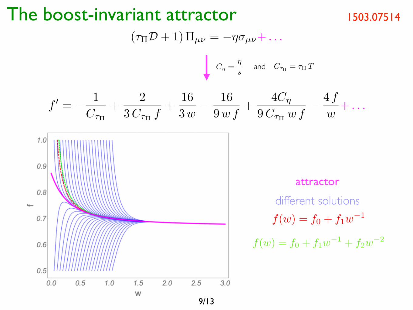
(⌧⇧D + 1)⇧µ⌫ = �⌘�µ⌫+ . . .

f 0 = � 1

C⌧⇧

+2

3C⌧⇧ f+

16

3w� 16

9w f+

4C⌘

9C⌧⇧ w f� 4 f

w+ . . .

C⌘ =⌘

sC⌧⇧ = ⌧⇧ Tand

attractor

f(w) = f0 + f1w�1

f(w) = f0 + f1w�1 + f2w

�2

different solutions

1503.07514

Gradient expansion

10/13

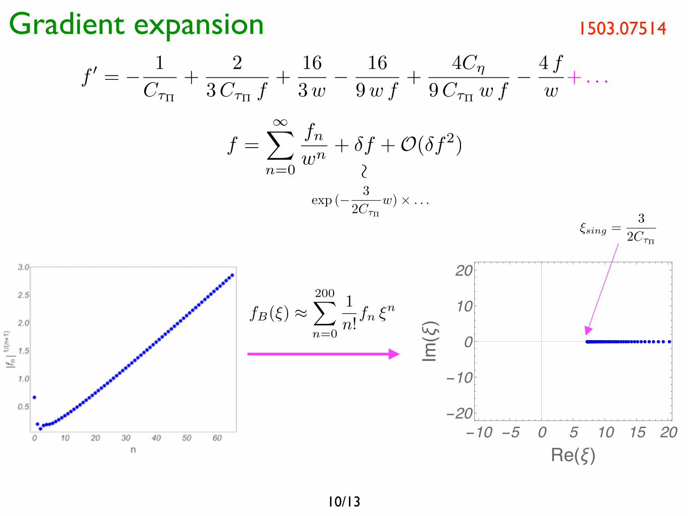
f 0 = � 1

C⌧⇧

+2

3C⌧⇧ f+

16

3w� 16

9w f+

4C⌘

9C⌧⇧ w f� 4 f

w+ . . .

f =1X

n=0

fnwn

+ �f +O(�f2)

⇠

exp (� 3

2C⌧⇧

w)⇥ . . .

fB(⇠) ⇡200X

n=0

1

n!fn ⇠

n =200X

n=0

fn ⇠n

-�� -� � � �� �� ��-��

-��

�

��

��

��(ξ)��

(ξ)

⇠sing =3

2C⌧⇧

1503.07514

Transseries

11/13

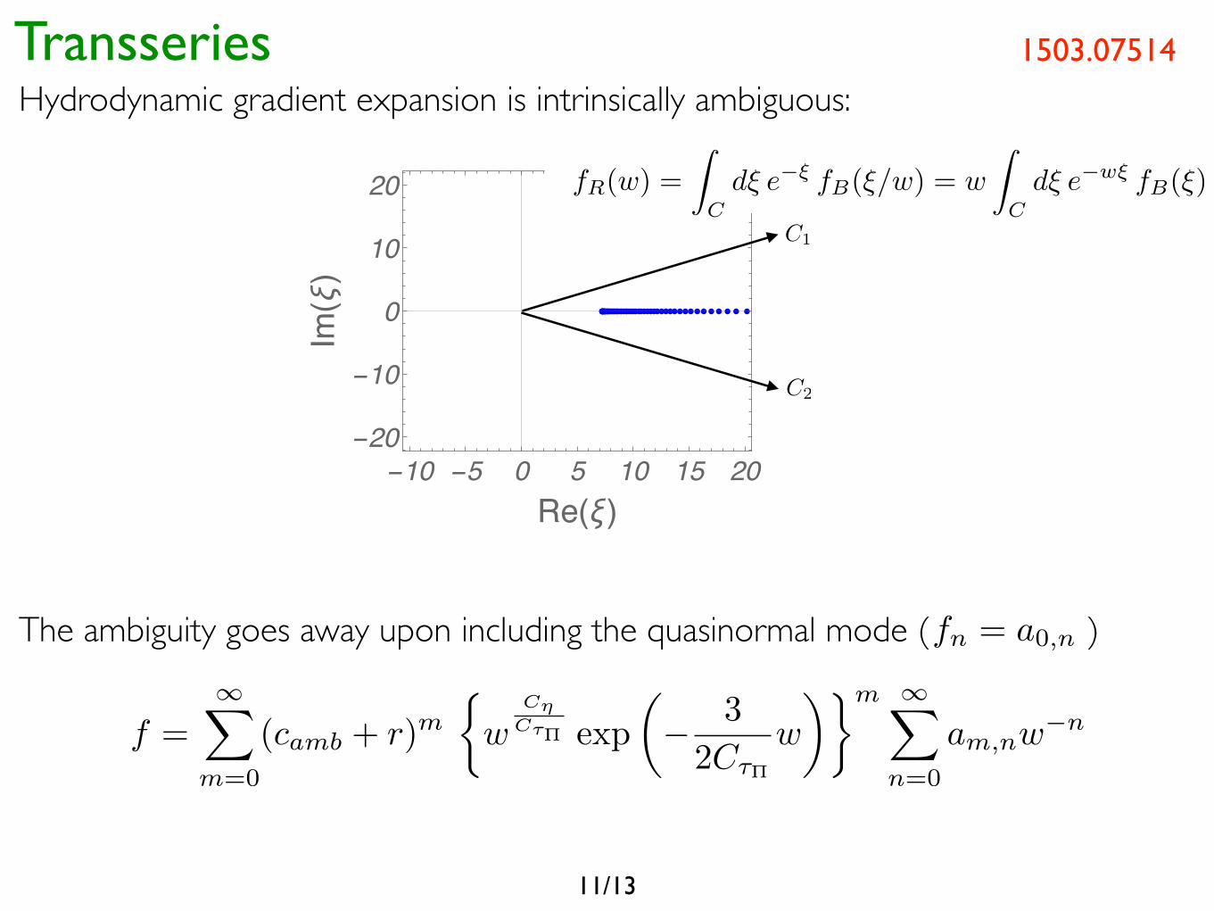
Hydrodynamic gradient expansion is intrinsically ambiguous:

-�� -� � � �� �� ��-��

-��

�

��

��

��(ξ)

��(ξ)

3

FIG. 1. The blue lines are numerical solutions of Eq. (9) forvarious initial conditions; the thick, magenta line is the nu-merically determined attractor. The red, dashed and green,dotted lines represents first and second order order hydro-dynamics. The upper plot was made with parameter valuesappropriate for N = 4 SYM, while the lower plot has both⌘/s and C⌧⇧ increased by a factor of 3. Note that in the lattercase the hydrodynamic attractor is attained at larger valuesof w, as expected from Eq. (12).

By setting the initial value of f at small w which is arbi-trarily close to Eq. (13), the attractor can be determinednumerically with the result shown in Fig. 1.

Another way of characterizing the attractor is to ex-pand Eq. (10) in derivatives of f – this is an analog of theslow-roll expansion in theories of inflation (see e.g. [19]).This way one generates a kind of gradient expansion, butthis is not the usual hydrodynamical expansion, sincethe generated approximations to f are not polynomialsin 1/w. By choosing the correct branch of the squareroot which appears at leading order one can ensure thatexpanding the k-th approximation in powers of 1/w one

finds consistency with hydro at order k + 1. At leadingorder one finds

f(w) =2

3� w

8C⌧⇧+

p64C⌘C⌧⇧ + 9w2

24C⌧⇧. (14)

Continuing this to second order gives an analytic repre-sentation of the attractor which matches the numericallycomputed curve even for w as small as 0.1. The slow-rollexpansion at low orders gives a very accurate representa-tion of the hydro attractor, but it is easily checked thatthis expansion is also divergent.Finally, one can also construct the attractor in an

expansion around w = 0 starting with f(w) given byEq. (13). It turns that the radius of convergence of thisseries is finite. All three expansion schemes describedabove – the expansion in powers of w, in powers of 1/wand the “slow-roll” expansion are consistent with the nu-merically determined attractor.

Hydrodynamic Gradient Expansion at High Orders.– Inwhat follows we focus on the hydrodynamic expansion,the expansion in powers of 1/w. It is straightforward togenerate the gradient expansion up to essentially arbi-trarily high order (in practice we chose to stop at 200).As seen in Fig. 2, the coe�cients fn of the series solution

f(w) =1X

n=0

fnw�n (15)

show factorial behaviour at large n. This is completelyanalogous to the results obtained in [6] for the case ofN = 4 SYM.In view of the divergence of the hydrodynamic expan-

sion we turn to the Borel summation technique. TheBorel transform of f is given by

fB(⇠) =1X

n=0

fnn!

⇠n (16)

and results in a series which has a finite radius of con-vergence. Note that in Eq. (16) large w corresponds tosmall ⇠. To invert the Borel transform it is necessary toknow the analytic continuation of series (16), which wedenote by fB(⇠). The inverse Borel transform

fR(w) =

Z

Cd⇠ e�⇠ fB(⇠/w) = w

Z

Cd⇠ e�w⇠ fB(⇠) (17)

where C denotes a contour in the complex plane connect-ing 0 and 1, is interpreted as a resummation of the orig-inal divergent series (15). To carry out the integration itis essential to know the analytic structure of fB(⇠).One way to perform the analytic continuation is to use

Pade approximants [20] which is the approach we adoptthroughout this study. We begin by examining the diago-nal Pade approximant given by a ratio of two polynomialsof order 100. This function has a dense sequence of poles

C1

C2

The ambiguity goes away upon including the quasinormal mode ( )

f =

1X

m=0

(camb + r)m⇢w

C⌘C⌧⇧

exp

✓� 3

2C⌧⇧

w

◆�m 1X

n=0

am,nw�n

fn = a0,n

1503.07514

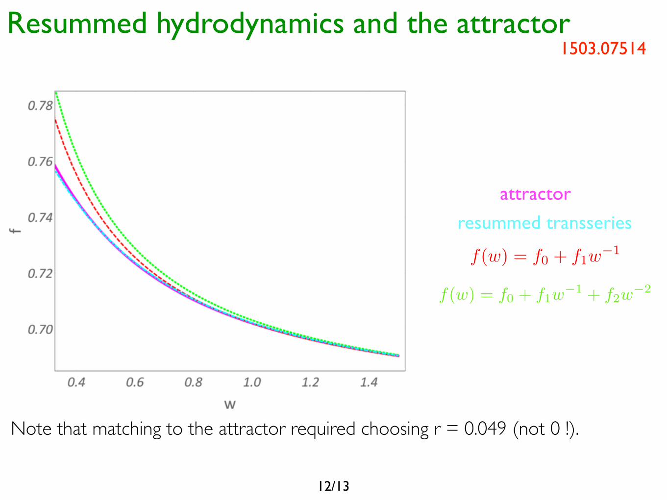
Resummed hydrodynamics and the attractor

attractor

resummed transseries

f(w) = f0 + f1w�1

f(w) = f0 + f1w�1 + f2w

�2

Note that matching to the attractor required choosing r = 0.049 (not 0 !).

12/13

1503.07514

Executive summary

1103.3452, 1302.0697, 1409.5087 & 1503.07514with R. Janik, M. Spaliński and P. Witaszczyk

Ab initio calculations in holography show that early applicability of viscoushydrodynamics in the presence of large gradients / large anisotropies is not crazy.

13/13