Metrology Prof. Dr. Kanakuppi Sadashivappa …...precise measuring tools. So, investment on...
21
Metrology Prof. Dr. Kanakuppi Sadashivappa Department of Industrial and Production Engineering Bapuji Institute of Engineering and Technology-Davangere Module-3 Lecture-4 Selection of fits, Geometrical tolerances (Refer Slide Time: 00:13) I, welcome you all for module 3 lecture 4. In this lecture we will be discussing about the various factors favouring the loose tolerances and tight tolerances. We will have the discussion on the selection of different kinds of fits and the assessment of the fit and tolerances. And how we can calculate the tolerance unit value also we will discuss about the geometrical tolerances. (Refer Slide Time: 00:55)
Transcript of Metrology Prof. Dr. Kanakuppi Sadashivappa …...precise measuring tools. So, investment on...

MetrologyProf. Dr. Kanakuppi Sadashivappa
Department of Industrial and Production EngineeringBapuji Institute of Engineering and Technology-Davangere
Module-3Lecture-4
Selection of fits, Geometrical tolerances
(Refer Slide Time: 00:13)
I, welcome you all for module 3 lecture 4. In this lecture we will be discussing about the various
factors favouring the loose tolerances and tight tolerances. We will have the discussion on the
selection of different kinds of fits and the assessment of the fit and tolerances. And how we can
calculate the tolerance unit value also we will discuss about the geometrical tolerances.
(Refer Slide Time: 00:55)

Now I am showing cube engineering parts, the bearings which require very fine finishes and very
tight tolerances. We can see here we have some bearings, ball bearings with very fine finish. So,
it is very essential that we have to control the dimensions. And it also necessary that we have to
control the features, geometric features . For example the roundness or flatness, straightness etc.,
etc.
So, that the function in a proper way. Here we have fluid film bearings used in hard disc. We can
see with have very fine finishes with very tight tolerances. So, that the function properly without
much run out a problem so, they require very fine IT grades like IT4, IT5 etc. So, that here
functioning will be proper.
(Refer Slide Time: 02:11)
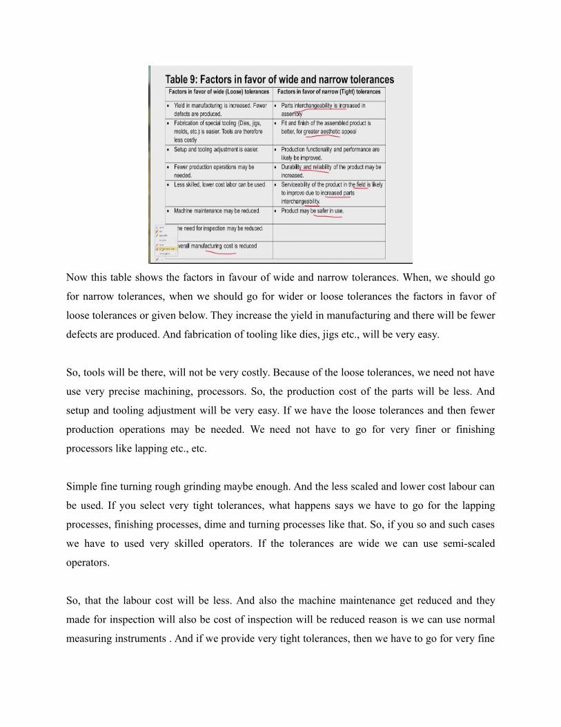
Now this table shows the factors in favour of wide and narrow tolerances. When, we should go
for narrow tolerances, when we should go for wider or loose tolerances the factors in favor of
loose tolerances or given below. They increase the yield in manufacturing and there will be fewer
defects are produced. And fabrication of tooling like dies, jigs etc., will be very easy.
So, tools will be there, will not be very costly. Because of the loose tolerances, we need not have
use very precise machining, processors. So, the production cost of the parts will be less. And
setup and tooling adjustment will be very easy. If we have the loose tolerances and then fewer
production operations may be needed. We need not have to go for very finer or finishing
processors like lapping etc., etc.
Simple fine turning rough grinding maybe enough. And the less scaled and lower cost labour can
be used. If you select very tight tolerances, what happens says we have to go for the lapping
processes, finishing processes, dime and turning processes like that. So, if you so and such cases
we have to used very skilled operators. If the tolerances are wide we can use semi-scaled
operators.
So, that the labour cost will be less. And also the machine maintenance get reduced and they
made for inspection will also be cost of inspection will be reduced reason is we can use normal
measuring instruments . And if we provide very tight tolerances, then we have to go for very fine
precise measuring tools. So, investment on inspection cost will increase if you have tight
tolerances.
And then overall manufacturing cost is reduced, reason is the not so precise machines can be
used and semi-scaled operators can be used and the inspection cost will reduced. So, due to these
the overall manufacturing cost also will reduce. And what are the conditions favouring tight
tolerances. So, when we provide very appropriate tight tolerances, the parts inter-changeability is
increased in assembly.
That means we can randomly select the mating parts and we can easily assemble. So, which may
not be possible, if the tolerances are very very loose and then fit and finish with their assembled
product will be better and the aesthetic appeal will also be better if you have tight tolerances.
And then production functionality and performance will be improved. And the products
produced will be durable and they will be reliable in service.
And the serviceability of the product in the field is likely to improve due to increased parts
interchangeable. That means the components to be replaced there readily available in the market.
Like bearings, belts etc., etc., tapper pins different kinds of fastener they are readily available.
So, we can purchase them and we can replace them. So, inter-changeability aspect will improve
and product will be safer to use.
(Refer Slide Time: 06:08)
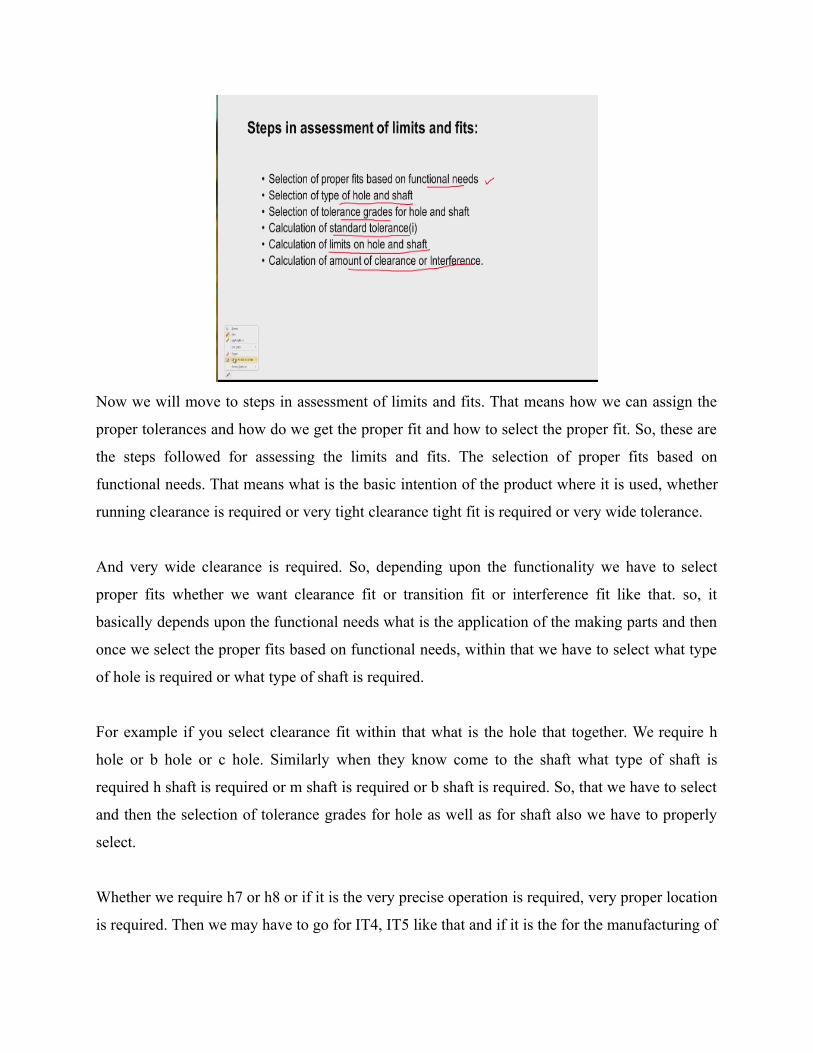
Now we will move to steps in assessment of limits and fits. That means how we can assign the
proper tolerances and how do we get the proper fit and how to select the proper fit. So, these are
the steps followed for assessing the limits and fits. The selection of proper fits based on
functional needs. That means what is the basic intention of the product where it is used, whether
running clearance is required or very tight clearance tight fit is required or very wide tolerance.
And very wide clearance is required. So, depending upon the functionality we have to select
proper fits whether we want clearance fit or transition fit or interference fit like that. so, it
basically depends upon the functional needs what is the application of the making parts and then
once we select the proper fits based on functional needs, within that we have to select what type
of hole is required or what type of shaft is required.
For example if you select clearance fit within that what is the hole that together. We require h
hole or b hole or c hole. Similarly when they know come to the shaft what type of shaft is
required h shaft is required or m shaft is required or b shaft is required. So, that we have to select
and then the selection of tolerance grades for hole as well as for shaft also we have to properly
select.
Whether we require h7 or h8 or if it is the very precise operation is required, very proper location
is required. Then we may have to go for IT4, IT5 like that and if it is the for the manufacturing of

gauges used for inspection purpose. We may have to go for IT2, IT3 like that. So depending
upon the again based upon the application we have to select proper tolerance grades for hole as
well as for shaft which will decide the amount of the tolerance on the hole and shaft.
And then we have to calculate the standard tolerance (i) for a particular combination. And then
calculation of limits on hole and shaft, that means once we know what is the type of hole and
what is the type of shaft. And then what is the tolerance grade we are using and after finding the
ta standard tolerance value. Then we can fix out what is the upper limit for the hole, what is the
lower limit for the hole.
And similarly what is the upper limit for shaft and what is the lower limit for the shafts. Those
things can be calculated and then after once we find the limits for hole and shaft, we can
calculate what is the amount of clearance what is the maximum amount of clearance what is the
minimum amount of clearance. If it is clearance fit and then we can if it is interference fit what is
the maximum interference, minimum interference.
And if it is transition fit what is the maximum interference what is the minimum clearance. Such
things can be calculated. And once we calculate all these things, so we can prepare the drawing
we can measure al the tolerance etc., etc., and that drawing can be supplied to the manufacturing
unit for the making of the products.
(Refer Slide Time: 09:52)
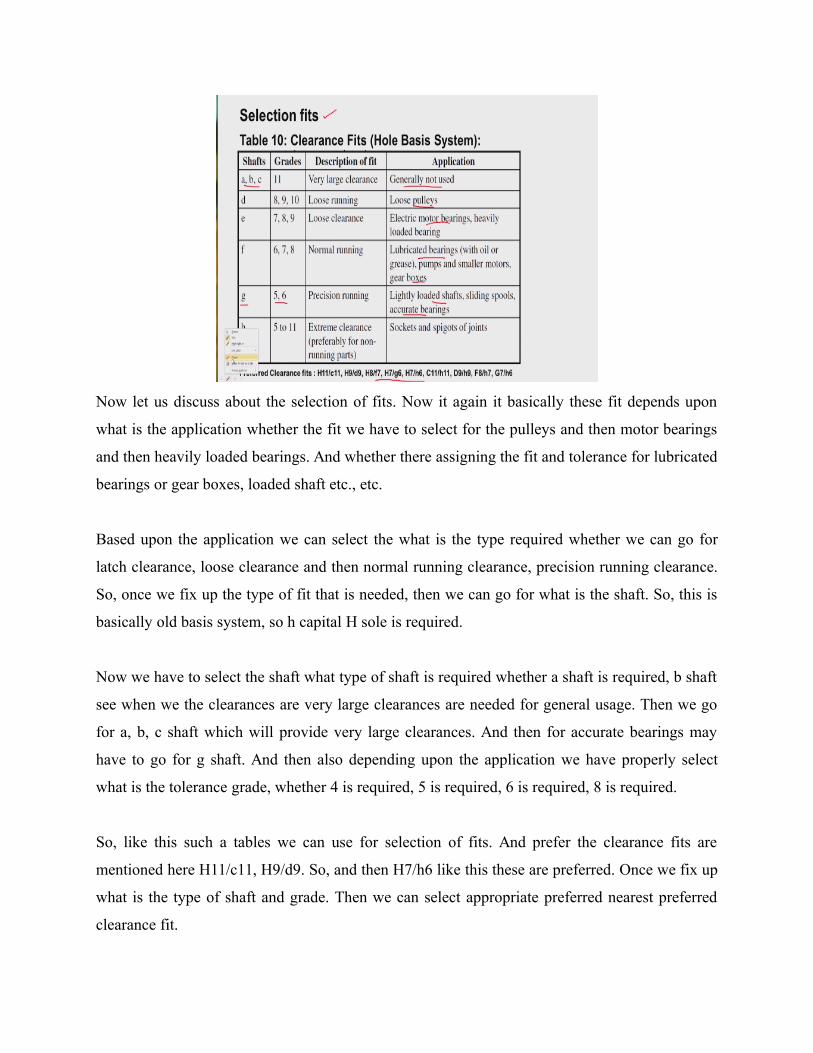
Now let us discuss about the selection of fits. Now it again it basically these fit depends upon
what is the application whether the fit we have to select for the pulleys and then motor bearings
and then heavily loaded bearings. And whether there assigning the fit and tolerance for lubricated
bearings or gear boxes, loaded shaft etc., etc.
Based upon the application we can select the what is the type required whether we can go for
latch clearance, loose clearance and then normal running clearance, precision running clearance.
So, once we fix up the type of fit that is needed, then we can go for what is the shaft. So, this is
basically old basis system, so h capital H sole is required.
Now we have to select the shaft what type of shaft is required whether a shaft is required, b shaft
see when we the clearances are very large clearances are needed for general usage. Then we go
for a, b, c shaft which will provide very large clearances. And then for accurate bearings may
have to go for g shaft. And then also depending upon the application we have properly select
what is the tolerance grade, whether 4 is required, 5 is required, 6 is required, 8 is required.
So, like this such a tables we can use for selection of fits. And prefer the clearance fits are
mentioned here H11/c11, H9/d9. So, and then H7/h6 like this these are preferred. Once we fix up
what is the type of shaft and grade. Then we can select appropriate preferred nearest preferred
clearance fit.
(Refer Slide Time: 12:07)
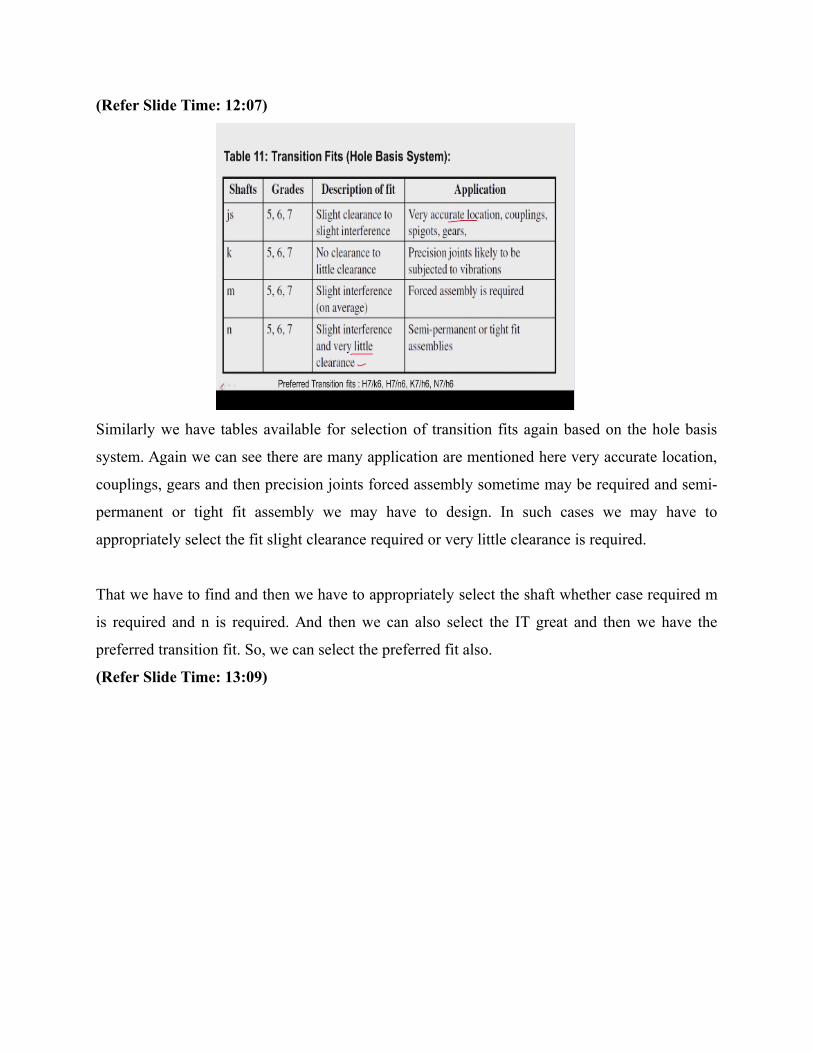
Similarly we have tables available for selection of transition fits again based on the hole basis
system. Again we can see there are many application are mentioned here very accurate location,
couplings, gears and then precision joints forced assembly sometime may be required and semi-
permanent or tight fit assembly we may have to design. In such cases we may have to
appropriately select the fit slight clearance required or very little clearance is required.
That we have to find and then we have to appropriately select the shaft whether case required m
is required and n is required. And then we can also select the IT great and then we have the
preferred transition fit. So, we can select the preferred fit also.
(Refer Slide Time: 13:09)

Similarly we have interference fit again some applications are mention here for fixing bushes.
We may go for interference fit for tight press fit and then valve seating and then permanent
assemblies. So, in such cases we go for interference fit for example for permanent assembly with
H capital H hole we can use the T shaft and U shaft. And for valve seatings collars etc... We can
go for S shaft with tolerance creates 5, 6 or 7.
And then again we have the preferred interference fits we can select the type of fit out of these
preferred interference fits.
(Refer Slide Time: 14:06)

Now after studying all these basics we will some numerical examples. I have taken an example
here we follow all the steps the for example selection of fit and calculation of tolerance unit etc.,
etc., so, that the basics can be understood clearly. Now the problem is the diameter of the shaft is
70 millimetre that is the basic size or the design size of the shaft is 70 millimetre. And then
tolerance grade is H8 for hole and f7 for shaft.
So, H hole with 80 8 grade is used and for shaft f shaft is used with 87 so, tolerance grades and
type of hole. They are already mention in the example now what we have to do is we have to
calculate the standard tolerance unit. And then whether there is any fundamental deviation and
then what is the upper limit and lower limit for shaft. Similarly what is the upper limit and lower
limit for hole that can be calculated and finally.
We can say whether the type of fit obtained is clearance fit or interference fit. Now we have to
find fundamental deviation tolerances for hole and shaft and limits of size for hole and shaft.
Also we have to mention what is the type of fit and also we have to calculate maximum and
minimum interference or maximum and minimum clearance depending upon fit obtain. We have
to mention what is maximum interference are clearance.
And what is maximum type maximum amount of these interferences and clearances, now we can
the solution is given here calculation of standard tolerance unit. So, we can use this equation i is
equal to 0.45 times cube root of D+0.001 times D so, where D is diameter mean diameter that
means we know that basic size is 70 millimetre. And then where it falls in what step it falls that
we have to see that we can do using table7 70mm.
It falls in the range of 52 to 80 now, we can find the mean D that is cube root of I am sorry
square root of 50 times 80. So, this will be equal to 63.25millimetre this is the value of mean
diameter now we have to insert this D in this equation to find the tolerance unit. So, the value of
D is inserted here 0.45 times cube root of 63.25+0.001 times 63.25. So this will give us 1.865
micrometre or 0.0018millimetre.

Now after finding this i we can find the tolerance values for shaft and hole now, we are using f7
shaft so, tolerance value for height is greater 7 is equal to 16i so, this we can get from table
number5. So, now tolerance value for the shaft is equal to 16 times i where i is equal to
0.0018millimetre so, this will be equal to 0.03millimetre. Similarly we can find the tolerance
value for hole, so where using H hole with it grade 8.
So, tolerance value for IT 8 will be 25i and then i value we have already calculated that is 0.0018
millimetre. So, tolerance for shaft I am sorry for tolerance for hole will be equal to 25i that will
be equal to 0.046millimetre.
(Refer Slide Time: 18:48)
Now after finding tolerance unit and tolerance values for hole and shaft we can find the
fundamental deviation since we are using hole basis system. The fundamental that is H hole we
are using so, fundamental deviation for hole is 0, now we have to find the fundamental deviation
for the shaft f. Now from the table number4 we can get this equation for getting the fundamental
deviation for f shaft.
So, for f shaft fundamental deviation that is upper deviation is equal to -5.5 times D to the power
of 0.41. So, we have to feed the value of D that is 63.25 then we get fundamental deviation
which is nothing but upper deviation as 0.030millimetre. So, once we find the fundamental
deviation tolerance value, we can fix up the limits for shaft and hole. Now higher limit for shaft
is equal to the basic size of the shaft that is 70millimetre –fundamental deviation.
So, that is 0.03 millimetres so, we get higher limit as 69.97millimetre similarly for lower limit of
the shaft higher limit of shaft–tolerance that is higher limit is 69.97. And the tolerance value for
the shaft is 0.03, so this will give as lower limit of 69. 94millimetre. Similarly for hole we can
find lower limit and upper limit, so in this case lower limit for hole is 70millimetre reason is
fundamental deviation is 0.
That means lower limit half the hole will be equal to basic size that is 70millimetre and higher
limit can be calculated by adding tolerance to the lower limit. So, we get 70.046millimetre. Now
we can show this graphically like this we have 0 line this is 0 line from this 0 line we show all
the other dimensions like tolerance value, basic size etc, etc... Now we are using H8 hole. So,
this is H8 and for H hole H8 hole, we have calculated the tolerance value.
So, tolerance for H hole is 0.046 millimetre that is this tolerance value is 0.046, 0.046
millimetres and then coming to the this is the lower limit for the hole which is equal to the basic
size 70millimetre. Since the deviation is 0 the lower limit for the hole is equal to the basic size
and we have to add this tolerance value to this basic size to get the upper limit of the hole then
upper limit of the hole is 70.046millimetre this is the upper limit.
Now we have f7 shaft so, this is f7 shaft with the tolerance value of tolerance value for f7 shaft is
30 microns. So, this is 0.03millimetre and also the fundamental deviation that is upper deviation.
So, upper limit of the shaft is nearer to the 0 lines so, this is upper deviation and we have
calculated the upper deviation for the shaft that is 0.03millimetre. Now using the tolerance value
and this upper deviation we can fix up the limits for the shaft.
So, that we have already found here year limit of the shaft, this is the higher limit h limit for
shaft. So, higher limit is 69.97 and then lower limit we get at this point. So, this gives us the
lower limit that means from the upper limit they have to detect this tolerance value. Then we
obtain the lower limit and so, this is the maximum clearance so this guess as the maximum
clearance that means to get the maximum clearance.
When the shaft size is equal to the lower limit, and the hole size is equal to the maximum, then
we get the maximum clearance maximum. So, what we have to do is we have to add this
tolerance for shaft and then we have to add this fundamental deviation. And then we have to add
this tolerance for hole then we get the maximum clearance, and this difference between the
minimum size of the hole. And maximum size of the shaft will give as the minimum clearance
that is equal to 0.03mm.
(Refer Slide Time: 26:15)
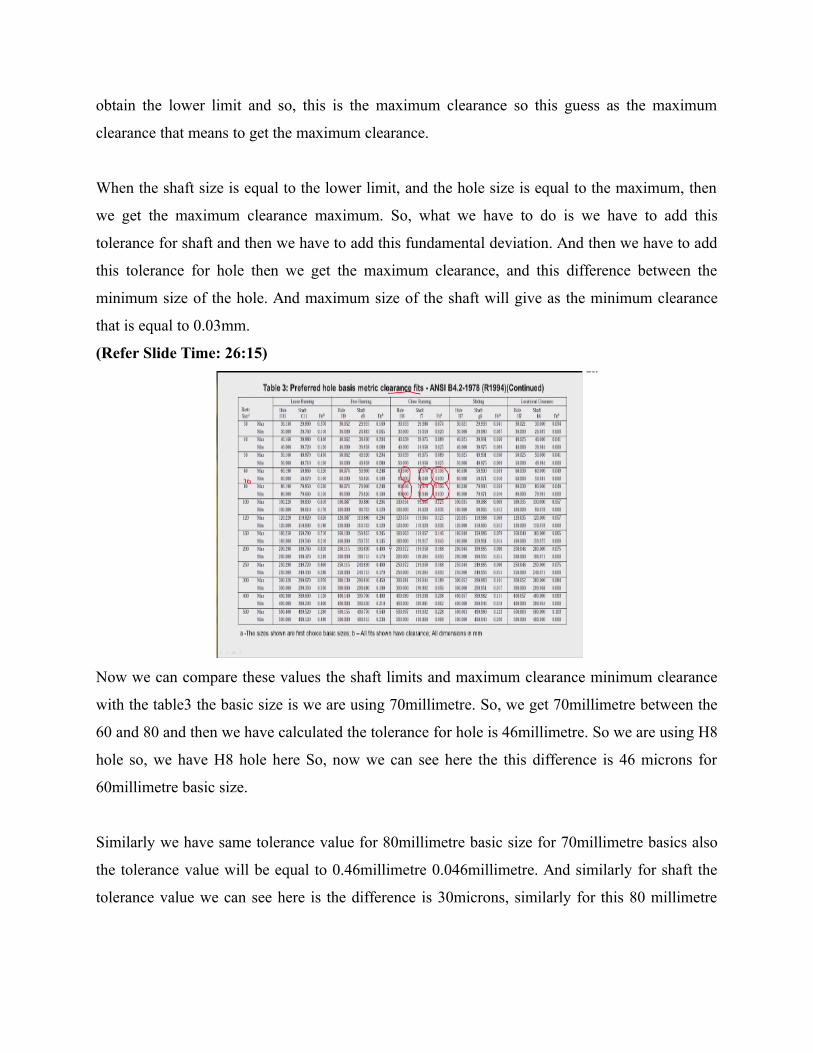
Now we can compare these values the shaft limits and maximum clearance minimum clearance
with the table3 the basic size is we are using 70millimetre. So, we get 70millimetre between the
60 and 80 and then we have calculated the tolerance for hole is 46millimetre. So we are using H8
hole so, we have H8 hole here So, now we can see here the this difference is 46 microns for
60millimetre basic size.
Similarly we have same tolerance value for 80millimetre basic size for 70millimetre basics also
the tolerance value will be equal to 0.46millimetre 0.046millimetre. And similarly for shaft the
tolerance value we can see here is the difference is 30microns, similarly for this 80 millimetre

size that is tolerance value is 30micrometre 0.03mm. So, for 70 also same value will be there and
then we can also see the maximum clearance and minimum clearance.
All these are clearance fits you can see minimum clearance is 0.03 millimetre and maximum
clearance is 0.106 millimetre that we can observe here minimum clearance is 0.03 millimetre and
maximum clearance is 0.106 millimetre like this we can calculate the values or if ready tables are
available, we can use the ready table to get the to fix up the limits for hole and shaft and to get
the type of fit.
(Refer Slide Time: 28:28)
Now we have a special case of 3 lobe now in all the previous examples, what we studied is based
upon the hole size and the shaft size. We get particular type of fit it means if shaft is smaller than
the hole we get clearance fit, if the shaft is greater than the hole. Then we get the interference fit
and sometimes we get transition fit depending upon the actual size of the hole and shaft if the
tolerance zones are overlapping.
Now this fit can we calculated by measuring the actual sizes of hole and shaft or if we know the
tolerance zone for hole and shaft. We can we come to know whether we get it clearance fit or
interference fit wet sometimes what happens is the shaft will not be circular that means we may
get some lobes like this. So, this happens normally in centralise grinding varying we have
supporting role.

And then we have the work piece and then we have rest blade2 keep the work pieces and then we
have the grinding wheel. So, if the work piece setting is not proper or the blade height is not set
properly. Then there are chances let we may get the some errors like this you may get lobed
shafts now if may measure this diameter using a micrometre that means 2 point contact method.
Everywhere it gives same value it so micrometre measurement will not give us whether there is
any lobbing or not. If it is elliptical shape it gives the difference we can find fine the maxi this is
minimum diameter and maximum diameter. Then we can find at there is any different we can
find that there is lobe ovalities there. But for 3 lobe the micrometre measurement will not
indicate, whether there is any 3 lobe or not.
So, we just measured the diameter and we measure the diameter the hole and then we try to we
calculate the type of fit what happens is say we have a diameter of hole is a 20.02millimetre.
This is the diameter of the hole and then we have micrometre measurement gives that the
diameter of shaft is say 20.030millimetre. So, this is the diameter of the shaft obtain by
micrometre then what we can conclude is the diameter the shaft is greater than the diameter of
the holes.
So, immediately we say that the fit type of fit what we are going to get is interference fit. But in
actual practice when we try to insert this 3 lobed shaft into the hole it will entered. So, how this
is possible see now we try to insert this so, this is the centre of the hole oven and then this is
centre of the shaft o2. Now when both the centres coincide then the situation will be like this that
means o2 is coinciding with oven then there will be interference.
But in actual practice what happens is we have this circle with oven centre, and then we try to
insert this is now you can see re is some clearance. So what happens is the shaft will move down
and then it will enter into the hole so situation will be like this. And o2 will be somewhere here.
So actually we get instead of getting interference fit as per the measurement. We get the
clearance fit in actual practice.

So, we should be careful in getting the fits that means near dimensional measurement or the
specification of dimensional tolerance for hole and shaft is not enough. We have to specify the
geometrical tolerance also. So what is the amount of error that can be allowed on the straightness
or flatness or roundness or cylindricity. So, geometrical tolerance is also very very important to
get proper type of fit and for proper functioning.
(Refer Slide Time: 34:09)
See now we will have discussion on geometrical tolerance now you can see here the straightness
of an edge say we have line like this. So we have line like this but in actual practice we may
measure it may be like this. So, it will vary the points will vary of course the gap will be very
small it will be in terms of few microns. So, now it is very difficult to machine a perfect straight
edge.
So, we have to allow some tolerance for the straightness and then that we can do by specifying
what is the gap between these two lines say it may be some like 0.01millimetre or 0.02millimetre
like the depending upon the application. So, straightness is also specify on the drawings, so it is
to control straightness of a line or axis or a surface. So, basically it is gap between two parallel
straight lines in a plain containing the consider line.
That means the line may be like this and what is the maximum deviation on straightness that is
allow. So, that is mention like 0.01, 0.02 etc. So, now the single used for specifying the so, we

have cylinder like this and will be having so many generators. And we want the straightness of
this should not exceed say 0.03 so, we have to specify like this. So, straightness symbol is a short
line and then we have to specify, what is the value.
Whether it is 0.01millimetre or 0.02millimetre so, that value this is the tolerance value and this is
the feature straightness this for straightness this like this we specify the straightness. Similarly
we can specify the flatness. So we have a surface like this for example the guide way of later any
machine tool. And you should be flat it is necessary that you should be straight as well as you
should be flat. So, that we can specify using this symbol flatness symbol like this
So, we have to specify the, what is the feature flatness in this case. And then we have to give
what is the value whether it is 0.02millimetre or 0.01millimetre like that. So, this is how we
specify the flatness it is basically to control the surface flatness and it is area between two plains
so, we have two plains here and the surfacing question say this is the surfacing question all there
are many high points and low points on the surface.
All the high points and low points should be contain within these two plains which are separated
by the given tolerance value. In this case 0 02millimetre now similarly we can we specify the
roundness what is the roundness that is allow it is basically to control secularity error in the plain
in which it place. And then how it is specify we use two concentric circles so, that area between
two concentric circles gives us the roundness.
That means so we have shaft which is necessary that it should be round but in practice there will
be some variations low points and high points will be there. All the low points and high points on
that particular round part should be should lay within these two circles. So, this value is mention
what is the amount of tolerance that is allowed whether it is 0.01 or 0.02 like that.
That value is mention and we specify the roundness like this. We use that symbol and then we
give the value, so this is how we specify the roundness.
(Refer Slide Time: 39:05)
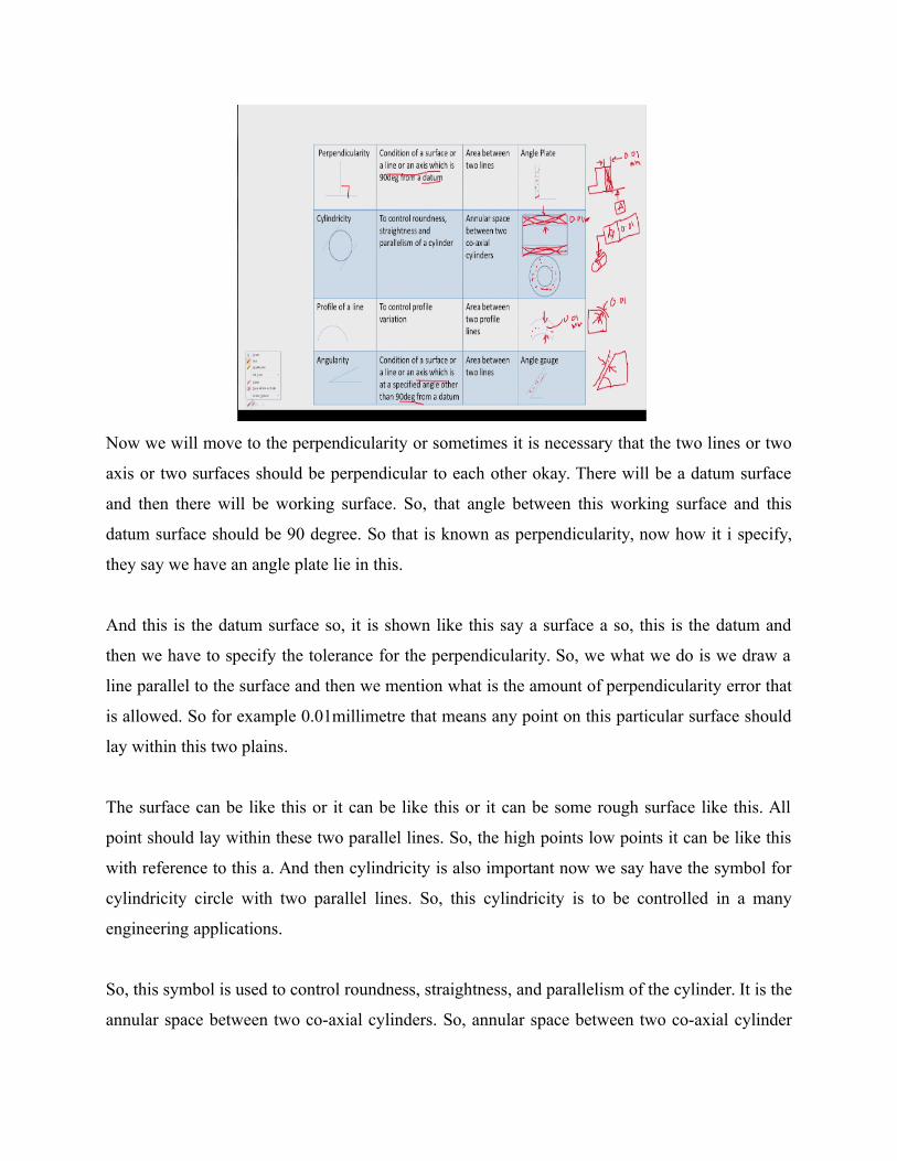
Now we will move to the perpendicularity or sometimes it is necessary that the two lines or two
axis or two surfaces should be perpendicular to each other okay. There will be a datum surface
and then there will be working surface. So, that angle between this working surface and this
datum surface should be 90 degree. So that is known as perpendicularity, now how it i specify,
they say we have an angle plate lie in this.
And this is the datum surface so, it is shown like this say a surface a so, this is the datum and
then we have to specify the tolerance for the perpendicularity. So, we what we do is we draw a
line parallel to the surface and then we mention what is the amount of perpendicularity error that
is allowed. So for example 0.01millimetre that means any point on this particular surface should
lay within this two plains.
The surface can be like this or it can be like this or it can be some rough surface like this. All
point should lay within these two parallel lines. So, the high points low points it can be like this
with reference to this a. And then cylindricity is also important now we say have the symbol for
cylindricity circle with two parallel lines. So, this cylindricity is to be controlled in a many
engineering applications.
So, this symbol is used to control roundness, straightness, and parallelism of the cylinder. It is the
annular space between two co-axial cylinders. So, annular space between two co-axial cylinder
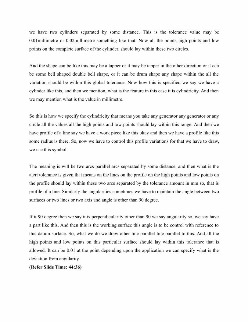
we have two cylinders separated by some distance. This is the tolerance value may be
0.01millimetre or 0.02millimetre something like that. Now all the points high points and low
points on the complete surface of the cylinder, should lay within these two circles.
And the shape can be like this may be a tapper or it may be tapper in the other direction or it can
be some bell shaped double bell shape, or it can be drum shape any shape within the all the
variation should be within this global tolerance. Now how this is specified we say we have a
cylinder like this, and then we mention, what is the feature in this case it is cylindricity. And then
we may mention what is the value in millimetre.
So this is how we specify the cylindricity that means you take any generator any generator or any
circle all the values all the high points and low points should lay within this range. And then we
have profile of a line say we have a work piece like this okay and then we have a profile like this
some radius is there. So, now we have to control this profile variations for that we have to draw,
we use this symbol.
The meaning is will be two arcs parallel arcs separated by some distance, and then what is the
alert tolerance is given that means on the lines on the profile on the high points and low points on
the profile should lay within these two arcs separated by the tolerance amount in mm so, that is
profile of a line. Similarly the angularities sometimes we have to maintain the angle between two
surfaces or two lines or two axis and angle is other than 90 degree.
If it 90 degree then we say it is perpendicularity other than 90 we say angularity so, we say have
a part like this. And then this is the working surface this angle is to be control with reference to
this datum surface. So, what we do we draw other line parallel line parallel to this. And all the
high points and low points on this particular surface should lay within this tolerance that is
allowed. It can be 0.01 at the point depending upon the application we can specify what is the
deviation from angularity.
(Refer Slide Time: 44:36)

Similarly we have the symbol for parallelism say we have work piece like this. And then this top
surface should be parallel to this datum. Datum is shown like this so, this is the datum say a, a
surface is datum. And all the points on this particular surface or line should lay within these two
lines which are separated arcs surfaces separated by the given amount of tolerance. For example
0.01mm high points and low points.
All should lay within these two lines or two planes now how this is designated. So, it is shown
like this we have to use the parallelism symbol and then we have to give the value what is the
tolerance that is alone. And then we have to specify datum with reference to which plane they
should be parallel. So, that reference or datum surface also we have to specify and then we have
another feature concentricity say we have two steps damper steps like as shown here.
And then the axis of this particular part should be concentric with the axis of the other part. So,
and if there is any deviation then what is the amount of deviation okay that is indicated by using
two circles concentric circles. And that is specified like this so, we have this is the reference
datum say this is A, surface A okay and then this axis should be parallel to this or concentric with
this within the certain tolerance.
So, we specify like this, this is the symbol feature symbol for concentricity, and then we have to
specify what is the tolerance. And then we have to specify with reference to which reference or

datum like this we specify the concentricity. And then similarly profile of a surface sometimes
we need to control the profile of a surface. So, in that case what we do is we use this particular
symbol the meaning of this is the we have to surfaces two surfaces like this separated by the
given tolerance amount.
For example 0.01millimetre okay all the points on the profile surface should lay within these two
surfaces separated by the given amount of tolerance. So now how to specify the profile tolerance
is shown here, we have to use this symbol and then we have to mention what is the deviation that
is allowed. Now in this lecture we discussed about the various aspects like selection of fits
calculation of tolerance unit value.
And then what are the factors favouring loose tolerances and tight tolerances, we also discussed
about the various geometrical tolerances for geometrical features. In the next class we will be
discussing about the various positional tolerances, how to specify positional tolerance and then
we will also say some numerical problems.