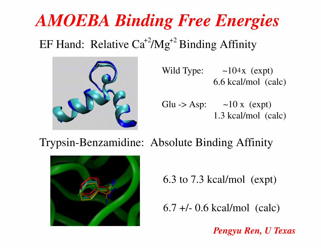
Methods for Free Energy Calculations

CHEM 430

Why Do This?• The free energy of a system is perhaps the most

important thermodynamic quantity, and is usually taken as the Helmholtz or Gibb’s free energy

• Techniques to calculate the free energy (or relative free energy) of a system are very useful studying phase transitions, critical phenomena or other transformations

• We can never calculate absolute free energies (since we don’t have an appropriate reference state), however relative free energies can be found using several different computational techniques

Calculating Free Energies• We know from statistical mechanics that we can

calculate the free energy (here the Helmholtz free energy) by evaluating integrals like

where H is the Hamiltonian.

• In practice it is very difficult to evaluate such integrals using MC or MD since we do not adequately sample high energy regions

A = kBT ln!""

dpNdrN exp#−βH(pN , rN )

$%

∆A = −kBT ln

&''dpNdrN exp

#−βHY (pN , rN )

$''

dpNdrN exp [−βHX(pN , rN )]

(

Calculation of Free Energy Differences• Although our simulation methods cannot

give us absolute free energies, free energy differences are much more tractable

• Consider two states X and Y

• Since the free energy is a state function, the difference in energy between these two states is simply

∆A = −kBT ln!''

dpNdrN exp [−βHY ] exp [βHX ] exp [−βHX ]''dpNdrN exp [−βHX ]

%

= −kBT ln!''

dpNdrN exp [−β(HY − HX)] exp [−βHX ]''dpNdrN exp [−βHX ]

%

Free Energy Differences• If we multiply the numerator by the factor

we getexp(βHX) exp(−βHX) ≡ 1

Free Energy Difference• Since we are clever, we notice that this is

nothing more than an ensemble average taken over the state X

• Equivalently we could write the reverse process

∆A = −kBT ln⟨exp [−β(HY − HX)⟩X

∆A = −kBT ln⟨exp [−β(HX − HY )⟩Y

Overlapping States• In order to evaluate an ensemble average

like

we could run a simulation either state X or Y and collect statistics

• Problems arise however when the states X and Y do not overlap such that simulating one state does a poor job of sampling the other

∆A = −kBT ln⟨exp [−β(HY − HX)⟩X

Intermediate States• If the energy difference between the two

states is large

we can introduce an intermediate state between X and Y

∆A = A(Y ) − A(X)= (A(Y ) − A(I)) + (A(I) − A(X))

= −kBT ln)Q(Y )Q(I)

× Q(I)Q(X)

*

|HX − HY | ≫ kBT

Intermediate States• We can obviously extend this treatment to

include multiple intermediate states with increasing overlap

∆A = A(Y ) − A(X)= (A(Y ) − A(N)) + (A(N) − A(N − 1)) + · · ·+ (A(2) − A(1)) + (A(1) − A(X))

= −kBT ln)

Q(Y )Q(N)

× Q(N)Q(N − 1)

· · · Q(2)Q(1)

× Q(1)Q(X)

*

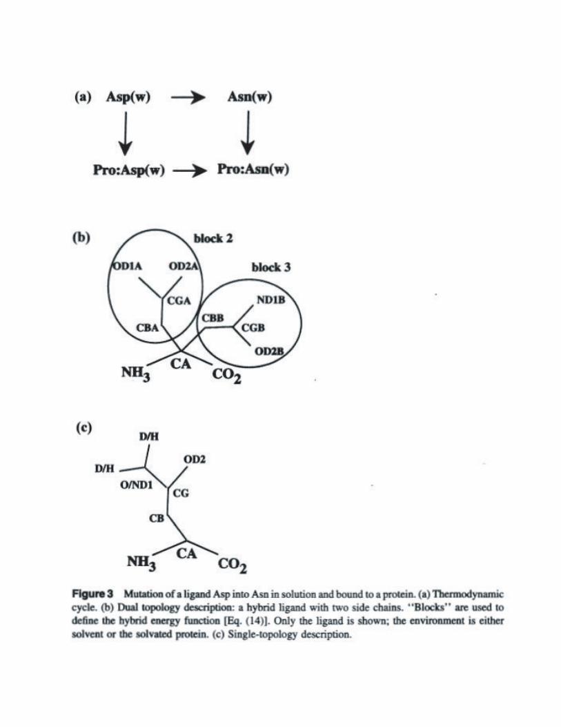
Intermediate States• One key to this method is that

intermediate states do not need to correspond to actual physical states (consider changing ethane to ethanol)

• Using molecular mechanics we can smoothly interpolate between these two states

H C

H

H

C

H

H

H C

H

H

C

H

H

H O H

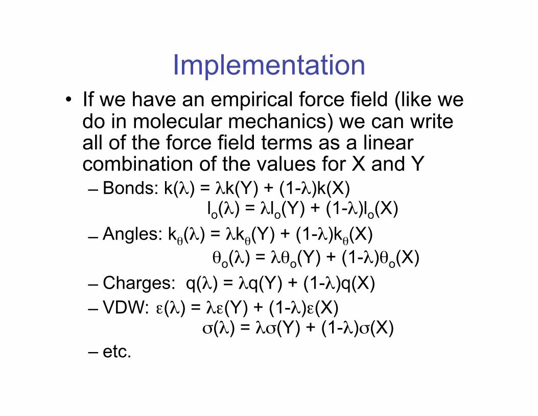
Implementation• If we have an empirical force field (like we

do in molecular mechanics) we can write all of the force field terms as a linear combination of the values for X and Y– Bonds: k(�) = �k(Y) + (1-�)k(X)

lo(�) = �lo(Y) + (1-�)lo(X)– Angles: k�(�) = �k�(Y) + (1-�)k�(X)

�o(�) = ��o(Y) + (1-�)�o(X)– Charges: q(�) = �q(Y) + (1-�)q(X)– VDW: �(�) = ��(Y) + (1-�)�(X)

�(�) = ��(Y) + (1-�)�(X)– etc.

∆A(λi → λi+1) = kBT ln⟨exp(−β∆Hi)⟩

Coupling Parameter• As we change the coupling parameter �

from 0 to 1, we move from state X to Y• At each intermediate step �i we perform a

simulation (Monte Carlo or MD) by first performing a short equilibration run (since our point of equilibrium has changed) and then a “production” run where we calculate

Free Energy Perturbation

0 1�

��(�

���

i+1)

�A

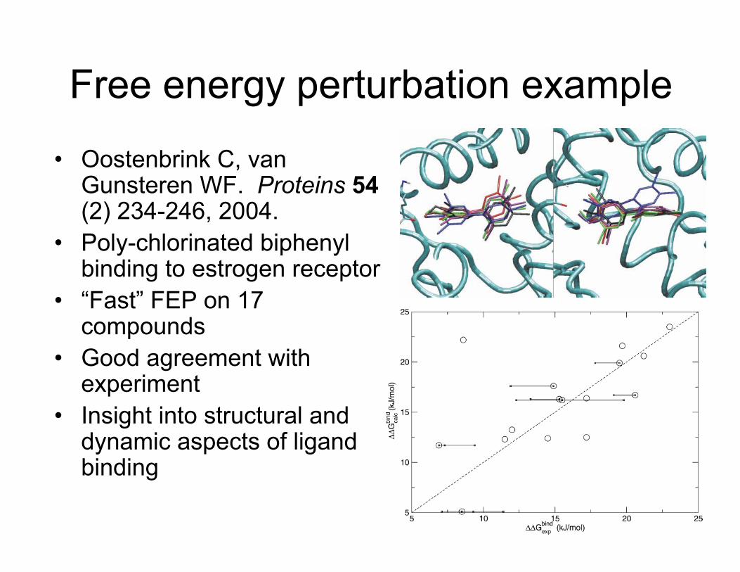
Free energy perturbation example

• Oostenbrink C, van Gunsteren WF. Proteins 54 (2) 234-246, 2004.

• Poly-chlorinated biphenyl binding to estrogen receptor

• “Fast” FEP on 17 compounds

• Good agreement with experiment

• Insight into structural and dynamic aspects of ligand binding

3 3

6.

−2 0 2 4

Change in Binding Energy (kcal/mol)

0

0.1

0.2

0.3

0.4

0.5

0.6

0.7

Pro

bab

ilit

y o

f S

yn

thesis

of

Co

mp

ou

nd

Original Distribution

Screen with 0.5 kcal/mol errorScreen with 1.0 kcal/mol errorScreen with 2.0 kcal/mol error1.4 kcal/mol Improvement

Error Analysis for Binding Energy Prediction

SAMPL5CBClip Host

● All CBClip binding experiments were performed at pH = 7.4 in 20mM sodium phosphate buffer

● Experimental values via UV-VIS and NMR competition assays

● Absolute FE binding computed with AMOEBA via a restrained double decoupling protocol

NH3 NH3G1p-Xylylenediamine

G2Putrescine

G3Spermine

G5Acridine Orange

G6(X = NHMe )2

G4Proflavine

G9NeutralRed

G7(X = CO )2

G10MethyleneBlue

NH3

NH3

H3N

H2N

NH2

NH3

N NH2H2N N NMe2Me2N

NH

N

NMe2H2N

Me

S

N

NMe2Me2N

NEt2

NEt2

N N

O

O

O

O

XX G8Brilliant Green

SAMPL5 CBClip Guests

SAMPL5 CBClip Binding Results

2

3

7

6

5

10

9

4

8

1

Cal

cula

ted Δ

G (

kcal

/mol

)

Experimental ΔG (kcal/mol)-12 -10 -8 -6 -4 -2 0

0

-2

-4

-6

-8

-10

-12

Avg Error = 0.94RMS Error = 1.13Pearson R = 0.90

Black Bars arepKa Corrections

Attomolar CB7 Host-Guest Binding

Experiment: -23.66 (Fluorescence / NMR)

-24.35 (ITC + Competition)Calculated: -24.26 (AMOEBA / BAR / > 5μs)

(kcal/mol)-20.86 (50 mM NaOAc, pH 4.7)(+/- 0.2)

(+/- 0.1)

Thermodynamic Integration• Instead of evaluating the difference in the

free energy between subsequent states, we could also calculate the derivative of the Hamiltonian

• In this case, the free energy difference is the area under the curve

∆A =" λ=1

λ=0

+∂H

∂λ

,

λ

dλ

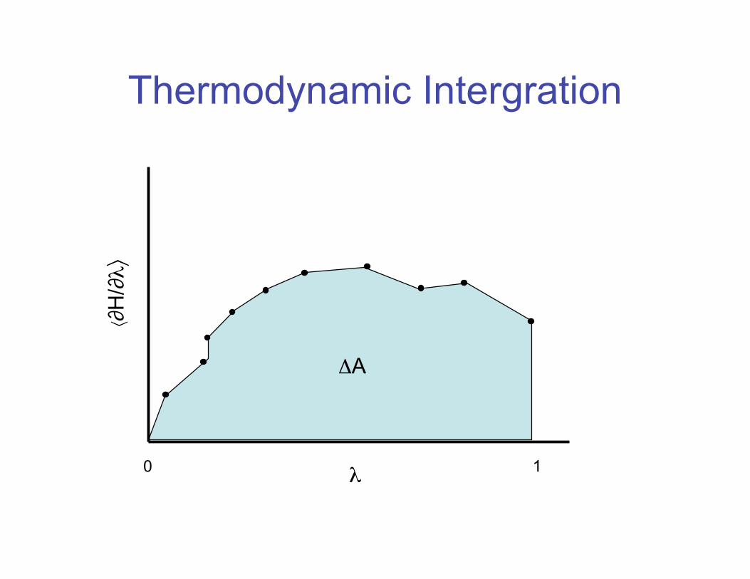
Thermodynamic Intergration

0 1�

��H

/���

�A

∆A = −kBT-

ln ⟨exp (−β [H(λi+1) − H(λi)])⟩

≃ −kBT-

ln ⟨1 − β [H(λi+1) − H(λi)]⟩

≃-

[H(λi+1) − H(λi)]

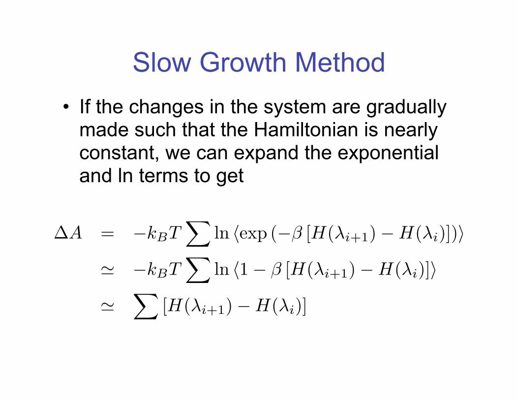
Slow Growth Method• If the changes in the system are gradually

made such that the Hamiltonian is nearly constant, we can expand the exponential and ln terms to get

More Reading• Many references and papers that cover

these topics. In the texts for this class consider:– Leach Chapter 11 (watch for errors!!)– Frenkel & Smit Chapter 7

Umbrella Sampling andHistogram Methods

The Sampling Problem• By now you realize that the major problem in

simulations is that of sampling• We have an exact method of computing a

partition function and associated thermodynamic quantities, however this is dependent on us accurately sampling the entire conformational space

• In general (i.e. the way most people run simulations) MD simulations do not do an adequate jobs of sampling configurational space unless run for a very, very long time

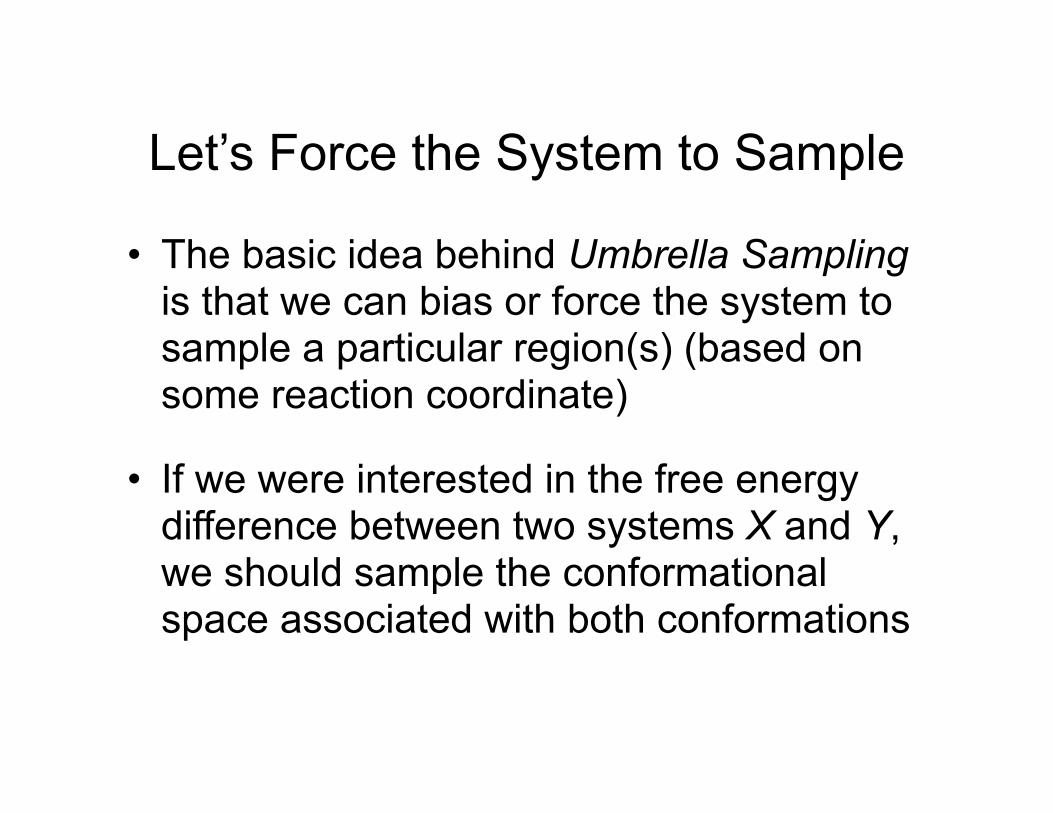
Let’s Force the System to Sample

• The basic idea behind Umbrella Sampling is that we can bias or force the system to sample a particular region(s) (based on some reaction coordinate)

• If we were interested in the free energy difference between two systems X and Y, we should sample the conformational space associated with both conformations

Free Energy Perturbation• Recall from our discussion of FEP that the free energy

difference between two systems can be expressed as

or equivalently

∆U = −kBT ln!''

drN exp [−βUY ]''drN exp [−βUx]

%

⟨exp(−β∆U)⟩X =''

drN exp [−βUY ]''drN exp [−βUx]

A New Weight Function• In order to sample both X and Y spaces, we now

introduce a new weight function �(rN) to replace the Boltzmann factor

which using our shorthand notation becomes

⟨exp(−β∆U)⟩X =''

drNπ(rN ) exp [−βUY ] /π(rN )''drNπ(rN ) exp [−βUx] /π(rN )

⟨exp(−β∆U)⟩X =⟨exp(−βUY )/π(rN )⟩π⟨exp(−βUX)/π(rN )⟩π

Umbrella Sampling Considerations• In order that both the numerator and

denominator are non-zero, the weight function �(rN) should have considerable overlap between the spaces of X and Y

• This property gives rise to the name Umbrella Sampling

• Although it appears we could sample the entire space with a single choice of �(rN), this is not optimal. It is still best to perform several sampling runs using overlapping windows

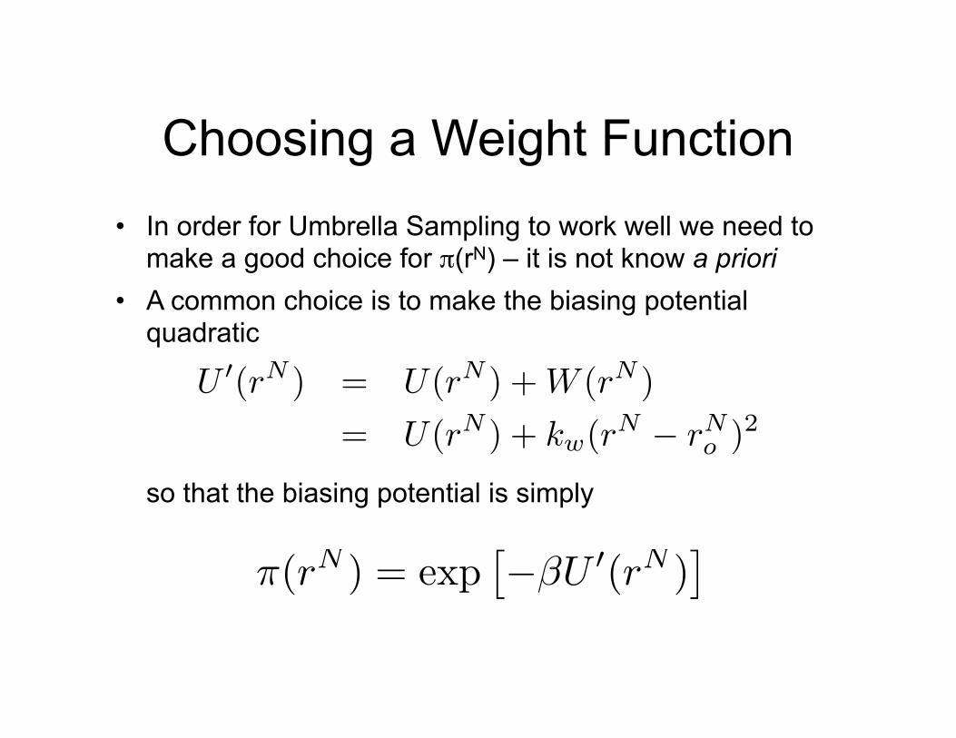
Choosing a Weight Function• In order for Umbrella Sampling to work well we need to

make a good choice for �(rN) – it is not know a priori• A common choice is to make the biasing potential

quadratic

so that the biasing potential is simply

U ′(rN ) = U(rN ) + W (rN )= U(rN ) + kw(rN − rN

o )2

π(rN ) = exp#−βU ′(rN )

$

Weighted Histogram Analysis Method (WHAM)

• Umbrella Sampling is valid in theory, but the implementation is often difficult since the “windows” of overlap must be carefully chosen to minimize the error (since the errors from the individual simulations add quadratically)

• WHAM is a useful method for combining sets of simulations with different biasing potentials in a manner such that the unbiased potential of mean force (PMF) can be found

Periodic Box Simulation (alanine dipeptide and 206 water molecules) Stochastic Dynamics

(576 trajectories of 200 picoseconds each) Free Energies via Umbrella Sampling and 2D-WHAM:

∑

∑

=

−−

== Nw

i

TkFwi

Nw

iwi

bii

i

en

n

1

/)),(

1),(

),(ψφ

ψφρψφρ

−= ∑∑ − ),(ln /),( ψφρ

ψ

ψφ

φ

Tkwbi

bieTkF

),(ln),( ψφρψφ TkG b−=∆

-180

-120

-60

0

60

120

180

-180 -120 -60 0 60 120 180

Psi

Phi

OPLS-AA

-180

-120

-60

0

60

120

180

-180 -120 -60 0 60 120 180

AMBER ff99

-180

-120

-60

0

60

120

180

-180 -120 -60 0 60 120 180

CHARMM27

3.22.82.42

1.61.20.80.4

Solvated AlanineDipeptide

Free EnergySurfaces

Examples and Further Reading

• Leach has some details on Umbrella Sampling in Ch. 11

• Frenkel & Smit discusses Umbrella Sampling and WHAM (disguised as the self-consistent histogram method) in Ch. 7

• There are many papers using these methods. (See Ron Levy paper that uses both techniques)