LUND UNIVERSITY

PO Box 117221 00 Lund+46 46-222 00 00

Methodological improvements in quantitative MRI

Perfusion estimation and partial volume considerationsAhlgren, André

2017

Link to publication

Citation for published version (APA):Ahlgren, A. (2017). Methodological improvements in quantitative MRI: Perfusion estimation and partial volumeconsiderations. Lund: Lund University, Faculty of Science, Department of Medical Radiation Physics.

General rightsUnless other specific re-use rights are stated the following general rights apply:Copyright and moral rights for the publications made accessible in the public portal are retained by the authorsand/or other copyright owners and it is a condition of accessing publications that users recognise and abide by thelegal requirements associated with these rights. • Users may download and print one copy of any publication from the public portal for the purpose of private studyor research. • You may not further distribute the material or use it for any profit-making activity or commercial gain • You may freely distribute the URL identifying the publication in the public portal

Read more about Creative commons licenses: https://creativecommons.org/licenses/Take down policyIf you believe that this document breaches copyright please contact us providing details, and we will removeaccess to the work immediately and investigate your claim.

Faculty of Science, Department of Medical Radiation Physics

ISBN 978-91-7753-098-5

978

9177

5309

85

An

dr

é Ah

lgr

en

Methodological im

provements in quantitative M

RI 2017

Methodological improvementsin quantitative MRIPerfusion estimation and partial volume considerations

André Ahlgren

depArtment of medicAl rAdiAtion physics | lund university 2017

Printed by Media-Tryck, 2017 | N

ordic Eco

label 3

041 0

903

Methodological improvements in quantitative MRI

Methodological improvementsin quantitative MRI

Perfusion estimation andpartial volume considerations

by André Ahlgren

esis for the degree of Doctor of Philosophyesis advisors: Linda Knutsson, Ronnie Wirestam and Freddy Ståhlberg

Faculty opponent: Associate Professor Michael Chappell, Institute of BiomedicalEngineering, Department of Engineering Science, University of Oxford, UK

To be presented, with the permission of the Faculty of Science of Lund University, for public criticism inlecture hall F, Skåne University Hospital, Lund, on Friday the th of February at :.

DOKUMEN

TDATA

BLADen

lSIS

6141

21

Organization

LUND UNIVERSITY

Department of Medical Radiation PhysicsBarngatan :SE– LUNDSweden

Author(s)

André Ahlgren

Document name

Doctoral esisDate of disputation

--Sponsoring organization

Title and subtitle

Methodological improvements in quantitative MRI: Perfusion estimation and partial volume considerations

Abstract

e magnetic resonance imaging (MRI) scanner is a remarkable medical imaging device, capable of producingdetailed images of the inside of the body. In addition to imaging internal tissue structures, the scanner can also beused to measure various properties of the tissue. If a tissue property is measured in every image pixel, the resultingproperty image (the parameter map) can be displayed and used for medical interpretation — a concept referredto as ‘quantitative MRI’. Tissue properties that are commonly probed include traditional MR parameters such asT, T and proton density, as well as functional parameters such as tissue perfusion, brain activation, diffusionand flow.

Quantitative MRI relies on the continuous development of new and improved ways to acquire data with thescanner (pulse sequences), to model and analyze the data (post-processing), and to interpret the output from amedical perspective. is thesis describes methods that have been developed with the specific aim to improvecertain quantitative MRI techniques. In particular, the work is focused on improved analysis of perfusion MRIdata, and ways to handle the partial volume issue.

Constant delivery of oxygen and nutrients via the blood is vital for tissue viability. Perfusion MRI is designed tomeasure the properties of the local blood delivery, and perfusion images can be used as a marker for tissue health.Whereas rough estimates of perfusion properties can suffice in some cases, more accurate information can provideimproved medical research and diagnostics. Most of the methods described in this work aim to provide tissueperfusion information with higher accuracy than previous approaches.

One particular way to improve perfusion information is to account for the so-called partial volume effect. ismeans that limited image resolution implies that a single pixel may contain signal from more than one type oftissue. In other words, the signal can be mixed, and the calculated perfusion represents a mixture of the underlyingperfusion of the different tissue types. By first using another quantitative MRI method that estimates the partialvolume of each tissue type in every pixel (referred to as partial volume mapping), the partial volume effect can becorrected for by so-called partial volume correction.

Partial volume mapping also relates to the field of MRI segmentation, that is, methods to segment an image intodifferent tissue types and anatomical regions. is work also explores and expands a new partial volume mappingand segmentation method, referred to as fractional signal modeling, which seems to be exceptionally versatile androbust, as well as simple to implement and use. A general framework is laid out, with the hope of inspiring moreresearchers to adapt it and assess its value in different applications.Key words

Classification system and/or index terms (if any)

Supplementary bibliographical information Language

English

ISSN and key title ISBN

---- (print)---- (pdf )

Recipient’s notes Number of pages Price

Security classification

I, the undersigned, being the copyright owner of the abstract of the above-mentioned dissertation, hereby grant toall reference sources the permission to publish and disseminate the abstract of the above-mentioned dissertation.

Signature Date --

Methodological improvementsin quantitative MRI

Perfusion estimation andpartial volume considerations

by André Ahlgren

esis for the degree of Doctor of Philosophyesis advisors: Linda Knutsson, Ronnie Wirestam and Freddy Ståhlberg

Faculty opponent: Associate Professor Michael Chappell, Institute of BiomedicalEngineering, Department of Engineering Science, University of Oxford, UK

To be presented, with the permission of the Faculty of Science of Lund University, for public criticism inlecture hall F, Skåne University Hospital, Lund, on Friday the th of February at :.

A doctoral thesis at a university in Sweden takes either the form of a single, cohesiveresearch study (monograph) or a summary of research papers (compilation thesis), whichthe doctoral student has written alone or together with one or several other author(s).

In the latter case the thesis consists of two parts. An introductory text puts the research workinto context and summarizes the main points of the papers. en, the research publicationsthemselves are reproduced, together with a description of the individual contributions ofthe authors. e research papers may either have been already published or are manuscriptsat various stages (in press, submitted, or in draft).

Cover illustration: Voxels with mixed tissue perfusion information due to the partial volume effect.

Hippocratic illustration: John Atkinson, http://wronghands.com.

Funding information: e thesis work was financially supported by the Swedish Research Council,the Swedish Cancer Society, the Crafoord foundation, the Lund University Hospital DonationFunds, the Swedish Foundation for Strategic Research, and CR Development.

Made with LYX, based on the LATEX thesis template by Daniel Michalik, Berry Holl, HeleneJönsson and Jonas Palm.

© André Ahlgren

Faculty of Science, Department of Medical Radiation Physics

: ---- (print): ---- (pdf )

Printed in Sweden by Media-Tryck, Lund University, Lund

Ars longa, vita brevis— Hippocrates

Popular summary

e magnetic resonance imaging (MRI) scanner is a remarkable medical imaging device,capable of producing detailed images of the inside of the body. In addition to imaginginternal tissue structures, the scanner can also be used to measure various properties of thetissue. If a tissue property is measured in every image pixel, the resulting property image (theparameter map) can be displayed and used for medical interpretation — a concept referredto as ‘quantitative MRI’. Tissue properties that are commonly probed include traditionalMR parameters such as T, T and proton density, as well as functional parameters suchas tissue perfusion, brain activation, diffusion and flow.

Quantitative MRI relies on the continuous development of new and improved ways toacquire data with the scanner (pulse sequences), to model and analyze the data (post-processing), and to interpret the output from a medical perspective. is thesis describesmethods that have been developed with the specific aim to improve certain quantitativeMRI techniques. In particular, the work is focused on improved analysis of perfusion MRIdata, and ways to handle the partial volume issue.

Constant delivery of oxygen and nutrients via the blood is vital for tissue viability. PerfusionMRI is designed to measure the properties of the local blood delivery, and perfusion imagescan be used as a marker for tissue health. Whereas rough estimates of perfusion propertiescan suffice in some cases, more accurate information can provide improved medical researchand diagnostics. Most of the methods described in this work aim to provide tissue perfusioninformation with higher accuracy than previous approaches.

One particular way to improve perfusion information is to account for the so-called partialvolume effect. is means that limited image resolution implies that a single pixel maycontain signal from more than one type of tissue. In other words, the signal can bemixed, and the calculated perfusion represents a mixture of the underlying perfusion ofthe different tissue types. By first using another quantitative MRI method that estimatesthe partial volume of each tissue type in every pixel (referred to as partial volume mapping),the partial volume effect can be corrected for by so-called partial volume correction.

Partial volume mapping also relates to the field of MRI segmentation, that is, methodsto segment an image into different tissue types and anatomical regions. is work alsoexplores and expands a new partial volume mapping and segmentation method, referred toas fractional signal modeling, which seems to be exceptionally versatile and robust, as wellas simple to implement and use. A general framework is laid out, with the hope of inspiringmore researchers to adapt it and assess its value in different applications.

In conclusion, this work improved the quantification in different perfusion MRI methods,as well as presented a new partial volume mapping method. e described methods willhopefully yield value in medical applications in the future.

Populärvetenskaplig sammanfattning

Magnetkameran är en fantastisk medicinsk bildutrustning som kan producera detaljeradebilder av insidan av kroppen. Förutom bilder av vävnaden och dess struktur såkan magnetkameran också användas till att mäta olika egenskaper hos vävnaden.Om en vävnadsegenskap mäts i varje bildpixel så kan den resulterande bilden(parameterkartan) visas och användas för medicinsk bedömning, vilket kallas för kvantitativmagnetresonansavbildning (kvantitativ MRI). Vävnadsegenskaper som vanligtvis mätsinkluderar traditionella MR-parametrar såsom T, T och protontäthet (PD), men ävenfunktionella parametrar såsom vävnadsperfusion, hjärnaktivitet, diffusion och flöde.

Kvantitativ MRI kräver kontinuerlig utveckling av nya och förbättrade metoder förinsamling av data (pulssekvenser), för modellering och bearbetning av data, och för att tolkaresultaten ur ett medicinskt perspektiv. Denna avhandling beskriver nyutvecklade metoder,specifikt framtagna för att förbättra resultaten inom vissa kvantitativa MRI-tekniker. Merspecifikt så har arbetet fokuserat på förbättrad bearbetning av perfusions-MRI-data samtmetoder för att hantera svårigheten med partiella volymer.

Konstant inflöde av syre och näring via blodet är avgörande för att vävnaden skafungera. Perfusions-MRI är en teknik för att mäta det regionala inflödet av blod, ochperfusionsbilderna kan användas för att utvärdera vävnadens hälsotillstånd. Även omungefärliga perfusionsvärden kan vara tillräckligt i vissa fall, så kan mer korrekta värdenöppna möjligheter för bättre medicinsk forskning och diagnostik. Därför var ett centraltsyfte med detta avhandlingsarbete att utvärdera alternativa metoder som kan tillhandahållamer korrekta perfusionsvärden.

Ett sätt att förbättra perfusionsmätningar är att korrigera för den så kallade partialvolyms-effekten, det vill säga att begränsad bildupplösning medför att en bildpixel kan innehållasignal från flera olika vävnadstyper. Det betyder att signalen kan vara blandad, och detberäknade perfusionsvärdet motsvarar en blandning av den faktiska perfusionen för deolika vävnadstyperna. Genom att först använda en annan kvantitativ MRI-metod sommäter volymen av varje vävnadstyp i alla pixlar (kallas partialvolymsmätning), så kanpartialvolymseffekten korrigeras genom så kallad partialvolymskorrigering.

Partialvolymsmätning relaterar även till så kallad MRI-segmentering, vilket betyder att delaupp en bild i olika vävnadstyper. I detta arbete utvärderades och expanderades även enny metod för partialvolymsmätning och segmentering. Metoden visade sig vara mycketanvändbar och robust, och samtidigt enkel att använda. En generell beskrivning presenterasi denna avhandling, med förhoppningen att fler forskare ska kunna implementera ochutvärdera metoden och undersöka dess potential i olika applikationer.

Sammanfattningsvis presenterar detta arbete förbättringar inom kvantitativ perfusions-MRI, liksom vidareutveckling av en ny metod för partialvolymsmätning. Metodernakommer förhoppningsvis vara värdefulla för medicinska applikationer i framtiden.

List of original papers

is thesis is based on the following papers, referred to by Roman numerals:

Perfusion quantification by model-free arterial spin labeling using nonlinearstochastic regularization deconvolution

André Ahlgren, Ronnie Wirestam, Esben ade Petersen, Freddy Ståhlberg andLinda KnutssonMagnetic Resonance in Medicine ;():–

Partial volume correction of brain perfusion estimates using the inherent signaldata of time-resolved arterial spin labeling

André Ahlgren, Ronnie Wirestam, Esben ade Petersen, Freddy Ståhlberg andLinda KnutssonNMR in Biomedicine ;():–

A linear mixed perfusion model for tissue partial volume correction ofperfusion estimates in dynamic susceptibility contrast MRI: Impact on absolutequantification, repeatability and agreement with pseudo-continuous arterial spinlabeling

André Ahlgren, Ronnie Wirestam, Emelie Lind, Freddy Ståhlberg and LindaKnutssonMagnetic Resonance in Medicine ;doi:./mrm.

Automatic brain segmentation using fractional signal modeling of a multiple flipangle, spoiled gradient-recalled echo acquisition

André Ahlgren, Ronnie Wirestam, Freddy Ståhlberg and Linda KnutssonMagnetic Resonance Materials in Physics, Biology and Medicine ;():–

Quantification of microcirculatory parameters by joint analysis of flow-compensated and non-flow-compensated intravoxel incoherent motion (IVIM)data

André Ahlgren, Linda Knutsson, Ronnie Wirestam, Markus Nilsson, FreddyStåhlberg, Daniel Topgaard and Samo LasičNMR in Biomedicine ;():–

Papers , , and are reprinted with permission of John Wiley & Sons, Inc. Paper isreprinted with permission of Springer. Paper is Open Access and available under the CCBY- NC-ND license.

List of contributions

Paper

I implemented the method and performed the analysis. I was the main author of themanuscript.

Paper

I conceptualized the project, implemented the method and performed the analysis. I wasthe main author of the manuscript.

Paper

I assisted in the data collection, implemented the method, performed the analysis and wasthe main author of the manuscript.

Paper

I conceived the partial volume mapping method and designed the study. I acquired thedata, implemented the method, performed the analysis and was the main author of themanuscript.

Paper

I acquired the data, implemented the method, performed the analysis and was the mainauthor of the manuscript.

Summary of papers

Paper

Deconvolution methods in model-free arterial spin labeling

Arterial spin labeling (ASL) perfusion quantification is usually accomplished usingsingle time-point data and parametric modelling of the microvascular blood flow. Inmodel-free ASL on the other hand, arterial and tissue signals are dynamically sampled,and subsequent deconvolution yields model-free perfusion estimates (Petersen et al.,). In Paper , different deconvolution methods were compared for model-free ASL.In particular, singular value decomposition (SVD) deconvolution was compared withnonlinear stochastic regularization (NSR) deconvolution. NSR produced more realisticdeconvolution results and was less prone to perfusion underestimation, compared to SVD.e paper also included the use of T1 information for partial volume mapping, a conceptthat was further exploited and expanded in Papers –.

Paper

Partial volume correction in model-free arterial spin labeling

Partial volume correction (PVC) has been suggested to be an important post-processingstep for ASL perfusion imaging, especially when separation of tissue volume and perfusionalteration is warranted. PVC in ASL relies on intravoxel partial volume (PV) estimatesof different tissue types, and most studies have used registration of segmentation resultsfrom a high-resolution morphological scan as a proxy measure for PVs. In Paper , weexploited the fact that the dynamic ASL sequence (used in Paper ) allows for PV mappingin the native low-resolution space of the ASL data. Hence, PVC was accomplished withthe inherent ASL data only, that is, without registration or additional scans. e stuydemonstrated that the methodology can produce good PVC results in line with, or betterthan, the conventional approach.

Paper

Tissue partial volume correction in dynamic susceptibility contrast MRI

Partial volume effects (PVEs) and PVC algorithms have been assessed in ASL perfusionimaging. In Paper , we aimed to establish the impact of PVEs in dynamic susceptibilitycontrast MRI (DSC-MRI), and to propose a corresponding simplified post-hoc PVCmethod. Several simplifications yielded a mixed perfusion model identical to the onecommonly used in ASL, and established PVC algorithms could thus be applied. Errorsdue to the simplifications were evaluated in simulations. In vivo DSC-MRI and ASL datawere used to assess the repeatability of and agreement between the perfusion modalities,with and without PVC. e simplified PVC successfully reduced PVEs in DSC-MRI,although the required assumptions introduced non-negligible uncertainties.

Paper

Partial volume mapping based on spoiled gradient-recalled echo data

Automatic segmentation and PV mapping based on fractional signal modelling of aninversion recovery acquisition has previously been proposed (Shin et al., ). is so-called FRASIER method models the signal as a linear combination of contributions fromgray matter, white matter and cerebrospinal fluid. e FRASIER method was the mainmethod for PV mapping in Papers –. In Paper we suggested that the partial signalconcept can be adapted to other quantitative MRI experiments, and demonstrated thiswith a spoiled gradient-recalled echo acquisition with variable flip angles. Simulations wereused to demonstrate the accuracy and precision of the PV maps, and initial in vivo resultsshowed that the method performed well compared to the original FRASIER method.

Paper

Intravoxel incoherent motion with variable flow-compensation

A intravoxel incoherent motion (IVIM) experiment is usually based on modelling thesignal attenuation in diffusion weighted data as the combined effects of moleculardiffusion (Brownian motion) and the psuedo-diffusion effect from blood moving throughthe capillary system (perfusion). In Paper we exploited that, if blood spins do notchange direction during the diffusion encoding, the dephasing due to perfusion canbe refocused using flow-compensation. Hence, for sufficiently fast motion encoding,the signal attenuation due to perfusion can be turned on and off by changing thegradient waveforms of the sequence. We showed in simulations that by acquiring dataat several diffusion encoding strengths (b-values) with and without flow-compensation,the IVIM parameters can be estimated with improved accuracy and precision comparedto a conventional IVIM experiment. Nulling of the perfusion signal attenuation was alsodemonstrated for in vivo brain data.

List of common abbreviations

AIF Arterial input functionASL Arterial spin labelingCASL Continuous arterial spin labelingCBF Cerebral blood flowCBV Cerebral blood volumeCSF Cerebrospinal fluidDSC-MRI Dynamic susceptibility contrast MRIFC Flow compensationFSM Fractional signal mappingGM Gray matterIR Inversion recoveryIVIM Intravoxel incoherent motionMR Magnetic resonanceMRI Magnetic resonance imagingMTT Mean transit timeNC No flow compensationNSR Nonlinear stochastic regularizationPASL Pulsed arterial spin labelingPCASL Pseudocontinuous arterial spin labelingPV Partial volumePVC Partial volume correctionPVE Partial volume effectRF RadiofrequencyROI Region of interestSR Saturation recoverySVD Singular value decompositionVFA Variable flip angleWM White matter

Contents

Introduction and aims

Perfusion MRI Tracer kinetic modeling . . . . . . . . . . . . . . . . . . . . . . . . Dynamic susceptibility contrast MRI . . . . . . . . . . . . . . . . . . Arterial spin labeling . . . . . . . . . . . . . . . . . . . . . . . . . .

Partial volume mapping Segmentation . . . . . . . . . . . . . . . . . . . . . . . . . . . . . . Fractional signal modeling . . . . . . . . . . . . . . . . . . . . . . .

Partial volume correction in perfusion MRI e partial volume effect . . . . . . . . . . . . . . . . . . . . . . . . Partial volume correction . . . . . . . . . . . . . . . . . . . . . . . .

Incoherent flow imaging Intravoxel incoherent motion . . . . . . . . . . . . . . . . . . . . . . Spatially incoherent flow . . . . . . . . . . . . . . . . . . . . . . . . General model and intermediate regime . . . . . . . . . . . . . . . . Flow compensated intravoxel incoherent motion . . . . . . . . . . . .

Conclusions and future aspects

Chapter

Introduction and aims

Quantitative magnetic resonance imaging (MRI) refers to the process of measuring andmapping an objects property, in numerical terms, using MRI. Historically, the termquantitative MRI has often been assigned to the measurement of conventional magneticresonance (MR) parameters such as relaxation times and proton density, whereas it is usedin a broader sense in this thesis []. In medical applications, the measurements are usedto probe morphological or physiological properties of human tissue, which yields uniquecontrast patterns that can be used in, for example, diagnosis or treatment planning andevaluation. In addition, quantitative MRI can contribute to clinical research by aidingscientists in the study of biological processes, diseases and treatments. e possibilitiesin quantitative MRI seems endless, and well-established methods include, but are notlimited to, measurement of relaxation times, proton density, perfusion, diffusion, flow,magnetization transfer (MT), brain activation (functional MRI; fMRI), concentration ofmolecules (spectroscopic methods) and tissue volumes. ese techniques are continuouslydeveloped and employed in research, and are also used in specific clinical applications.While conventional morphological imaging is used to find pathologies by examining asingle MR image with a certain weighting, quantitative MRI is generally based on collectingseveral MR images (raw data) from which maps of the properties (or parameters) ofinterest are calculated. Hence, quantitative MRI involves the entire process from pulsesequence development and data collection strategies to image processing, corrections,biophysical modeling, data analysis and interpretation. e possibility to measure amultitude of properties, and the existence of such a wide array of important componentsin the quantification processes, might explain the MR researchers’ interest in testing andsuggesting new and improved methods.

e advent of quantitative MRI was when the MRI scanner was no longer seen purelyas a camera, and started to be used as a scientific measuring instrument []. In contrastto conventional morphological imaging, it is not sufficient to have good image qualityand contrast. To be able to rely on and compare findings at different times, in differentparts of the body, in different patients, and even between different scanners, quantitative

measurements need to show good accuracy, precision, repeatability and reproducibility.Even then, if the measurement has poor sensitivity or specificity, it might not be clinicallyapplicable. Another important factor is the complexity and cost of the method. A robustand valuable method may still struggle to gain interest if it is difficult to implement or use,or if it has a high cost in terms of, for example, resources or time. From these perspectives,the studies presented in this thesis are focused on the assessment of accuracy, precision andrepeatability of both simple and advanced, automated quantitative methods. Specifically,new techniques have been assessed in the fields of perfusion MRI and partial volume (PV)mapping.

Perfusion MRI is widely used to map various microvascular properties. e perfusionMRI methods discussed in this work are arterial spin labeling (ASL), dynamic susceptibilitycontrast MRI (DSC-MRI) and intravoxel incoherent motion (IVIM) imaging. Since IVIMimaging originates from diffusion MRI and employs a different type of analysis than inconventional perfusion MRI, it is discussed in a separate chapter. PV mapping is a lesswell-defined field, but used here to denote methods used to map volumes of different tissuetypes. It is related to, and can be argued to pertain to, the fields of MRI segmentation andvolumetry.

In Paper , a deconvolution algorithm is adopted from DSC-MRI to improve theperfusion quantification in model-free ASL. In Paper , PVs are calculated from ASLraw data allowing for partial volume correction (PVC) of perfusion values in model-freeASL. In Paper , PVC is introduced in DSC-MRI, and the results are compared withcorresponding ASL results. A new PV mapping method is demonstrated and evaluated inPaper . Paper presents a new IVIM analysis approach to improve the quantification ofcorresponding perfusion parameters. e aims of the papers were thus

. to improve perfusion estimation in model-free ASL,

. to incorporate and asses PVC in model-free ASL,

. to introduce and assess PVC in DSC-MRI,

. to propose and assess a new PV mapping method,

. to improve quantification in IVIM imaging.

Chapter

Perfusion MRI

Perfusion¹ refers to the delivery of blood to the capillary systems in the tissue. Oxygenatedblood travels from the heart, through large arteries, to small arterioles, through the capillarysystem, and exits on the venous side. Maintaining tissue perfusion is vital since the bloodcarries oxygen and nutrients to the tissue, and transports carbon dioxide and waste materialaway from the tissue. Autoregulation mechanisms are continuously engaged to uphold therequired blood delivery. us, perfusion is intricately coupled to, and can be seen as anindirect marker of, tissue viability and metabolism. e load and unload (exchange) ofgas and substances between blood and tissue takes place in the capillary system (Figure.). e capillary system, together with arterioles and venules, makes up an intricate meshof microscopic vessels embedded in the tissue, referred to as the microvascular system.It is important to distinguish between macroscopic and microscopic blood flow, and thecorresponding MR techniques. e convention is that so-called flow MR techniques areused to characterize macroscopic blood flow in large vessels, and that perfusion MRItechniques are used to characterize the capillary blood supply. us, perfusion MRI isoften used to identify tissue with abnormal perfusion, whereas the cause may originatefrom elsewhere (for example, an occlusion upstream) and be better visualized with anothertechnique.

Perfusion MRI can be used to measure different properties of the microvascularsystem, the most central property naturally being the perfusion. As a physical quantity,perfusion is normally described as the volume of blood flowing through the microvascularsystem per unit time and per volume or mass of tissue. In addition, measurement ofmicrovascular blood volume and transit time (i.e., the time it takes for blood particles totraverse the microvascular system) is possible with certain perfusion MRI techniques, aswill be described in this chapter. For additional reading on perfusion MRI, Refs. [–] arerecommended.

¹e word ’perfusion’ comes from the French word ’perfuser’ meaning ’pour over or through’, and refersto the fact that the blood ’soaks’ or ’pours through’ the organ/tissue.

Arterialside

Venousside

Capillaries

Figure 2.1: The microvascular system consists of a mesh of arterioles, capillaries and venules, resulting in multiple pathways andcorresponding distribution of transit times for blood molecules traversing the system. The capillary blood constantlyexchange molecules with the interstitial fluid, and this exchange is part of the delivery of oxygen and nutrients to,and removal of waste from, the tissue. Perfusion is the volume of blood delivered to the system per unit time per unitvolume or mass of tissue. The blood volume is the relative volume of blood in the system, and the transit time is thetime it takes for a particular blood particle to traverse the system. Adapted from Carolina Biological Supply/AccessExcellence.

Tracer kinetic modelingIn perfusion MRI, blood is used as the carrier of a tracer or and indicator that changesthe MRI signal contrast. It can be an injected contrast agent, as in DSC-MRI, or it can bemagnetization (labeled blood water), as in ASL. To infer properties of the microvascularblood flow requires, in addition to data collection, biophysical modeling for analysis of thedata. Although steady-state experiments based on the Kety-Schmidt formalism [] havebeen applied to perfusion MRI, most current methods are based on tracer kinetic modelingaccording to the Meier-Zierler indicator-dilution theory [–]. Note that this theory isneither specific to the brain nor to perfusion MRI.

e ideal system is a simplified model with a set of assumptions that allows forderivation of very useful equations describing the tracer kinetics. e microvascular systemis modeled as system with a single input and a single output, with several differentpathways available for the tracer particles traversing the system. It is assumed that the tracerdistribution volume V and volumetric flow rate F (flow for short) are constant during theexperiment (i.e., the system is time-invariant), implying that the tracer can not be trappedin the system. e time it takes for a particle to traverse the system is referred to as thetransit time. Different pathways and particle velocities results in a probability distributionof tracer transit times h(t), and it is assumed that this distribution does not change duringthe experiment (i.e., the system is stationary). Finally, it is assumed that the system is linearand that the kinetic properties of the tracer mirrors those of the native fluid (normallyblood).

e tracer concentration in arterial blood, ca(t), is the input to the system, and thetracer concentration in venous blood, cv(t), is the output. e transit time distributionh(t) can also be seen as the fractional washout rate of the tracer at time t (in units s−1).us, for an ideal impulse (infinitely short) input, cv(t) directly corresponds to h(t). In realexperiments, however, ca(t) is a smoothly varying function of time (Fig. .). In this case,the input is convoluted upon the characteristic transit time distribution, and the output isgiven by

cv(t) = [ca(t)⊗ h(t)] =

ˆ t

0ca(t)h(t− τ)dτ, [.]

where ⊗ denotes convolution. Equation . is known as the convolution integral, and iscommonly used in signal processing and electrical engineering. It can be interpreted asfollows: For a linear system, if the impulse response h(t) is known, the system response(output) can be calculated for any input by convolution.

Considering an ideal impulse input, the cumulative fraction of the tracer that has leftthe system at time t is given by

H(t) =

ˆ t

0h(τ)dτ. [.]

e impulse residue function (residue function for short) R(t) specifies the fraction oftracer that remains in the system at time t after an ideal impulse input. Hence, the residuefunction is the complement of H(t), and related to the transit time distribution accordingto

R(t) = 1−H(t) = 1−ˆ t

0h(τ)dτ. [.]

Since h(t) is a probability distribution, it is apparent that R(t) is a nonnegativemonotonically decreasing function of time that fulfills R(0) = 1 and limt→∞R(t) = 0(Fig. .). Note that the shapes of h(t) and R(t) are important since they relate to thetracer kinetic properties of the system.

e amount of tracer that remains in the system (tissue) at time t, qt(t), depends onthe flow and the difference in accumulated input and output, according to

qt(t) = Vtct(t) = F

[ˆ t

0ca(τ)dτ −

ˆ t

0cv(τ)dτ

], [.]

where Vt is the tissue volume and ct(t) is the tracer concentration in tissue. Combinationof Eqs. .–. yields an expression for the tissue tracer concentration according to [, ]

ct(t) =F

Vt

ˆ t

0ca(t)

[1−ˆ t

0h(υ)dυ

]dτ

= ft

ˆ t

0ca(t)R(t− τ)dτ = ft [ca(t)⊗R(t)] , [.]

where ft = F/Vt is the volume-specific flow, normally referred to as tissue perfusion.Equation . shows that the tissue tracer concentration is given by the convolution of thearterial tracer concentration and the residue function, scaled with tissue perfusion. egraphs in Figure . illustrate this equation, as well as the relation between h(t) and R(t).is is one of the most central equations in perfusion MRI, and the usefulness comes fromthe fact that we can measure ct(t) and ca(t) using external monitoring, and estimate ftand R(t) by means of deconvolution, i.e.,

ftR(t) = ca(t)⊗−1 ct(t), [.]

where ⊗−1 denotes deconvolution. is approach is common in DSC-MRI, whereasmeasurement of ct(t) and modeling of ca(t) and R(t) also allows for estimation of ft,which is common in ASL.

Equations .–. were well described by Zierler [], but the first record of Eq. .is difficult to find. Lassen and Perl showed that the tracer residue in the system is givenby the convolution of the input and the impulse residue function, and that the singlecompartment Kety model applied to washout of diffusible tracers can be written as Eq. .(although that method assumes a specific residue function) []. e adoption to perfusionMRI was probably inspired by work on tracer kinetic modeling in nuclear medicine andcomputed tomography (CT) from the early ’s [–] (B. Rosen and R. Buxton,personal communication).

e tracer distribution volume can be determined by

V = F

ˆ ∞

0t h(t)dt = FT, [.]

which was elegantly derived by Zierler using deductive reasoning []. e integral in Eq.. is the first moment of the transit time distribution, i.e., the mean transit timeT . e factthat volume equals flow multiplied by mean transit time is known as the central volumetheorem [], which is a corollary of the Fick principle. Using Eq. ., it can further beshown that

T =

ˆ ∞

0t h(t)dt =

ˆ ∞

0R(t)dt. [.]

By combining Eqs. .–. and integrating from zero to infinity, we find a useful expressionfor the distribution volume fraction (volume-specific tracer distribution volume) in tissueaccording to

0 10 20 30 40 50

0

0.2

0.4

0.6

0.8

1

ct(t)

t0 10 20 30 40 50

0

2

4

6

8

10

ca(t)

t0 5 10 15 20

0

0.2

0.4

0.6

0.8

1

R(t)

t

R(t) = 1−H(t)

ft · ⊗ =

0 5 10 15 20

0

0.2

0.4

0.6

0.8

1

h(t)

t0 5 10 15 20

0

0.2

0.4

0.6

0.8

1

H(t)

t

H(t) =∫ t

0 h(τ)dτ

Figure 2.2: A schematic illustration of the tracer kinetic formalism used in perfusionMRI. The top row shows the perfusion-scaledconvolution of the arterial tracer concentration and the residue function, equaling the tissue tracer concentration(Eq. 2.5). The bottom row shows the probability distribution and cumulative distribution of transit times, related tothe residue function according to Eq. 2.3.

vt =V

Vt=

´∞0 ct(t)dt´∞0 ca(t)dt

. [.]

Note that, for an intravascular (nondiffusible) tracer, V is related to the blood volume.e organ most commonly studied with perfusion MRI is the brain, although the

principles described here are generally applicable to other systems as well. Note that thetracer can be intravascular as in DSC-MRI (assuming an intact blood-brain barrier), orextravascular as in ASL. e conventional quantities and units in brain perfusion MRI arecerebral blood flow (CBF) in ml blood per g tissue per minute [ml/g/min], cerebralblood volume (CBV) in ml blood per g tissue [ml/g] and mean transit time (MTT)in seconds [s]. Note that, by convention, CBF and CBV are reported in mass-specific units.

Dynamic susceptibility contrast MRIIn the late s, Rosen and colleagues proposed to exploit dynamic susceptibility-induced signal changes in T-weighted MRI sequences following an injection of aparamagnetic contrast agent for perfusion imaging [–]. ey proposed the use oflanthanide chelates as intravascular tracers, measured the relation between signal changeand tracer concentration, and proposed to use Meier-Zierler formalism with deconvolutionto quantify perfusion, all of which is the basis for DSC-MRI today. Based on experimentalresults, they found that the signal decrease was primarily caused by the susceptibility

0 20 40 60 80 100

0

20

40

60

80

100

S(t)

t0 20 40 60 80 100

0

0.1

0.2

0.3

0.4

0.5

ct(t)

t

Figure 2.3: A simulated tissue contrast agent concentration curve and the corresponding DSC-MRI signal with a 50% signaldrop (Eqs. 2.10–2.11). The simulation is based on the same input and system characteristics as in Figure 2.2, butwith added recirculation, steady-state different from baseline, and a limited temporal resolution and measurementnoise added to the signal (to mimic experimental data).

difference between the capillaries containing the contrast agent and the surrounding tissue.In the middle of the s, Rempp et al. [] and Østergaard et al. [, ] made seminalcontributions that helped to disseminate and popularize the technique. Rempp et al.suggested a data collection and processing approach, and demonstrated the first quantitativein-vivo perfusion results with DSC-MRI []. Østergaard et al. stressed the importance ofappropriate post-processing, and especially focused on assessing different deconvolutiontechniques [, ]. For more details on DSC-MRI, bolus-tracking and deconvolution inperfusion imaging see Refs. [, , ].

eory

For a gradient-echo sequence, the change in MR signal S(t) is related to the change intransverse relaxation rate and contrast agent concentration according to² []

S(t) = S0e−TE∆R∗

2(t) = S0e−TEr∗2c(t), [.]

where S0 is the baseline signal, TE is the echo time, ∆R∗2(t) = r∗2c(t) is the change in

transverse relaxation rate, r∗2 is the transverse relaxivity of the contrast agent, and c(t) is thecontrast agent concentration (Fig. .).

e proportionality factor r∗2 is geometry dependent and can thus vary with vesseldiameter, between vessels and tissue, and between different tissue types. In particular, theextravascular tissue protons are dephased by susceptibility-induced magnetic fields due tothe contrast agent in the blood, and has thus a fundamentally different dependence oncontrast agent (higher r∗2) than the blood []. Furthermore, r∗2 can vary with contrastagent concentration, effectively yielding a nonlinear relation between ∆R∗

2 and c (asdemonstrated in whole blood) and subsequent erroneous concentration curve shapes [].

²e same relation can be used for spin-echo sequences, which would correspond to removing the ∗

superscripts .

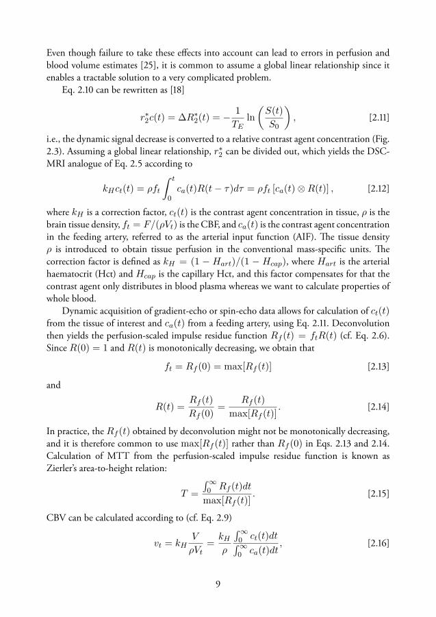
Even though failure to take these effects into account can lead to errors in perfusion andblood volume estimates [], it is common to assume a global linear relationship since itenables a tractable solution to a very complicated problem.

Eq. . can be rewritten as []

r∗2c(t) = ∆R∗2(t) = − 1

TEln

(S(t)

S0

), [.]

i.e., the dynamic signal decrease is converted to a relative contrast agent concentration (Fig..). Assuming a global linear relationship, r∗2 can be divided out, which yields the DSC-MRI analogue of Eq. . according to

kHct(t) = ρft

ˆ t

0ca(t)R(t− τ)dτ = ρft [ca(t)⊗R(t)] , [.]

where kH is a correction factor, ct(t) is the contrast agent concentration in tissue, ρ is thebrain tissue density, ft = F/(ρVt) is the CBF, and ca(t) is the contrast agent concentrationin the feeding artery, referred to as the arterial input function (AIF). e tissue densityρ is introduced to obtain tissue perfusion in the conventional mass-specific units. ecorrection factor is defined as kH = (1 − Hart)/(1 − Hcap), where Hart is the arterialhaematocrit (Hct) and Hcap is the capillary Hct, and this factor compensates for that thecontrast agent only distributes in blood plasma whereas we want to calculate properties ofwhole blood.

Dynamic acquisition of gradient-echo or spin-echo data allows for calculation of ct(t)from the tissue of interest and ca(t) from a feeding artery, using Eq. .. Deconvolutionthen yields the perfusion-scaled impulse residue function Rf (t) = ftR(t) (cf. Eq. .).Since R(0) = 1 and R(t) is monotonically decreasing, we obtain that

ft = Rf (0) = max[Rf (t)] [.]

and

R(t) =Rf (t)

Rf (0)=

Rf (t)

max[Rf (t)]. [.]

In practice, the Rf (t) obtained by deconvolution might not be monotonically decreasing,and it is therefore common to use max[Rf (t)] rather than Rf (0) in Eqs. . and ..Calculation of MTT from the perfusion-scaled impulse residue function is known asZierler’s area-to-height relation:

T =

´∞0 Rf (t)dt

max[Rf (t)]. [.]

CBV can be calculated according to (cf. Eq. .)

vt = kHV

ρVt=

kHρ

´∞0 ct(t)dt´∞0 ca(t)dt

, [.]

where the correction for Hct converts from distribution (plasma) volume fraction to wholeblood volume fraction.

Finally, it should be remembered that if two out of the three parameters (ft, vt and T )are available, the third can be calculated using the central volume theorem, vt = ftT (Eq..). e alternative expressions thus become

ft =kH´∞0 ct(t)dt max[Rf (t)]

ρ´∞0 ca(t)dt

´∞0 Rf (t)dt

, [.]

vt =

ˆ ∞

0Rf (t)dt, [.]

and

T =kH´∞0 ct(t)dt

ρ´∞0 ca(t)dt max[Rf (t)]

. [.]

Arterial input function

Many of the challenges in DSC-MRI are related to the AIF, as comprehensively reviewed byCalamante []. As mentioned previously, the relation between relaxation rate and contrastagent concentration is different for the AIFs and the tissue curves, and this is important totake into account if absolute values are warranted [, , ]. Another source of erroneousAIF registration is PVEs, and several ways to correct the AIF area have been proposed [].For example, in Paper , we used the prebolus approach in which the AIF is rescaledto the area of a venous output function (VOF) acquired from a preceding single-sliceprebolus experiment []. Another approach towards quantification in absolute terms is touse independent calibration measurements, for example, nuclear medicine based perfusionor alternative MRI measurements of CBF or CBV [, , ].

Delay and dispersion

Delay between the registered AIF and tissue curves, as well as bolus dispersion during thecorresponding transit, may lead to severe CBF quantification errors []. e most commonways to account for delay is to use a delay-insensitive deconvolution algorithm, to accountfor delay in the model, or to employ local AIFs [, , ]. Bolus dispersion refers to thecontinuous dilution of the tracer during the transit from the site of the measured AIF tothe site of the measured tissue curve, and this is a more delicate and difficult problem. Itmanifests itself as a broadening of the bolus, and is caused by the variation in blood velocityand the different pathways of the arterial system. A common way to model dispersion istherefore to use a vascular transport function ha(t) which, similarly to the capillary transittime probability distribution h(t), is the probability distribution of transit times from the

site of the measured AIF to the tissue of interest. With this definition, if c∗ais the measuredAIF, the true AIF is given by ca(t) = c∗a(t)⊗ ha(t), and Eq. can be modified to includedispersion according to

ct(t) = ft [ca(t)⊗R(t)] = ft [c∗a(t)⊗ ha(t)⊗R(t)] = ft [c

∗a(t)⊗R∗(t)] [.]

where R∗(t) = ha(t) ⊗ R(t) is the ’dispersed’ effective residue function obtained bydeconvolution if dispersion is not accounted for. Example of a vascular transport function,and the effect on the AIF and the perfusion-scaled residue function, is shown in Figure ..It can be seen that arterial dispersion leads to a distorted and non-physiological residuefunction, with corresponding underestimation of CBF (Eq. .) and overestimation ofMTT (Eq. .). ese types of distortions are the reason why perfusion is usually estimatedfrom max[Rf (t)] rather than Rf (0).

From Eq. . it is apparent that it is very difficult to separate the effects of arterialbolus dispersion and the microvascular distribution of the bolus given by the true residuefunction. To improve quantification in the presence of delay and dispersion, Willats etal. proposed the use of deconvolution methods able to recover a wider array of effectiveresidue function shapes [, ]. However, this does not correct for dispersion, and othershave attempted to model and estimate the amount of dispersion to correct for the effect[–]. Several models for ha have been suggested in the DSC-MRI and ASL literature,such as exponential [], Gaussian [, ] and gamma [, ].

As described later, both delay and dispersion were accounted for in Paper . Inparticular, delay effects were minimized by shifting signal curves prior to deconvolution,and dispersion was modeled in the form of an exponential function.

Deconvolution

Since deconvolution is a difficult operation prone to errors, some researchers have promotedthe use of qualitative (descriptive or summary) parameters. However, it has been shown thatdeconvolution is required for reliable perfusion estimation [, ]. Many deconvolutionmethods have been proposed in the literature and a brief overview is given here (see also,for example, Refs. [, ]). Deconvolution methods can be divided into two groups; modeldependent (parametric) and model independent (nonparametric or model-free) methods.

Assuming that the contrast agent’s capillary transport can be described by an analyticalfunction, the deconvolution can be realized by nonlinear least squares fitting. e mostsimple parametrization is based on the assumption of a vascular system corresponding to asingle well-mixed compartment, resulting in a mono-exponential residue function modelaccording to R(t) = e−t/T . Another approach is to model the transit time distribution, forexample using a gamma distribution []. Model-dependent deconvolution is uncommonin DSC-MRI, primarily since it only yields reliable results if the true residue function iswell-described by the model [].

0 10 20 30 40 50

0

2

4

6

8

10

c∗a(t)

t0 5 10 15 20

0

0.2

0.4

0.6

0.8

1

ha(t)

t

⊗ =

0 10 20 30 40 50

0

2

4

6

8

10

ca(t)

t

0 5 10 15 20

0

10

20

30

40

50

60

ft · R(t)

t0 5 10 15 20

0

0.2

0.4

0.6

0.8

1

ha(t)

t

⊗ =

0 5 10 15 20

0

10

20

30

40

50

60

ft · R∗(t)

t

Figure 2.4: Simulated effect of dispersion on the AIF and the estimated residue function (Eq. 2.20). The top row shows theundispersed input, the vascular transport function (gamma kernel [41]), and the resulting dispersed input function.The bottom row shows the true perfusion-scaled residue function, the vascular transport function, and the dispersedresidue function.

Model-free deconvolution methods can return residue functions that do not correspondto a particular functional shape. e main issue with model-free deconvolution is that it isan inverse problem, which tends to be ill-posed (no unique well-defined solution exists) andill-conditioned (small errors in the data are amplified in the solution), and many methodsare defined by the way in which they handle this issue. Transform methods are based onthe convolution theorem, most commonly for the Fourier transform [, , ]. esemethods are very sensitive to noise, which is usually controlled for by applying a low-passfilter that reduces high-frequency noise in the solution. Another approach for model-freedeconvolution is to employ a discrete reformulation of Eq. . according to []

kHct(tj) = ρft

ˆ tj

0ca(t)R(t− τ)d ≈ ρft∆t

j∑i=0

ca(ti)R(tj − ti), [.]

where ∆t is the temporal resolution and j denotes the time-point index. By writing Eq.. in short hand ct = caR (the constants are included in the matrices), deconvolutionmay be performed by minimizing ∥caR− ct∥22. As for the transform methods, thisapproach is very sensitive to noise, which can be controlled by minimizing the regularizedproblem ∥caR− ct∥22 + γ ∥LR∥22, where γ is the regularization parameter and L isthe regularization operator. e regularization operator is usually chosen to constrain theresolved residue function to be a nonnegative, monotonically decreasing and/or smoothfunction of time [, ].

Another common way to solve Eq. . is singular value decomposition (SVD) [].

In SVD, ca is decomposed into two orthogonal matrices and a nonnegative diagonalmatrix, and ca

−1 is expressed as a matrix product and used to estimate R. A thresholdon the diagonal matrix is used to truncate values so that non-physiological oscillations aresuppressed in the solution (regularization). e most common deconvolution method inDSC-MRI is block-circulant SVD (cSVD), which was proposed by Wu et al. to reduce thesensitivity of SVD to delay []. In the same work, an adaptive thresholding approach wasalso proposed, called oscillation-indexed block-circulant SVD (oSVD). e SVD-basedmethods are characterized by low noise sensitivity and robust results, although the resolvedresidue functions are not necessarily nonnegative or monotonically decreasing, and mayresult in perfusion underestimation. Both cSVD and oSVD were used as reference methodsin Paper .

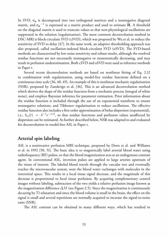
Several recent deconvolution methods are based on nonlinear fitting of Eq. .in combination with regularization, using model-free residue functions defined on acontinuous time scale [, , ]. An example of this is nonlinear stochastic regularization(NSR), proposed by Zanderigo et al. []. is is an advanced deconvolution methodwhich derives the shape of the residue function from a stochastic process (integral of whitenoise), and employs Bayesian inference for parameter estimation. Prior information aboutthe residue function is included through the use of an exponential transform to ensurenonnegative solutions, and Tikhonov regularization to reduce oscillations. e effectiveresidue function also includes a first order approximation of bolus dispersion (exponential),i.e., ha(t) = δ−1e−t/δ, so that residue functions and perfusion values unaffected bydispersion can be estimated. As further described below, NSR was adapted to and evaluatedfor deconvolution in model-free ASL in Paper .

Arterial spin labelingASL is a noninvasive perfusion MRI technique, proposed by Detre et al. and Williamset al. in [, ]. e basic idea is to magnetically label arterial blood water usingradiofrequency (RF) pulses, so that the blood magnetization acts as an endogenous contrastagent. In conventional ASL, inversion pulses are applied to large arteries upstream ofthe tissue of interest. e labeled blood travels through the vascular tree and eventuallyreaches the microvascular system, were the blood water exchanges with molecules in theinterstitial space. is results in a local tissue signal decrease, and the magnitude of thisdecrease is proportional to local tissue perfusion. By acquiring complementary controlimages without labeling, subtraction of the two yields a relative perfusion image known asthe magnetization difference ∆M (see Figure .). Since the magnetization is continuouslydecaying by T relaxation and since the blood volume is small in the brain, the effect on thesignal is small and several repetitions are normally acquired to increase the signal-to-noiseratio (SNR).

e ASL contrast can be obtained in many different ways, which has resulted in

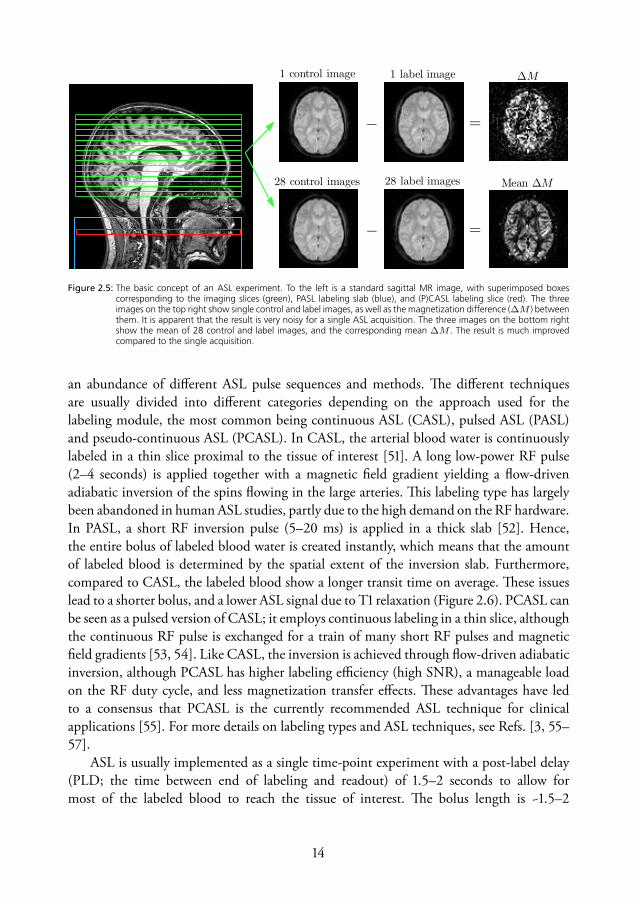
28 control images

1 control image 1 label image ∆M

− =

28 label images Mean ∆M

− =

Figure 2.5: The basic concept of an ASL experiment. To the left is a standard sagittal MR image, with superimposed boxescorresponding to the imaging slices (green), PASL labeling slab (blue), and (P)CASL labeling slice (red). The threeimages on the top right show single control and label images, as well as the magnetization difference (∆M ) betweenthem. It is apparent that the result is very noisy for a single ASL acquisition. The three images on the bottom rightshow the mean of 28 control and label images, and the corresponding mean ∆M . The result is much improvedcompared to the single acquisition.

an abundance of different ASL pulse sequences and methods. e different techniquesare usually divided into different categories depending on the approach used for thelabeling module, the most common being continuous ASL (CASL), pulsed ASL (PASL)and pseudo-continuous ASL (PCASL). In CASL, the arterial blood water is continuouslylabeled in a thin slice proximal to the tissue of interest []. A long low-power RF pulse(– seconds) is applied together with a magnetic field gradient yielding a flow-drivenadiabatic inversion of the spins flowing in the large arteries. is labeling type has largelybeen abandoned in human ASL studies, partly due to the high demand on the RF hardware.In PASL, a short RF inversion pulse (– ms) is applied in a thick slab []. Hence,the entire bolus of labeled blood water is created instantly, which means that the amountof labeled blood is determined by the spatial extent of the inversion slab. Furthermore,compared to CASL, the labeled blood show a longer transit time on average. ese issueslead to a shorter bolus, and a lower ASL signal due to T relaxation (Figure .). PCASL canbe seen as a pulsed version of CASL; it employs continuous labeling in a thin slice, althoughthe continuous RF pulse is exchanged for a train of many short RF pulses and magneticfield gradients [, ]. Like CASL, the inversion is achieved through flow-driven adiabaticinversion, although PCASL has higher labeling efficiency (high SNR), a manageable loadon the RF duty cycle, and less magnetization transfer effects. ese advantages have ledto a consensus that PCASL is the currently recommended ASL technique for clinicalapplications []. For more details on labeling types and ASL techniques, see Refs. [, –].

ASL is usually implemented as a single time-point experiment with a post-label delay(PLD; the time between end of labeling and readout) of .– seconds to allow formost of the labeled blood to reach the tissue of interest. e bolus length is ~.–

0 1 2 3 4 5 6

0

0.2

0.4

0.6

0.8

1

ca(t)

t

2αM0a ft ·

(P)CASLPASL

0 1 2 3 4 5 6

0

0.2

0.4

0.6

0.8

1

r(t)m(t)

t

⊗

0 1 2 3 4 5 6

0

2

4

6

8

10

12

∆M(t)

t

=

(P)CASLPASL

Figure 2.6: Simulation of the tracer kinetics in (P)CASL and PASL experiments using the standard model (Eq. 2.23). The leftgraph shows the input functions where (P)CASL yields a box-car bolus shape, whereas PASL yields a shorter bolusthat decreases with the T1 of blood. The middle graph shows the combined effects of the residue function andmagnetization decay by T1 relaxation. The right graph shows the resulting ASL signals. The functions start to decayafter the entire bolus has been delivered, and the stars indicate approximately when imaging is performed for asingle time point experiment.

seconds for PCASL and ~.– seconds for PASL. e experiment is repeated, usuallyuntil – control-label pairs have been acquired. Tissue signal suppression and crushingof macrovascular signal can be used to improve the quality of the perfusion images, anda reference PD image is usually acquired for calibration (i.e., determination of M0a asdescribed below). For multiple time-point (multi-TI) acquisitions, the post-label delay isusually varied between and seconds.

e general kinetic model

As mentioned in the ’Tracer kinetic modeling’ section, steady-state like experiments havebeen used in perfusion MRI, and the original ASL implementation is an example of this.Continuous labeling was applied until steady-state was reached in the tissue of interest,and subsequent perfusion estimation was achieved using the Bloch equations modified toinclude the effect of the labeled blood water [, ]. In this context, perfusion contrastwas identified as a change in the apparent T of tissue. Later on, it became more commonto use a delay between labeling and imaging, and the PASL techniques also became morecommon. erefore, the ASL analysis shifted towards a more bolus experiment orientedapproach. Buxton et al. generalized this by describing ASL from the perspective of tracerkinetic modeling, which is summarized in the so-called general kinetic model for ASL []:

∆M(t) = 2αM0a ft

ˆ t

0ca(t)r(t− τ)m(t− τ)dτ

= 2αM0a ft {ca(t)⊗ [r(t)m(t)]} . [.]

Here, ∆M(t) is the perfusion weighted tissue signal, r(t) is the residue function, m(t) isthe magnetization relaxation of the labeled water, and 2αM0aca(t) constitutes the inputfunction of labeled water, where α is the inversion efficiency, M0a is the equilibriummagnetization of arterial blood, and ca(t) is the fractional AIF. Note the analogy withthe tissue signal model in general tracer kinetics (Eq. .) and DSC-MRI (Eq. .). e

advantage of this general description is that it can be used to derive signal equations formany different labeling techniques and exchange models. Figure . displays a noise-freesimulation of the tracer kinetics in (P)CASL and PASL experiments.

e standard model

e standard model is a simplified ASL model, based on a set of assumptions, leading totractable ASL signal equations []. In short, it is assumed that labeled blood arrives at thevoxel after a delay time ∆t (arrival time), that the water exchange between blood and tissueis described by a well-mixed single-compartment, and that the labeled water upon arrivalto the voxel starts to decay with the T of tissue (T1t) rather than the T of arterial blood(T1a). ese assumptions can be formulated in terms of the time-dependent functions inEq. . according to

ca(t) = 0 t < ∆t

e−∆t/T1a ∆t < t < ∆t+ τ [(P )CASL]

e−t/T1a ∆t < t < ∆t+ τ [PASL]0 t > ∆t+ τ

r(t) = e−ftt/λ

m(t) = e−t/T1t , [.]

where τ is the label duration³ (length of the bolus) and λ is the brain-blood partitioncoefficient of water. Figure . displays these functions, together with the resulting ASLsignal (Eq. .). By inserting these expressions into the general kinetic model (Eq. .),we obtain analytical signal equations that can be applied to single- or multi-TI ASL data.In single time-point analysis, perfusion is usually estimated by directly solving the equationfor f , whereas in multi-TI analysis, the signal equation is fitted to the measured ∆M(t)curve.

By assuming that the entire bolus has been delivered to the tissue (t − τ > ∆t), thatthere is no outflow, and that the label only decays with T1a, a very basic model for singletime-point ASL is obtained according to []

∆M = 2αM0aT1aft e−w/T1a(1− e−τ/T1a) [(P )CASL]

∆M = 2αM0aτft e−TI/T1a [PASL] [.]

where w = t − τ is the PLD in (P)CASL, and TI = t is the inversion time (i.e., thetime between labeling and readout) in PASL. Note that many different assumptions arerequired to arrive at these simple and convenient signal equations, which naturally makesthem prone to errors.

³e label duration is often denoted TI1 in PASL experiments.

0 1 2 3 4-10

0

10

20

30

40

50

60

70

80

a)

Time [s]

f R

(t)

[ml/1

00g

/min

]

Residue function

cSVDoSVDNSRNSRcd

0 1 2 3 4-0.5

0

0.5

1

1.5

2

2.5

3x 10

4b)

Time [s]

M(t

) [a

.u.]

Tissue response

cSVDoSVDNSRNSRcdMeasured

Figure 2.7: Example of deconvolution results in a single voxel, from Paper . (a) NSR yields more reasonable residue functionshapes compared to SVD, especially when correcting for dispersion (NSRcd). Heavy truncation, as for oSVD in thiscase, may cause severe perfusion underestimation. (b) Measured and fitted tissue signals, ∆M(t), for the differentdeconvolution methods. The unphysiological solutions of the SVD-based deconvolution methods are the results ofoverfitting, whereas NSR trades larger residuals for smoother solutions.

Model-free arterial spin labeling

Whereas Eq. . represents one of the most simplified ways to quantify perfusion withASL, model-free ASL, devised by Petersen et al. [], is at the other end of that spectrum.It attempts to relax and reduce the number of assumptions by employing a more advancedpulse sequence that acquires additional data, allowing for quantification by means of model-free deconvolution [].e sequence is called QUASAR, and is designed to dynamicallyacquire both arterial input curves ca(t) and tissue curves ∆M(t). Similar to DSC-MRI,deconvolution of Eq. . yields the perfusion-scaled effective residue function Rf (t) =ftR(t) = ftr(t)m(t), from which a model-free perfusion estimate is obtained. ereproducibility of model-free ASL was tested in a large test-retest study including sitesand healthy subjects, using automatic planning to yield consistent slice positioning[]. In an alternative approach, Chappell et al. suggested a model-based analysis ofQUASAR data, including modeling of arterial dispersion []. e results of that studyindicated the presence of substantial dispersion effects in QUASAR data.

e QUASAR sequence employs pulsed labeling and saturation recovery (SR) Look-Locker readout. e application of arterial crushers allows for estimation of ca(t) curves bysubtraction of∆M(t)with and without crushers. By identifying local AIFs with reasonableshape and SNR, voxel-wise AIFs can be calculated by appropriate scaling []. e SRsignal evolution of the control images allows for mapping of M0a and T1t, which are usedin the quantification. Furthermore, in Paper , we exploited the SR data to obtain PVestimates, subsequently used to produce tissue region of interests (ROIs) and improve theM0a estimation.

Due to the similarity with model-free quantification in DSC-MRI, results from model-free ASL are expected to be dependent on the applied deconvolution method, and be

sensitive to delay and dispersion. erefore, in Paper , we assessed the dependence ofmodel-free ASL on the choice of deconvolution method, and the possibility to correctfor delay and dispersion. Specifically, SVD-based deconvolution was used in the originalmodel-free ASL work [], whereas we adapted the NSR deconvolution method (describedabove) []. Even with truncation, the SVD-based deconvolution methods generatessolutions with unphysiological oscillations and negative values, and the NSR deconvolutionwas shown to improve this also for model-free ASL. Figure . displays residue functionsand signal fits for the NSR and SVD deconvolution methods. NSR with dispersioncorrection (NSRcd) clearly results in more physiologically plausible residue functions, i.e.,monotonically decreasing nonnegative solutions.

A central motivation for this work was that truncated SVD generates can lead toperfusion underestimation [], whereas NSR has been shown to better resolve theperfusion-scaled residue function in DSC-MRI []. is was verified in Paper usingsimulations, and the more advanced NSR deconvolution method also yielded in vivo resultsin better agreement with literature perfusion values. NSR is delay sensitive, which wasaccounted for by employing edge detection and temporal shifting of the concentrationcurves prior to deconvolution. Finally, NSR includes simple dispersion modelling, andinitial results suggested that NSR deconvolution can potentially correct for dispersioneffects in model-free ASL. Figure . shows examples of the in vivo results from Paper, including dependence on the applied deconvolution method, the relation betweendispersion and arrival time, and PV maps. Model-free ASL was also used in Paper , whichwill be further discussed in Chapter .

pCSF

i)

[%]0

20

40

60

80

100

pWM

h)

[%]0

20

40

60

80

100

pGM

g)

[%]0

20

40

60

80

100

0 0.5 1 1.5 20

0.05

0.1

0.15

r = 0.93

∆ t vs δ

∆ t

δ

f)

δe)

[s]0

0.05

0.1

0.15

∆ td)

[s]0

0.5

1

1.5

2

∆ fNSRcd−cSVD

c)

[ml/100g/min]−30

−20

−10

0

10

20

30

foSVD

b)

[ml/100g/min]0

10

20

30

40

50

60

fNSRcd

a)

[ml/100g/min]0

10

20

30

40

50

60

Figure 2.8: Example of group averaged (10 subjects) parameter maps in MNI space, from the model-free ASL results in Paper .The top row shows CBF obtained with (a) NSR deconvoution, (b) SVD deconvolution and (c) the difference betweenthe two. There is a considerable difference and, in particular, higher gray matter values are obtained with NSR. Thesecond row shows (d) the arrival time ∆t, (e) the amount of dispersion δ, and (f) the correlation between theseparameters. The high correlation suggests that the dispersion modeling worked as intended, since more dispersionis expected for blood that has traveled longer. The bottom row displays PV maps for (g) gray matter, (h) white matter,and (i) cerebrospinal fluid, obtained using the SR data (see Chapter 3).

Chapter

Partial volume mapping

e partial volume effect (PVE) in MRI refers to the intravoxel mixing of signals fromdifferent components that occurs due to the limited spatial resolution []. PVE-basedsegmentation, or PV mapping, is a type of image segmentation in which this effect is takeninto account, so that the amount of each tissue type is estimated in every voxel []. SincePV mapping estimates tissue volume at a sub-voxel level, it is more versatile than hardbinary segmentation and can be used to improve volume metrics and quantitative MRI.For example, a PV mapping method referred to as ’fractional signal modeling’ (FSM) wasused in Paper for improved M0a estimation, as well as in Papers – for PVC of ASLand DSC-MRI data. Furthermore, a new FSM method was proposed in Paper . FSM isbased on quantitative relaxometry, as will be described later in this chapter.

SegmentationImage segmentation is the process of dividing an image into different segments (andsometimes to classify those segments) based on features such as intensity, pattern or otherproperties. Segmentation is a very broad issue which has attracted a lot of attention indigital image processing, including medical imaging and in particular MRI [, ]. Adetailed discussion about methods and applications is outside the scope of this thesis, andwe will only briefly discuss human brain segmentation. Brain segmentation often refers toautomatic segmentation of a brain image into three different tissue types, i.e., gray matter(GM), white matter (WM), and cerebrospinal fluid (CSF), although the concept mayalso include other processes such as brain extraction (skull stripping) and segmentation oflesions/pathologies []. Many different segmentation methods exist, and the more robustmethods are often advanced and may be difficult to implement. Fortunately, easy-to-usetools are freely available as part of standard software packages for brain image processing.

Generally speaking, segmentation is a difficult problem due to measurement noise,image artifacts, bias fields, complex anatomical structures and limited spatial resolution.

On the other hand, MRI has excellent soft tissue contrast and the main intracranial tissuetypes are few and generally form continuous shapes, which makes brain segmentationfeasible with some work. Although this chapter is focused on automatic segmentation, it isimportant to note that manual delineation of ROIs is very common in clinical routine.

Most brain segmentation methods are based on the use of image intensity orquantified tissue properties. is is intuitively reasonable because many MRI sequencesyield signal intensities that differ between GM, WM and CSF. e simplest intensity-basedsegmentation is to threshold the image, so that all voxels within a certain intensity rangeare assigned to a certain tissue type, but this approach generally leads to poor segmentationresults. Inclusion of several different images is likely to improve the results (i.e., multi-spectral segmentation), for example, using multi-contrast or quantitative images togetherwith predefined regions in feature space [–]. e advantage of using quantitativeimages is that the algorithm do not have to account for arbitrary and biased signal values(which can depend on hardware and protocol). Since the segmentation methods rely ontissue-specific signals, the characteristics needs to be pre-defined or estimated from theimage (feature extraction).

A more advanced approach is to model the signal from each tissue type with aprobability distribution (e.g., Gaussian mixture models), and to include regularization byspatial prior information to make the segmentation less noise sensitive. us, each voxel isassigned a probability of belonging to a certain class, based on the relative contribution ofthe distribution at the given intensity value, accounting for the prior information. Notethat these probability values are continuous on the scale –, and relate to the PVE-based segmentation methods discussed below. A traditional prior is to assume that mostvoxels are surrounded by voxels of the same class, which can be incorporated using Markovrandom field theory []. Another common regularization technique is to use registrationto a stereotactic standard brain (spatial normalization), and subsequent segmentationusing population-based priors/atlases []. is technique is employed within a statisticalframework in the segmentation tool included in the SPM software package [], whichwas used in the reference method in Paper . Population-based atlases also allow for furtherparcellation of structures (i.e., to label subregions within the different tissue types, such ascortical regions and deep gray matter structures).

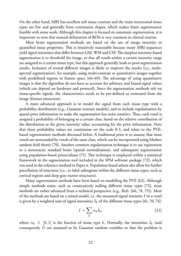
Many segmentation methods have been based on modelling the PVE []. Althoughsimple methods exists, such as consecutively nulling different tissue types [], mostmethods are rather advanced from a technical perspective (e.g., Refs. [, , ]). Mostof the methods are based on a mixed model, i.e. the measured signal intensity I in a voxelis given by a weighted sum of signal intensities Ik of the different tissue types [, , ]:

I =∑k

αkIk, [.]

where αk ∈ [0, 1] is the fraction of tissue type k. Normally, the intensities Ik (andconsequently I) are assumed to be Gaussian random variables so that the problem is

Threshold

CS

F

SPM FSM (IR) FSM (VFA)

GM

WM

Figure 3.1: Side by side comparison of segmentation and PV mapping using, from left to right, simple thresholding, the SPMsoftware, IR-based FSM and VFA-based FSM. The FSM methods produce more nuanced images including mixture oftissue types, whereas thresholding and the SPM software results in more traditional and binary segmentation.

tractable with statistical approaches []. e FSM methods discussed later can be seenas an extension of the model in Eq. ., but with the individual Ik being functions ofacquisition and tissue parameters, modelled according to MR signal equations.

Intensity-based segmentation is difficult, not only due to signal overlap and mixedvoxels, but also due to noise and bias fields. erefore, denoising and bias field correction isnormally included in the preprocessing. In summary, most current segmentation algorithmsoperate in a few well-defined steps, namely pre-processing (e.g., denoising, inhomogeneitycorrection and skull-stripping), feature extraction, and segmentation/classification. Manymore and advanced segmentation methods exist that are not discussed here, e.g. fuzzy logics,Bayesian inference and Markov random fields [, ].

Traditional applications of brain segmentation includes identification of ROIs fordiagnosis or treatment/surgical planning, preprocessing for subsequent image processing,abnormality detection, and for regional analysis of MRI data []. More recentapplications based on PV mapping include volumetry [], diagnosis and prognosis ofneurodegenerative diseases [], and improvements in quantitative MRI (see Chapter ).e FSM implementation described in Paper could be used in any type of application,whereas examples of FSM applications can be found in Papers –.

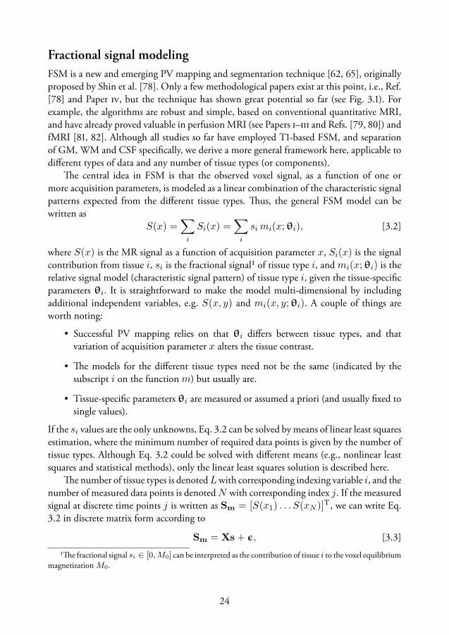
Fractional signal modelingFSM is a new and emerging PV mapping and segmentation technique [, ], originallyproposed by Shin et al. []. Only a few methodological papers exist at this point, i.e., Ref.[] and Paper , but the technique has shown great potential so far (see Fig. .). Forexample, the algorithms are robust and simple, based on conventional quantitative MRI,and have already proved valuable in perfusion MRI (see Papers – and Refs. [, ]) andfMRI [, ]. Although all studies so far have employed T-based FSM, and separationof GM, WM and CSF specifically, we derive a more general framework here, applicable todifferent types of data and any number of tissue types (or components).

e central idea in FSM is that the observed voxel signal, as a function of one ormore acquisition parameters, is modeled as a linear combination of the characteristic signalpatterns expected from the different tissue types. us, the general FSM model can bewritten as

S(x) =∑i

Si(x) =∑i

simi(x;θi), [.]

where S(x) is the MR signal as a function of acquisition parameter x, Si(x) is the signalcontribution from tissue i, si is the fractional signal¹ of tissue type i, and mi(x;θi) is therelative signal model (characteristic signal pattern) of tissue type i, given the tissue-specificparameters θi. It is straightforward to make the model multi-dimensional by includingadditional independent variables, e.g. S(x, y) and mi(x, y;θi). A couple of things areworth noting:

• Successful PV mapping relies on that θi differs between tissue types, and thatvariation of acquisition parameter x alters the tissue contrast.

• e models for the different tissue types need not be the same (indicated by thesubscript i on the function m) but usually are.

• Tissue-specific parameters θi are measured or assumed a priori (and usually fixed tosingle values).

If the si values are the only unknowns, Eq. . can be solved by means of linear least squaresestimation, where the minimum number of required data points is given by the number oftissue types. Although Eq. . could be solved with different means (e.g., nonlinear leastsquares and statistical methods), only the linear least squares solution is described here.

e number of tissue types is denotedLwith corresponding indexing variable i, and thenumber of measured data points is denoted N with corresponding index j. If the measuredsignal at discrete time points j is written as Sm = [S(x1) . . . S(xN )]T, we can write Eq.. in discrete matrix form according to

Sm = Xs+ ϵ, [.]

¹e fractional signal si ∈ [0,M0] can be interpreted as the contribution of tissue i to the voxel equilibriummagnetization M0.

where Xji = mi(xj ;θi), s = [s1 . . . sL]T and ϵ is a N × 1 noise vector. Now, Eq. .

can be solved for s with linear least squares estimation. Since si values are nonnegativeand sum up to M0, the estimation can benefit from using constrained least squares, i.e.,minimization of ∥Xs− Sm∥22 subject to s ≥ 0 and/or

∑i si = M0.

PV estimates in units of relative voxel volume, pi ∈ [0, 1], can be obtained fromthe fractional signal estimates by accounting for tissue-specific water densities ρi andnormalizing:

pi =si/ρi∑i si/ρi

. [.]

An interesting feature of FSM is that, as long as unique characteristic tissue signals canbe reasonably established, the PV estimates do not depend on quantitative values for θi,and they are insensitive to spatially varying scaling factors such as B−. However, any spatialvariation of the true characteristic curves (e.g., due to spatial variations in θi or B+) willlead to errors unless accounted for. is leads us to one of the most crucial parts of FSM,namely how to determine the θi values.

For T-based FSM, a few different ways to set the tissue specific T values (T1i) havebeen suggested. e most simple approach is to use fixed literature values []. However, thisapproach is highly sensitive to inter-subject variations and, therefore, Shin et al. suggestedto estimate T1i values subject-wise by employing standard T mapping and subsequentanalysis of the whole-brain histogram, as a pre-processing step (see Figure . and Ref.[]). However, due to the small CSF volume, literature values are often used for CSF(one exception being Paper in which CSF T was estimated from a ventricle region).In a low-resolution application, Petr et al. argued that the resolution was too low to allowfor estimation of GM T from the histogram analysis, and instead adopted a least squaresiterative estimation []. Even ifT1i values are estimated on a subject basis, the within-tissueT1i values are fixed, which corresponds to an assumption that representative values existsfor each tissue type. To relax this assumption, Oliver suggested to let GM T vary spatially(regularizing the problem by constraining the value to be fixed in a local region), whichimproved classification of deep GM structures []. Further investigation and developmentof the handling of θi in FSM analysis is needed, which could include assessment of spatialpriors and statistical approaches.

We want to stress the impressive robustness, in relation to its simplicity, that FSMexhibits. While most segmentation methods discussed above require many differentprocessing steps, and are very complex and difficult to implement (which leads to higherdemand on expertise and less accessible code []), the FSM technique is, in its basic form,very simple. For example, FSM can be implemented with just one extra processing stepadded to a standard T quantification script. Although multiple acquisitions are required,the data can be acquired with conventional and widely available pulse sequences. Anotheradvantage is that FSM is, to a large extent, independent on hardware and protocol settingsand does not rely on predefined tissue maps or features, which makes it applicable to awider range of individuals such as different ages and patient groups [].

Inversion and saturation recovery acquisition

e most common method to date has been T-based FSM, in particular using inversionrecovery (IR) and SR data. Assuming that the repetition time TR ≫ T1 and disregardingT-weighting, the signal equation for a standard IR or SR sequence is given by S(t) =M0(1 − Ae−t/T1), where M0 is the equilibrium magnetization, and A = (1 − cos θ),where θ is the flip angle of the preparation pulse. us, A = 2 for an ideal inversionand A = 1 for an ideal saturation, and t is usually denoted TI and TS for IR and SR,respectively. By using the standard signal equation as a basis for mi(x;θi), the IR/SR-based FSM model becomes

S(t) =∑i

sim(t;T1i) =∑i

si (1−Ae−t/T1i), [.]

where T1i is the T of tissue i. Note that M0 is included in the si values rather thanm(t;T1i). As an example of FSM analysis, a post-processing pipeline for SR-based FSMis summarized graphically in Figure .. In contrast to many signal intensity basedsegmentation algorithms, the widths of the different peaks in the histogram are not usedhere.

In the original paper, Shin et al. used a special IR sequence with Look-Locker EPIreadout in steady-state, and called that FSM implementation ’fractional signal mappingfrom inversion recovery’ (FRASIER) []. e Look-Locker readout employs a train oflow flip angles to rapidly acquire images at different times t. is results in a steady statemagnetization given by

M∗0 = M0

1− e−∆T/T1

1− cosϕ · e−∆T/T1, [.]

and a corresponding apparent longitudinal relaxation time given by1

T ∗1

=1

T1− ln(cosϕ)

∆T, [.]

where∆T is the time between successive RF pulses, and ϕ is the flip angle of those pulses. Ifthe inversion pulse is applied at steady state, and including the effects of the Look-Lockerreadout, the signal recovery follows S(t) = M∗

0 (1 − Ae−t/T ∗1 ), and the corresponding

FSM model becomes []

S(t) =∑i

si1− e−∆T/T1i

1− cosϕ · e−∆T/T1i(1−Ae−t/T ∗

1i), [.]

which can be solved by linear least squares estimation as described above.is implementation of FSM was proposed in [], and was employed in Papers –

and Refs. [–]. In Paper , simulations suggested good performance of FSM applied tonative low-resolution ASL data. It should be noted that Shin et al. assumed ideal inversionpreparation (A = 2) and excitation pulses [], whereas we accounted for non-idealsaturation preparation and spatial variation of ϕ in Papers –.

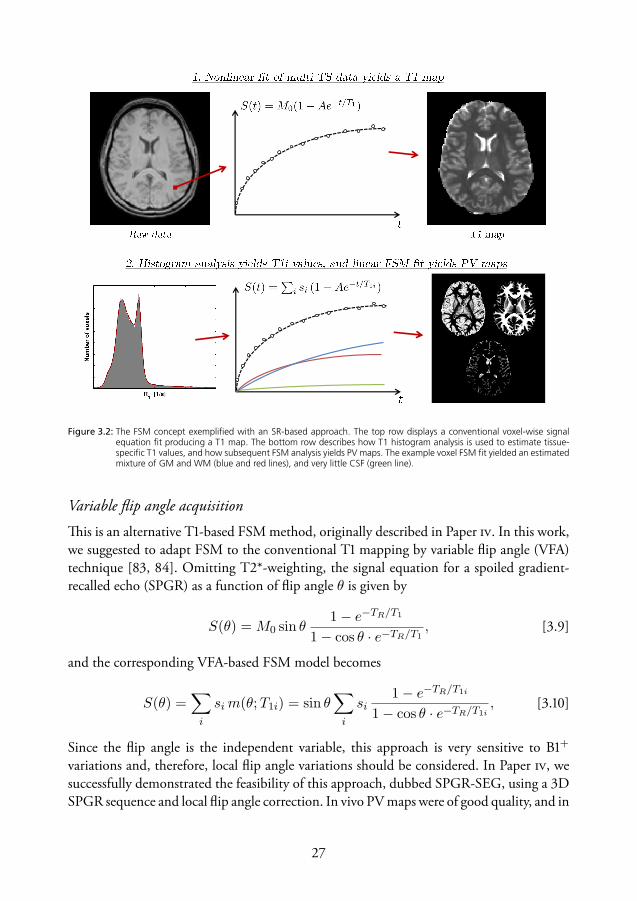
Figure 3.2: The FSM concept exemplified with an SR-based approach. The top row displays a conventional voxel-wise signalequation fit producing a T1 map. The bottom row describes how T1 histogram analysis is used to estimate tissue-specific T1 values, and how subsequent FSM analysis yields PV maps. The example voxel FSM fit yielded an estimatedmixture of GM and WM (blue and red lines), and very little CSF (green line).

Variable flip angle acquisition

is is an alternative T-based FSM method, originally described in Paper . In this work,we suggested to adapt FSM to the conventional T mapping by variable flip angle (VFA)technique [, ]. Omitting T*-weighting, the signal equation for a spoiled gradient-recalled echo (SPGR) as a function of flip angle θ is given by

S(θ) = M0 sin θ1− e−TR/T1

1− cos θ · e−TR/T1, [.]

and the corresponding VFA-based FSM model becomes

S(θ) =∑i

sim(θ;T1i) = sin θ∑i

si1− e−TR/T1i

1− cos θ · e−TR/T1i, [.]

Since the flip angle is the independent variable, this approach is very sensitive to B+

variations and, therefore, local flip angle variations should be considered. In Paper , wesuccessfully demonstrated the feasibility of this approach, dubbed SPGR-SEG, using a DSPGR sequence and local flip angle correction. In vivo PV maps were of good quality, and in

CSF GM WM

Figure 3.3: Example of T2-based FSM results achieved using T2-preparation (unpublished data). The T2 contrast between GMand WM is smaller than the corresponding T1 contrast, but T2-based FSM still seems feasible.

good agreement with IR-based FSM (Figure .). Simulations suggested good performanceat reasonable SNR levels, and indicated that separation of a fourth component (e.g., alesion) would be challenging with the current protocol.

Note that different types of linearizations of Eq. . exist, which could be used for fasterT mapping and be incorporated in the FSM model. However, such transforms leads to anon-symmetric noise distribution which makes the fitting less straight-forward.

Variable T weighting

By acquiring images with different T weightings (e.g., different echo times or T-preparation), T-based FSM can be achieved. For a standard spin or gradient multi-echoacquisition, S(TE) = M0e

−TE/T(∗)2 , and the T-based FSM model becomes

S(TE) =∑i

simi(TE ;T(∗)2i ) =

∑i

si e−TE/T

(∗)2i , [.]

In a preliminary study, low-resolution T-based FSM by variable T-preparation yieldedreasonable results (see Figure .).

Other contrasts and multi-dimensional acquisition

Any variable weighting that yields sufficient contrast between different tissue types can,in theory, be used for FSM-based PV mapping and segmentation. In addition to T-and T-weighting, magnetization transfer contrast might be a potential contender. Asfor conventional segmentation approaches, FSM is likely to benefit from employmentof a multi-spectral approach, for example, combining variable T- and T-weighting.

is could potentially enable separation of more components or improve segmentationof challenging structures such as deep GM.

Diffusion MRI has a long history of multi-component modeling approaches similar toFSM, although these have often been focused on improving diffusion metrics rather thanestimating volumes. Although CSF-to-parenchyma contrast is high in diffusion MRI, itis difficult to separate GM and WM based solely on the diffusion coefficient. However,diffusion contrast can differ between other components, and this has been exploited using,for example, bi-exponential fitting with low b-values to separate blood and tissue (seeChapter ), bi-exponential fitting using high b-values to separate fast and slow diffusioncompartments [], or fitting of multiple tensor models to separate intra-cellular, extra-cellular and free water [, ].

Chapter

Partial volume correction in perfusionMRI

e partial volume effectAs described in the previous chapter, PVEs occur due to the limited spatial resolutionrelative to the size of the features that are being imaged. Hence, the signal does not onlydepend on the experimental settings and the intrinsic properties of a given tissue, but alsoon the relative contribution of each tissue type to the mixed voxel signal []. For example,in nuclear medicine, the effective spatial resolution is determined by a combination ofthe voxel size and the point spread function []. e corresponding PVEs are known asthe sampling effect and spill-in/spill-out effects, respectively. In MRI, on the other hand,the spatial resolution is often determined exclusively by the voxel size, because the pointspread function is often smaller than the voxel size []. is means that we usually donot have to consider signal components originating from neighboring voxels influencingthe voxel of interest (one exception being readout modules that yields substantial spatialblurring). In general, functional imaging techniques tend to employ lower resolution thanmorphological imaging, leading to more severe PVEs. For example, PVEs impede theinterpretation of brain perfusion MRI, especially in thin cortical GM. Errors in tissueperfusion estimates can thus occur due to a mixture of GM and WM perfusion signals,or due to contamination with non-perfused tissue such as CSF.

Arterial spin labeling

Due to the limited SNR, ASL experiments include repeated data collection with low spatialresolution, of which the latter results in considerable PVEs (see Fig. .). e mixed ASLsignal can be modelled according to [, ]

∆M =∑i

pi∆Mi = pGM∆MGM+pWM∆MWM+pCSF∆MCSF+pa∆Ma, [.]

where pi represents the PV values and ∆Mi is the magnetization difference of tissuei (which can be modeled as a function of time for multi-TI applications []). Notethat ∆MCSF is usually set to zero, and most studies also omit the arterial blood signalcontribution (pa∆Ma), which is valid if the arterial blood signal is negligible or properlycrushed. In the original ASL PVC paper, Asllani et al. also included tissue-specificequilibrium magnetizations (M0i) in the PVE model [], whereas most subsequent studieshave settled with only estimating ∆Mi, which has the benefit of simplifying the post-processing.

e PVE for the voxel perfusion can in turn also be modeled as a weighted sumaccording to

ft =∑i

pi∆Mi

M0aGi =

∑i

pifi, [.]

where Gi includes the factors needed to convert ∆Mi/M0a to perfusion values fi (i.e., theremaining part of the ASL model, including tissue-specific and acquisition parameters).is model is convenient since it is immediately seen that if, for example, the arterial bloodis not crushed and not accounted for, tissue perfusion will be overestimated in proportionto the partial volume of arterial blood. If we set ∆MCSF and ∆Ma to zero, and assumethat GGM = GWM , a simplified PVE perfusion model is obtained according to

ft = pGMfGM + pWMfWM . [.]

is simplification was used in Papers –.

Dynamic susceptibility contrast MRI

All previous PVC studies in perfusion MRI have been focused on ASL. Although DSC-MRI generally employ higher resolution than ASL, PVEs could still be a source of error intissue-specific perfusion estimation. erefore, in Paper , we wanted to assess the PVEsand the possibility to perform PVC in DSC-MRI. e mixed DSC-MRI signal can bewritten as (cf. Eq. .)

S(t) =∑i

piSi(t) = S0

∑i

pi e−TE [R2i+∆R∗

2i(t)]

= S0

∑i

pi e−TE [R2i+r∗2ici(t)], [.]

where subscript i denotes tissue-specific quantities. is model could potentially be fittedto the data as is, although we opted for a simpler approach in the form of a post-hoc PVC,based on a simplified PVE model.

First, we assumed that r∗2 is equal in GM and WM, as predicted by simulations [].By factoring out the native relaxation rates R2i, and acknowledging that cCSF (t) = 0,

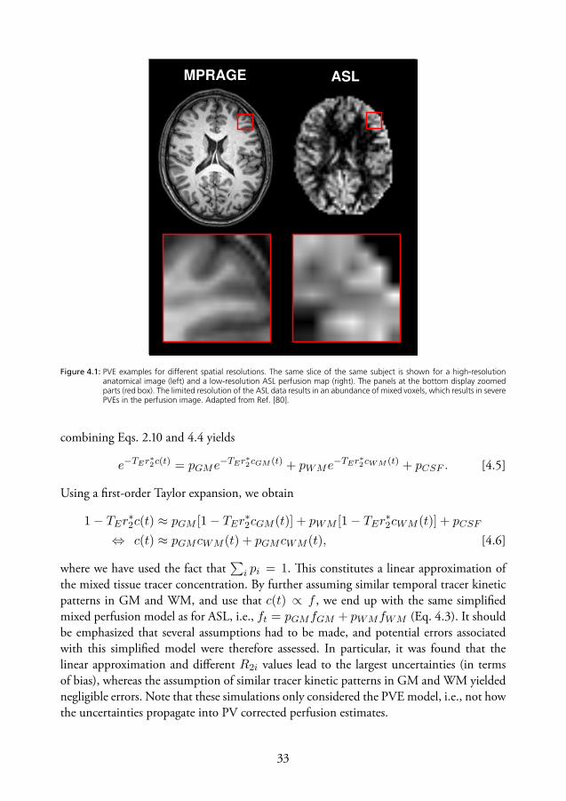
ASLMPRAGE

Figure 4.1: PVE examples for different spatial resolutions. The same slice of the same subject is shown for a high-resolutionanatomical image (left) and a low-resolution ASL perfusion map (right). The panels at the bottom display zoomedparts (red box). The limited resolution of the ASL data results in an abundance of mixed voxels, which results in severePVEs in the perfusion image. Adapted from Ref. [80].

combining Eqs. . and . yields

e−TEr∗2c(t) = pGMe−TEr∗2cGM (t) + pWMe−TEr∗2cWM (t) + pCSF . [.]

Using a first-order Taylor expansion, we obtain

1− TEr∗2c(t) ≈ pGM [1− TEr

∗2cGM (t)] + pWM [1− TEr

∗2cWM (t)] + pCSF

⇔ c(t) ≈ pGMcWM (t) + pGMcWM (t), [.]

where we have used the fact that∑

i pi = 1. is constitutes a linear approximation ofthe mixed tissue tracer concentration. By further assuming similar temporal tracer kineticpatterns in GM and WM, and use that c(t) ∝ f , we end up with the same simplifiedmixed perfusion model as for ASL, i.e., ft = pGMfGM + pWMfWM (Eq. .). It shouldbe emphasized that several assumptions had to be made, and potential errors associatedwith this simplified model were therefore assessed. In particular, it was found that thelinear approximation and different R2i values lead to the largest uncertainties (in termsof bias), whereas the assumption of similar tracer kinetic patterns in GM and WM yieldednegligible errors. Note that these simulations only considered the PVE model, i.e., not howthe uncertainties propagate into PV corrected perfusion estimates.

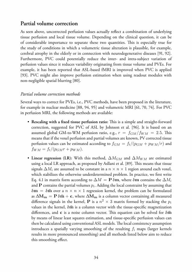
Partial volume correctionAs seen above, uncorrected perfusion values actually reflect a combination of underlyingtissue perfusion and local tissue volume. Depending on the clinical question, it can beof considerable importance to separate these two quantities. is is especially true forthe study of conditions in which a volumetric tissue alteration is plausible, for example,cerebral atrophy in the elderly or in connection with neurodegenerative diseases [, ].Furthermore, PVC could potentially reduce the inter- and intra-subject variation ofperfusion values since it reduces variability originating from tissue volume and PVEs. Forexample, it has been reported that ASL-based fMRI is improved when PVC is applied[]. PVC might also improve perfusion estimation when using readout modules withnon-negligible spatial blurring [].

Partial volume correction methods

Several ways to correct for PVEs, i.e., PVC methods, have been proposed in the literature,for example in nuclear medicine [, , ] and volumetric MRI [, , ]. For PVCin perfusion MRI, the following methods are available:

• Rescaling with a fixed tissue perfusion ratio: is is a simple and straight-forwardcorrection, suggested for PVC of ASL by Johnson et al. []. It is based on anassumed global GM-to-WM perfusion ratio, e.g., r = fGM/fWM = 2.5. ismeans that if the voxel perfusion and partial volumes are known, PV corrected tissueperfusion values can be estimated according to fGM = ft/(pGM + pWM/r) andfWM = ft/(pGMr + pWM ).

• Linear regression (LR): With this method, ∆MGM and ∆MWM are estimatedusing a local LR approach, as proposed by Asllani et al. []. is means that tissuesignals ∆Mi are assumed to be constant in a n × n × 1 region around each voxel,which stabilizes the otherwise underdetermined problem. In practice, we first writeEq. . in matrix form according to ∆M = P δm, where δm contains the ∆Mi

and P contains the partial volumes pi. Adding the local constraint by assuming thatδm = δm̄ over a n × n × 1 regression kernel, the problem can be formulatedas ∆Mm = P δm̄ + ϵ, where ∆Mm is a column vector containing all measureddifference signals in the kernel, P is a n2 × 3 matrix formed by stacking the pivalues in the kernel, δm̄ is a column vector with the tissue-specific magnetizationdifferences, and ϵ is a noise column vector. is equation can be solved for δm̄by means of linear least squares estimation, and tissue-specific perfusion values canthen be calculated using conventional ASL models. e local consistency assumptionintroduces a spatially varying smoothing of the resulting fi maps (larger kernelsresults in more pronounced smoothing) and all methods listed below aim to reducethis smoothing effect.

• Bayesian inference: is PVC approach was originally proposed by Chappell et al.for multiple time-point ASL data []. ey modeled ∆M(t) as a weighted sum ofthe individual kinetic tissue signals (including the macrovascular component), whichin turn were based on standard ASL models. e Bayesian inference was based on aMarkov random field including several parameter priors, as well as adaptive spatialpriors on fGM and fWM , meaning that the amount of smoothing is inferred fromthe data and can vary across the brain. e adaptive spatial priors were implementedspecifically to minimize the smoothing effect inherent to the LR method.

• Modified least trimmed squares (mLTS): is method, proposed by Liang et al [],is similar to LR but uses iterative ranking of residuals and matrix trimming. For ann×n kernel, an initial subset is built by successively adding ∆M values that are closeto the central kernel value, until rank is reached. Initial ∆Mi estimates are thenobtained by standard LR on that subset. Next, the residuals are calculated and sorted,and the n×n×α voxels with smallest residuals are used to form a new subset, whereα is the trimming factor. e estimation, ranking and trimming is then repeated afixed number of times, and the final ∆Mi estimates are used to calculate fi values.As with the Bayesian approach, mLTS has been shown to yield a lower degree ofsmoothing compared to LR.

• Expectation maximization and linear regression (EM-LR): Liu et al. suggested aPVC method exploiting temporal information in terms of the repeated acquisitionsin ASL []. A statistical model is used so that each single ∆M (from the repeatedacquisition) is considered to be an observation of a random Gaussian variable forwhich the mean and standard deviation are parameters to be estimated. Since thesum of two Gaussian variables is Gaussian, the problem can be solved numericallywith a conventional EM estimation. Spatial information was indirectly incorporatedby using the LR method on each measured ∆M for calculation of voxel-wise initialparameter estimates, which yielded better results and faster convergence comparedto EM with fixed initial estimates. Note that no regression kernel is used for the EMestimation.

• Weighted ridge regression (WRR): To reduce the smoothing effect of LR, a smallerkernel can be used. However, this reduces the amount of available data leading torank deficiency and high sensitivity to noise. In ridge regression, this is circumventedby introducing a bias in the estimator, i.e., trading some bias for a reduction invariance. In weighted regression, different data points are given different weights,usually to account for outliers and variable uncertainty in data. e weights can bepredetermined (e.g., a Gaussian function) or estimated from the data (e.g., robustregression). Weighted ridge regression (WRR) combines the two, and the biased andweighted estimator can be formulated as β̂WRR = (XTWX + λI)−1XTWY,where X is the design matrix, W is a diagonal matrix containing the weights, λ is

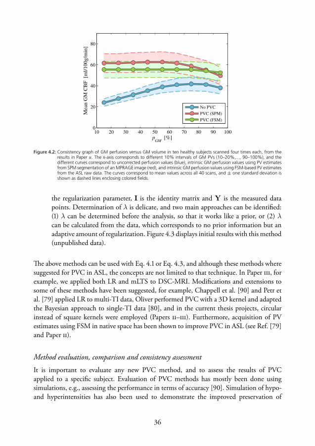
10 20 30 40 50 60 70 80 90 1000

20

40

60

80

pGM

[%]

Mea

n G

M C

BF

[m

l/100g/m

in]

No PVC

PVC (SPM)

PVC (FSM)

Figure 4.2: Consistency graph of GM perfusion versus GM volume in ten healthy subjects scanned four times each, from theresults in Paper . The x-axis corresponds to different 10% intervals of GM PVs (10–20%,..., 90–100%), and thedifferent curves correspond to uncorrected perfusion values (blue), intrinsic GM perfusion values using PV estimatesfrom SPM segmentation of an MPRAGE image (red), and intrinsic GM perfusion values using FSM-based PV estimatesfrom the ASL raw data. The curves correspond to mean values across all 40 scans, and ± one standard deviation isshown as dashed lines enclosing colored fields.

the regularization parameter, I is the identity matrix and Y is the measured datapoints. Determination of λ is delicate, and two main approaches can be identified:() λ can be determined before the analysis, so that it works like a prior, or () λcan be calculated from the data, which corresponds to no prior information but anadaptive amount of regularization. Figure . displays initial results with this method(unpublished data).

e above methods can be used with Eq. . or Eq. ., and although these methods wheresuggested for PVC in ASL, the concepts are not limited to that technique. In Paper , forexample, we applied both LR and mLTS to DSC-MRI. Modifications and extensions tosome of these methods have been suggested, for example, Chappell et al. [] and Petr etal. [] applied LR to multi-TI data, Oliver performed PVC with a D kernel and adaptedthe Bayesian approach to single-TI data [], and in the current thesis projects, circularinstead of square kernels were employed (Papers –). Furthermore, acquisition of PVestimates using FSM in native space has been shown to improve PVC in ASL (see Ref. []and Paper ).

Method evaluation, comparison and consistency assessment

It is important to evaluate any new PVC method, and to assess the results of PVCapplied to a specific subject. Evaluation of PVC methods has mostly been done usingsimulations, e.g., assessing the performance in terms of accuracy []. Simulation of hypo-and hyperintensities has also been used to demonstrate the improved preservation of

boundaries of the Bayesian, mLTS and EM-LR methods, as compared to LR [, , ].It is difficult to assess a PVC method applied to in vivo data since no ground truth is

available and, therefore, many researchers have used a reference PVC method or setting forcomparison. For example, a good kernel size or preferred PV mapping technique can beinformed by root mean square deviation of the PVC regression [, ], and the amount ofsmoothing can be compared with a reference method using an image gradient score [].Most PVC studies display the consistency of mean tissue perfusion values across differentintervals of tissue volume, as shown in Figure .. is is a compact and intuitive wayto demonstrate the dependence of the perfusion estimates on tissue volume. In Paper it was found that PV mapping based on native space ASL data improved the consistencycompared to segmentation of a high-resolution anatomical image (Fig. .), in agreementwith Ref. []. is type of plot was also used in Paper , where it was found that PVCbased on LR showed a higher consistency than mLTS. Note that, due to the smoothingeffect of some PVC methods, and since the true underlying perfusion is not necessarilyindependent on PV values, a straight line cannot unequivocally be regarded as the groundtruth.

Similar to how Shin et al. evaluated IR-based FSM [], Kuijer et al. suggested tovalidate PVC results by artificially lowering the spatial resolution through downsamplingand smoothing of both PV and perfusion data []. e idea here is that, if the PVC worksas intended, tissue-specific perfusion estimates should not be altered upon downsamplingor smoothing. e authors found that, while simulated data passed this consistency check,in vivo data did not (downsampling and smoothing increased GM perfusion estimates).Whereas the reason for this failure was unclear, it did not seem to be due to spatial mismatchor a non-ideal point spread functions, which is in agreement with another study on therobustness of PVC in ASL with respect to mismatch and resolution issues [].

Interpreting partial volume corrected perfusion

Figure . displays examples of parameter maps obtained from an ASL PVC analysis. Somevariety can be found in the reporting of PV corrected perfusion estimates, for example,tissue-specific perfusion values have been reported both in terms of partial tissue perfusionvalues pifi, and in terms of intrinsic tissue perfusion values fi. e two definitions originatefrom two different ways of acknowledging PVEs.

e former approach views PVC as a way to separate the perfusion contribution fromdifferent components. is has a strong connection to nuclear medicine where the totalnumber of counts or the total radioactivity for a specific tissue type or region is of interest.In the case of perfusion MRI, this approach can be used if estimation of the total blooddelivery to a specific tissue type is of interest. Note that pifi values can be misleadingsince they do not reflect the underlying perfusion, but rather the contribution to the voxelperfusion estimate originating from tissue i.

e latter approach acknowledges that the PVEs perturb the estimation of tissue

pGM

pWM

fGM

fWM

pGM

fGM

pWM

fWM

ft

pGM

fGM

+ pWM

fWM

Figure 4.3: Example of parameter maps from an ASL PVC analysis. PV estimates pi are shown in the left-hand column, intrinsictissue perfusion values fi in the second column (unmasked), and partial tissue perfusion values pifi in the third.The column to the far right displays the measured perfusion (top) and the recombined voxel perfusion using thePVC results (bottom). In this particular case, PCASL with 2D EPI readout was employed, PV estimates were acquiredwith SR data and T1-based FSM using the same readout as the ASL sequence, and PVC was achieved by WRR witha 3 × 3 kernel, Gaussian weights (σ2 = 1 voxel), and λ = 0.01.

perfusion in volume- or mass-specific units. is approach should be used if one wants toseparate the effects of tissue perfusion and tissue volume. It should be noted that the fi mapstend to look unnatural, since much of the morphological information has been removed.Yet another quantity is the recombined voxel perfusion, i.e., pGMfGM + pWMfWM ,corresponding to a filtered version of the measured perfusion map, which reintroducesthe PVEs. e recombined map can be compared with the measured perfusion map as asimplistic assessment of the quality of the PVC fit.

Chapter

Incoherent flow imaging

Intravoxel incoherent motionIn , Le Bihan et al. introduced the term IVIM to highlight that diffusion-sensitizedMRI is sensitive to many different types of motion, i.e., not only molecular diffusion []¹.For example, diffusion MRI signals can include effects of motions such as flow of blood orother fluids. is eventually led to the concept of separating and quantifying diffusion andperfusion, based on diffusion MRI data []. Since then, IVIM imaging has been knownas a method for probing perfusion using the contamination from microvascular blood flowin diffusion MRI. By making certain assumptions about the capillary network, perfusionparameters obtained from the IVIM concept may be linked to traditional perfusionparameters such as blood volume and blood flow [–]. Hence, IVIM imaging hasbeen suggested as a potential way to measure blood volume noninvasively, and the clinicalpotential is high [, ]. However, widespread use of the technique has, particularlyin brain applications, been prevented by the fact that the analysis demands high SNR[, ], and the validity the method and and interpretation of the parameters is stillunder debate [].

eory

In contrast to the perfusion MRI techniques previously discussed, IVIM imaging does notrely on tracer kinetic modeling, but on spin dephasing. Spins with varying velocity vectors(amplitude and/or direction) lead to phase dispersion when a diffusion-encoded sequenceis employed. is dephasing manifests as a signal attenuation, which can be modelleddepending on the type of motion. In the simplest IVIM approach, the measured signal

¹is article actually presented the first human in vivo diffusion MRI results (excluding conferenceabstracts), and it also introduced the well-known b-value and apparent diffusion coefficient (ADC) notations.e term ADC was proposed in particular to highlight that in vivo diffusion measurements are sensitive to alltypes of IVIMs.

Figure 5.1: Schematic figure (not to scale) of the intricate network of highly tortuous and pseudorandomly oriented microvesselsin a voxel (left). The fractional microvascular volume is on the order of a few percent in the brain. The two figureson the right visualize the two most common models for incoherent blood flow dephasing. In these figures, thered filling in the vessels corresponds to the pathway that a certain blood particle has traveled during the motion-encoding period. For the diffusive regime (model 1), the blood particles travels relatively long distances and passesseveral bends of the capillaries. In contrast, for the ballistic regime (model 2), the blood particles travels only a shortdistance and in a mostly straight path.

is modelled as a weighted sum of signal contributions from two components, i.e., () statictissue exhibiting molecular diffusion, and () blood water flowing through the capillarysystem []:

S(b) = S0

[(1− f)e−bDt + fe−bD∗

], [.]

where b is the diffusion weighting factor (b-value) reflecting the degree of diffusionencoding, S0 is the signal for b = 0, f is the normalized fractional signal of waterflowing in perfused capillaries (’perfusion fraction’), (1 − f) is the normalized fractionalsignal of static tissue (’tissue fraction’), Dt is the diffusion coefficient in tissue, and D∗ isthe pseudodiffusion coefficient, i.e., the apparent diffusion coefficient of blood, includingeffects of microvascular flow. Note that the perfusion attenuation factor, F = e−bD∗ , hasthe same functional form as the attenuation factor due to diffusion.

e b-value is given by

b =

ˆ TE

0q(t)2dt, [.]

where

q(t) = γ

ˆ t

0G(t′)dt′ [.]

is the dephasing function, G(t) is the effective gradient waveform, and γ is thegyromagnetic ratio.

is model assumes that, although blood flow corresponds to motion on a largerscale than diffusion, the motion through the intricate capillary system is pseudorandomand mimics a diffusion process (referred to as pseudodiffusion). Taking this analogy evenfurther, the psuedodiffusion coefficient can be modeled as D∗ = l̄v̄/6, where l̄ is themean capillary segment length and v̄ the mean blood velocity []. In other words, thisassumption corresponds to the situation where blood water molecules change velocity (dueto bends of capillaries) several times during the motion-encoding (’Model : Diffusiveregime’ in Fig. .).

By acquiring the diffusion-signal at three or more different b-values, separate estimationof Dt and f is feasible based on the IVIM model []. e analysis can be performed indifferent ways, for example, by nonlinear fitting of Eq. . or step-wise analysis. Step-wise(or segmented/asymptotic) analysis is accomplished by first estimating Dt from high b-value data, and then estimating f (and sometimes D∗).

Spatially incoherent flowIndependently of the IVIM concept, Nalciouglu et al. derived a formalism for incoherentmotion in terms of random directional flow []. ey noted that, while mean bulk flowin a voxel gives rise to a net phase shift of the MR signal, random directional flow givesrise to an extra magnetization dephasing. is dephasing decreases the magnitude of thesignal, and the size of the attenuation depends on the velocity distribution of the flowingspins. is concept can be used to model the effect of perfusion on the motion-encodedMRI signal, and Ahn et al. applied it to in vivo data to calculate ’capillary density maps’[]. is model corresponds to the assumption that microvascular blood molecules flowin many different directions, but never change velocity during the motion-encoding period(’Model : Ballistic regime’ in Fig. .). Note that whereas the conventional IVIM modelis focused on temporal incoherence, the random directional flow model is based purely onspatial incoherence.

eory

Similarly to the diffusion weighting factor (b-value) used in diffusion MRI, the flowweighting factor α can be defined according to

α = −ˆ TE

0q(t)dt = γ

ˆ TE

0tG(t)dt, [.]

which specifies how sensitive the signal is to flow. If we consider a single tube with directionk̂ in which particles flow with a velocity distribution fk(v), the signal attenuation due tothe flow is given by []

Ftube =

ˆ ∞

−∞fk(v)e

iαvk̂dv, [.]

where the flow weighting factor is written in bold typeface to signify that the encodingdirection is preserved. Summing over all tubes in a voxel, and defining θk as the anglebetween α and k̂, we get the signal attenuation

F =∑k

ˆ ∞

−∞fk(v)e

iαv cos θkdv =

ˆf(θ)

[ˆ ∞

−∞f(v)eiαv cos θdv

]dθ, [.]

where the last sign of equality is based on the assumption of identical velocity distributionsin all tubes, i.e., fk(v) = f(v), and f(θ) is the orientation distribution. For an isotropicorientation distribution, i.e., f(θ) = sin(θ)/2 for θ ≤ π, the expression is furthersimplified to

F =

ˆ ∞

−∞f(v) sinc(αv)dv, [.]

where sinc(x) = sin(x)/x. Equation . is a convenient expression from which analyticalexpressions can be derived for different velocity profiles. For example, plug flow with meanvelocity v0 yields a signal attenuation according to F = sinc(αv0), whereas laminar flow(parabolic profile) with mean velocity v0 = vmax/2 yields F = Si(2αv0)/(2αv0), whereSi is the sine integral [].

In a slightly different approach, used in Paper , it can be noted that a tube withmean velocity ν̄k contributes to the signal according to e−iφk = e−iαν̄k , where φk is thecumulative phase for the entire tube. Summing over all tubes yields the signal attenuationaccording to

F =∑k

e−iαν̄k =

ˆ ∞

−∞f(ν̄)e−iαv̄dν̄, [.]

where f(ν̄) is the distribution of mean velocities. Equation . is also convenient, since wecan choose the velocity distribution on a voxel level rather than specifying a global velocityprofile. For example, a Gaussian velocity distribution with zero mean and width v̄ yieldsan exponential signal attenuation according to F = e−α2⟨v̄2⟩/2 where ⟨v̄2⟩ is the averagemean squared velocity []. A slight generalization of this attenuation factor was used inPaper according to F = e−α2v2d where vd is a measure of velocity dispersion, whichscales with velocity depending on the particular dispersion model, e.g., v2d = ⟨v̄2⟩/2 for aGaussian velocity distribution.

e same results can be obtained from both of the above approaches, in certain cases.For example, for a Gaussian velocity distribution on the voxel level g(v̄), the correspondingtube velocity distribution is given by the Maxwell–Boltzmann distribution of speeds;f(v) = 4πv2g(v).

General model and intermediate regimee two models described above can be regarded as extreme cases of the same phenomenonwhich, by analogy to Brownian motion, can be referred to as the diffusive and ballistic

limits. From the perspective of turbulent flow studies, Kennan et al. suggested a generalmodel for the effect of perfusion on motion-encoded MRI []. e model was derivedfrom the concept of velocity autocorrelation, with a characteristic autocorrelation time T0

describing the average time it takes for a blood particle to change velocity. e resultingequations were analogous to those of Stepišnik, derived from a frequency domain analysisof Brownian motion in the short-time limit []. e general model reduces to the modelsfor the diffusive and ballistic limits when T0 is very short or long compared to the encodingtime, whereas the complete description can be used to characterize incoherent motion in theintermediate regime. Using IVIM data acquired with different encoding times, Wetschereket al. found that microvascular blood flow in liver and pancreas was characterized as motionpertaining to the intermediate regime [].

Flow compensated intravoxel incoherent motionIn the ballistic limit, signal loss due to spatially incoherent flow can be recovered usingflow compensation. Ahn et al. exploited this fact to generate capillary density maps fromthe signal difference between a diffusion sequence with no flow compensation (NC) anda sequence with flow compensation (FC) , i.e., SNC − SFC []. Maki et al. extendedon this approach by acquiring NC and FC data with the same diffusion and relaxationweighting, and suggested the quantity 1− SNC/SFC as a perfusion weighted map [],whereas Fujita et al. applied the method of Ahn et al. and demonstrated in vivo brain results[].

e FC is only complete if all blood particles move along straight lines during theencoding. e actual regime of the blood flow motion depends on the relation betweenT0 and the total encoding time (observation time), which gives the researcher a certaindegree of control in this regard. Hence, to shift the motion towards the ballistic limit, theencoding time was kept as short as possible in Paper . Note that the relative amount ofcompensation (full, partial or none) observed in the data can potentially be used to inferthe temporal regime of the motion.

Even though the IVIM and the spatially incoherent flow concepts were developedindependently, they are basically two sides of the same coin (as described above). us,it seems reasonable to assume that also the IVIM technique might benefit from FC. econcept, presented in Paper , is that joint analysis of NC and FC multi-b-value data shouldstabilize the fitting and yield improved IVIM parameter estimates. is approach can beinterpreted as a multi-dimensional data collection and analysis, since both the diffusionweighting (b-value) and the flow weighting (α-value) is varied. e data were acquiredusing a single-refocused double diffusion encoding (DDE) sequence with bipolar gradientwaveforms, which assured identical relaxation and diffusion weighting in the NC and FCdata. Hence, the flow weighting varied with the diffusion weighting², and could be set to

²e use of more advanced gradient pulse designs would allow for independent variation of b- andα-values.

Readout90◦ 180◦ Readout90◦ 180◦

G(t)δ

∆

G(t)δ

∆

q(t)q(t)

−

∫q(t)dt

αNC

αF C−

∫q(t)dt

αNC

αF C

∫q(t)2dt

b∫

q(t)2dt

b

Figure 5.2: Scheme of the pulse sequence used in Paper . The top row shows RF pulses and the signal readout, G(t) is thegradient waveforms, q(t) is the dephasing function (see Eq. 5.3), and the two bottom rows show the time-integralsthat equals the flow weighting α and diffusion weigthing b at the time of acquisition (TE). Solid and dashed linescorresponds to the NC and FC acquisitions, respectively.

zero by reversing the polarity of the second gradient block (Figure .).By assuming that the capillary blood flow pertains to the ballistic motion regime, the

IVIM signal can be modeled according to

S(b, α) = S0

[(1− f)e−bDt + fe−bDbe−α2v2d

], [.]

where Db is the diffusion coefficient of blood, and α = 0 for the FC acquisition.Comparing to the conventional IVIM model (Eq. .), the pseudo-diffusion coefficientin the ballistic limit can be expressed as

D∗ = Db +α2

bv2d. [.]

is is an important relation since it shows that, for the ballistic limit, the pseudo-diffusioncoefficient is dependent on the gradient pulses according to α2/b, which can be optimizedfor increased sensitivity to flow.

Simulations suggested a distinct improvement in performance, in terms of accuracyand precision of IVIM parameter estimates, using the proposed technique. Brain data wereacquired in healthy volunteers, and a clear rephasing effect was demonstrated, suggestingthat the microvascular blood flow was closer to the ballistic limit than the diffusive limit,for an encoding time of ms. Example data and corresponding model fits are shown inFigure ..

In a related approach, Wetscherek et al. proposed to acquire NC and FC IVIM datawith varied encoding times, and to include T0 in the estimation []. Rather than derivinga model for the signal attenuation due to perfusion, they generated a library of phase

Figure 5.3: Example of results from Paper . The left graph shows acquired in vivo data (circles) and the corresponding modelfits (solid lines) for NC (blue) and FC (red), and the resulting IVIM parameter estimates. The data points originatefrom a WM ROI of a healthy volunteer, indicated in the inset figure. The graph to the right shows the correspondinginformation for a stationary water phantom. A clear rephasing effect was seen for the in vivo FC data, whereas thewater phantom resulted in mono-exponential signal attenuation and no separation of the NC and FC data.

distributions from random-walk simulations, which was then fitted to the data. isapproach is appealing because it does not rely on the assumption of a Gaussian phasedistribution, and since it applies to motions pertaining to any temporal regime. On theother hand, a velocity profile still needs to be assumed, and the absence of an analyticalsignal model may impede the accessibility of the method.

Chapter

Conclusions and future aspects

Reliable quantitative MRI requires continuous development and improvement of thecorresponding methods. is includes the entire process from data collection and sequenceoptimization, to method validation, data analysis approaches and interpretation of results.e current thesis presents novel implementations designed to improve measurements ofperfusion and partial volumes in MRI. e doctoral projects have focused on testing thefeasibility of the methods, and to assess the reliability of the output.

e methods presented in this work should primarily be viewed upon as basic MRIresearch, in the sense that the primary goal was to further develop and improve certainquantitative MRI techniques. A secondary goal was, obviously, that these techniqueswill yield value in clinical applications in the future. Accurate perfusion quantificationis particularly important for certain clinical research questions, for example, in studiesinvestigating the relation between regional perfusion levels and diseases, studies on globalperfusion changes, or in longitudinal studies (e.g., in connection with monitoring or follow-up of various kinds of therapy). Reducing errors caused by arterial dispersion and delay, orrelated to various mathematical issues, is an important task in improving the interpretabilityof perfusion estimates. In addition to improving the perfusion estimates, such correctionsalso provide metrics related to the amount of delay and dispersion, which may show clinicalvalue by themselves. e results of Paper are encouraging in these aspects, and ASL is anespecially attractive method since it is noninvasive. Although single time-point PCASLis the currently suggested ASL technique for clinical routine, time-resolved ASL is morerobust in many situations and can provide additional information. us, time-resolvedASL is expected to be an important technique for certain applications also in the future.Furthermore, improved QUASAR variants with higher SNR are being developed [],which make the present results important in guiding future research on model-free ASL.

e exact value of PVC in perfusion MRI is still a fairly open question, although it isclear that separation of the effects of intrinsic tissue perfusion and tissue volume enablesimproved parameter interpretation in cases where alteration of both quantities may be

present. Since PV-corrected perfusion values are less affected by variability in tissue content,they may also be more sensitive to perfusion changes and group-wise differences. us, PVCmight become an essential part of perfusion MRI post-processing, at least for certain clinicalquestions. e FSM approach has been shown to be particularly suitable for PV mappingin low resolution native space. In Paper , the obvious advantage of obtaining PV mapsfrom the inherent ASL data was accompanied by a suggested improvement in PVC results.Furthermore, in Paper , we demonstrated that PVEs are detectable and relevant also inDSC-MRI. ese results constitute modest but important steps towards the establishmentof PVC in perfusion MRI, which we expect will result in improved clinical information.Although we still lack a consensus with regard to which PVC algorithm to use, the mostcrucial question is arguably in which situations and applications that PVC will be mostvaluable.

e FSM technique is very new, and it is, at this point, difficult to determine itsimportance. It is indeed a very attractive method with great potential, especially since it isrobust and simple. Apart from the potential to be used for conventional segmentation andvolumetry applications, several studies have already employed FSM to improve differentquantitative MRI methods. As an important step forward, in Paper , we suggested thatthe FSM concept can be adapted to different types of quantitative MRI data, and inChapter , FSM was further generalized by the description of a comprehensive approach.is perspective of FSM being a general concept to which several different types of MRIsequences and data types can be applied opens up a slew of new possible implementations,and also emphasizes the potential of the method. e most obvious challenge is thedetermination of representative tissue parameters, but several improved approaches havealready been proposed and this issue is expected to be further investigated in the future.Similarly, the particular model fitting approach is expected to be further improved.

A reliable noninvasive blood volume MRI technique remains to be recognized, butIVIM imaging is a important contender, although there are still challenges to address. emulti-dimensional approach described in Paper enables a more robust analysis, and isthus an important part of the continued discussion on the possibilities of IVIM imaging.In particular, FC improved the accuracy and precision of the IVIM parameters, and in vivodata supported that many blood particles move along straight lines during the encoding.We believe that additional development of data acquisition, modeling and analysis willfurther improve the quality and interpretation of IVIM parameters. For example, temporalregime exploration, including autocorrelation time analysis, might provide new blood flowinformation and markers in the future.

e main conclusions of the papers included in this thesis were:

. NSR deconvolution is feasible for model-free ASL, and improves residue functioncharacterization and perfusion estimation.

. PVs can be estimated from QUASAR ASL data, and used for subsequent PVC ofperfusion values. Estimating PVs from data acquired with the same readout as theASL data improves the output of the PVC, compared to using segmentation of ahigh resolution anatomical image.

. PVEs are not negligible in DSC-MRI, and a simplified post-hoc PVC is feasibleas a first-order approximation. A more elaborate PVC scheme is expected to furherimprove the results.

. PV mapping using VFA-based FSM is feasible, and yields comparable results to IR-based FSM. e FSM approach is expected to gain more traction, because it yieldsrobust PV maps with simple tools.

. Cerebral microvascular blood flow is approximately ballistic for short encodingtimes. Joint analysis of NC and FC data stabilizes the IVIM analysis, and yieldsmore robust and reliable parameter estimates.

Acknowledgements

ere are many persons I would like to thank for their support of me and for thecontributions to this work.

ank you Linda — You’ve not only been the best main supervisor I could’ve wishedfor, but also my mentor, helping me to navigate in the confusing world of academia andresearch. rough major revisions, recommendation letters and happy hours, you’ve alwaysbeen there. ank you so much for believing in me, letting me try a lot of crazy ideas, andsending me across the globe to meet new friends and colleagues.

ank you Ronnie — You are a true role model and an inspiration for this young(academically speaking) researcher. You unique and pseudo-down-to-earth perspectivepaints discussions with you in wonderful colors. ank you for always taking the timeto discuss the intricacies of obfuscated MR questions.

ank you Freddy — I couldn’t imagine a better research leader. You’ve tirelessly aidedthe larger picture of my progress, always in an enlightened and modest way. ank you forbeing supportive of any and all ideas, and for truly caring about all of us in the MR physicsgroup. Looking forward to the next dip in the ocean!

ank you Esben for all the help and for being a great inspiration, the quasar is stillshining. ank you for the warm welcome in Utrecht, it was a fantastic time and great fun(except the hypercapnia challenge). As usual, the new PVC manuscript is almost done…

ank you Kajsa, Samo, Daniel, Markus and Carl-Fredrik for letting me be part ofyour great efforts, and for teaching me in the black arts of diffusion MR. Great thingscomes from collaborations between different-minded people indeed. Vasco? Velo? Whatabout BloodFlowComp (BloFloCo)?

ank you all collaborators and co-authors — ank you Emelie, ijs, Fernando,Elna-Marie, Johan, David, and others. I am very happy to have had the pleasure to workwith you!

ank you the ASL community — It has been great getting to know so many inthe friendly ASL research community. Special thanks to Xavier and the COST-AID forarranging meetings and stimulating collaborations.

ank you all colleagues — ank you Filip, Mikael, Gustav, Johan, Anna et al. for allthe fun at and away from work. ank you all classmates, fellow PhD students, seniors andothers at MSF for making up a great department. ank you to the amazing colleagues at

SUS, for always being helpful. ank you everybody in, and affiliated with, the MR physicsgroup — it is a privilege to be part of a group with such amazing people!

ank you my friends — e Hässleholm gang (you’re the best), the Lunda gang(you’re the coolest), as well as old and new friends — thank you for the support, and forbeing fine with that I do ‘something with MRI’.

ank you my family — Warmest thanks to my amazing family. ank you for alwayssupporting me and encouraging me to go my own way.

ank you Sandra — ank you for all the support and love, and for being my bestfriend. I am so lucky to have you and your family in my life.

References

[] Tofts PS. Concepts: Measurement and MR. In P Tofts, ed., Quantitative MRI of the Brain,John Wiley & Sons, Ltd, Chichester, , pp. –.

[] Calamante F, omas DL, Pell GS, Wiersma J, Turner R. Measuring cerebral bloodflow using magnetic resonance imaging techniques. J Cereb Blood Flow Metab ;():–.

[] Barbier EL, Lamalle L, Décorps M. Methodology of brain perfusion imaging. J Magn ResonImaging ;():–.

[] O’Connor JPB, Tofts PS, Miles KA, Parkes LM, ompson G, Jackson A. Dynamic contrast-enhanced imaging techniques: CT and MRI. Br J Radiol ;(SI):S–S.

[] Wirestam R. Using contrast agents to obtain maps of regional perfusion and capillary wallpermeability. Imaging Med ;():–.

[] Barker PB, Golay X, Zaharchuk G, eds. Clinical perfusion MRI: Techniques andapplications. Cambridge University Press, Cambridge, .

[] Jahng GH, Li KL, Østergaard L, Calamante F. Perfusion magnetic resonance imaging: Acomprehensive update on principles and techniques. Korean J Radiol ;():.

[] Kety SS, Schmidt CF. e determination of cerebral blood flow in man by the use of nitrousoxide in low concentrations. Am J Physiol Content ;():–.

[] Meier P, Zierler KL. On the theory of the indicator-dilution method for measurement ofblood flow and volume. J Appl Physiol ;():–.

[] Zierler KL. eoretical basis of indicator-dilution methods for measuring flow and volume.Circ Res ;():–.

[] Zierler KL. Equations for measuring blood flow by external monitoring of radioisotopes.Circ Res ;():–.

[] Fieselmann A, Kowarschik M, Ganguly A, Hornegger J, Fahrig R. Deconvolution-based CT and MR brain perfusion measurement: eoretical model revisited and practicalimplementation details. Int J Biomed Imaging ;:–.

[] Lassen NA, Perl W. Tracer kinetic methods in medical physiology. Raven Press, New York,, p. & .

[] Axel L. Cerebral blood flow determination by rapid-sequence computed tomography:eoretical analysis. Radiology ;():–.

[] Axel L. Tissue mean transit time from dynamic computed tomography by a simpledeconvolution technique. Invest Radiol ;():–.

[] Stewart GN. Researches on the circulation time in organs and on the influences which affectit: Parts I—III. J Physiol ;(-):.

[] Villringer A, Rosen BR, Belliveau JW, Ackerman JL, Lauffer RB, Buxton RB, Chao YS,Wedeenand VJ, Brady TJ. Dynamic imaging with lanthanide chelates in normal brain:Contrast due to magnetic susceptibility effects. Magn Reson Med ;():–.

[] Rosen BR, Belliveau JW, Chien D. Perfusion imaging by nuclear magnetic resonance. MagnReson Q ;():–.

[] Rosen BR, Belliveau JW, Vevea JM, Brady TJ. Perfusion imaging with NMR contrast agents.Magn Reson Med ;():–.

[] Rempp KA, Brix G, Wenz F, Becker CR, Gückel F, Lorenz WJ. Quantification of regionalcerebral blood flow and volume with dynamic susceptibility contrast-enhanced MR imaging.Radiology ;():–.

[] Østergaard L, Weisskoff RM, Chesler DA, Gyldensted C, Rosen BR. High resolutionmeasurement of cerebral blood flow using intravascular tracer bolus passages. Part I:Mathematical approach and statistical analysis. Magn Reson Med ;():–.

[] Østergaard L, Sorensen AG, Kwong KK, Weisskoff RM, Gyldensted C, Rosen BR. Highresolution measurement of cerebral blood flow using intravascular tracer bolus passages.Part II: Experimental comparison and preliminary results. Magn Reson Med ;():–.

[] Østergaard L. Principles of cerebral perfusion imaging by bolus tracking. J Magn ResonImaging ;():–.

[] Knutsson L, Ståhlberg F, Wirestam R. Absolute quantification of perfusion using dynamicsusceptibility contrast MRI: Pitfalls and possibilities. Magn Reson Mater Phy ;():–.

[] Kiselev V. On the theoretical basis of perfusion measurements by dynamic susceptibilitycontrast MRI. Magn Reson Med ;():–.

[] Kjølby BF, Østergaard L, Kiselev VG. eoretical model of intravascular paramagnetic tracerseffect on tissue relaxation. Magn Reson Med ;():–.

[] Calamante F. Arterial input function in perfusion MRI: A comprehensive review. Prog NuclMagn Reson Spectrosc ;:–.

[] Calamante F, Connelly A, van Osch MJ. Nonlinear ∆R * effects in perfusion quantificationusing bolus-tracking MRI. Magn Reson Med ;():–.

[] Knutsson L, Lindgren E, Ahlgren A, van Osch MJ, Markenroth Bloch K, Surova Y, StåhlbergF, van Westen D, Wirestam R. Reduction of arterial partial volume effects for improvedabsolute quantification of DSC-MRI perfusion estimates: Comparison between tail scalingand prebolus administration. J Magn Reson Imaging ;():–.

[] Lindgren E, Wirestam R, Markenroth Bloch K, Ahlgren A, van Osch MJP, van WestenD, Surova Y, Ståhlberg F, Knutsson L. Absolute quantification of perfusion by dynamicsusceptibility contrast MRI using Bookend and VASO steady-state CBV calibration: Acomparison with pseudo-continuous ASL. Magn Reson Mater Phy ;():–.

[] Calamante F, Gadian DG, Connelly A. Delay and dispersion effects in dynamic susceptibilitycontrast MRI: Simulations using singular value decomposition. Magn Reson Med ;():–.

[] Knutsson L, Larsson EM, ilmann O, Ståhlberg F, Wirestam R. Calculation of cerebralperfusion parameters using regional arterial input functions identified by factor analysis. JMagn Reson Imaging ;():–.

[] Willats L, Christensen S, Ma HK, Donnan GA, Connelly A, Calamante F. Validating alocal arterial input function method for improved perfusion quantification in stroke. J CerebBlood Flow Metab ;():–.

[] Willats L, Connelly A, Calamante F. Improved deconvolution of perfusion MRI data in thepresence of bolus delay and dispersion. Magn Reson Med ;():–.

[] Willats L, Connelly A, Calamante F. Minimising the effects of bolus dispersion in bolus-tracking MRI. NMR Biomed ;():–.

[] Zanderigo F, Bertoldo A, Pillonetto G, Cobelli C. Nonlinear stochastic regularization tocharacterize tissue residue function in bolus-tracking MRI: Assessment and comparison withSVD, block-circulant SVD, and Tikhonov. IEEE Trans Biomed Eng ;():–.

[] Mouannes-Srour JJ, Shin W, Ansari SA, Hurley MC, Vakil P, Bendok BR, Lee JL, DerdeynCP, Carroll TJ. Correction for arterial-tissue delay and dispersion in absolute quantitativecerebral perfusion DSC MR imaging. Magnetic Resonance Medicine ;():–.

[] Mehndiratta A, Calamante F, MacIntosh BJ, Crane DE, Payne SJ, Chappell MA. Modelingand correction of bolus dispersion effects in dynamic susceptibility contrast MRI. MagnReson Med ;():–.

[] Hrabe J, Lewis DP. Two analytical solutions for a model of pulsed arterial spin labeling withrandomized blood arrival times. J Magn Reson ;():–.

[] Ozyurt O, Dincer A, Ozturk C. A modified version of Hrabe-Lewis model to accountdispersion of labeled bolus in arterial spin labeling. Proc Intl Soc Mag Reson Med ;:.

[] Chappell MA, Woolrich MW, Kazan S, Jezzard P, Payne SJ, MacIntosh BJ. Modelingdispersion in arterial spin labeling: Validation using dynamic angiographic measurements.Magn Reson Med ;():–.

[] Weisskoff RM, Chesler D, Boxerman JL, Rosen BR. Pitfalls in MR measurement of tissueblood flow with intravascular tracers: Which mean transit time? Magn Reson Med ;():–.

[] Perthen JE, Calamante F, Gadian DG, Connelly A. Is quantification of bolus tracking MRIreliable without deconvolution? Magn Reson Med ;():–.

[] Mouridsen K, Friston K, Hjort N, Gyldensted L, Østergaard L, Kiebel S. Bayesian estimationof cerebral perfusion using a physiological model of microvasculature. NeuroImage ;():–.

[] Wirestam R, Ståhlberg F. Wavelet-based noise reduction for improved deconvolution oftime-series data in dynamic susceptibility-contrast MRI. Magn Reson Mater Phy ;():–.

[] Calamante F, Gadian DG, Connelly A. Quantification of bolus-tracking MRI: Improvedcharacterization of the tissue residue function using Tikhonov regularization. Magn ResonMed ;():–.

[] Wu O, Østergaard L, Weisskoff RM, Benner T, Rosen BR, Sorensen AG. Tracer arrivaltiming-insensitive technique for estimating flow in MR perfusion-weighted imaging usingsingular value decomposition with a block-circulant deconvolution matrix. Magn ResonMed ;():–.

[] Mehndiratta A, MacIntosh BJ, Crane DE, Payne SJ, Chappell MA. A control pointinterpolation method for the non-parametric quantification of cerebral haemodynamics fromdynamic susceptibility contrast MRI. NeuroImage ;:–.

[] Ahlgren A, Wirestam R, Ståhlberg F, Knutsson L. Bézier curve deconvolution for model-freequantification of cerebral perfusion. Proc Intl Soc Mag Reson Med ;:.

[] Detre JA, Leigh JS, Williams DS, Koretsky AP. Perfusion imaging. Magn Reson Med ;():–.

[] Williams DS, Detre JA, Leigh JS, Koretsky AP. Magnetic resonance imaging of perfusionusing spin inversion of arterial water. Proc Natl Acad Sci USA ;():–.

[] Edelman RR, Siewert B, Darby DG, angaraj V, Nobre AC, Mesulam MM, WarachS. Qualitative mapping of cerebral blood flow and functional localization with echo-planar MR imaging and signal targeting with alternating radio frequency. Radiology ;():–.

[] Dai W, Garcia D, de Bazelaire C, Alsop DC. Continuous flow-driven inversion for arterialspin labeling using pulsed radio frequency and gradient fields. Magn Reson Med ;():–.

[] Wu WC, Fernández-Seara M, Detre JA, Wehrli FW, Wang J. A theoretical and experimentalinvestigation of the tagging efficiency of pseudocontinuous arterial spin labeling. Magn ResonMed ;():–.

[] Alsop DC, Detre JA, Golay X, Günther M, Hendrikse J, Hernandez-Garcia L, Lu H,MacIntosh BJ, Parkes LM, Smits M, others. Recommended implementation of arterialspin-labeled perfusion MRI for clinical applications: A consensus of the ISMRM perfusionstudy group and the European consortium for ASL in dementia. Magn Reson Med ;():–.

[] Buxton RB, Frank LR, Wong EC, Siewert B, Warach S, Edelman RR. A general kineticmodel for quantitative perfusion imaging with arterial spin labeling. Magn Reson Med ;():–.

[] Petersen ET, Zimine I, Ho YCL, Golay X. Non-invasive measurement of perfusion: A criticalreview of arterial spin labelling techniques. Br J Radiol ;():–.

[] Petersen ET, Lim T, Golay X. Model-free arterial spin labeling quantification approach forperfusion MRI. Magn Reson Med ;():–.

[] Petersen ET, Mouridsen K, Golay X. e QUASAR reproducibility study, Part II: Resultsfrom a multi-center arterial spin labeling test–retest study. NeuroImage ;():–.

[] Petersen ET. Brain perfusion imaging: Quantification of cerebral blood flow using ASLtechniques. Doctoral thesis, Aarhus University, Aarhus, .

[] González Ballester MÁ, Zisserman AP, Brady M. Estimation of the partial volume effect inMRI. Medical Image Analysis ;():–.

[] Tohka J. Partial volume effect modeling for segmentation and tissue classification of brainmagnetic resonance images: A review. World J Radiol ;():.

[] Clarke LP, Velthuizen RP, Camacho MA, Heine JJ, Vaidyanathan M, Hall LO, atcherRW, Silbiger ML. MRI segmentation: Methods and applications. Magn Reson Imaging;():–.

[] Wang L, Chitiboi T, Meine H, Günther M, Hahn HK. Principles and methods for automaticand semi-automatic tissue segmentation in MRI data. Magn Reson Mater Phy ;():–.

[] Helms G. Segmentation of human brain using structural MRI. Magn Reson Mater Phy;():–.

[] Kao YH, Sorenson JA, Winkler SS. MR image segmentation using vector decompositionand probability techniques: A general model and its application to dual-echo images. MagnReson Med ;():–.

[] Alfano B, Brunetti A, Covelli EM, Quarantelli M, Panico MR, Ciarmiello A, SalvatoreM. Unsupervised, automated segmentation of the normal brain using a multispectralrelaxometric magnetic resonance approach. Magn Reson Med ;():–.

[] Liu T, Li H, Wong K, Tarokh A, Guo L, Wong STC. Brain tissue segmentation based onDTI data. NeuroImage ;():–.

[] West J, Warntjes JBM, Lundberg P. Novel whole brain segmentation and volume estimationusing quantitative MRI. Eur Radiol ;():–.

[] Choi HS, Haynor DR, Kim Y. Partial volume tissue classification of multichannel magneticresonance images-a mixel model. IEEE Trans Med Imaging ;():–.

[] Cabezas M, Oliver A, Lladó X, Freixenet J, Bach Cuadra M. A review of atlas-basedsegmentation for magnetic resonance brain images. Comput Methods Programs Biomed;():e–e.

[] Ashburner J, Friston KJ. Unified segmentation. NeuroImage ;():–.

[] Bedell BJ, Narayana PA. Volumetric analysis of white matter, gray matter, and CSF usingfractional volume analysis. Magn Reson Med ;():–.

[] Ruan S, Jaggi C, Xue J, Fadili J, Bloyet D. Brain tissue classification of magnetic resonanceimages using partial volume modeling. IEEE Trans Med Imaging ;():–.

[] Shattuck DW, Sandor-Leahy SR, Schaper KA, Rottenberg DA, Leahy RM. Magneticresonance image tissue classification using a partial volume model. NeuroImage ;():–.

[] Keller SS, Roberts N. Measurement of brain volume using MRI: Software, techniques,choices and prerequisites. J Anthr Sci ;:–.

[] Schmitter D, Roche A, Maréchal B, Ribes D, Abdulkadir A, Bach-Cuadra M, DaducciA, Granziera C, Klöppel S, Maeder P, Meuli R, Krueger G. An evaluation of volume-based morphometry for prediction of mild cognitive impairment and Alzheimer’s disease.NeuroImage Clin ;:–.

[] Shin W, Geng X, Gu H, Zhan W, Zou Q, Yang Y. Automated brain tissue segmentation basedon fractional signal mapping from inversion recovery Look–Locker acquisition. NeuroImage;():–.

[] Petr J, Schramm G, Hofheinz F, Langner J, van den Hoff J. Partial volume correctionin arterial spin labeling using a Look-Locker sequence. Magn Reson Med ;():–.

[] Oliver RA. Improved quantification of arterial spin labelling images using partial volumecorrection techniques. Doctoral thesis, University College London, London, .

[] Huber L, Goense J, Kennerley AJ, Ivanov D, Krieger SN, Lepsien J, Trampel R, Turner R,Möller HE. Investigation of the neurovascular coupling in positive and negative BOLDresponses in human brain at T. NeuroImage ;:–.

[] Huber L, Ivanov D, Krieger SN, Streicher MN, Mildner T, Poser BA, Möller HE, Turner R.Slab-selective, BOLD-corrected VASO at Tesla provides measures of cerebral blood volumereactivity with high signal-to-noise ratio. Magn Reson Med ;():–.

[] Christensen KA, Grant DM, Schulman EM, Walling C. Optimal determination ofrelaxation times of Fourier transform nuclear magnetic resonance. Determination of spin-lattice relaxation times in chemically polarized species. J Phys Chem ;():–.

[] Fram EK, Herfkens RJ, Johnson GA, Glover GH, Karis JP, Shimakawa A, Perkins TG, PelcNJ. Rapid calculation of T using variable flip angle gradient refocused imaging. MagneticResonance Imaging ;():–.

[] Maier SE, Vajapeyam S, Mamata H, Westin CF, Jolesz FA, Mulkern RV. Biexponentialdiffusion tensor analysis of human brain diffusion data. Magn Reson Med ;():–.

[] Pasternak O, Sochen N, Gur Y, Intrator N, Assaf Y. Free water elimination and mappingfrom diffusion MRI. Magn Reson Med ;():–.

[] Zhang H, Schneider T, Wheeler-Kingshott CA, Alexander DC. NODDI: Practical in vivoneurite orientation dispersion and density imaging of the human brain. NeuroImage ;():–.

[] Erlandsson K, Buvat I, Pretorius PH, omas BA, Hutton BF. A review of partialvolume correction techniques for emission tomography and their applications in neurology,cardiology and oncology. Phys Med Biol ;():R.

[] Asllani I, Borogovac A, Brown TR. Regression algorithm correcting for partial volume effectsin arterial spin labeling MRI. Magn Reson Med ;():–.

[] Chappell MA, Groves AR, MacIntosh BJ, Donahue MJ, Jezzard P, Woolrich MW. Partialvolume correction of multiple inversion time arterial spin labeling MRI data. Magn ResonMed ;():–.

[] Asllani I, Habeck C, Borogovac A, Brown TR, Brickman AM, Stern Y. Separatingfunction from structure in perfusion imaging of the aging brain. Hum Brain Mapp ;():–.

[] Binnewijzend MA, Kuijer JP, Benedictus MR, van der Flier WM, Wink AM, WattjesMP, van Berckel BN, Scheltens P, Barkhof F. Cerebral blood flow measured with Dpseudocontinuous arterial spin-labeling MR imaging in Alzheimer disease and mild cognitiveimpairment: A marker for disease severity. Radiology ;():–.

[] Borogovac A, Habeck C, Small SA, Asllani I. Mapping brain function using a -day intervalbetween baseline and activation: A novel arterial spin labeling fMRI approach. J Cereb BloodFlow Metab ;():–.

[] Meltzer CC, Cantwell MN, Greer PJ, Ben-Eliezer D, Smith G, Frank G, Kaye WH, HouckPR, Price JC. Does cerebral blood flow decline in healthy aging? A PET study with partial-volume correction. J Nucl Med ;():–.

[] Hutton BF, omas BA, Erlandsson K, Bousse A, Reilhac-Laborde A, Kazantsev D,Pedemonte S, Vunckx K, Arridge SR, Ourselin S. What approach to brain partial volumecorrection is best for PET/MRI? Nucl Instrum Meth A ;:–.

[] Johnson NA, Jahng GH, Weiner MW, Miller BL, Chui HC, Jagust WJ, Gorno-TempiniML, Schuff N. Pattern of cerebral hypoperfusion in Alzheimer disease and mild cognitiveimpairment measured with arterial spin-labeling MR imaging: Initial experience. Radiology;():–.

[] Liang X, Connelly A, Calamante F. Improved partial volume correction for single inversiontime arterial spin labeling data. Magn Reson Med ;():–.

[] Liu Y, Li B, Zhang X, Zhang L, Liang Z, Lu H. Partial volume correction for arterialspin labeling data using spatial-temporal information. Proc SPIE Med Imaging ;:.

[] Kuijer JP, de Sitter A, Binnewijzend MA, Barkhof F, Verdaasdonk RM. Consistency checksfor partial volume correction of ASL perfusion maps. Proc Intl Soc Mag Reson Med ;:.

[] Petr J, Mutsaerts HJ, De Vita E, Maus J, Jörg vdH, Asllani I. Deformation and resolutionissues in partial volume correction of D arterial spin labeling data. Proc Intl Soc Mag ResonMed ;:.

[] Le Bihan D, Breton E, Lallemand D, Grenier P, Cabanis E, Laval-Jeantet M. MR imagingof intravoxel incoherent motions: Application to diffusion and perfusion in neurologicdisorders. Radiology ;():–.

[] Le Bihan D, Breton E, Lallemand D, Aubin ML, Vignaud J, Laval-Jeantet M. Separationof diffusion and perfusion in intravoxel incoherent motion MR imaging. Radiology ;():–.

[] Henkelman RM. Does IVIM measure classical perfusion? Magn Reson Med ;():–.

[] Le Bihan D, Turner R. e capillary network: A link between IVIM and classical perfusion.Magn Reson Med ;():–.

[] Wirestam R, Borg M, Brockstedt S, Lindgren A, Holtås S, Ståhlberg F. Perfusion-related parameters in intravoxel incoherent motion MR imaging compared with CBVand CBF measured by dynamic susceptibility-contrast MR technique. Acta Radiol ;():–.

[] Koh DM, Collins DJ, Orton MR. Intravoxel incoherent motion in body diffusion-weightedMRI: Reality and challenges. American Journal of Roentgenology ;():–.

[] Federau C, O’Brien K, Meuli R, Hagmann P, Maeder P. Measuring brain perfusion withintravoxel incoherent motion (IVIM): Initial clinical experience. J Magn Reson Imaging;():–.

[] Le Bihan D, Turner R, Moonen CTW, Pekar J. Imaging of diffusion and microcirculationwith gradient sensitization: Design, strategy, and significance. J Magn Reson Imaging ;():–.

[] Pekar J, Moonen CTW, van Zijl PCM. On the precision of diffusion/perfusion imaging bygradient sensitization. Magn Reson Med ;():–.

[] Lemke A, Laun FB, Simon D, Stieltjes B, Schad LR. An in vivo verification of the intravoxelincoherent motion effect in diffusion-weighted imaging of the abdomen. Magn Reson Med;():–.

[] Nalcioglu O, Cho ZH. Measurement of bulk and random directional velocity fields by NMRimaging. IEEE Trans Med Imaging ;():–.

[] Ahn CB, Lee SY, Nalcioglu O, Cho ZH. e effects of random directional distributed flowin nuclear magnetic resonance imaging. Med Phys ;():–.

[] Kennan RP. A general model of microcirculatory blood flow effects in gradient sensitizedMRI. Med Phys ;():.

[] Stepišnik J. NMR measurement and Brownian movement in the short-time limit. Phys BCondens Matter ;():–.

[] Wetscherek A, Stieltjes B, Laun FB. Flow-compensated intravoxel incoherent motiondiffusion imaging. Magn Reson Med ;():–.

[] Maki JH, Macfall JR, Johnson GA. e use of gradient flow compensation to separatediffusion and microcirculatory flow in MRI. Magn Reson Med ;():–.

[] Fujita N, Harada K, Sakurai K, Akai Y, Kozuka T. Separation of diffusion and slow floweffects by use of flow rephasing and dephasing. Magn Reson Med ;():–.

[] Petersen ET, De Vis JB, Cornelis AT vdB, Hendrikse J. Turbo-QUASAR: A signal-to-noiseoptimal arterial spin labeling and sampling strategy. Proc Intl Soc Mag Reson Med ;:.

Faculty of Science, Department of Medical Radiation Physics

ISBN 978-91-7753-098-5

978

9177

5309

85

An

dr

é Ah

lgr

en

Methodological im

provements in quantitative M

RI 2017

Methodological improvementsin quantitative MRIPerfusion estimation and partial volume considerations

André Ahlgren

depArtment of medicAl rAdiAtion physics | lund university 2017

Printed by Media-Tryck, 2017 | N

ordic Eco

label 3

041 0

903