Method for Modeling Driving Cycles, Fuel Use, and Emissions forOver Snow VehiclesJiangchuan Hu,† H. Christopher Frey,*,† Gurdas S. Sandhu,† Brandon M. Graver,† Gary A. Bishop,‡

Brent G. Schuchmann,‡,§ and John D. Ray∥

†Department of Civil, Construction, and Environmental Engineering, North Carolina State University, Campus Box 7908, Raleigh,North Carolina 27695-7908, United States‡Department of Chemistry and Biochemistry, University of Denver, Denver, Colorado 80208, United States§SGS Environmental Testing Corporation, 2022 Helena St., Aurora, Colorado 80011, United States∥National Park Service, Air Resources Division, Denver, Colorado 80225, United States

*S Supporting Information

ABSTRACT: As input to a winter use plan, activity, fuel use, andtailpipe exhaust emissions of over snow vehicles (OSV), includingfive snow coaches and one snowmobile, were measured on adesignated route in Yellowstone National Park (YNP). Engine loadwas quantified in terms of vehicle specific power (VSP), which is afunction of speed, acceleration, and road grade. Compared tohighway vehicles, VSP for OSVs is more sensitive to rollingresistance and less sensitive to aerodynamic drag. Fuel use ratesincreased linearly (R2 > 0.96) with VSP. For gasoline-fueled OSVs,fuel-based emission rates of carbon monoxide (CO) and nitrogenoxides (NOx) typically increased with increasing fuel use rate, withsome cases of very high CO emissions. For the diesel OSVs, whichhad selective catalytic reduction and diesel particulate filters, fuel-based NOx and particulate matter (PM) emission rates were notsensitive to fuel flow rate, and the emission controls were effective. Inter vehicle variability in cycle average fuel use and emissionsrates for CO and NOx was substantial. However, there was relatively little inter-cycle variation in cycle average fuel use andemission rates when comparing driving cycles. Recommendations are made regarding how real-world OSV activity, fuel use, andemissions data can be improved.

■ INTRODUCTION

Over snow vehicles (OSVs), including snow coaches andsnowmobiles, are the major winter transportation mode atYellowstone National Park (YNP). A snow coach is amultipassenger vehicle designed or modified to operate oversnow or ice. Temporary YNP winter use plans were adopted bythe National Park Service starting in 2003 to regulate visitingOSVs.1−6 To support development of the most recent YNPSupplemental Winter Use Plan and Environmental ImpactStatement, assessments of fuel economy and emission rates ofOSVs were conducted.7−9

In-use OSV emissions were measured using remote sensingin 1998, 1999, and 2005 and a portable emissions measurementsystem (PEMS) in 2005 and 2006.10−12 The measured vehiclesactually operated in the park but were not selected to representa fleet distribution. The lower emitting gasoline OSVsmeasured in 2006 were, on average, 5 years newer than thosemeasured in 2005. Differences in results for measured vehiclesfrom different study years are, at least in part, a result ofdifferences in engine fuel delivery and emissions control.Differences in snow conditions, ambient temperature, anddriving cycles among the field studies may also lead to

variability in the comparisons. These measurements wereconducted during real-world operations which may be specificto the observed driving cycle. To enable comparisons betweenvehicles, there is a need to be able to estimate cycle averagerates for each vehicle based on a common cycle.Fuel use and emission rates of passenger cars, trucks, and

buses are found to be highly associated with instantaneousengine load, which is affected by driving cycle.13−17 A drivingcycle is typically represented in terms of second-by-secondspeed, acceleration, and road grade. For highway vehicles, thesethree factors are used to estimate vehicle specific power(VSP).18,19 Key coefficients in calculating VSP are related tochanges in kinetic energy, changes in potential energy, rollingresistance, and aerodynamic drag. Since OSVs operate on snowand use tracks instead of wheels, the rolling resistance term isexpected to differ. Since OSVs typically operate at relatively lowspeeds, aerodynamic drag may not be an important factor.

Received: March 19, 2014Revised: June 12, 2014Accepted: June 19, 2014Published: June 19, 2014

Article

pubs.acs.org/est

© 2014 American Chemical Society 8258 dx.doi.org/10.1021/es501164j | Environ. Sci. Technol. 2014, 48, 8258−8265

Therefore, the VSP coefficients developed for highway vehiclesare not suitable for OSVs. There is a need to evaluate thesuitability of VSP to enable emission factors to be estimated forany OSV driving cycle.Therefore, a method for modeling OSV driving cycles, and

cycle average fuel use and emissions rates, is explored andevaluated. The objectives of this research are to (a) quantify therelationship between OSV driving cycle and engine load; (b)quantify the relationship between engine load, fuel use, andemissions rates; and (c) evaluate inter-vehicle and inter-cyclevariability in fuel use and emission rates.

■ MATERIALS AND METHODS

Field Measurements. Field measurements were conductedon five snow coaches and one snowmobile in YNP duringMarch 2012. The specifications of each OSV are summarized inTable 1. The Bombardier and the Arctic Cat are dedicatedOSVs. The other four were converted highway vehicles forwhich wheels were previously replaced with snow tracks. TheBombardier has a replacement gasoline engine from a 2008Chevrolet Suburban, and has a higher power-to-weight ratiothan the converted snow coaches.11

All OSVs were measured for one round-trip on a designatedroute, shown in Figure 1(a), that was used in previous

studies.10,11 Each one way trip is a “cycle,” and roundtrip datafrom start to finish is a “run.” The total distance traveled duringeach run was approximately 32 miles.Garmin 76CSx global positioning system receivers with

barometric altimeters (GPS/BA) were used to measure latitude,longitude, and elevation at 1 Hz. For each vehicle, threereceivers were used to improve the precision of road gradeestimates, per the method of Yazdani et al.20 Each receivermeasures position to within ±3 m, and relative elevationchange to within ±1 m.Road grades were estimated as the slope of a linear

regression of elevation versus distance for every consecutivenon-overlapping 0.1 mile segment during outbound andinbound trips. The methodological approach for road gradeestimation is detailed elsewhere.20,21

For each of the five snow coaches, an on-board diagnostic(OBD) scan tool was used to record engine speed (RPM),manifold absolute pressure (MAP), intake air temperature(IAT), mass air flow (MAF), and mass fuel flow (MFF) fromthe engine control unit. The sum of second-by-second OBDlogged MFF was compared with gas station based actual fueluse to verify reasonable data.For the snowmobile, an OBD interface was not available.

Therefore, a temporary engine sensor array was installed tomeasure RPM, MAP, and IAT.22 MAF was estimated using theSpeed-Density method.23

The OEM-2100 PEMS is comprised of two gas analyzers thatmeasure second-by-second exhaust concentrations of carbondioxide (CO2), carbon monoxide (CO), and hydrocarbons(HC) using non-dispersive infrared, nitric oxide (NO) andoxygen using electrochemical cells, and particulate matter (PM)using laser light scattering. Exhaust PM emission concen-trations were measured only for the diesel OSVs. The term“NOx” is used to represent measured NO as equivalent mass ofnitrogen dioxide (NO2).Data from the GPS, OBD or sensor array, and PEMS were

synchronized and combined. Quality assurance (QA) wasconducted for the combined data set to check the validity ofdata, correct errors if possible, and remove invalid data.24

Further details of PEMS calibration and validation, andregarding quality assurance are given elsewhere and in theSupporting Information (SI).

Modeling Fuel Use and Emission Rates. OSV engineload is expected to depend on the same key factors accountedfor in VSP. However, numerical values of VSP parameters forOSVs are expected to differ from those of highway vehicles,because the rolling resistance is expected to be larger andbecause OSVs do not operate at high speed, which mitigatesthe importance of aerodynamic drag. VSPOSV is a function ofinstantaneous vehicle speed, acceleration, and road grade:

Table 1. Over Snow Vehicle Specifications and Fuel Economy

year make model designenginecylinders displacement fuel used track type

emission controlunita

fuel economy(mpg)b

1956 Bombardierc B12 “Kitty” snow coach 8 5.3 L gasoline twin tracks withskies

CC 5.8

2008 Chevrolet Express snow coach 8 6.0 L gasoline mattracks CC 2.12011 Ford E350 snow coach 10 6.8 L gasoline mattracks CC 2.72011 Ford F450 snow coach 8 6.7 L diesel mattracks SCR, DPF 1.82011 Ford F550 snow coach 8 6.7 L diesel griptracs SCR, DPF 2.02011 Arctic Cat TZ1 snowmobile 3 1.06 L gasoline tread and twin skies none 14.4

aEmission control technologies: CC = catalytic converter; SCR = selective catalytic reduction; DPF = diesel particle filter. bFuel economy observedduring field measurements. cThe Bombardier was powered by a 2008 Chevrolet Suburban gasoline engine with 8 cylinders and 5.3 L displacement.

Figure 1. (a) Aerial View of the Test Route in Yellowstone NationalPark. (b) Average Elevation and Estimated Road grade Map along theRoute Based on Multiple Data Sets from GPS Receivers withBarometric Altimeter.

Environmental Science & Technology Article

dx.doi.org/10.1021/es501164j | Environ. Sci. Technol. 2014, 48, 8258−82658259

= × × + × × + ×

+ ×

a v r v b v

b v

VSP (1.1 ) (9.8 ) ( )

( )OSV 1

23

(1)

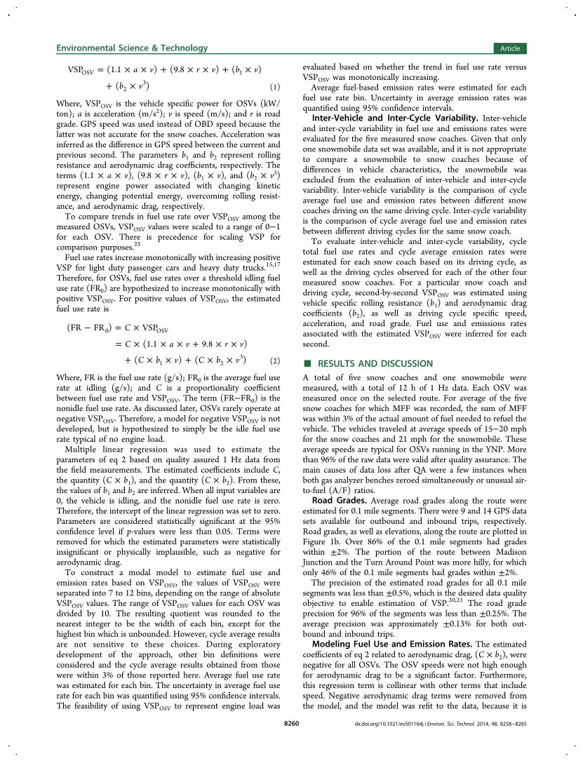
Where, VSPOSV is the vehicle specific power for OSVs (kW/ton); a is acceleration (m/s2); v is speed (m/s); and r is roadgrade. GPS speed was used instead of OBD speed because thelatter was not accurate for the snow coaches. Acceleration wasinferred as the difference in GPS speed between the current andprevious second. The parameters b1 and b2 represent rollingresistance and aerodynamic drag coefficients, respectively. Theterms (1.1 × a × v), (9.8 × r × v), (b1 × v), and (b2 × v3)represent engine power associated with changing kineticenergy, changing potential energy, overcoming rolling resist-ance, and aerodynamic drag, respectively.To compare trends in fuel use rate over VSPOSV among the

measured OSVs, VSPOSV values were scaled to a range of 0−1for each OSV. There is precedence for scaling VSP forcomparison purposes.25

Fuel use rates increase monotonically with increasing positiveVSP for light duty passenger cars and heavy duty trucks.15,17

Therefore, for OSVs, fuel use rates over a threshold idling fueluse rate (FR0) are hypothesized to increase monotonically withpositive VSPOSV. For positive values of VSPOSV, the estimatedfuel use rate is

− = ×

= × × × + × ×

+ × × + × ×

C

C a v r v

C b v C b v

(FR FR ) VSP

(1.1 9.8 )

( ) ( )

0 OSV

1 23

(2)

Where, FR is the fuel use rate (g/s); FR0 is the average fuel userate at idling (g/s); and C is a proportionality coefficientbetween fuel use rate and VSPOSV. The term (FR−FR0) is thenonidle fuel use rate. As discussed later, OSVs rarely operate atnegative VSPOSV. Therefore, a model for negative VSPOSV is notdeveloped, but is hypothesized to simply be the idle fuel userate typical of no engine load.Multiple linear regression was used to estimate the

parameters of eq 2 based on quality assured 1 Hz data fromthe field measurements. The estimated coefficients include C,the quantity (C × b1), and the quantity (C × b2). From these,the values of b1 and b2 are inferred. When all input variables are0, the vehicle is idling, and the nonidle fuel use rate is zero.Therefore, the intercept of the linear regression was set to zero.Parameters are considered statistically significant at the 95%confidence level if p-values were less than 0.05. Terms wereremoved for which the estimated parameters were statisticallyinsignificant or physically implausible, such as negative foraerodynamic drag.To construct a modal model to estimate fuel use and

emission rates based on VSPOSV, the values of VSPOSV wereseparated into 7 to 12 bins, depending on the range of absoluteVSPOSV values. The range of VSPOSV values for each OSV wasdivided by 10. The resulting quotient was rounded to thenearest integer to be the width of each bin, except for thehighest bin which is unbounded. However, cycle average resultsare not sensitive to these choices. During exploratorydevelopment of the approach, other bin definitions wereconsidered and the cycle average results obtained from thosewere within 3% of those reported here. Average fuel use ratewas estimated for each bin. The uncertainty in average fuel userate for each bin was quantified using 95% confidence intervals.The feasibility of using VSPOSV to represent engine load was

evaluated based on whether the trend in fuel use rate versusVSPOSV was monotonically increasing.Average fuel-based emission rates were estimated for each

fuel use rate bin. Uncertainty in average emission rates wasquantified using 95% confidence intervals.

Inter-Vehicle and Inter-Cycle Variability. Inter-vehicleand inter-cycle variability in fuel use and emissions rates wereevaluated for the five measured snow coaches. Given that onlyone snowmobile data set was available, and it is not appropriateto compare a snowmobile to snow coaches because ofdifferences in vehicle characteristics, the snowmobile wasexcluded from the evaluation of inter-vehicle and inter-cyclevariability. Inter-vehicle variability is the comparison of cycleaverage fuel use and emission rates between different snowcoaches driving on the same driving cycle. Inter-cycle variabilityis the comparison of cycle average fuel use and emission ratesbetween different driving cycles for the same snow coach.To evaluate inter-vehicle and inter-cycle variability, cycle

total fuel use rates and cycle average emission rates wereestimated for each snow coach based on its driving cycle, aswell as the driving cycles observed for each of the other fourmeasured snow coaches. For a particular snow coach anddriving cycle, second-by-second VSPOSV was estimated usingvehicle specific rolling resistance (b1) and aerodynamic dragcoefficients (b2), as well as driving cycle specific speed,acceleration, and road grade. Fuel use and emissions ratesassociated with the estimated VSPOSV were inferred for eachsecond.

■ RESULTS AND DISCUSSIONA total of five snow coaches and one snowmobile weremeasured, with a total of 12 h of 1 Hz data. Each OSV wasmeasured once on the selected route. For average of the fivesnow coaches for which MFF was recorded, the sum of MFFwas within 3% of the actual amount of fuel needed to refuel thevehicle. The vehicles traveled at average speeds of 15−20 mphfor the snow coaches and 21 mph for the snowmobile. Theseaverage speeds are typical for OSVs running in the YNP. Morethan 96% of the raw data were valid after quality assurance. Themain causes of data loss after QA were a few instances whenboth gas analyzer benches zeroed simultaneously or unusual air-to-fuel (A/F) ratios.

Road Grades. Average road grades along the route wereestimated for 0.1 mile segments. There were 9 and 14 GPS datasets available for outbound and inbound trips, respectively.Road grades, as well as elevations, along the route are plotted inFigure 1b. Over 86% of the 0.1 mile segments had gradeswithin ±2%. The portion of the route between MadisonJunction and the Turn Around Point was more hilly, for whichonly 46% of the 0.1 mile segments had grades within ±2%.The precision of the estimated road grades for all 0.1 mile

segments was less than ±0.5%, which is the desired data qualityobjective to enable estimation of VSP.20,21 The road gradeprecision for 96% of the segments was less than ±0.25%. Theaverage precision was approximately ±0.13% for both out-bound and inbound trips.

Modeling Fuel Use and Emission Rates. The estimatedcoefficients of eq 2 related to aerodynamic drag, (C × b2), werenegative for all OSVs. The OSV speeds were not high enoughfor aerodynamic drag to be a significant factor. Furthermore,this regression term is collinear with other terms that includespeed. Negative aerodynamic drag terms were removed fromthe model, and the model was refit to the data, because it is

Environmental Science & Technology Article

dx.doi.org/10.1021/es501164j | Environ. Sci. Technol. 2014, 48, 8258−82658260

physically impossible to have negative aerodynamic drag. Thus,the negative terms were removed even if they were statisticallysignificant.The estimated regression coefficients for fuel use versus

VSPOSV without aerodynamic drag are shown in Table 2. Allreported coefficients are statistically significant. The adjusted R2

coefficients of determination for all OSVs are at least 0.96,indicating a strong linear relationship.

The rolling resistance coefficient, b1, ranged from 1.9 to 5.5for the converted snow coaches. For these OSVs, the rollingresistance coefficients are an order of magnitude larger than fora typical highway light-duty vehicle, which has a typical value of0.132.18

For the dedicated OSVs, Bombardier, and the Arctic Cat, thevalues of the rolling resistance coefficients are much greaterthan for the converted highway vehicles, at 41, and 9.1,respectively. The tracks of the two dedicated OSVs have alarger ground contact area compared to the converted OSVs.Thus, a likely operational advantage of the dedicated OSVscompared to the converted highway vehicles is that they are lesslikely to slide.

Because of the high rolling resistance coefficients fordedicated OSVs, rolling resistance may be the dominant factoraffecting engine load. To explore this possibility, linearregression between nonidle fuel use rates and only the rollingresistance term were conducted for the Bombardier and theArctic Cat; results are shown in Table 2. The R2 coefficients ofdeterminations for the fuel use model based only on rollingresistance are nearly as high as those based on models that alsoinclude changes in kinetic and potential energy. Thus, rollingresistance alone is able to explain a large share of the variance ofdedicated OSV nonidle fuel use rates. Rolling resistance is aproperty of the vehicle, not of the terrain. The effect of roadgrade is accounted for separately from rolling resistance.Although the kinetic and potential energy terms are statisticallysignificant, they do not contribute much to the variance ofnonidle fuel use rates.To demonstrate the relationship between fuel use and engine

load, a plot of average fuel use rate versus VSPOSV bin is shownin Figure 2, using the Ford E350 snow coach as an example.

There were no VSPOSV values less than 0, because the OSVdriver typically coasts to a stop to avoid skidding, rather thanapplying the brakes. A monotonically increasing relationshipwas observed between fuel use rate and VSPOSV bins. Similarrelationships are observed for highway vehicles.24

For the other snow coaches, no negative VSPOSV values wereobserved except for the Ford F550 snow coach, which had only4 s of negative VSPOSV values. The relative trends between fueluse rates and VSPOSV for the other OSVs are similar to theE350, as shown in the SI. For each individual OSV, fuel userates are observed to increase linearly with VSPOSV. Therefore,VSPOSV is a useful parameter for representing OSV engine load.However, the magnitudes of fuel use rates are different

among the OSVs. The measured fuel economies for the OSVsare listed in Table 1. Among the five snow coaches, theBombardier typically had the lowest modal incremental nonidlefuel use rates, ranging from 0 to 5 g/s. The modal incrementalnonidle fuel use rates for the other four are similar, rangingfrom 0 to 10 g/s. The lighter chassis enabled the Bombardier tohave higher fuel economy than the converted snow coaches.The Arctic Cat has the lowest fuel use rates, because of a muchsmaller engine and lower weight.To evaluate emissions rates trends, examples of fuel-based

average CO and NOx emission rates versus fuel use rates for theFord E350 snow coach are shown in Figure 3. Fuel-based COemission rates increase with increasing fuel use rate initially,then decrease for fuel use bins ranging from 2 to 4 g/s, and

Table 2. Linear Regression Results of Non-Idling Fuel Useversus Kinetic and Potential Energy, and RollingResistancea,c

C (C × b1) b1

kinetic andpotential energycoefficientd

rollingresistance termcoefficientd

rollingresistance

over snowvehicle g-s2/m2 g/m m/s2

adjustedR2

Chevy Express 0.138 0.764 5.5 0.98Ford E350 0.279 0.541 1.9 0.98Ford F450 0.271 0.960 3.5 0.98Ford F550 0.554 0.816 1.5 0.98Bombardier 0.008 0.325 41 0.96Arctic CatTZ1

0.011 0.100 9.1 0.98

Bombardierb N/A 0.328 N/A 0.96Arctic CatTZ1b

N/A 0.103 N/A 0.97

aLinear regression for the first five rows is based on eq 2 excluding theaerodynamic drag term.

− = × × × + × ×

+ × ×

C a v r v

C b v

FR FR [(1.1 ) (9.8 )]

( )0

1

Where FR = fuel use rate (g/s), FR0 = average idling fuel use rate (g/s), v = speed (m/s), a = acceleration (m/s2), r = road grade (slope), C= regression coefficient for kinetic and potential energy (g-s2/m2), C ×b1 = regression coefficient for rolling resistance (g/m), and b1 = rollingresistance coefficient (m/s2). bLinear regression for these cases isbased on a simplified version of eq 2 that focuses only on rollingresistance as the dominant source of engine load:

− = × ×C b vFR FR ( )0 1

cAverage idling fuel use rate are 0.34, 0.36, 0.47, 0.37, 0.26, and 0.23g/s for the Bombardier, Chevrolet Express, Ford E350, Ford F450,Ford F550, and Arctic Cat TZ1, respectively. Sample size ranges from2000 s to 3240 s for each vehicle. dThe p-values for all coefficientestimates are less than 0.001.

Figure 2. Modal average fuel use rate versus scaled vehicle specificpower for over snow vehicles for the Ford E350 gasoline-fueled snowcoach. Error bars indicate 95% confidence intervals.

Environmental Science & Technology Article

dx.doi.org/10.1021/es501164j | Environ. Sci. Technol. 2014, 48, 8258−82658261

subsequently increase again. However, less than 3% of time wasspent in the bins with the decreasing emissions trend, which hastwo implications: (1) the decrease in emission rate at moderatefuel use rate does not have a substantial impact on cycleaverages; and (2) this trend may be an artifact of transientoperation. For all the bins, the exhaust HC concentrations weregenerally below the gas analyzer detection limit. Fuel-basedNOx emission rates generally increase with fuel use rates.

The modal average fuel-based CO emission rates for theBombardier were typically between 20 g/gallon and 60 g/gallon, with the exception of some data representing transientsat low fuel flow. In contrast, the Chevrolet Express had COemission rates that typically increased with fuel flow, with thehighest modal rate of over 1,000 g/gallon, more than a factor of5 higher than the next highest rate. For the two diesel OSVs,the average exhaust CO concentrations were below the gasanalyzer detection limit for all bins except for one bin for theFord F550. The low CO concentrations for the diesel OSVswere expected because diesel engines operate with excess air.For the Arctic Cat, fuel-based modal CO emission rates rangedfrom approximately 2000−2500 g/gallon for low to moderatefuel flow rate, and dropped to approximately 500 g/gallon athigh fuel flow rate.CO emissions can be produced as a result of incomplete

combustion. A gasoline A/F ratio less than 14.7 indicates fuelrich combustion.26 The A/F ratios of the Chevrolet and theArctic Cat were less than 14 for 66% and 46% of the time,respectively, compared to less than 1% of the time for theBombardier and the Ford E350. Thus, the high CO emissions

Figure 3. Average carbon monoxide and nitrogen oxide emission ratesin each fuel use bin for the Ford E350 gasoline-fueled snow coach.Error bars indicate 95% confidence intervals.

Table 3. Estimated Total Fuel Use and Cycle Average Carbon Monoxide and Nitrogen Oxides Emissions Rates for Each SnowCoach for Each Driving Cycle for the Out-Bound Trip

total fuel use (gallon)

driving cyclea

snow coach B CE E350 F450 F550inter-cycle H/L ratio ±st. dev cycle totalb

Bombardier (B) 3.5 3.4 3.4 3.5 3.4 1.05 ± 0.0003Chevy Express (CE) 7.8 7.5 7.6 7.7 7.5 1.04 ± 0.003Ford E350 (E350) 5.9 5.6 5.7 5.8 5.6 1.05 ± 0.0005Ford F450 (F450) 9.7 9.4 9.5 9.6 9.4 1.04 ± 0.0006Ford F550 (F550) 8.4 8.1 8.2 8.2 8.1 1.04 ± 0.0005

inter-vehicle H/L ratio ± st. dev vehicle totalc 2.7 ± 0.001 2.8 ± 0.001 2.8 ± 0.001 2.7 ± 0.001 2.8 ± 0.001cycle average CO emission rates (g/gallon)

.driving cycle

snow coach B CE E350 F450 F550inter-cycle H/L ratio ±

st. dev cycle avg

Bombardier (B) 36 40 40 39 41 1.14 ± 0.04Chevy Express (CE) 900 940 820 910 840 1.15 ± 0.01Ford E350 (E350) 39 34 32 34 32 1.20 ± 0.01Ford F450 (F450)d 1.1 3.7 4.3 3.4 4.5 n/aFord F550 (F550)d 0.8 0.1 0.4 0.6 0.1 n/a

inter-vehicle H/L ratio ± st. dev vehicle avg.e 25 ± 0.61 27 ± 0.29 26 ± 0.30 26 ± 0.28 26 ± 0.31cycle average NOx emission rates (g/gallon)

driving cycle

snow coach B CE E350 F450 F550inter-cycle H/L ratio ±

st. dev cycle avg

Bombardier (B) 24 30 30 28 30 1.27 ± 0.02Chevy Express (CE) 9.6 10 9.0 9.6 9.2 1.10 ± 0.03Ford E350 (E350) 0.8 0.8 0.7 0.7 0.7 1.08 ± 0.02Ford F450 (F450) 23 22 22 22 22 1.06 ± 0.01Ford F550 (F550) 12 14 14 13 14 1.17 ± 0.04

inter-vehicle H/L ratio ± st. dev vehicle avg. 31 ± 0.46 39 ± 0.61 42 ± 0.70 38 ± 0.60 41 ± 0.69

aDriving cycle: B = Bombardier driving cycle; CE = Chevrolet Express driving cycle; E350 = Ford E350 driving cycle; F450 = Ford F450 drivingcycle; F550 = Ford F550 driving cycle. bH/L ratio cycle total = Ratio of highest to lowest cycle total rates; For example, for Bombardier, for fuel usetotal, H/L ratio cycle total of 1.05 is obtained by 3.5 gallons divided by 3.4 gallons. cH/L ratio vehicle total/Avg. = Ratio of highest to lowest vehicletotal or average rates. For example, for Bombardier, for fuel use total, H/L ratio vehicle total of 2.8 is obtained by 9.7 gallons divided by 3.5 gallons.dValues in italics are below the detection limit and are not included in the H/L ratio. eThe H/L ratios are calculated only using values above thedetection limit.

Environmental Science & Technology Article

dx.doi.org/10.1021/es501164j | Environ. Sci. Technol. 2014, 48, 8258−82658262

for the Chevrolet and the Arctic Cat were attributed to fuel richoperation.The average exhaust HC concentrations for the Bombardier,

Ford F450 and F550 were below the gas analyzer detectionlimit for all bins. Therefore, there was typically no identifiabletrend in HC emission rates for these snow coaches. For theChevrolet Express, the average exhaust HC concentrationswere below the detection limit for all except the highest fuelflow bins. For the Arctic Cat, the exhaust HC concentrationswere above the detection limit, and the fuel-based HC emissionrates generally decreased with fuel use rates. Thus, the HCemission rates were generally low except for the two OSVs thathad substantial portions of time with fuel-rich engine operation.A generally increasing trend of fuel-based NOx emission rates

versus fuel use rate was observed for the gasoline-fueledBombardier, Chevrolet, and Arctic Cat. Based on the Zeldovichmechanism, engine-out NOx emission rates typically increasewith engine load because of increasing peak flame temperaturesin the engine cylinders during the power stroke.26 The NOxemission rate for the E350 was very low compared to all othervehicles. For the diesel-powered Ford F450 and Ford F550with SCR, the fuel-based NOx emission rates were not sensitiveto fuel use rate. SCR is effective at controlling NOx, since theobserved emission rates are approximately 66% lower than thediesel OSV measured previously in 2006.11 In addition, themeasured NOx emission rates were comparable to those of thegasoline vehicles, which would not have been the case withoutSCR. However, for diesel OSVs equipped with SCR and DPF,the NO to NOx ratio in the exhaust could decrease toapproximately 0.7, compared to approximately 0.95 when notequipped with SCR and DPF.27 If this decreased NO/NOxratio is used, the NOx emission rates for the diesel OSVs wouldincrease by approximately 30%.For PM emissions from the diesel OSVs with DPF, no trend

was observed with respect to fuel use rate. The opacity-basedPM emission rates were below 0.1 g/gallon for all fuel use bins.These rates are very low and are consistent with DPFoperation. The PM emission rates for OSVs with DPFs arecomparable to highway vehicles with DPFs.22

For the measured three gasoline snow coaches, the cycleaverage HC and NOx emission rates were 85% and 65% lower,respectively, compared to the gasoline snow coaches measuredin 2006.11 The average CO emission rate was 17% higher, butthe rate would be 92% lower if excluding the high CO emittingChevrolet Express. For the two diesel OSVs, the PM, CO, andNOx emission rates were lower by 97%, 86%, and 66%,respectively, compared to the diesel OSV measured in 2006.11

The general lower emissions for the recently measured vehiclesare mainly attributed to more stringent emission controlscompared to older model year vehicles measured in prior work.This is the first time that a relationship between engine load,

fuel use, and emission rates have been developed for OSVs,taking into account speed, acceleration and road grade, that canbe used for any real-world driving cycle. VSP can be adapted tovehicle types other than highway vehicles, thereby enablingdevelopment of VSP-based modal models that can be used topredict cycle average emissions for specific combinations ofvehicles and driving cycles. Such models can supportdevelopment of vehicle emissions estimates with high spatialand temporal resolution, which in turn are useful for emissioninventories, air quality modeling, exposure assessment, andother applications.

Inter-Vehicle and Inter-Cycle Variability. Results forinter-vehicle and inter-cycle variability for the five measuredsnow coaches, in terms of total fuel use and cycle averageemission rates of CO, and NOx, are given in Table 3. This tableincludes results for the out-bound trip. The results for the in-bound trip, provided in the SI, were similar to the out-boundtrip. Because the exhaust HC concentrations were typicallybelow the detection limit, cycle average HC emission rates arenot included.For fuel use, the value in each cell of Table 3 is the estimated

total fuel use for a given OSV on a given cycle. For example, forthe Bombardier simulated on the Chevrolet Express drivingcycle, the estimated total fuel use is 3.4 gallons. Likewise, theestimated cycle average CO and NOx emission rates are 40 gper gallon and 30 g per gallon, respectively.To quantify inter-vehicle variability, for a given driving cycle,

the ratio of the highest to lowest rates (H/L ratio) wasestimated. For example, for the Bombardier cycle, the highesttotal fuel use is 9.7 gallons from the Ford F450 and the lowestis 3.5 gallons from the Bombardier. Therefore, the H/L ratio is2.8. For the other driving cycles, the H/L ratios were similar,ranging from 2.7 to 2.8. Differences in vehicle weight, tracktype, and engine characteristics are key reasons for thevariability.There is inter-vehicle variability in cycle average CO and

NOx emission rates among the five OSVs, with H/L ratios of25−27 for CO and 31−42 for NOx. The CO emission rates forthe two diesel vehicles were below the detection limit and arenot included in the H/L ratio. Even though the precise COemission rate for the diesels is not quantifiable, it is clear thatthe diesels have much lower CO emissions than the gasolineOSVs.Inter-cycle variability for a given OSV is quantified based on

the H/L ratio among different driving cycles. Differences intotal fuel use from different driving cycles are within 5%. Forcycle average CO and NOx emissions, the differences fromdifferent driving cycles are within 30%, excluding the F450 andF550 CO emission rates which were below the detection limit.Therefore, the inter-cycle variability has limited effect on totalfuel use.For PM emissions for the two diesel OSVs, the inter-vehicle

H/L ratios are approximately 1.4, as detailed in the SI. The PMemissions were low due to the equipped DPF. The inter-cycleH/L ratios are approximately 1.1. Both inter-vehicle and inter-cycle variability have only moderate effect on cycle average PMemission rates.The standard deviations of the H/L ratios were estimated, as

shown in Table 3. All of the H/L ratios are statisticallysignificantly different than 1.Prior to this work, little was known as to whether differences

in driving cycles might lead to substantial differences in fuel useand emission rates for OSVs. The observed driving cycles arebased on different vehicles and different drivers. The similarityin the cycle average rates may be a result of the dominance ofrolling resistance as a factor determining engine load. Whileone might posit the possibility of “alternate” driving cycles thatcould produce different cycle average rates, OSV operation isconstrained by the preference to avoid skidding or slippage,thus limiting acceleration and deceleration rates. It is not likely,therefore, that there many alternate cycles to those observedthat would also be consistent with safe operation. The findingthat cycle average rates are robust to inter-cycle variability isuseful in that it implies there is not as much need to consider

Environmental Science & Technology Article

dx.doi.org/10.1021/es501164j | Environ. Sci. Technol. 2014, 48, 8258−82658263

multiple cycles for OSVs, which differs from other types ofvehicles such as highway vehicles.The VSP-based approach here enables comparisons of

multiple vehicles for the same cycle, thereby enabling bettercomparison of inter-vehicle variability in fuel use and emissionrates, such as because of fuel (e.g., gasoline, diesel) or emissioncontrol technologies. Furthermore, the approach here enablesquantitative assessment of the extent to which variabilitybetween driving cycles leads to variability in fuel use andemission rates. In past work, it was not possible to separate theeffect of driving cycles, which inherently vary from one test toanother, from inter-vehicle variability. The approach demon-strated here enables more clear insight regarding the variabilityin fuel use and emission rates associated with driving cycles,which are depending on activity patterns, as distinct frommodal fuel use and emission rates specific to a vehicle, whichare depending on vehicle fuel and technology.The results obtained here can be used to estimate how many

vehicles need to be sampled to achieve a target data qualityobjective for uncertainty in fleet average emission rates. TheOSV inter-vehicle variability in fuel use and emissions was large.Assuming the same sample average and standard deviation asfor the five measured snow coaches, a sample size of 15 vehiclesfor fuel use and 100 vehicles for NOx emissions is required tobound the 95% confidence interval to within ±20% of themean.Data collection for this study was conducted for only 2

weeks. Therefore, it was not possible to observe variability in allfactors that could affect OSV fuel use and emission rates, suchas snow condition and passenger load. It is hypothesized thatthe snow condition, such as whether loose or packed, has asignificant effect on the rolling resistance and, therefore, affectsfuel use and emissions rates. There is evidence that loose snowmight lead to a significant increase in CO and HC emissionrates.11

Based on previous OSV studies, the effect of passenger loadwas inferred to be less significant than the effect of snowconditions.11 However, passenger load was found to have asignificant effect on fuel use and emissions for other types ofvehicles, such as transit buses.15 For the Ford E350, the curbweight is approximately 6400 lb, and the passenger capacity is15. Assuming 200 lb per passenger, the fully loaded weightcould be approximately 50% greater than for an empty van, andthus, might lead to significant increase in fuel use and emissionrates.Activity data should be collected over a longer time period

for a selected set of OSVs to enable assessment of the effect ofsnow conditions and passenger load on fuel use. The activitydata needed include 1 Hz fuel use rate, speed, acceleration, androad grade. These data could be accessed using the OBDinterface and GPS/BA receivers only. Using the methodintroduced in this study, the rolling resistance coefficients couldsimilarly be quantified under selected combinations of snowand passenger load conditions. If fuel use rates are found to besubstantially affected by these factors, a future study couldadditionally target emission measurements. Such data wouldsupport development of improved winter use plans.The methods demonstrated here can be applied to other

OSVs. The general form of the regression models is broadlyapplicable to OSVs. The values of the regression coefficientsmay be specific to combinations of vehicles and snowconditions, which should be investigated in further workusing simplified activity data collection methods described

above. However, vehicle models of fuel use and emissions canbe calibrated with a limited amount of PEMS data.Furthermore, a limited sample of vehicles is sufficient toquantify a fleet average with a desired degree of precision. Incontrast, vehicle activity data can be collected less expensivelyand therefore more extensively, than emissions data. Using themodeling approach demonstrated here, it is possible to estimateOSV fuel use and emissions for a variety of road segmentstaking into account speed, acceleration, and road grade.

■ ASSOCIATED CONTENT*S Supporting InformationAdditional description of the measured vehicles, additionaldetails regarding the study route, additional details regardingmethods for instrument calibration and validation, and for datasynchronization, quality assurance and analysis; linear regres-sion results for nonidling fuel use versus kinetic and potentialenergy, rolling resistance, and aerodynamic drag; figures ofaverage fuel use in VSPOSV bins for selected OSVs; figures ofaverage emissions rates in fuel use bins for selected OSVs;average emissions rates in predicted fuel use bins; inter-vehicleand inter-cycle variability for fuel use and emissions rates forselected OSVs; fuel use comparison for each snow coach; andcumulative probabilities of speed, acceleration, and road gradefor selected driving cycles. This material is available free ofcharge via the Internet at http://pubs.acs.org/.

■ AUTHOR INFORMATIONCorresponding Author*Phone: 919-515-1155; fax: 919-515-7908; e-mail: frey@ncsu.edu.NotesThe authors declare no competing financial interest.

■ ACKNOWLEDGMENTSThe field measurements were sponsored by the National ParkService of the U.S. Department of the Interior via Louis BergerGroup, Inc. in Denver, Colorado. Numerous vehicle ownersand operators provided logistical support for this project,including access to and operation of the OSVs during datacollection.

■ REFERENCES(1) U.S. District Court for the District of Columbia December 16,2003 Ruling; available at http://www.nps.gov/yell/parkmgmt/upload/12_16opinion-2.pdf (accessed 2014).(2) U.S. District Court for Wyoming February 10, 2004 Ruling;available at http://www.nps.gov/yell/parkmgmt/upload/brimmer_order.pdf (accessed 2014).(3) NPS. Winter Use Plans: Final Environmental Impact Statement forthe Yellowstone and Grand Teton National Parks and John D. Rockefeller,Jr. Memorial Parkway; National Park Service: Lakewood, CO, 2000.(4) NPS. Temporary Winter Use Plans Environmental Assessment; U.S.Department of Interior; National Park Service: Lakewood, CO, 2004;avai lable at http://www.nps.gov/yell/parkmgmt/upload/tempwinteruseea8-18.pdf (accessed 2014).(5) NPS. Best available technology (BAT). Fed. Regist., November 20,2009, 74 (223), 60159.(6) NPS. Snowmobile Best Available Technology (BAT) List; NationalPark Service: Lakewood, CO, 2009; available at http://www.nps.gov/yell/parkmgmt/current_batlist.htm (accessed 2014).(7) NPS. Yellowstone in Winter: Current Management and Planning;National Park Service: Lakewood, CO, 2012; available at http://www.nps.gov/yell/parkmgmt/currentmgmt.htm (accessed 2014).

Environmental Science & Technology Article

dx.doi.org/10.1021/es501164j | Environ. Sci. Technol. 2014, 48, 8258−82658264

(8) Frey, H. C., Sandhu, G. S., Graver, B. M., Hu, J. Measurement ofFuel Use and Emissions of Over-Snow Vehicles at Yellowstone NationalPark; Final Report prepared by North Carolina State University forLouis Berger Group: Denver, CO, August, 2012.(9) Ray, J. D., Bishop, G.; Schuchmann, B.G.; Frey, H.C.; Sandhu,G.S.; , and Graver, B.M.; Yellowstone Over-snow Vehicle Emission Tests −2012: Summary Vehicle Data and Fleet Estimates for Modeling, NaturalResource Technical Report NPS/NRPC/ARD/NRTR − 2012. DraftV6.5; National Park Service: Fort Collins, CO, 2012.(10) Bishop, G. A.; Burgard, D. A.; Dalton, T. R.; Stedman, D. H.;Ray, J. D. Winter motor-vehicle emissions in Yellowstone NationalPark. Environ. Sci. & Technol. 2006, 40 (8), 2505−2510.(11) Bishop, G. A.; Stadtmuller, R.; Stedman, D. H.; Ray, J. D.Portable emission measurements of snowcoaches and snowmobiles inYellowstone National Park. J. Air Waste Manage. Assoc. 2009, 59 (8),936−942.(12) Bishop, G. A.; Stedman, D. H.; Hektner, M.; Ray, J. D. An in-usesnowmobile emission survey in Yellowstone National Park. Environ.Sci. & Technol. 1999, 33 (21), 3924−3926.(13) Unal, A.; Frey, H. C.; Rouphail, N. M. Quantification of highwayvehicle emissions hot spots based upon on-board measurements. J. AirWaste Manage. Assoc. 2004, 54 (2), 130−140.(14) Frey, H. C.; Kim, K. Comparison of real-world fuel use andemissions for dump trucks fueled with B20 biodiesel versus petroleumdiesel. Transp. Res. Rec. 2006, 1987, 110−117.(15) Frey, H. C.; Rouphail, N. M.; Zhai, H.; Farias, T. L.; Gonca̧lves,G. A. Modeling and comparing real-world fuel consumption for diesel-and hydrogen-fueled transit buses and implication for emissions.Transp. Res., Part D 2007, 12, 281−291.(16) Wang, H.; Fu, L.; Zhou, Y.; Li, H. Modeling of the fuelconsumption for passenger cars regarding driving characteristics.Transp. Res., Part D 2008, 13 (7), 479−482.(17) Zhai, H.; Frey, H. C.; Rouphail, N. M. A Vehicle-specific powerapproach to speed- and facility- specific emissions estimates for dieseltransit buses. Environ. Sci. Technol. 2008, 42 (21), 7985−7991.(18) Jimenez-Palacios, J. Understanding and quantifying motorvehicle emissions and vehicle specific power with TILDAS remotesensing, Doctoral Dissertation, Massachusetts Institute of Technology,1999.(19) Frey, H. C.; Zhang, K.; Rouphail, N. M. Fuel use and emissionscomparisons for alternative routes, time of day, road grade, andvehicles based on in-use measurements. Environ. Sci. Technol. 2008, 42(7), 2483−2489.(20) Yazdani, B.; Frey, H. C. Road grade quantification based onglobal positioning system data obtained from real-world vehicle fueluse and emission measurements,. Atmos. Environ. 2014, 85, 179−186.(21) Yazdani, B.; Frey, H. C.; Sandhu, G. S. In-vehicle road grademeasurement using stand-alone GPS with barometric altimeter. J.Transp. Eng. 2013, 139 (6), 605−611.(22) Sandhu, G. S.; Frey, H. C. Real-world measurement andevaluation of duty cycles, fuels, and emission control technologies ofheavy-duty trucks. J. Transp. Res. Board 2012, 2270, 180−187.(23) Hendricks, E. and Sorenson, S.C.; SI Engine Controls and MeanValue Engine Modelling, SAE Technical Papers; Number 910258; SAEInternational, 1991.(24) Sandhu, G. S.; Frey, H. C. Effects of errors on vehicle emissionrates from portable emissions measurement systems. Transp. Res. Rec.2013, 2340, 10−19.(25) USEPA. MOVES2010 Highway Vehicle: Population and ActivityData, Final Report EPA-420-R-10-026; U.S. Environmental ProtectionAgency, Office of Transportation and Air Quality: Ann Arbor, MI,2010.(26) Heywood, J. B. Internal Combustion Engine Fundamentals;McGraw-Hill: New York, 1988.(27) Dallmann, T. R.; DeMartini, S. J.; Kirchstetter, T. W.; Herndon,S. C.; Onasch, T. B.; Wood, E. C.; Harley, R. A. On-road measurementof gas and particle phase pollutant emission factors for individualheavy-duty diesel trucks. Environ. Sci. Technol. 2012, 46, 8511−8518.

Environmental Science & Technology Article

dx.doi.org/10.1021/es501164j | Environ. Sci. Technol. 2014, 48, 8258−82658265