Mendelian Randomisation as an Instrumental …chambaz/Atelier209/12...Mendelian Randomisation as an...

Mendelian Randomisation as an Instrumental

Variable Approach to Causal Inference

Vanessa Didelez

School of Mathematics

University of Bristol

MRC project “Inferring epidemiological causality using Mendelian randomisation ”With T.Palmer, N.Sheehan, S.Meng, R.Harbord, F.Windmeijer, J.Stern, D.Lawlor,

G.Davey Smith

Bordeaux, June 2011

Based on:

Didelez, Sheehan (2007). Mendelian randomisation as an instrumental variableapproach to causal inference. Statistical Methods in Medical Research, 16, 309-330.

Didelez, Sheehan (2007). Mendelian randomisation: why epidemiology needs aformal language for causality. In: F.Russo and J.Williamson (eds.), Causality andProbability in the Sciences, College Publications London.

Didelez, Meng, Sheehan (2010). Assumptions of IV Methods for ObservationalEpidemiology. Statistical Science 25, 22-40.

Palmer, Sterne, Harbord, Lawlor, Sheehan, Meng, Granell, DaveySmith, Didelez (2011). Instrumental variable estimation of the causal risk ratioand causal odds ratio in Mendelian randomization analyses. American Journal ofEpidemiology, 173(12), 1392-1403. DOI: 10.1093/aje/kwr026

Overview

• Part 1: Mendelian Randomisation and Instrumental Variables

• Part 2: A Closer Look at the IV Assumptions

• Part 3: Unsing IV to Estimate a Causal Effect

Part 1:

Mendelian Randomisation and Instrumental Variables

• Motivation and basic idea

• Example: effect of alcohol consumption on health outcome using

ALDH2 genotype

• Formal definition of IV

1

Motivation

Epidemiology interested in effect of interventions (‘drink less alcohol’,

‘eat folic acid’ etc.)

Observational studies are inevitable: preliminary research, but also

assessment of effects in general population.

Obvious problem is confounding: effects of interest are entangled with

many other effects — this can never be fully excluded.

Instrumental variables allow some inference on effects of interventions

in the presence of confounding.

Problem with this is: how to find a suitable instrument? It has recently

become popular to look for a genetic variant as IV — Mendelian

randomisation.

2

Motivation






many other effects — this can never be fully excluded. Example





randomisation.

2

Example: Alcohol Consumption

Alcoholconsumption

Disease

unobservedLifestyle /

confounders

?

Chen et al. (2008)

Alcohol consumption has been found in observational studies to have

positive ‘effects’ (coronary heart disease) as well as negative ‘effects’

(liver cirrhosis, some cancers, mental health problems).

But also strongly associated with all kinds of confounders (lifestyle etc.),

as well as subject to self–report bias. Hence doubts in causal meaning

of above ‘effects’.

3

Motivation ctd.






many other effects — this can never be fully excluded.





randomisation.

4

Mendelian Randomisation: Basic Idea

Idea: if we cannot randomise, let’s look for instances where ‘nature’

has randomised, e.g. through genetic variation.


Genotype: ALDH2 determines blood acetaldehyde, the principal

metabolite for alcohol.

Two alleles/variants: wildetype *1 and “null” variant *2.

*2*2 homozygous individuals suffer facial flushing, nausea, drowsiness

and headache after alcohol consumption.

⇒ *2*2 homozygous individuals have low alcohol consumption

regardless of their other lifestyle behaviours

IV–Idea: check if these individuals have a different risk than others for

alcohol related health problems!

5

Effect of Interventions — Formally

Want notation to distinguish between association and causation.

Intervention: setting X to a value x denoted by σX = x.

p(y;σX = x) not necessarily the same as p(y|X = x;σX = ∅).

• p(y;σX = x), if it depends on x then regard X as causal for Y

⇒ typically observed in a randomised study.

Note: this is a total (or population) effect.

• p(y|X = x;σX = ∅) will also depend on x when there is confounding,

reverse causation etc.

⇒ typically observed in an observational study.

Note: for simple intervention we often use Pearl’s do(X = x) notation.

6

Definition of IV

YG X

U

Xσ

Definition of instrumental variable

1. G⊥⊥U | σX = ∅

2. G⊥⊥/ X | σX = ∅

3. G⊥⊥Y | (X,U, σX = ∅).

And if the following structural assumptions are valid:

Y⊥⊥σX|(X,U), G⊥⊥σX and U⊥⊥σX.

7

Instrumental Variables — Graphically

YG X

U

Xσ

Equivalent to factorisation

p(y, x, u, g;σX) = p(y|x, u)p(x|u, g;σX)p(u)p(g)

8

Instrumental Variables — Graphically

YG X

U

xX

=σ

With structural assumption: under intervention in X

p(y, u, g;σX = x̃) = p(y|x̃, u;σX = ∅)p(u)p(g)

Note 1: implies Y⊥⊥G | σX 6= ∅ – also known as exclusion restriction.

Note 2: exclusion restriction does not refer to U .

9

Why does IV Help with Causal Inference?

Testing:

check if Y⊥⊥G — this is (roughly) testing whether there is a causal

effect at all.

Estimation:

(1) when all observable variables are discrete, we can obtain bounds on

causal effects without further assumptions.

(2) for point estimates need some (semi–)parametric / structural

assumptions, as well as clear definition of target causal parameter.

10

Part 2:

A Closer Look at the IV Assumptions

• How can we justify the assumptions?

• Usign IV to test for a causal effect

• Possible violations of the IV

11

‘Untestable’ Assumptions

The assumptions

1. G⊥⊥U

3. G⊥⊥Y | (X,U).

impose inequality constraints when X,Y,G discrete.

They do not imply that G⊥⊥Y |X or G⊥⊥Y !

⇒ Need to be justified based on subject matter background knowledge.

⇒ Mendelian randomisation

12


Alcoholconsumption

DiseaseALDH2genotype


confounders

?

(1)

(2)

Note 1: due to random allocation of genes at conception, can be fairly

confident that genotype is not associated with unobserved confounders

(subpopulation structure can be a problem).

Further evidence: in extensive studies no evidence for association with

observed confounders, e.g. age, smoking, BMI, cholesterol.

(see also Davey Smith et al., 2007)

13


Alcoholconsumption



confounders

?

(1)

(2)

Note 2: due to known ‘functionality’ of ALDH2 gene, we can exclude

that it affects the typical diseases considered by another route than

through alcohol consumption.

⇒ important to use well studied genes as instruments!

14


Alcoholconsumption



confounders

?(3)

Note 3: association of ALDH2 with alcohol consumption well

established, strong, and underlying biochemistry well understood.

15


0

10

20

30

40

2*2/2*2 2*2/2*1 1*1/1*1

Alc

ohol

inta

ke m

l/da

y

ALDH2 genotype

Note 3: association of ALDH2 with alcohol consumption well

established, strong, and underlying biology well understood.

16

Using IV to Test for Causal Effect

U

YG X

simply test if

Y⊥⊥G

i.e. independence between

instrument and outcome

Message: regardless of measurement level, testing Y⊥⊥G is valid test

for presence of causal effect of X on Y ;

no further parametric assumptions required!

(Exception to the rule: if U acts as effect modifier in a very specific way.)

17


Alcoholconsumption



confounders

?

Causal Effect? under IV assumptions, the null–hypothesis of no causal

effect of alcohol consumption, should imply no association between

ALDH2 and disease;

While if alcohol consumption has a causal effect we would expect an

association between ALDH2 and disease.

18


Findings: (Meta-analysis by Chen et al., 2008)

Blood pressure on average 7.44mmHg higher and

risk of hypertension 2.5 higher

for ALDH2*1*1 than for ALDH2*2*2 carriers (only males).

⇒ mimics the effect of large versus low alcohol consumption.

Blood pressure on average 4.24mmHg higher and

risk of hypertension 1.7 higher

for ALDH2*1*2 than for ALDH2*2*2 carriers (only males).

⇒ mimics the effect of moderate versus low alcohol consumption.

⇒ it seems that even moderate alcohol consumption is harmful.

Note: studies mostly in Japanese populations (where ALDH2*2*2 is

common), where women drink only little alcohol in general.

19


(Chen et al., 2008)

Is condition Y⊥⊥G|(X,U) satisfied?

Some indication

Women in Japanese study population do not drink. ALDH2 genotype

in women not associated with blood pressure ⇒ there does not seem to

be another pathway creating a G–Y association here.

20

Violations of Core Conditions

So far have argued that in Mendelian randomisation studies we can

reasonably believe that core conditions are satisfied.

Now will discuss situations and examples when they are typically violated.

(Davey Smith & Ebrahim, 2003)

Use graphs to represent assumptions / background knowledge to check

if core conditions are violated or not.

21

Population Stratification

Population stratification occurs when there exist population subgroups

that experience both, different disease rates (or different distributions

of phenotypes) and have different frequencies of alleles of interest.

⇒ might violate condition Y⊥⊥G|(X,U).

22

Population Stratification (1)

Graphical representation:

variable P = population predicts G as well as Y

P

YG X

U

Here Y⊥⊥/ G|(X,U)!

⇒ can be avoided by sensible study design.

23


Example: Study of native Americans from Pima and Papago tribe.

(Knowler et al, 1988)

• Strong inverse association between a HLA–haplotype and type 2

diabetes;

• Individuals with full American Indian heritage: haplotype prevalence

1% and type 2 diabetes prevalence 40%;

• In Caucasian population: haplotype prevalence 66% and type 2

diabetes prevalence 15%.

⇒ Solution: carry out analyses within population strata!

• Note: need to be aware of existence of such population subgroups.

24


Also possible: phenotype distribution different in subgroups

P

YG X

U

Core conditions still satisfied.

Strength of IV could be affected in positive or negative way.

25

Linkage Disequilibrium (1)

Linkage disequilibrium (LD): is the correlation between allelic states at

different loci, traditionally regarded as stemming from close proximity

to each other on chromosome.

If genetic variant chosen as instrument is in LD with another gene

that is in turn associated with some of the unobserved confounders or

even predicts the disease, then condition Y⊥⊥G|(X,U) might again be

violated.

26


Graphical representation: G1 = chosen instrument, in LD with other

gene G2 through parental genes P .

YX

UG2

G1

P

Here Y⊥⊥/ G|(X,U) or G⊥⊥/ U !

27


‘Right’ gene?

Often it is plausible that the gene chosen as instrument is not the causal

gene for the phenotype of interest, but instead it is in LD with the

causal gene.

We could also regard this as measurement error when assessing the

gene.

This does not necessarily imply any violations of the core IV conditions.

⇒ we do not need to use the causal gene for Mendelian randomisation,

just one that is correlated with the phenotype, as long as core conditions

satisfied.

28


Chosen gene G1 is not ‘causal’

YX

UG2

G1

Core conditions still satisfied.

Again, strength of IV could be affected.

29

Pleiotropy

Peiotropy refers to a genetic variant having multiple functions, i.e. the

chosen gene / instrument might not only affect the phenotype of interest

but also other traits.

If the pleiotropic effects influence or predict the outcome through other

pathways, then the IV core conditions might again be violated.

30

Pleiotropy


G affects another phenotype X2 (phenotype of interest is X1)

Y

U

G

X2

X1

Here, again, Y⊥⊥/ G|(X,U) or G⊥⊥/ U .

31

Pleiotropy

Example: use of APOE genotype as IV for causal effect of both types

of cholesterol (HDLc and LDLc) on myocardial infarction risk.

• Causal effect of HDLc and LDLc well known from RCTs.

• APOE strongly associated with HDLc and LDLc, but surprisingly

APOE not associated with myocardial infarction risk.

• Explanation: the ǫ2 variant of APOE is also related to less efficient

transfer of very low-density lipoproteins and chylomicrons from the

blood to the liver, greater postprandial lipaemia, and an increased risk

of type III hyperlipoproteinaemia → all of which increase myocardial

infarction risk.

⇒ Due to multiple effects of APOE, all affecting myocardial infarction

risk, this is an unsuitable IV for a Mendelian randomisation study.

32

Genetic Heterogeneity

Genetic heterogeneity means that more than one genotype affect or

determine the phenotype of interest, possibly via different biochemical

routes.

To decide if this is a problem we need to establish whether these are in

LD and whether any of them have pleiotropic effects.

33



Independent genes affecting the phenotype.

YX

UG3

G1

G2

All core IV conditions still satisfied for each (or any subset of) genes.

34


Potential Benefits:

• Multiple instruments can be used to examine if the core conditions

are violated. If different genes affect the phenotype via different

pathways, it is unlikely that both are affected in the same way by

population stratification, LD or pleiotropy.

⇒ compare results obtained for each genotype separately.

• CRP example: circulating CRP is related to CRP–gene but also to

other locus, IL6, via different pathways.

• Can also combine multiple instruments for one IV analysis (common

in econometrics).

35

Measurement Errors

All measurements in a Mendelian randomisation study are prone to

measurement error.

In particular G: we often do not have the ‘right’ causal gene, but just

a strongly linked locus (cf. LD).

But G might also be mis-measured for other reasons ⇒ “in principle”

not a problem if measurement error not differential.

But might be a problem if G–X association is obtained from a different

study than G–Y association (meta analysis).

In practice, X is also typically measured with error. The ‘true’ phenotype

through which G acts is e.g. lifelong exposure to high or low CRP levels,

while what is measured is only the value at a particular time.

36

Measurement Errors


G∗ and X∗ are the actual measurements of G and X with possible

measurement errors.

U

YG X

G*

X*

Can use G∗ instead of G but not X∗ instead of X as G∗⊥⊥/ Y |(X∗, U).

Note: H0 ‘no causal effect’ can be tested by Y⊥⊥G regardless of X

37

Finding Genetic Instrumental Variable

Main limitation:

finding genetic variant that is suitable as instrumental variable!

Not many are known yet for typical exposures of interest in epidemiology.

Optimism: rapid expansion of knowledge in functional genomics!

Genome wide association studies:

gene–phenotype associations often weak, low power, not reproducible.

But even when strong/reproducible association found, functionality of

genes not well understood if only based on association studies.

⇒ cannot be as confident that core conditions satisfied.

Example: FTO genotype associated with BMI / fat mass but

functionality not (yet?) understood. (Frayling et al., 2007)

38

Example: FTO — fat/lean mass

From genome wide association studies:

39

Finding Genetic IV — Association Studies

Alternative explanation: G causes a

condition S, which in turn causes

the phenotype and disease of interest.Y

G

U

X

S

?

Here G⊥⊥/ X (genotype and phenotype are associated), G⊥⊥U .

But G⊥⊥/ Y |(X,U) — and cannot check this from data.

40

Part 3:

Using IV to Estimate Causal Parameters

• Target parameters

• Classical 2-stage-least-squares

• Methods for binary outcomes

• Application: effect of BMI on asthma in chlidren

41

Estimating Causal Parameters with IVs

There is a multitude of methods using an IV to obtain an estimate for

the causal effect of interest.

IV–based estimation methods differ in

– target causal parameter,

– model assumptions.

Will only consider a subjective selection of methods here.

42

Target Causal Parameters (1)

Population causal parameters:

Contrast between p(y;σX = x) for different values of x, e.g.

ACE average causal effect E(Y ;σX = x1)−E(Y ;σX = x0)

CRR causal risk ratio E(Y ;σX = x1)/E(Y ;σX = x0; )

or COR or...

Example: folic acid, hormone replacement therapy etc.

43


Effect of ‘treatment on the treated’ or ‘exposure on exposed’

Let X = ‘natural’ value of exposure (e.g. alcohol consumption)

and X∗ = exposure due to manipulation.

⇒ Contrast P (Y |X = x) ‘no intervention’

with P (Y |X = x;σX∗ = 0)) ‘enforcing baseline exposure’.

Example: make treatment available for those who want it, reduce

alcohol intake, etc.

⇒ target parameter of Structural Mean Models

44


Complier causal effect:

Target: E(Y1 − Y0|X1 > X0).

Definition ‘complier’ (X1 > X0):

if ‘set’ G = 0 then X = 0 and if ‘set’ G = 1 then X = 1.

Example: randomised trial with partial compliance, etc.

(Note: more complicated when X continuous.)

45

Typical Parametric Assumptions with IVs

Estimating a Causal Effect:

requires some additional parametric assumptions.

U

YG X

U

YG X

U

YG X

xX

=*

σ

Outcome models Exposure models Structural Mean models

E(Y |X,U) E(X|G,U) E(Y |X,G;σX∗ = x)

X → natural exp.

X̃ → manip. exp.

46

‘Classical’ IV Estimator

2–Stage–Least–Squares (2SLS): (or ratio / Wald estimator)

β̂IV =β̂Y |G

β̂X|G

• simple;

• only needs pairwise marginal data on (Y,G) and (X,G)

— could even come from separate data sets;

• generalises to multivariate X, Y and G:

predict X̂ from G, regress Y on X̂;

• consistent for ACE if...

47

Consistency of β̂IV

U

YG X

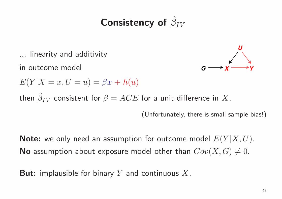
... linearity and additivity

in outcome model

E(Y |X = x,U = u) = βx + h(u)

then β̂IV consistent for β = ACE for a unit difference in X.

(Unfortunately, there is small sample bias!)

Note: we only need an assumption for outcome model E(Y |X,U).

No assumption about exposure model other than Cov(X,G) 6= 0.

But: implausible for binary Y and continuous X.

48

Something Similar for Binary Outcome Y ?

Suggestions for estimating CRR and COR (‘Wald–type’ estimators)

γ̂IV.RR =logRR(Y |G)

β̂X|G

η̂IV.OR =logOR(Y |G)

β̂X|G

But: need additional assumption about exposure model E(X|G,U).

Note: again, only needs pairwise marginal data on (Y,G) and (X,G)

— could come from separate data sets.

And, logOR(Y |G) could come from case–control study.

49

Consistency of γ̂IV.RR

U

YG X

Assume outcome model

logE(Y |X = x,U = u) = γx+ h(u)

⇒ (population) CRR = exp(γ).

U

YG X

Assume also exposure model:

X normally∗ distributed, mean linear & additive

E(X|G = g, U = u) = δg + k(u).

⇒ γ̂IV.RR consistent for γ

η̂IV.OR as approximation when P (Y = 1) is small.

50

Comments on γ̂IV.RR and η̂IV.OR

• Both are consistent under the null–hypothesis of no causal effect.

• Both are sensitive to misspecification of exposure model.

– When no confounding present, outcome model correct, but exposure

model wrong, they will be biased (while naive regression of Y on

X not biased).

– Even with confounding, outcome model correct, but exposure model

seriously wrong, they will be more biased than naive regression of

Y on X.

– The bias increases with size of true causal parameter.

⇒ ...better be confident of exposure model if you use these estimators!

51

Multiplicative Structural Mean Model (MSMM)

U

YG X

xX

=*

σ

Assume

E(Y |X = x,G = g)

E(Y |X = x,G = g;σX∗ = x0))= exp(γ̃(x−x0))

⇒ exploit exclusion restriction to obtain estimating equations

⇒ solution γ̂MSMM consistent for γ̃.

Note: various choices can make estimating equations more efficient.

52

Comments on MSMM

• MSMM needs joint data (X,Y,G) — not from separate data sets.

• If outcome model for γ̂IV.RR valid, then MSMM satisfied and γ̂MSMM

consistent for population CRR.

⇒ if very different, then assumptions of γ̂IV.RR possibly violated.

• MSMM estimator solves the same equations as multiplicative

Generalised Method of Moment (MGMM) estimator — the latter

is motivated by structural equations approach; see ivpois in Stata.

53

What about Logistic Models?

Might want to assume logistic outcome model

logit P (Y = 1|X = x,U = u) = η∗x+ h(u)

Interpretation of η∗ as causal parameter difficult (non–collapsibility).

Some IV methods target η∗ (e.g. logistic control function approach); these also rely

of specific parametric assumption of exposure model and distribution of U .

Or: Logistic SMM

logit P (Y = 1|X = x,G = g)−

logit P (Y = 1|X = x,G = g;σX∗ = x0)) = η̃ (x− x0)

⇒ estimating equations more complicated (again: non–collapsibility).

54

Application: Effect of BMI on Asthma in Children

Data:

Avon Longitudinal Study of Parents and Children (ALSPAC), N = 4647

Outcome: presence of asthma (binary) at age 7, 14.5% cases

Exposure: BMI at age 7, x̄ = 16.22, s = 2.06

Covariates: sex, maternal smoking (pre- and post-natal) etc.

Instrument: FTO with alleles T and A (risk allele), coded as 1=TT,

2=AT, 3=AA.

Note: average BMI only slightly higher for FTO=AA than others —

this is a very weak instrumental variable!

55

Estimates of BMI Effect on Asthma

Method Target Estimate 95% CI

Naive RR 1.05 1.02 – 1.09

Naive OR 1.06 1.02 – 1.11

exp γ̂IV.RR CRR 1.37 0.68 – 2.78

exp γ̂MSMM C̃RR 0.81 0.44 – 1.48

exp γ̂MGMM CRR 0.81 0.44 – 1.48

Logist.ControlF COR∗ 1.44 0.63 – 3.28

Logist.SMM C̃OR 1.64 0.29 – 9.31

Probit (transf.) CRR∗ 1.36 0.75 – 1.97

56

Interactions / Effect Modification

All IV estimators assume

• either no effect modification by U in outcome model E(Y |X,U) on

relevant scale,

• or (weaker) no effect modification by G in SMM on relevant scale.

Note: in simulations, interaction in exposure model E(X|G,U) leads

to negative correlation of γ̂IV.RR and γ̂MSMM

57

Conclusions

• Mendelian randomisation often provides plausible IV — but the

defining assumptions of an IV are not automatically valid! still need

to put carefull thought into possible violations.

• Remember that testing null–hypothesis of no causal effect by checking

Y⊥⊥G, is possible without specific parametric assumptions — don’t

even need to measure X!

• In view of the multitude of untestable assumptions (involving

unobserved U), sensitivity analyses are recommended.

• Here, focus was entirely on consistency — maybe not the most

important property of an estimator.

58

Mendelian Randomisation as an Instrumental …chambaz/Atelier209/12...Mendelian Randomisation as an...

Documents

Transcript of Mendelian Randomisation as an Instrumental …chambaz/Atelier209/12...Mendelian Randomisation as an...