
Mendelian randomization as an instrumental variable ...maxvd/smmr_mendel_print.pdf · Mendelian...
22
Statistical Methods in Medical Research 2007; 16: 309–330 Mendelian randomization as an instrumental variable approach to causal inference Vanessa Didelez Departments of Statistical Science, University College London, UK and Nuala Sheehan Departments of Health Sciences and Genetics, University of Leicester, UK In epidemiological research, the causal effect of a modifiable phenotype or exposure on a disease is often of public health interest. Randomized controlled trials to investigate this effect are not always possible and inferences based on observational data can be confounded. However, if we know of a gene closely linked to the phenotype without direct effect on the disease, it can often be reasonably assumed that the gene is not itself associated with any confounding factors – a phenomenon called Mendelian randomization. These properties define an instrumental variable and allow estimation of the causal effect, despite the confounding, under certain model restrictions. In this paper, we present a formal framework for causal inference based on Mendelian randomization and suggest using directed acyclic graphs to check model assumptions by visual inspection. This framework allows us to address limitations of the Mendelian randomization technique that have often been overlooked in the medical literature. 1 Introduction Inferring causation from observed associations is often a problem with epidemiologi- cal data as it is not always clear which of two variables is the cause, which the effect, or whether both are common effects of a third unobserved variable. In the case of experimental data, causal inference is facilitated either by using randomization or exper- imental control. By randomly allocating levels of ‘treatment’ to ‘experimental units’, the randomized experiment of Fisher 1 renders reverse causation and confounding highly unlikely. In a controlled experiment, causality can be inferred by the experimental set- ting of all other variables to constant values although Fisher 2 argued that this is inferior to randomization as it is logically impossible to know that ‘all other variables’ have been accounted for. In many biological settings, it is not possible to randomly assign values of a hypothesized ‘cause’ to experimental units for ethical, financial or practical rea- sons. In epidemiological applications, for example, randomized controlled trials (RCTs) to evaluate the effects of exposures such as smoking, alcohol consumption, physical activity and complex nutritional regimes are unlikely to be carried out. However, when randomization is possible, the number of spurious causal associations reported from conventional observational epidemiological studies that have failed to be replicated in Address for correspondence: Nuala Sheehan, Department of Health Sciences and Genetics, University of Leicester,Leics LE1 6TP, UK. E-mail: [email protected] © 2007 SAGE Publications 10.1177/0962280206077743 Los Angeles, London, New Delhi and Singapore
Transcript of Mendelian randomization as an instrumental variable ...maxvd/smmr_mendel_print.pdf · Mendelian...
Statistical Methods in Medical Research 2007; 16: 309–330
Mendelian randomization as an instrumentalvariable approach to causal inferenceVanessa Didelez Departments of Statistical Science, University College London, UK andNuala Sheehan Departments of Health Sciences and Genetics, University of Leicester, UK
In epidemiological research, the causal effect of a modifiable phenotype or exposure on a disease is oftenof public health interest. Randomized controlled trials to investigate this effect are not always possible andinferences based on observational data can be confounded. However, if we know of a gene closely linkedto the phenotype without direct effect on the disease, it can often be reasonably assumed that the geneis not itself associated with any confounding factors – a phenomenon called Mendelian randomization.These properties define an instrumental variable and allow estimation of the causal effect, despite theconfounding, under certain model restrictions. In this paper, we present a formal framework for causalinference based on Mendelian randomization and suggest using directed acyclic graphs to check modelassumptions by visual inspection. This framework allows us to address limitations of the Mendelianrandomization technique that have often been overlooked in the medical literature.
1 Introduction
Inferring causation from observed associations is often a problem with epidemiologi-cal data as it is not always clear which of two variables is the cause, which the effect,or whether both are common effects of a third unobserved variable. In the case ofexperimental data, causal inference is facilitated either by using randomization or exper-imental control. By randomly allocating levels of ‘treatment’ to ‘experimental units’, therandomized experiment of Fisher1 renders reverse causation and confounding highlyunlikely. In a controlled experiment, causality can be inferred by the experimental set-ting of all other variables to constant values although Fisher2 argued that this is inferiorto randomization as it is logically impossible to know that ‘all other variables’ have beenaccounted for. In many biological settings, it is not possible to randomly assign valuesof a hypothesized ‘cause’ to experimental units for ethical, financial or practical rea-sons. In epidemiological applications, for example, randomized controlled trials (RCTs)to evaluate the effects of exposures such as smoking, alcohol consumption, physicalactivity and complex nutritional regimes are unlikely to be carried out. However, whenrandomization is possible, the number of spurious causal associations reported fromconventional observational epidemiological studies that have failed to be replicated in
Address for correspondence: Nuala Sheehan, Department of Health Sciences and Genetics, University ofLeicester, Leics LE1 6TP, UK. E-mail: [email protected]
© 2007 SAGE Publications 10.1177/0962280206077743Los Angeles, London, New Delhi and Singapore

310 V Didelez and N Sheehan
large-scale follow-up RCTs, such as the association between beta-carotere and smoking-related cancers3,4, for example, is concerning. One of the main reasons for such spuriousfindings is confounding whereby an exposure is associated with a range of other factorsaffecting disease risk, like socioeconomic position or behavioural choices. Controllingfor confounding is problematic as one can never really know what the relevant con-founders are (cf. Fisher’s argument above). Furthermore, accurate measurements oftypical confounders can be difficult to obtain.
Mendelian randomization has been proposed as a method to test for, or estimate, thecausal effect of an exposure or phenotype on a disease when confounding is believedto be likely and not fully understood.5,6 It exploits the idea that the genotype onlyaffects the disease status indirectly and is assigned randomly (given the parents’ genes) atmeiosis, independently of the possible confounding factors. It is well known in the econo-metrics and causal literature,7−9 and slowly being recognized in the epidemiologicalliterature10−12 that these properties define an instrumental variable (IV). Our claim hereis that they are minimal conditions in the sense that unique identification of the causaleffect of the phenotype on the disease status is only possible in the presence of addi-tional fairly strong assumptions. This has often been overlooked in the medical literature.Additional assumptions can take the form of linearity and additivity assumptions, as aretypically assumed in econometrics applications, or assumptions about the compliancebehaviour of subjects under study, as are often made in the context of randomized trialswith incomplete compliance.8 Without such assumptions it is only possible to computebounds on the causal effect,13−15 typically when all relevant variables are binary.
We begin with a brief description of Mendelian randomization before introducingthe causal concepts required to establish the role of IVs. We will then show how an IVcan be used to test for and estimate the causal effect and conclude with a discussion ofproblems and open questions.
2 Mendelian randomization
The term Mendelian randomization, as we use it here, derives from an idea put forth byKatan.16 In the mid-1980s, there was much debate over the direction of an associationbetween low serum cholesterol levels and cancer, both in observational studies and inthe early trials on lowering cholesterol. The hypothesis was that low serum cholesterolincreases risk of cancer but it was also possible that either the presence of hidden tumoursinduces a lowering of cholesterol in future cancer patients or other factors such as dietand smoking affect both cholesterol levels and cancer risk. The observation that peoplewith the rare genetic disease abetalipoproteinaemia, resulting in extremely low serumcholesterol levels, do not display a tendency to cause premature cancer led to the ideathat identification of a larger group of individuals genetically predisposed to having lowcholesterol levels might help to resolve the issue. The apolipoprotein E (APOE) gene wasknown to be associated with serum cholesterol levels. The E2 allele is associated withlower levels than the other two alleles, E3 and E4, so E2 carriers should have relativelylow levels of serum cholesterol and, crucially, should be similar to E3 and E4 carriers insocioeconomic position, lifestyle and all other respects. Since lower cholesterol levels in
Mendelian Randomisation 311
E2 carriers are present from birth, Katan reasoned that a prospective study is unnecessaryand a simple comparison of APOE genotypes in cancer patients and controls shouldsuffice to resolve the causal dilemma. If low serum cholesterol level is really a risk factorfor cancer, then patients should have more E2 alleles and controls should have moreE3 and E4 alleles. Otherwise, APOE alleles should be equally distributed across bothgroups.
In short, the idea is to test the hypothesis of a causal relation between serum cholesterollevels and cancer by studying the relationship between cancer and a genetic determinantof serum cholesterol. The former association is affected by confounding, the latter isnot since alleles are assigned at random conditionally on the parents’ alleles. Causalitycan be inferred because we are more or less back in the world of Fisher’s randomizedexperiment although the analogy with RCTs is much more approximate in population-based genetic association studies than it is in parent-offspring designs, for instance.5Unlike genetic epidemiology, the aim in a Mendelian randomization analysis is notto identify groups of individuals at risk on the basis of their genotype but to studythe genotype because it mimics the effect of some exposure of interest. While Katan’soriginal idea was centred around hypothesis testing to confirm or disprove causality,the method is now also applied to estimate the size of the effect of the phenotype onthe disease together with a measure of its uncertainty17 and, indeed, to compare thisestimate with that obtained from observational studies in order to assess the extent towhich the observational studies have controlled for confounding. Katan’s idea was neveractually implemented but the subsequent statin trials on the effects of high-cholesterollevels on coronary heart disease (CHD) risk, disproved the original hypothesis.18,19
3 Causal concepts and terminology
Accounts of Mendelian randomization feature frequent use of causal vocabulary toexpress something that is more than association between genotypes, intermediate phe-notypes and disease. While this is common practice in the medical literature whereunderlying knowledge about the biology of the problem may indeed allow one todeduce the direction of an observed association and where ‘causal pathways’ for dis-ease are familiar concepts, it is important for our purposes that we make a formaldistinction between association and causation.
3.1 InterventionsAs elsewhere in the literature,20−22 we regard causal inference to be about predicting
the effect of interventions in a given system. For the applications we are considering, thiswould typically constitute a public health intervention such as adding folate to flour,vitamin E to milk or giving advice on diet, and so on. There are many other notions ofcausality including, for instance, its use in a courtroom for retrospective assignment ofguilt, but we will not consider those here.
Let X be the cause under investigation, for example, cholesterol or homocysteine level,and Y the response, that is, the disease status, such as cancer or coronary heart disease.By intervening on X, we mean that we can set X (or more generally its distribution)

312 V Didelez and N Sheehan
to any value we choose without affecting the distributions of the other variables inthe system, other than through the resulting changes in X. This is clearly an idealisticsituation and not always justified for the examples of public health interventions givenabove. For example, increasing dietary folate will not determine a specific homocysteinelevel (see Davey Smith and Ebrahim5 for a discussion of this example) which is whywe need results from a controlled randomized trial on the effect of adding folate tothe diet to inform the intervention. However, a causal analysis exploiting Mendelianrandomization can be used to generate hypotheses that can afterwards be investigatedby controlled randomized trials where applicable. Moreover, if a phenotype is found tobe causal in the above sense, different ways of intervening on this phenotype can then beexplored.
3.2 Causal effectThe causal effect is a function of the distributions of Y under different interventions
in X denoted as p(y|do(X = x)) by Pearl.9 It is well known that this is not necessarilyequal to the usual conditional distribution p(y|X = x) which just describes a statisticaldependence.9,21 The different notations are reflecting the common phrase ‘correlationis not causation’. (In the Appendix we show, for example, that E(Y|do(X = x)) is notthe same as E(Y|X = x) in a linear model with confounding.)
We define the (average) causal effect (ACE) as the difference in expectations underdifferent settings of X:
ACE(x1, x2) = E(Y|do(X = x1)) − E(Y|do(X = x2)) (1)
where x2 is typically some baseline value. In particular, X is regarded as causal for Y if theACE (Equation (1)) is non-zero for some values x1, x2. If X is binary, the unique ACE isgiven by E(Y|do(X = 1)) − E(Y|do(X = 0)). If Y is continuous, a popular assumptionis that the causal dependence of Y on X is linear (possibly after suitable transforma-tions), that is E(Y|do(X = x)) = α + βx. In this case, the ACE is β(x1 − x2) and canbe simply summarized by β. (See Section 6.1 for more discussion on the linear case.)In the cases of more than two categories and/or non-linear dependence, the ACE is notnecessarily summarized by a single parameter and one may want to choose a differentcausal parameter altogether (Section 6.3). In many applications it makes sense to alsocondition on covariates in Equation (1) in order to investigate the causal effect withinspecific subgroups, for example, age groups or people with specific medical histories.
3.3 IdentifiabilityA causal parameter is identifiable if it is unique given the distribution of the observable
variables. Mathematically, this amounts to being able to express the parameter in termsthat do not involve the intervention (i.e., the ‘do’ operation) by using ‘observational’terms only. As noted above, p(y|do(X = x)) is not necessarily the same as p(y|X =x) due to confounding, for example. Hence we cannot easily estimate parameters ofp(y|do(X = x)) from observations that represent p(y|X = x). In the rare case of knownconfounders, it can be shown that the intervention distribution can be re-expressed inobservational terms and can hence be estimated from the observed data by adjusting

Mendelian Randomisation 313
for these confounders; graphical rules can be used to determine the variables to adjustfor.20−22 The IV technique based on Mendelian randomization allows a different wayof identifying causal parameters when the confounders are unobservable.
4 Instrumental variables
We now define the core conditions that characterize an instrumental variable (IV). Theseproperties have been given in many different forms. Our terminology and notationclosely follow Greenland10 and Dawid.23 Other authors use counterfactual variables8,13
or linear structural equations.9,24 We express these properties as conditional indepen-dence statements where A⊥⊥B|C means ‘A is conditionally independent of B given C’. Ontheir own, they do not allow identification of the ACE as we will discuss more fully later.For now, we just present these conditions together with a graphical way of depicting andchecking the relevant conditional independencies.
4.1 Core conditionsLet X and Y be defined as above with the causal effect of X on Y being of pri-
mary interest. Furthermore, let G be the variable that we want to use as the instrument(the genotype in our case) and let U be an unobservable variable that will representthe confounding between X and Y. The ‘core conditions’ that G has to satisfy are thefollowing:
1) G⊥⊥U, that is, G must be (marginally) independent of the confounding between Xand Y;
2) G⊥⊥/ X, that is, G must not be (marginally) independent of X;3) Y⊥⊥G | (X, U), that is, conditionally on X and the confounder U, the instrument
and the response are independent.
These assumptions cannot easily be tested and have to be justified on the basis of subjectmatter or background knowledge. This is because U, by definition, is not observable:if it were, we could adjust for it and would not need any instrument to identify theeffect of X on Y. Furthermore, the above assumptions do not imply testable conditionalindependencies regarding the instrument G. In particular they do not imply that G isindependent of Y, either marginally or conditionally on X alone.
4.2 Graphical representationGraphical models based on directed acyclic graphs (DAGs) can be used to represent
conditional independencies amongst a set of joint variables in the following way. Everynode of the graph represents a variable and these can be linked by directed edges whichwe represent as arrows (−→). If a −→ b we say that a is a parent of b and b is a childof a. If a −→ · · · −→ b then a is an ancestor of b and b is a descendant of a. A cycleoccurs when there exists an unbroken sequence of directed edges leading from a back toitself. DAGs have no such cycles. All the conditional independencies represented in thegraph can be derived from the Markov properties of the graph by which every node isindependent of all its non-descendants given its parents.25,26

314 V Didelez and N Sheehan
Figure 1 DAG representing the core conditions for an instrument.
Figure 1 shows the unique DAG involving G, X, Y and U that satisfies the coreconditions 1)–3) of Section 4.1. From the graph, we have that G⊥⊥U because G andU are non-descendants of each other (and their parent sets are empty). Likewise, G⊥⊥/ Xbecause X is a descendant of G, and Y⊥⊥G|(X, U) because (X, U) are the parents of Yand G is a non-descendant of Y. The conditional independence restrictions imposed bythe graph in Figure 1 are equivalent to a factorization of the joint density in the followingway:
p(y, x, u, g) = p(y|u, x)p(x|u, g)p(u)p(g) (2)
From this it can be seen (by integrating out y and conditioning on x) that G⊥⊥/ U|X, forinstance. Similarly, by integrating out x and conditioning on y, we have that G⊥⊥/ U|Y,or formally
p(g, u|y) = p(u)p(g)∑
x p(y|u, x)p(x|u, g)∑
u,g p(u)p(g)∑
x p(y|u, x)p(x|u, g)= p(u)p(g)p(y|u, g)
p(y)�= p(g|y)p(u|y)
even though marginally p(g, u) = p(g)p(u). This is the so-called selection effect wherebytwo variables such as G and U, which are marginally independent, may become depen-dent once we condition on a common descendant. The selection effect is particularlyrelevant to case–control data when everything is conditional on the outcome Y. In graph-ical terms, a moral edge is induced between two variables that have a common child whenconditioning on this child or a descendant thereof (Cowell et al. 26, for example). Here, asG and U have a common child X, and the variable we condition on, Y, is a descendant ofX, such a moral edge is required to represent the case–control situation (Figure 2). Partic-ular consideration will therefore be given to the suitability of Mendelian randomizationfor case–control data.
Note that DAGs only represent conditional dependencies and independencies: theyare not causal in themselves despite the arrow suggesting a ‘direction’ of dependence.We say that the DAG has a causal interpretation with respect to the relationship betweenX and Y, or, more specifically, the DAG is causal with respect to X, if we believe thatan intervention in X does not affect any of the other factors in the joint distribution ofEquation (2)9, that is,
p(y, u, g|do(X = x0)) = p(y|u, x0)p(u)p(g) (3)
Figure 2 Conditioning on the outcome Y possibly induces an association between G and U .
Mendelian Randomisation 315
Graphically, the intervention corresponds to removing all the arrows leading into X fromthe graph in Figure 19. Note that the validity of the assumption about the interventionthat allows Equation (3) depends on the variables included in the graph and the actualkind of intervention being contemplated. After all, why should the conditional distri-butions of the remaining variables remain unchanged, in general, if a potentially verydifferent situation is created by intervening? For this to be plausible, the graph typicallyneeds to be augmented by additional variables that might be relevant and U specifiedin more detail in order to represent what is thought to be the data generating processbased on subject matter knowledge. An example of this is given in the next subsectionand several more in Section 7.
4.3 G–X associationCore condition 2) states that G and X need to be associated. The stronger this associ-
ation the ‘better’ G as an instrument providing more information on the causal effect ofX on Y in the sense of small standard errors and narrow confidence intervals; this is wellknown for the linear case discussed in Section 6.1. In the extreme case where G almostfully determines X, knowing that G is independent of U means that X cannot dependmuch on U and thus confounding is low. Martens et al.11 discuss the functional relationbetween strength of instrument and amount of confounding for the linear case, andshow that it is impossible to find a strong instrument when the amount of confoundingis high. In practice, the requirement that G and X be strongly associated may also pose aproblem as we are limited by what is known from genetic studies and many phenotypesof interest may not have a strong, or well understood, genetic component.
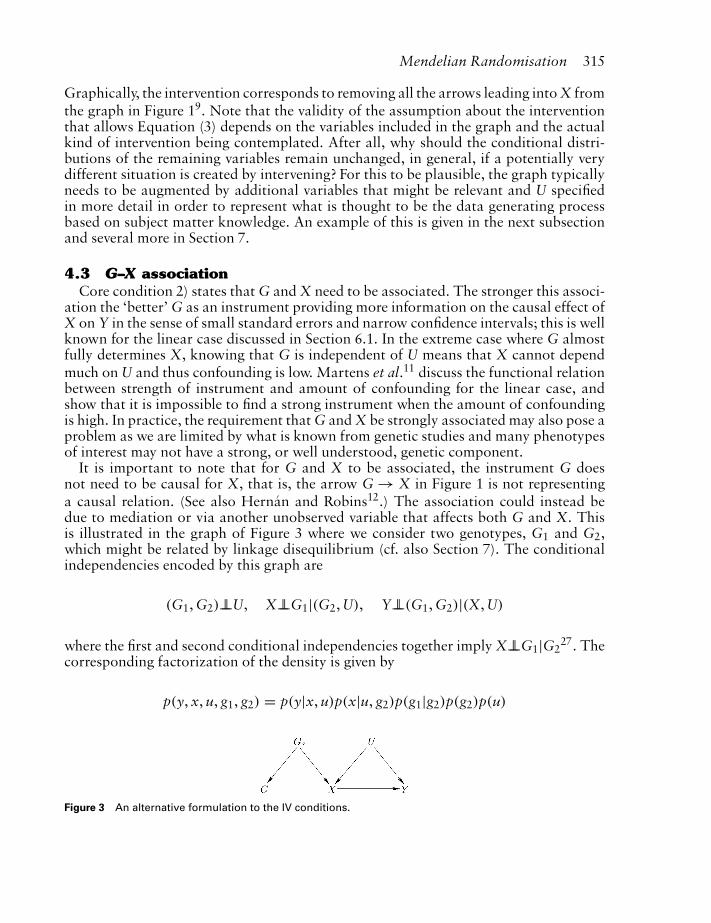
It is important to note that for G and X to be associated, the instrument G doesnot need to be causal for X, that is, the arrow G → X in Figure 1 is not representinga causal relation. (See also Hernán and Robins12.) The association could instead bedue to mediation or via another unobserved variable that affects both G and X. Thisis illustrated in the graph of Figure 3 where we consider two genotypes, G1 and G2,which might be related by linkage disequilibrium (cf. also Section 7). The conditionalindependencies encoded by this graph are
(G1, G2)⊥⊥U, X⊥⊥G1|(G2, U), Y⊥⊥(G1, G2)|(X, U)
where the first and second conditional independencies together imply X⊥⊥G1|G227. The
corresponding factorization of the density is given by
p(y, x, u, g1, g2) = p(y|x, u)p(x|u, g2)p(g1|g2)p(g2)p(u)
Figure 3 An alternative formulation to the IV conditions.

316 V Didelez and N Sheehan
If we believe that we can intervene in X without affecting anything else, we have
p(y, u, g1, g2|do(X = x0)) = p(y|x0, u)p(g1|g2)p(g2)p(u) (4)
Now, assuming that only G1, not G2, is observed, the joint distribution of the remainingvariables is
p(y, x, u, g1) = p(y|x, u)p(x|u, g1)p(g1)p(u)
This is the same as the factorization in Equation (2) and equivalent to assuming our coreconditions 1)–3) with only G1 as IV. It also yields the same intervention distribution asbefore
p(y, u, g1|do(X = x0)) = p(y|x0, u)p(g1)p(u)
which is alternatively obtained by integrating out g2 in Equation (4). For our purposestherefore, we do not have to find the ‘right’ gene as it does not matter how the associationbetween X and the genotype comes about. Hence, without loss of generality, we willassume the situation depicted in Figure 1 and described algebraically in Equation (2),and in Equation (3) for the intervention case. However, as mentioned above, the strongerthe G − X association the better the instrument.
5 Testing for zero causal effect
Assuming that the core conditions 1)–3) of Section 4.1 are satisfied, let us first considerthe situation where we just want to know whether there is a causal link from a phenotypeX to a disease Y without quantifying it. In this section, we investigate whether a testfor dependence between X and Y can be replaced by a test of dependence between theinstrument G and Y. Because of the selection effect in case–control data mentionedabove, we consider prospective and retrospective views separately.
5.1 Prospective viewFrom Equation (3) we obtain the distribution of Y under intervention as
p(y|do(X = x0)) =∑
u,g
p(y|u, x0)p(u)p(g) =∑
u
p(y|u, x0)p(u) (5)
This can be recognized as the usual adjustment formula if U were observable, that is,we partition the population according to U, assess the effect of X on Y within eachsubgroup and then average over the subgroups (Pearl9, p. 78). The ACE, as defined byEquation (1), is then
ACE(x1, x2) =∑
u
(E(Y|U = u, X = x1) − E(Y|U = u, X = x2))p(u)
If E(Y|U = u, X = x) = E(Y|U = u), or more strongly if p(y|u, x) = p(y|u) (i.e.,Y⊥⊥X|U) then the causal effect is obviously zero. Note that Y⊥⊥X|U has a graphical

Mendelian Randomisation 317
Figure 4 DAG representing Y ⊥⊥X | U .
counterpart, shown in Figure 4, which is obtained by deleting the arrow from X to Y inFigure 1. However, the reverse is not necessarily true. If the ACE is zero, or formally ifp(y|do(X = x)) does not depend on x, then we cannot conclude that p(y|u, x) does notdepend on x because, as implied in Equation (5), there could be an interaction betweenX and U in their effect on Y which together with the weights p(u) cancels out the overalleffect. This is the problem of ‘non faithfulness’ – a joint probability distribution is saidto be faithful to a DAG if there are no conditional independence relationships betweenthe variables that do not follow from the directed Markov property.28 In the special caseof models without interactions, more specifically, when for any u �= u′ we have
E(Y|U = u, X = x1) − E(Y|U = u, X = x2)
= E(Y|U = u′, X = x1) − E(Y|U = u′, X = x2)
a zero causal effect leads to the conclusion that E(Y|U, X) does not depend on X. Suchinteractions, of course, can never be completely ruled out as U is unobservable. However,one has to presume that even when allowing for possible interactions between X and U,it would be rare in practice to obtain a zero causal effect without at least having thatE(Y|U = u, X = x) = E(Y|U = u) because the cancellation discussed above requires avery specific numerical configuration.
It would be convenient if (under conditions 1)–3)) Y⊥⊥X|U if and only if Y⊥⊥G. Thiswould imply that if we believed that the conditional distribution of Y under interventionin X is the same as when X is just observed (i.e., the DAG has a causal interpretationso p(y|x, u) = p(y|do(X = x), u)) and if we disregard the particular numerical cancel-lations discussed above, we could test for a causal effect by checking for associationbetween G and Y. Using Equation (2) and integrating out x and u gives the marginaljoint distribution of (Y, G)
p(y, g) = p(g)∑
u
p(u)∑
x
p(y|u, x)p(x|u, g)
We can see that if Y⊥⊥X|U, i.e., if p(y|u, x) = p(y|u), then
p(y, g) = p(g)∑
u
p(y|u)p(u)∑
x
p(x|u, g) = p(g)p(y)
So Y⊥⊥X|U ⇒ Y⊥⊥G. We note that the joint distribution also factorizes if p(x|u, g) =p(x|u), i.e., if X and the IV are not associated but this has been ruled out by corecondition 2).

318 V Didelez and N Sheehan
The reverse argument Y⊥⊥G ⇒ Y⊥⊥X|U does not hold, however, even if we knowthat p(x|u, g) �= p(x|u). Again, this is due to the possibility of very specific numer-ical cancellations that might induce a factorization of p(y, g) without the desiredindependence.
Summarizing, we have
G⊥⊥Y ⇐ Y⊥⊥X | U ⇒ p(y |do(x)) = p(y) (6)
whereas the reverse implications can be violated if specific numerical patterns of theparameters of the involved distributions occur. As the latter would appear unlikely inpractice, we will consider it reasonably safe to regard the three statements in Equation (6)as ‘equivalent for practical purposes’. The complementary implications of Equation (6),especially G⊥⊥/ Y ⇒ Y⊥⊥/ X|U are true in any case, so that if a test finds that G and Y arenot independent we can conclude that the outcome does depend on the phenotype giventhe confounders.
5.2 Retrospective viewIn the case control study situation where we condition on the outcome Y, the data only
allow us to identify properties of the distribution p(x, u, g|y) which from Equation (2)is seen to be
p(x, u, g|y) = p(y|u, x)p(x|u, g)p(u)p(g)∑
x,u p(y|u, x)p(x|u)p(u).
This will typically not factorize in any way: there are no independencies among X, G, Uconditional on Y, as reflected in the moral link induced in the graph by this conditioningand as discussed in Section 4.2. However, assuming, as in the prospective case, that forpractical purposes ‘no causal effect’ is equivalent to Y⊥⊥X|U, then the above conditionaldistribution becomes
p(x, u, g|y) = p(y|u)p(x|u, g)p(u)p(g)∑
u p(y|u)p(u)
if there is no causal effect. By summing out x and u we then find that p(g|y) = p(g).Hence, for a case control study, we can also expect that if there is no causal effect thereshould be no association between Y and G, or equivalently, if we find an associationbetween Y and G then there is a causal effect.
6 Identification of a causal effect
Identifiability of the ACE from observational data requires more than the core conditions1)–3). We consider the additional assumption that all conditional expectations of thevariables in Figure 1 are linear in their graph parents without interactions (Section 6.1).When linearity is doubtful, for instance because the response is binary, it is possible toderive upper and lower bounds for the causal effect (Section 6.2). Section 6.3 addresses

Mendelian Randomisation 319
the question of why the non-linear case cannot be treated in a similar manner to thelinear additive case.
6.1 The easy case: linearity without interactionsIn the following we assume general linear models for the dependencies among the
variables Y, X, G and U. Furthermore, we suppose that all dependencies only affect themean. In other words, we assume that
E(Y|X = x, U = u) = α + β1x + β2u
E(X|G = g, U = u) = γ + δ1g + δ2u (7)
with both X and Y having constant (possibly different) conditional variances. In addi-tion, we assume that the first expectation is the same if we intervene in X, that is, thelink is causal and hence
E(Y|do(X = x0), U = u) = α + β1x0 + β2u
In this framework, as noted in Section 3.2, β1 is the causal parameter that we are inter-ested in since ACE(x1, x2) = β1(x1 − x2). It cannot be estimated from a linear leastsquares regression of Y on X and U, as U is unobserved, nor is it estimable from a linearleast squares regression of Y on X alone, as X and U are correlated. A linear least squaresregression of X on G, however, will yield a consistent estimate rX|G of δ1, the coefficientof G, because G and U are uncorrelated. Since the regression coefficient rY|G of G in alinear least squares regression of Y on G alone can be shown to be consistent for β1δ1,the required causal parameter, β1, can be consistently estimated as the ratio
β̂1 = rY|GrX|G
(see Appendix for technical details.) Obviously we need rX|G to be non-zero but this isprovided by condition 2): G⊥⊥/ X. The variance of β̂1 depends on the conditional varianceof Y given do(X) as well as on the variance of the IV, G, and inversely on the covarianceof X and G (cf. discussion by Martens et al.11). A strong G–X association thus increasesthe precision of the IV estimator, as mentioned in Section 4.3. Note that these resultsrely on models without interactions. In particular, there can be no interactions withthe unobserved confounder U and, since U is unknown, this is obviously an untestableassumption.
Straightforward generalization to the case where G is binary is possible. In this case,the parameter δ1 would then be the mean difference in X for the two different valuesof G. In fact, G can have more than two values as long as its relation with X is linear.The implication for Mendelian randomization applications when G could assume threevalues, one for each genotype in the simplest diallelic case, is that the expected changein X between genotypes 0 and 1 must be the same as the expected change in X betweengenotypes 1 and 2. In other words, the genetic model must be additive. There is nosensible genetic model that is consistent with this requirement for a polymorphic locuswith more than three genotypes.

320 V Didelez and N Sheehan
The case where X is binary is often tackled in the econometrics literature using adummy endogenous variable model.7,29 This is based on a threshold approach whichassumes an underlying unobservable continuous variable Xc with linear conditionalexpectation E(Xc|G, U) as given in Equation (7) above. The observable quantity is Xwhere X = 1 if Xc > 0 and X = 0 otherwise. It can be shown that β1 can still be recoveredas before. (See Appendix for details.)
6.2 Bounds on the causal effectWhen only the core conditions 1)–3) can be assumed without additional assumptions
such as linearity and no interactions, the causal effect is not identifiable and we canat best give lower and upper bounds that will contain the ACE.13−15 This method,however, requires all observable variables to be binary or categorical which could beachieved by suitable categorization of continuous variables. In the binary case, let pij·k =p(Y = i, X = j|G = k) represent the conditional probabilities which can be estimatedeasily from the data using the corresponding relative frequencies. It can be shown thatthe bounds for the average causal effect, ACE(1, 0) = p(Y = 1|do(X = 1)) − p(Y =1|do(X = 0)), are given by
p11.1 + p00.0 − 1p11.0 + p00.1 − 1
p11.0 − p11.1 − p10.1 − p01.0 − p10.0
p11.1 − p11.0 − p10.0 − p01.1 − p10.1
−p01.1 − p10.1
−p01.0 − p10.0
p00.1 − p01.1 − p10.1 − p01.0 − p00.0
p00.0 − p01.0 − p10.0 − p01.1 − p00.1
⎫⎪⎪⎪⎪⎪⎪⎪⎪⎪⎪⎪⎪⎬
⎪⎪⎪⎪⎪⎪⎪⎪⎪⎪⎪⎪⎭
≤ ACE ≤
⎧⎪⎪⎪⎪⎪⎪⎪⎪⎪⎪⎪⎪⎨
⎪⎪⎪⎪⎪⎪⎪⎪⎪⎪⎪⎪⎩
1 − p01.1 − p10.0
1 − p01.0 − p10.1
−p01.0 + p01.1 + p00.1 + p11.0 + p00.0
−p01.1 + p11.1 + p00.1 + p01.0 + p00.0
p11.1 + p00.1
p11.0 + p00.0
−p10.1 + p11.1 + p00.1 + p11.0 + p10.0
−p10.0 + p11.0 + p00.0 + p11.1 + p10.1
These bounds are sharp in the sense that they cannot be improved upon without makingadditional assumptions.15 Wide bounds, possibly containing zero, will reflect that thedata, including the IV, are not very informative for the causal effect. Reasons for thiscould be small sample size, weak instrument or a true ACE close to zero.
In principle, these bounds can also be calculated for factors with more than two levels.However, the more categories there are, the more difficult the computations and the lessinformative the bounds. In Mendelian randomization applications, Y is usually binaryand G can often be considered as binary with one genotype having an effect on the traitand the others pooled into one that has no effect. To calculate the above bounds, wewould dichotomize the usually continuous phenotype X as being above or below a giventhreshold and compare the bounds for different discretizations of X. Note, however, thatthe core conditions then have to be satisfied for the dichotomized version of X, which isnot automatically implied if they hold for the continuous one.
The above bounds are not applicable to the case–control data situation because theyrely on estimating pij.k which cannot be done when the data have been selected on Y.However, knowledge of the disease prevalence, p(y), will almost always be available.

Mendelian Randomisation 321
This, together with the genotype distribution p(g) permits calculation of the bounds forcase–control data since
p(y, x|g) = p(g, x|y)p(y)
p(g)
and p(g, x|y) can be estimated from the data.In practice, the bounds provide an assessment of how informative the data themselves
are in the absence of additional parametric assumptions. Any parametric approachshould therefore be supplemented by the computation of these bounds. Furthermore,by insisting that all the upper bounds are greater than or equal to the lower bounds,testable constraints arise which, if violated, imply that at least one of the core conditionsis not satisfied.
6.3 The difficult caseFrom Section 6.1 and the corresponding derivations in the Appendix we can see that
in order to use the IV technique we need to, firstly, specify what our causal parameter isand, secondly, determine how it relates to the regression parameters of a regression of Xon G and a regression of Y on G. The latter involves marginalizing over U and the resultin the non-linear case is typically not independent of the unknown distribution of U.
6.3.1 Causal parameter for non-linear modelsAssume we have a binary response variable Y, as is the case in many epidemiological
applications. The ACE is then the risk difference. To determine the ACE, we have tointegrate out U in order to determine E(Y|do(X = x)), which in the case of a non-lineardependence of Y on X and U will typically depend on the unknown distribution of U.For instance, assuming a logistic regression we obtain
E(Y|do(X = x)) =∫
exp{α + β1x + β2u}1 + exp{α + β1x + β2u}p(u) du (8)
where p(u) is the unknown density of U. The above expectation cannot generally bewritten in the same model form with a different constant. In particular, for this case,
E(Y|do(X = x)) �= exp{α∗ + β1x}1 + exp{α∗ + β1x} (9)
even when U is assumed to be normally distributed. Greenland et al.30 discuss thisproblem referring to it as non-collapsibility of the logistic regression model.
Alternative causal parameters are the odds ratio or relative risk. The former is par-ticularly important when the data come from case–control studies, as these only allowidentification of odds ratios. We can define the causal odds ratio (COR) as
COR(x1, x2) = p(Y = 1|do(X = x1))
p(Y = 0|do(X = x1))
p(Y = 0|do(X = x2))
p(Y = 1|do(X = x2))

322 V Didelez and N Sheehan
where p(Y = 1|do(X = x1)) = E(Y|do(X = x1)). However, from Equations (8) and (9),it is not guaranteed that β1 is the causal parameter of interest in the sense that
COR(x1, x2) �= exp{β1(x1 − x2)}In fact, COR again depends on the unknown confounder distribution. For the causal
relative risk (CRR) defined as
CRR(x1, x2) = p(Y = 1|do(X = x1))
p(Y = 1|do(X = x2))
we consider a (causal) log-linear model corresponding to this parameter
E(Y|X = x, U = u) = E(Y|do(X = x), U = u) = exp{α + β1x + β2u}which does imply that E(Y|do(X = x)) = exp{α∗ + β1x} after marginalizing over U(where typically α∗ �= α), independently of the distribution of U. Thus, the log-linearshape is retained, CRR is exp{β1(x1 − x2)} and β1 is the relevant causal parameter.
6.3.2 Relationship between regression parametersThe next step is to investigate how the regression parameters estimated by a regression
of Y on G and a regression of X on G are related to the causal parameter of interest.From the Appendix we see that this relies on working out
E(Y|G = g) = EUEX|U,G=gE(Y|X, U)
that is, we compute the conditional expectation of Y given (X, U), then integrate out Xwith regard to its conditional distribution given (U, G = g) and then integrate out U withrespect to its marginal distribution, thus exploiting the core conditional independenciesto obtain the conditional expectation of Y given G. The derivation in the Appendix cru-cially depends on the different expectations being additive in the conditioning variablesso that taking expectations is straightforward. But if we assume a logistic regressionfor a binary response variable Y, E(Y|X, U) = p(Y = 1|X, U) is not additive in X andU and so the expectation EX|U,G=gE(Y|X, U) is not straightforward to compute as itinvolves an integral to which there is not necessarily an analytic solution. Thompsonet al.31 suggest an approximation. However, this approximation ignores U and assumesthat Y ⊥⊥ G|X which, if true, would mean that an IV approach is unnecessary as therewould be no confounding and the effect of X on Y could be estimated from the data.Hence, this does not provide a way of identifying the COR in the situation where thereis confounding but it can be used as a heuristic check for the presence of confounding.32
If we model p(Y = 1|X, U) log-linearly corresponding to the CRR, then E(Y|X, U) =p(Y = 1|X, U) is multiplicative in X and U and is again not additive. Hence, justas for the logistic relationship, solving E(Y|G = g) = EUEX|U,G=gE(Y|X, U) requiresan approximation. The derivation provided in Thomas and Conti33 also ignores Uand assumes that Y ⊥⊥ G|X. The same general problem arises with the approxima-tion for the probit link that these authors refer to. The probit model can however be

Mendelian Randomisation 323
used under certain assumptions when it is held that all binary variables are generatedby unobserved underlying continuous variables that have a joint multivariate normaldistribution.34
7 Complications for Mendelian randomization
The limitations of Mendelian randomization, from the perspective of complicat-ing features leading to poor estimation of the required genotype–phenotype andgenotype–disease associations, have been discussed in detail in several places in theliterature.5,33,35,36 More crucially, biological complications can sometimes violate oneor more of the core conditions 1)–3) so that Figure 1 no longer applies. Our focushere is on explicating what any added complexity implies with regard to meet-ing these conditions. This is illustrated using DAGs that are ideally dictated by thebiology.
Linkage disequilibrium refers to the association between alleles at different loci acrossthe population, as is the case when loci are physically close on the chromosome andthus tend to be inherited together, or may be due to other reasons such as naturalselection, assortative mating and migration.37 When our chosen gene G1 is in linkagedisequilibrium with another gene G2 which has a direct or indirect influence on thedisease Y, condition 3) (Y ⊥⊥ G1|(X, U)) might be violated, as shown in Figure 5(a), orelse condition 1) (G ⊥⊥ U) might be violated, as shown in Figure 5(b).
Pleiotropy is the phenomenon whereby a single gene may influence several traits. If thechosen instrument G is associated with another intermediate phenotype which also hasan effect on the disease Y (Figure 6(a)), condition 3), Y ⊥⊥ G|(X1, U), is again violated ifwe do not also condition on X2. Moreover, a genetic polymorphism under study mighthave pleiotropic effects that influence confounding factors like consumption of tobaccoor alcohol, for example, Davey Smith and Ebrahim5. This is represented in Figure 6(b)and violates condition 1).
Figure 5 Linkage disequilibrium in a Mendelian randomization application.
Figure 6 Pleiotropy in a Mendelian randomization application.

324 V Didelez and N Sheehan
Genetic heterogeneity arises when more than one gene affects the phenotype. Thecore conditions may still hold for the chosen instrument G1 in the situation of Figure 7,where none of the other genes influence Y in any way other than via their effect on X. Ifinstead the situation is similar to Figure 5(b), for example, the core conditions may beviolated as already explained. Also, in Figure 7, genetic heterogeneity could weaken theG1–X association.
Population stratification denotes the co-existence of different disease rates and allelefrequencies within subgroups of individuals. In Figure 8(a), we see that condition 3), Y ⊥⊥G1|(X, U), is again violated: we need to condition on the population subgroup as well.However, if population stratification causes an association between allele frequenciesand phenotype levels, as in Figure 8(b), all conditions for G to be an instrument arestill satisfied, and, in this situation, the G–X association may in fact be strengthened orweakened, as a result.
Furthermore, the true biological situation could involve several genes affecting severalphenotypes whose joint influence on the disease of interest is subject to confounding (Fig-ure 9). Keavney et al.38 consider six lipid-related genes and two plasma apolipoproteinsaffecting CHD. Each gene was considered as a separate instrument and the ratio of theplasma lipoproteins taken as the intermediate phenotype. However, the reported geno-type–CHD associations were not consistent with the genotype–phenotype associationswhereby genes that adversely affected lipoprotein levels were not necessarily associatedwith increased risk of CHD. One explanation is that the underlying biology is more likeFigure 9 and that interactions between genes and between phenotypes need to be taken
Figure 7 Genetic heterogeneity in a Mendelian randomization application.
Figure 8 Two examples of population stratification for Mendelian randomization.
Figure 9 A more complicated example for gene–phenotype–disease relations.

Mendelian Randomisation 325
into account. There is currently no simple extension of the current IV approach that isapplicable to this situation.
8 Discussion
It seems to us that applications of Mendelian randomization can benefit from a for-mal framework for causal inference.39 For example, the ‘do’ operation of Pearl9 thatwe have used in the present paper allows explicit specification of what the causal aimunder investigation is and under which conditions it can be attained. We argue andconfirm that Mendelian randomization can often be reasonably assumed to satisfy theconditions of an IV. Moreover, these core conditions can be represented using DAGsand can hence be verified by visual inspection (e.g., Section 7). Our focus regardingcausal inference is on testing for and estimating the causal effect, and on the specialcase of retrospective as opposed to prospective studies. Our findings are as follows.Testing for a phenotype–disease causal effect by testing for a genotype–disease asso-ciation, as suggested by Katan16, is reasonable for practical purposes (Section 5). Forcalculation of the ACE, one must rely on additional strong parametric assumptionssuch as linearity and no interactions but these are not typically justifiable for epidemi-ological applications with a binary disease outcome. At least, one should carry outsensitivity analyses if such models are used. In the non-linear/interaction case, even thespecification of the causal parameter is not obvious and determination of its relation-ship to the relevant regression parameters is not straightforward (Section 6). ‘There is,in fact, no agreed upon generalization of IVs to non-linear systems’9. This is partic-ularly alarming as in a case–control study, generally only the odds ratio can sensiblybe considered. Assuming no more than the core conditions for a genotype to be aninstrument, bounds on the ACE can always be calculated if all variables are binaryand these can be adapted to the case–control situation if the disease prevalence isknown.
The above framework leads us to see the limitations of Mendelian randomization asfalling into two main categories: in some situations, the core assumptions for a genotypeto be an instrument are not plausible (Section 7), and in other cases, the parametricassumptions that are required to calculate the causal effect are not reasonable. Whilethere is much discussion in the literature about the difficulty of obtaining good estimatesfrom genetic association studies, in particular, due to lack of power or because theestimates come from different studies,17 the current approaches to testing and estimatingthe relevant causal effects are rarely challenged. For instance, the ratio point estimate forthe relevant regression parameter which is valid in the additive linear case (Section 6.1)has been advocated as appropriate for binary outcomes,33,40 which seems dubious to us.Even in a recent article,41 while it is noted that linearity is required for this estimate, theassertion that such assumptions are ‘not easily satisfied in a Mendelian randomizationsetting’ is not discussed.
In summary, we regard the following issues as most important and pressing for furtherresearch in order to widen the applicability of the method of Mendelian randomization:

326 V Didelez and N Sheehan
general methods for the non-linear case and consideration of different causal parameters.The econometric literature could be a promising source of IV methods for some non-linear models.42,43 In particular, proposals for estimation of the CRR (cf. Mullahy44
or Windmeijer and Santos Silva45) have to be scrutinized with regard to the requiredassumptions and might be combined with logit models when events are rare.46 A draw-back of these methods is that interactions between the phenotype and the confoundingfactors are excluded which is a restrictive assumption and calls for generalizations as wellas thorough sensitivity analyses. Also, advances made in connection with the so-calledlocal causal effect based on randomized trials with partial compliance need to be scruti-nized as to whether this causal parameter is meaningful in a Mendelian randomizationsetting and whether it may be estimated in situations where the ACE cannot. A generalmodel class proposed in this context is the one of structural mean models (cf. overviewin Hernán and Robins12). Bayesian approaches have also been proposed for this RCTscenario.47 These, again, require further investigation.
Appendix
Background on the linear and no interactions caseLet us first show why β1 is the causal parameter of interest. With the assumptions
from Section 6.1, we have that
E(Y|do(X = x)) = EU|do(X=x)E(Y|do(X = x), U)
= EUE(Y|do(X = x), U)
= α + β1x + β2μU
= α∗ + β1x
where μU = E(U) and using obvious notation for iterated conditional expectation. Thesecond equality holds because do(X = x) is not informative for U as there cannot be anydependence between an intervention and an unknown variable (graphically, interveningon X removes the arrows leading into X from Figure 1). From the above, we obtain
ACE(x1, x2) = β1(x1 − x2)
so we are interested in estimating β1.Using the usual conditioning without intervention, a regression of Y on X alone
corresponds to
E(Y|X = x) = EU|X=xE(Y|X = x, U)
= α + β1x + β2μU|X=x
where μU|X=x = E(U|X = x) is typically not constant in x, in particular not equal toμU, due to the dependence between X and U in the non-interventional case, that is, in

Mendelian Randomisation 327
the observational regime. Hence β1 cannot be identified from a regression of Y on Xalone.
Instead consider a regression of Y on G alone. This corresponds to
E(Y|G = g) = E(X,U)|G=gE(Y|X, U, G = g)
= EU|G=gEX|U,G=gE(Y|X, U) since Y ⊥⊥ G|(X, U)
= EUEX|U,G=gE(Y|X, U) since U ⊥⊥ G
= EU(α + β1(γ + δ1g + δ2U) + β2U)
= α + β1γ + β1δ1g + (β1δ2 + β2)μU
= α∗ + β1δ1g
Hence, the coefficient of G in a regression of Y on G is β1δ1.Furthermore, a regression of X on G alone corresponds to
E(X|G = g) = EU|G=gE(X|G = g, U)
= EUE(X|G = g, U)
= γ + δ1g + δ2μU
so the coefficient of G in this regression is δ1. Thus, as given in Section 6.1, the causalparameter of interest, β1, can be estimated from the ratio of these two regression coef-ficients. This is usually done in a ‘two-stage-least-squares’ procedure: more details canbe found in Stewart and Gill48.
Threshold modelsThe above can be generalized to the case of binary G and X in the following way. Let
E(Y|X = x, U = u) = α + β1x + β2u, as before. Consider an underlying unobservedvariable Xc with
E(Xc|G = g, U = u) = γ + δ1g + δ2u
and define
X ={
1, Xc > 0
0, otherwise
The dependence structure can be represented as in Figure 10 where the relationshipbetween Xc and X is deterministic. The conditional independencies with respect to allvariables are Y ⊥⊥ (G, Xc)|(U, X), X ⊥⊥ (G, U)|Xc and G ⊥⊥ U. But as Xc is not observedwe have Y ⊥⊥ G|(U, X), X ⊥⊥� G and still G ⊥⊥ U for the remaining variables. Hence, thecore conditions 1)–3) apply to (G, U, X, Y), ignoring Xc, and β1 is still the parameterwe are interested in as it describes the required causal effect.
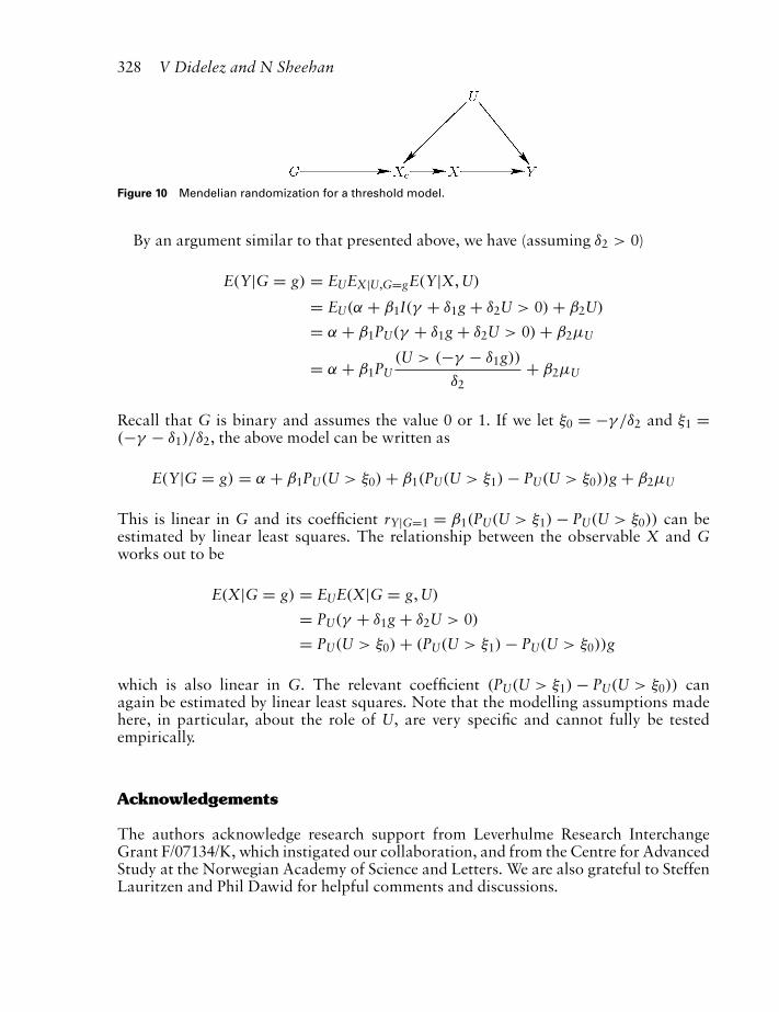
328 V Didelez and N Sheehan
Figure 10 Mendelian randomization for a threshold model.
By an argument similar to that presented above, we have (assuming δ2 > 0)
E(Y|G = g) = EUEX|U,G=gE(Y|X, U)
= EU(α + β1I(γ + δ1g + δ2U > 0) + β2U)
= α + β1PU(γ + δ1g + δ2U > 0) + β2μU
= α + β1PU(U > (−γ − δ1g))
δ2+ β2μU
Recall that G is binary and assumes the value 0 or 1. If we let ξ0 = −γ /δ2 and ξ1 =(−γ − δ1)/δ2, the above model can be written as
E(Y|G = g) = α + β1PU(U > ξ0) + β1(PU(U > ξ1) − PU(U > ξ0))g + β2μU
This is linear in G and its coefficient rY|G=1 = β1(PU(U > ξ1) − PU(U > ξ0)) can beestimated by linear least squares. The relationship between the observable X and Gworks out to be
E(X|G = g) = EUE(X|G = g, U)
= PU(γ + δ1g + δ2U > 0)
= PU(U > ξ0) + (PU(U > ξ1) − PU(U > ξ0))g
which is also linear in G. The relevant coefficient (PU(U > ξ1) − PU(U > ξ0)) canagain be estimated by linear least squares. Note that the modelling assumptions madehere, in particular, about the role of U, are very specific and cannot fully be testedempirically.
Acknowledgements
The authors acknowledge research support from Leverhulme Research InterchangeGrant F/07134/K, which instigated our collaboration, and from the Centre for AdvancedStudy at the Norwegian Academy of Science and Letters. We are also grateful to SteffenLauritzen and Phil Dawid for helpful comments and discussions.

Mendelian Randomisation 329
References
1 Fisher RA. The design of experiments, firstedition. Oliver & Boyd, 1926.
2 Fisher RA. The design of experiments, eigthedition. Hafner, 1970.
3 Peto R, Doll R, Buckley JD, Sporn MB. Candietary beta-carotene materially reducehuman cancer rates? Nature 1981; 290: 201–8.
4 Alpha-Tocopherol, Beta Carotene CancerPrevention Study Group. The effect ofvitamin E and beta carotene on the incidenceof lung cancer and other cancers in malesmokers. New England Journal of Medicine1994; 330: 1029–35.
5 Davey Smith G, Ebrahim S. Mendelianrandomization: can genetic epidemiologycontribute to understanding environmentaldeterminants of disease? InternationalJournal of Epidemiology 2003; 32: 1–22.
6 Katan MB. Commentary: Mendelianrandomization, 18 years on. InternationalJournal of Epidemiology 2004; 33: 10–11.
7 Bowden RJ, Turkington DA. Instrumentalvariables. Cambridge University Press, 1984.
8 Angrist JD, Imbens GW, Rubin DB.Identification of causal effects usinginstrumental variables. Journal of theAmerican Statistical Association 1996;91(434):444–55.
9 Pearl J. Causality (Chapter 7). CambridgeUniversity Press, 2000.
10 Greenland S. An introduction to instrumentalvariables for epidemiologists. InternationalJournal of Epidemiology 2000; 29:722–9.
11 Martens EP, Pestman WR, de Boer A, BelitserSV, Klungel OH. Instrumental variables,application and limitations. Epidemiology2006; 17: 260–7.
12 Hernán MA, Robins JM. Instruments forcausal inference. An epidemiologist’s dream?Epidemiology 2006; 17: 360–2.
13 Robins JM. The analysis of randomized andnonrandomized aids treatment trials using anew approach to causal inference inlongitudinal studies. In L, Sechrest H,Freeman and A. Mulley eds. Health ServiceResearch Methodology. A Focus on AIDS.U.S. Public Health Service, 1989: 113–59.
14 Manski CF. Nonparametric bounds ontreatment effects. American EconomicReview, Papers and Proceedings 1990; 80:319–23.
15 Balke AA, Pearl J. Counterfactualprobabilities: computational methods,
bounds and applications. In Mantaras RL,Poole D. eds. Proceedings of the 10thConference on Uncertainty in ArtificialInteligence. 1994: 46–54.
16 Katan MB. Apolipoprotein E isoforms, serumcholesterol, and cancer. Lancet 1986; i:507–8.
17 Minelli C, Thompson JR, Tobin MD,Abrams KR. An integrated approach to theMeta-Analysis of genetic association studiesusing Mendelian randomization. AmericanJournal of Epidemiology 2004; 160:445–52.
18 Scandinavian Simvastin Survival Study (4S).Randomised trial of cholesterol lowering in4444 patients with coronary heart disease.Lancet 1994; 344: 1383–9.
19 Heart Protection Study Collaborative Group.MRC/BHF heart protection study ofcholesterol lowering with simvastin in 20,536high-risk individuals. Lancet 2002; 360:7–22.
20 Pearl J. Causal diagrams for empiricalresearch. Biometrika 1995; 82: 669–710.
21 Lauritzen SL. Causal inference fromgraphical models. In Barndorff-Nielsen OE,Cox DR, Kluppelberg C. eds. ComplexStochastic Systems. Chapter 2, Chapman &Hall, 2000: 63–107.
22 Dawid AP. Influence diagrams for causalmodelling and inference. InternationalStatistical Review 2002; 70: 161–89.
23 Dawid AP. Causal inference using influencediagrams: the problem of partial compliance.In Green PJ, Hjort NL, Richardson S. eds.Highly Structured Stochastic Systems.Oxford University Press, 2003: 45–81.
24 Goldberger AS. Structural equation methodsin the social sciences. Econometrica 1972; 40:979–1001.
25 Pearl J. Probabilistic reasoning in intelligentsystems. Morgan Kaufmann, 1988.
26 Cowell RG, Dawid AP, Lauritzen SL,Spiegelhalter DJ. Probabilistic networks andexpert systems. Statistics for Engineering andInformation Science, Springer-Verlag, 1999.
27 Dawid AP. Conditional independence instatistical theory (with Discussion). Journalof the Royal Statistical Society, Series B 1979;41: 1–31.
28 Spirtes P, Glymour C, Scheines R. Causation,prediction and search, second edition. MITPress, 2000.

330 V Didelez and N Sheehan
29 Maddala GS. Limited-dependent andqualitative variables in econometrics.Cambridge University Press, 1983.
30 Greenland S, Robins JM, Pearl J.Confounding and collapsibility in causalinference. Statistical Science 1999; 14: 29–46.
31 Thompson JR, Tobin MD, Minelli C. On theaccuracy of the effect of phenotype on diseasederived from Mendelian randomisationstudies. Genetic Epidemiology TechnicalReport 2003/GE1, Centre for Biostatistics,Department of Health Sciences, University ofLeicester, 2003. Retrieved fromhttp://www.prw.le.ac.uk/research/HCG/getechrep.html.
32 Didelez V, Sheehan NA. Mendelianrandomisation and instrumental variables:what can and what can’t be done. TechnicalReport 05-02, Department of Health Sciences,University of Leicester, 2005. Retrieved fromhttp://www.homepages.ucl.ac.uk/ucakvdi/vlon.html.
33 Thomas DC, Conti DV. Commentary: theconcept of ‘Mendelian randomization’.International Journal of Epidemiology 2004;33: 21–5.
34 Stanghellini E, Wermuth N. On identificationof path analysis models with one hiddenvariable. Biometrika 2005; 92: 337–50.
35 Davey Smith G, Ebrahim S. Mendelianrandomization: prospects, potentials, andlimitations. International Journal ofEpidemiology 2004; 33: 30–42.
36 Davey Smith G, Ebrahim S, Lewis S, HansellAL, Palmer LJ, Burton PR. Geneticepidemiology and public health: hope, hype,and future prospects. Lancet 2005a; 366:1484–98.
37 Lynch M, Walsh B. Genetics and analysis ofquantitative traits. Sinauer Associates Inc.,1998.
38 Keavney BD, Palmer A, Parish S, Clark S,Youngman LD, Danesh J, McKenzie C,Delphine M, Lathrop M, Peto R, Collins R.Lipid-related genes and myocardial infarcionin 4685 cases and 3460 controls: discrepanciesbetween genotype, blood lipidconcentrations, and coronary disease risk.International Journal of Epidemiology 2004;33: 1002–13.
39 Didelez V, Sheehan NA. Mendelianrandomisation: why epidemiology needs aformal language for causality. In Russo F, andWilliamson J, ed. Causality and Probability inthe Sciences. London College Publications,Texts in philosophy 2007; 5: 263–292.
40 Davey Smith G, Lawlor DA, Harbord R,Timpson N, Rumley A, Lowe GDO, DayINM, Ebrahim S. Association of C-reactiveprotein with blood pressure andhypertension: life course confounding andMendelian randomisation tests of causality.Arteriosclerosis, Thrombosis and VascularBiology 2005b; 25: 1051–56.
41 Nitsch D, Molokhia M, Smeeth L, DeStavolaBL, Whittaker JC, Leon DA. Limits to causalinference based on Mendelianrandomization: a comparison withrandomised controlled trials. AmericanJournal of Epidemiology 2006; 163:397–403.
42 Amemiya T. The nonlinear two-stageleast-squares estimator. Journal ofEconometrics 1974; 2: 105–10.
43 Hansen LP, Singleton RJ. Generalizedinstrumental variable estimation ofnon-linear rational expectation models.Econometrica 1982; 50: 1269–86.
44 Mullahy J. Instrumental variable estimationof Poisson regression models: application tomodels of cigarette smoking behaviour.Review of Economics and Statistics 1997; 79:586–93.
45 Windmeijer F, Santos Silva JMC. Endogeneityin count data models: an application todemand for health care. Journal of AppliedEconometrics 1997; 12: 281–94.
46 Rosner B, Spiegelman D, Willett WC.Correction of logistic regression relative riskestimates and confidence intervals formeasurement error: the case of multiplecovariates measured with error. AmericanJournal of Epidemiology 1990; 132:734–45.
47 Imbens GW, Rubin DB. Bayesian inference forcausal effects in randomized experimentswith noncompliance. The Annals of Statistics1997; 25: 305–27.
48 Stewart J, Gill L. Econometrics, secondedition. Prentice & Hall, 1998.