Memory Analysis of Solid Model Representations for ...

Memory Analysis of Solid Model Representations

for Heterogeneous Objects

T. R. Jackson1, W. Cho2, N. M. Patrikalakis2, E. M. Sachs2

([email protected], [email protected], [email protected], [email protected])

1The Charles Stark Draper Laboratory, 2Massachusetts Institute of Technology

Abstract

Methods to represent and exchange parts consisting of Functionally Graded Material

(FGM) for Solid Freeform Fabrication (SFF) with Local Composition Control (LCC)

are evaluated based on their memory requirements. Data structures for representing

FGM objects as heterogeneous models are described and analyzed, including a

voxel-based structure, finite-element mesh-based approach, and the extension of the

Radial-Edge and Cell-Tuple-Graph data structures with Material Domains

representing spatially varying composition properties. The storage cost for each data

structure is derived in terms of the number of instances of each of its fundamental

classes required to represent an FGM object. In order to determine the optimal data

structure, the storage cost associated with each data structure is calculated for

several hypothetical models. Limitations of these representation schemes are

discussed and directions for future research also recommended.

Keywords: Solid Freeform Fabrication (SFF); Local Composition Control (LCC); Functionally Graded Materials (FGM);

heterogeneous objects; storage cost analysis; data structures for heterogeneous objects.

Introduction

With recent advances in Solid Freeform Fabrication (SFF), the ability to fabricate parts with Local

Composition Control (LCC)1 is becoming a reality, opening the door to creating a whole new class of

components [1,2,3,4,5,10,11,12,13,18,20]. Material composition can be tailored within a component to

achieve local control of properties (e.g., index of refraction, electrical conductivity, formability, magnetic

properties, corrosion resistance, hardness vs. toughness, etc.). Such compositions have become known as

Functionally Graded Material (FGM). By such local control, monolithic components can be created which

integrate the function of multiple discrete components, saving part count, space and weight and enabling

concepts that would be otherwise impractical. Controlling the spatial distribution of properties via

composition will allow for control of the state of the entire component (e.g., the state of residual stress in a

component). Fabrication of integrated sensors and actuators can be envisioned with LCC (e.g., bimetallic

structures, in-situ thermocouples, etc.). Even devices designed to control chemical reactions would be

possible.

Despite the advanced capabilities of SFF, access to this new technology is limited by how information is

represented, exchanged, and processed. Designers need new CAD representations to capture their ideas

as FGM models and manufacturers need algorithms capable of converting these models into machine

instructions for their fabrication. A method for maintaining this information, however, has not yet been

adopted as the preferred solution from the many approaches to representing volumetric data. This presents

an obstacle to the exploration of tools for capturing design intent, algorithms for processing models for

fabrication, and finally exercising the capabilities of LCC, as each method maintains data differently and

follows a different paradigm. One of the major obstacles to choosing a solid modeling method through

which to explore modeling objects with LCC is the memory required to accurately store information within

the model. By investigating the memory requirements for various approaches to representing parts with

In this paper, the following definitions apply: SFF is any additive manufacturing process, LCC is the capability tocontrol composition during fabrication, a heterogeneous object is any object composed of multiple materials, and anFGM is a material whose properties vary smoothly over a space, designed for a specific function.1

LCC, a decision about which method should be preferred as the basis for the solid modeling for

heterogeneous objects can be made [1].

Volumetric data is often represented in voxel- or mesh-based structures for analysis purposes. The use of

voxel-based or exhaustive enumeration methods is common for volumetric data sampled from the real-

world. The structure of a voxelized model consists of cells uniformly distributed over a 3D grid. Each cell

maintains information about its composition. Kaufman et al. [6] provided a summary of the advantages and

disadvantages of voxel-based modeling methods: insensitivity to the scene complexity, high storage costs

and loss of geometric information about specific surfaces and features as a result of discretization. Citing

the close resemblance between how voxel-based methods represent parts and how SFF processes build

parts, researchers have suggested the use of such methods for SFF model representation and design [7].

Chandru et al. [8] suggested that process planning for SFF fabrication is greatly simplified through the use of

a voxel representation. They also suggested the possibility of building composite structures by associating

material information with each voxel, thereby enabling the representation/design of parts for LCC. To

address high storage costs, they suggested trading computation time with memory cost by compression,

octrees, shells, or maintain the original geometric representation and use voxelization algorithms when

necessary. In CAD, designs and physical problems are often analyzed through the finite-element method,

allowing the study and prediction of engineering properties, in which CAD models are decomposed into

meshes of elements with interpolating functions. With its ability to represent volumetric data, the finite-

element modeling is another avenue for establishing a representation and design of FGM objects , as

proposed by Pegna and Safi [9]. They suggested that models represented by point sets used in existing

finite-element analysis systems could readily be used to model FGM parts.

Another source of inspiration for modeling volumetric material information is texturing algorithms used in

computer graphics. Similar to how clouds and smoke can be rendered in a virtual reality environment, Park

et al. [10] have developed a Volumetric Multi-Texturing (VMT) method for representing FGM objects based

on procedural algorithms for evaluating material variation within a model. Their method attaches volumetric,

material blending functions, in a procedural way, to entities in an existing solid modeling engine. During

evaluation, the functions are evaluated in procedural manner to determine the composition at a point.

While the preceding approaches to FGM modeling adopt analysis or graphics rendering methods for

volumetric data to the representation and design of FGM objects, another avenue to solving this problem is

to extend solid modeling methods currently used in CAD systems to handle graded material data. Kumar et

al. [11,12,13] have proposed the extension of solid modeling to handle heterogeneous objects by using r-

sets with information about material variation (rm-sets). The shape of a model is defined in terms of an r-set

(a form of B-rep modeling). This geometry model is further decomposed into atlases over which material

variations are mapped. In such a manner, FGM solid models are represented as rm -objects, maintaining the

geometry of the model’s boundary and the volume fraction variation of each material throughout the object.

A generalized cellular decomposition approach to FGM solid modeling was identified by Bardis and

Patrikalakis [14], in the early 90’s, and developed further by the authors of this paper [4,5] where a solid

model is decomposed into a collection of cells representing the vertices, edges, faces, and regions of the

solid model. The topology (or connectivity between the cells) is maintained through the use of a data

structure known as the Cell-Tuple data structure [15,16]. The geometry of each cell is maintained

separately, similar to how the geometry is maintained in the existing B-rep modelers. Along with the

geometry of each cell, material information is also stored, allowing modeling of both curved geometries and

graded compositions for each cell. Upon close review, it becomes apparent that the above two approaches

advocate decomposition of models into general regions over which material variations are mapped.

This paper is structured as follows. First, the issues involved in modeling FGM objects for LCC fabrication

are identified, including the goal and how their modeling fits into the overall information flow. Next,

candidate data structures are presented in terms of class associations and expressions for the memory

required for each are formed based on the number of instances of each class. An example part is then

discussed, demonstrating how the storage costs for a hypothetical model can be predicted. Finally, we

conclude with observations about modeling methods for heterogeneous objects and recommendations for

future research.

Identification of FGM Modeling Issues

In simplest terms, the goal of a data structure for CAD is to represent a part or object (real or proposed)

accurately in the digital domain for the purposes of design, analysis, and fabrication. In the majority of CAD

applications, parts consisting of single materials can be modeled by accurately describing the boundary of

the parts’ interiors (their geometric features and shape). For objects to be fabricated with LCC, however,

additional requirements are imposed. The ability to vary the composition of the interior requires that the

underlying data structure not only represents boundaries accurately, but variations in composition as well.

This section presents the issues involved in modeling FGM parts, identifying the Model Space required for

representing FGM objects. An overall flow for this information from design to fabrication is then described,

clearly separating issues in design and modeling from SFF fabrication.

Geometric and material modeling

Modeling the geometry (or shape) of an object is the primary purpose of most design systems. Existing

CAD systems provide this functionality with the capability to model a single part of a single material or an

assembly, consisting of several models. The Model Space maintained in these data structures can be

considered a Build Space in R3 in which the model will be fabricated (see Figure 1). The stored boundary of

the model must clearly divide this Build Space into the interior and exterior of the model. To accomplish this,

any of a number of solid modeling methods may be used (voxel-based, CSG, B-rep, cellular decomposition,

etc). The designer modifies the boundary of the object through a set of design tools (extrude, cut, sweep,

revolve, etc.) to generate the desired shape. In addition to representing the object, queries about the

geometric nature of the boundary may be made. These geometric interrogations may consist of calculating

quantities such as surface normals, curvature, minimum distance between features, surface area, or

volume. In the current geometric modeling systems, although material information may be associated with a

geometric model, it can be considered as an attribute attached to the enclosed region and is assumed to be

uniform throughout that region.

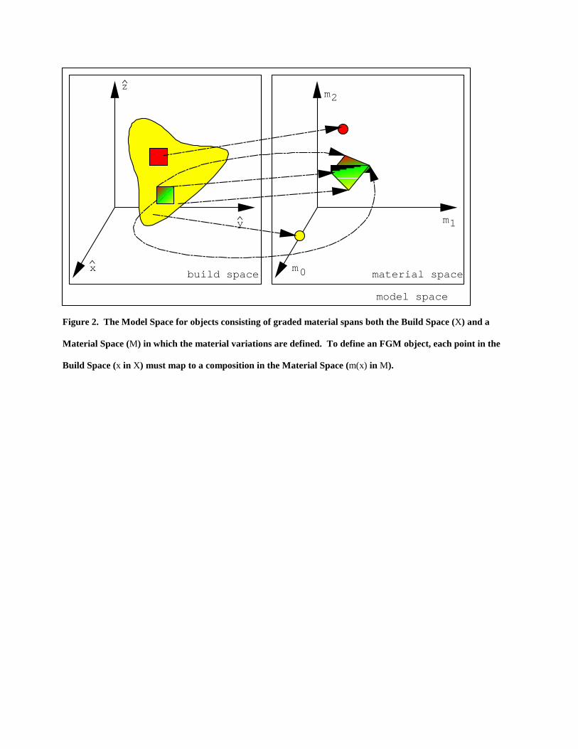
With the goal of modeling graded compositions, the issue of material modeling becomes as important to the

definition of a data structure as the geometric modeling of boundaries. For such applications, the Model

Space should be considered as a combination of the Build Space and a Material Space, defining the models

geometry and composition, respectively (see Figure 2). As before, the Build Space is the three-dimensional

space in which the object is to be fabricated. The Material Space, however, is spanned by the primary

materials in the material system. This concept is analogous to the blending of primary colors (Cyan, Yellow,

Magenta, and Black) in an ink-jet printer to produce a wide range of colors and tones for color hard-copy

output. To achieve LCC, an SFF process builds a part by selectively adding varying quantities of different

base materials. These materials comprising the material system create a Material Space out of which an

FGM is defined. The dimension of the Material Space (dm) is the number of materials out of which the object

is to be composed. To define an FGM object, a mapping from the Build Space (X) into the Material Space

(M) must be provided. This concept has previously been suggested by Kumar et al. [11,12] (through the

use of atlases) and Jackson et al. [4,5,1] (through the use of parametric cells with control points in Build

Space and control compositions in Material Space). This concept of mapping from Build Space into Material

Space is illustrated in Figure 2. Therefore, for FGM modeling, the goal is to define a function spanning the

material space for all the points in Build Space, uniquely and accurately defining models’ composition.

To assist in the definition of the underlying data structure, the concept of composition (m(x)) is introduced,

defining the volume fraction of each of the primary materials at every point in the Build Space.

For completeness, the material “voids” are always included to allow the definition of space exterior to the

object’s intended boundary. In addition, further restrictions are imposed on the composition function such

that the volume fractions always sum to unity and the volume fraction of each material is non-negative:

10for 0.0 and01 )( 1101−≤≤≥=+++= − mid dim.mmm

m�xm

=

=

−− 1

1

0

1

1

0

%

%

%

)(

mm dd m

m

m

material

material

material

��xm

Tools for working with geometric information (the object’s boundary) are still important, but how the material

varies throughout the model is now equally important at the time of design. The composition may vary

smoothly or contain discontinuities, depending on what tools are used for defining m(x), how this information

is modeled, and the designer’s intent. In essence, the goal of a method for defining FGM models is simply

to represent m(x) as accurately and efficiently as possible.

Accuracy in model representation

The quality of the digital representation of a designer’s intent can be quantified in terms of accuracy. For

FGM models, the accuracy in representation involves two parts: geometric (shape) and material

(composition). Geometric accuracy describes how accurately the digital description of the part matches the

designer’s intended shape. For the purposes of this paper, geometric accuracy is defined as the maximum

deviation between the desired shape and the shape stored digitally (see Figure 3). With the representation

of graded material information, the concept of material accuracy must also be defined. Material accuracy is

the maximum difference between the intended volume fraction for any material at any point in the object and

the volume fraction actually maintained or computed from the digital representation:

{ }{ } SpaceBuildfor)()(*,,)()(*,)()(*max

SpaceBuildfor)()(*max

111100 ∈−−−=

∈−=

−− xxxxxxx

xxmxm

mm dd

m

mmmmmm �

ε

where m*(x) represents the desired material distribution for the object and m(x) is the distribution actually

modeled in the data structure. Figure 4 illustrates the concept of material accuracy for the assignment of

uniform material to a region in a model.

Processing FGM models for fabrication

As previously stated, an FGM object can be defined as the function m(x), providing a mapping from a Build

Space into a Material Space. To process FGM models for fabrication through LCC, the paradigm of

information flow from image processing [17] can be followed as outlined in Figure 5. The process begins

with capture of the designer’s intent in terms of a digital FGM model. At this point, the model min(x) is

maintained within a data structure selected to accurately capture the designer’s ideas.

Once the model is defined, it undergoes a series of tranformations, including positioning it in the fabrication

space, sampling the composition over a lattice of points, and then halftoning the continuous compositions

into discrete material primitives. The object can be then fabricated through an SFF process, whose

properties are captured mathematically by the Physical Reconstruction Function [17] . The fabricated part is

represented here by the function mout(x), but may be a fully dense part fabricated through any of a number of

point-wise fabrication processes (SLS [18], 3DP [19], SDM [20], SALD [21], SLA [22], DMD [23]). Ultimately,

the processing steps take into account the limitations of the fabrication process to minimize the deviation

between the original design (min(x)) and the final part (mout(x)).

FGM Data Structures: Modeling Composition Through

Decomposition

For most approaches to solid modeling for design, attributes can be attached to regions. This permits the

association of a single material or manufacturing process with a region, facilitating the modeling of

composite structures. To truly capture the intent for graded compositions, the underlying data structure must

be capable of capturing arbitrary variations in composition throughout a region’s interior. This requirement

impacts both the complexity of the representation schemes used for each region as well as the number of

regions required to accurately model an object, and ultimately how efficiently an object is modeled. The

data structures we considered in our analysis include an exhaustive enumeration approach, a triangulated

boundary representation (a variation on the STL format [24]), a finite-element mesh, the Radial-Edge data

structure [25], and the Cell-Tuple-Graph data structure [15,16]. Regardless of the data structure, the

concept of decomposing the model into regions with which material information is associated is

fundamental. The generality in the representation of regions and amount of topological (connectivity)

information explicitly recorded, however, is different for each method, resulting in different degrees of

generality, accuracy, and efficiency of interrogation algorithms.

To study the storage costs associated with each modeling approach, an object-oriented analysis was

performed through which the base classes required for each approach and their minimal attributes were

identified. Storage costs were associated with the types of data maintained to form expressions for the

memory required to represent a model in terms of the number of instances of each class needed. Figure 6

illustrates the associations between the base classes for the five approaches: Voxel, Triangulated Shells,

Finite-Element, Radial-Edge, and Cell-Tuple-Graph. The attributes within each class (not shown) and

number of instances of each were used in determining the storage cost for each representation [1]. In the

interest of brevity, overview of analyses for only the Finite-Element and Radial-Edge methods are presented

here, whereas more detailed treatment can be found in [1].

Finite-element meshes

In order to facilitate the representation of graded regions, analytic functions defining how the composition

varies are attached to sub-regions through the use of a finite-element mesh, in which material or physical

property fields are attached to the nodes in the mesh. Interpolation functions associated with the volume

elements are used to define the composition m throughout each element as functions of the values assigned

to the nodes. Although various finite-elements can be defined with interpolation functions of varying

degrees, for the purposes of this analysis we will restrict the types of elements used in the finite-element

mesh to linear tetrahedra. The inclusion of higher degree element definitions would likely reduce the

associated memory costs.

The main classes in a (tetrahedral) finite-element modeling data structure for FGM objects include the

FiniteElementModel, Tetrahedron, and FEVertex – see Figure 6(c). An FGM model would consist of a

single instance of a FiniteElementModel containing a MaterialSystem and references to a set of nr elements

into which it is decomposed. For the purpose of the memory analysis here, each region within the model is

represented by a Tetrahedron object, defining a tetrahedral domain of the model and a linear variation of the

composition over the domain. Each Tetrahedron maintains references to four vertices (each with position

and composition information) which are interpolated to define the region’s geometry and composition. From

these relationships, the storage costs for a tetrahedral model in terms of the number of vertices and

tetrahedra can be formed2[1]:

( ) vfltmptrrmsptrintte nSdSnSSSS +++++= 34 ,

where md is the number of materials and vn is the number of vertices. The total storage cost of the model

teS can be further formulated in terms of geometric and material properties of the model (volume interiorV ,

geometric accuracy gε , maximum geometric curvature max,gκ , minimum geometric feature size gµ ,

material accuracy mε , maximum material curvature max,mκ , and minimum material feature size mµ ) [1]:

( ) ( )

−−=

=

mmmmmmaxm,

gggggmaxg,

interiorte

awhere

a

VOS

µκεκεκ

µκεκεκ

,2arcsin2

,,1arcsin3

min

26

max,max,max,max,

3

Generalized cellular decomposition or multi-region B-rep

In current practice, CAD systems provide a wide range of representations to precisely describe the boundary

surfaces of solid models. This is achieved through the use of generalized data structures, which maintain

the topology of a model in a relational database. This allows the incorporation of various geometric

representations that best describe the geometry of the object’s model. This paradigm can be extended to

the representation of FGM objects, permitting the representation of models decomposed into regions of

arbitrary topology.

2 The storage cost associated with a data class or type is represented by Sx. The subscript x identifies the class or type.For this paper, some of the values and definitions for x include: ptr←memory address, flt←floating point number,int←integer, ms←ΜaterialSystem. Other values should be self explanatory from the referencing text.

The Radial-Edge data structure [25] represents the basis for exchange standards of 3D object models such

as STEP and IGES and is widely adopted as the modeling kernel within various solid modeling systems,

such as ACIS. Other generalized data structures for modeling solid models exist [15,26,27] but are not

discussed here since the methods chosen here reflect the general nature of these other methods and the

same trends should apply.

For generalized decomposition approaches to modeling geometry and composition are defined external to

the topological data structure, allowing a modular approach to the design of the FGM modeling system

architecture. For the purpose of FGM representation, the concept of an FGMDomain is introduced - see

Figure 6(d,e), representing a generic structure through which the geometry and material fraction variation is

defined for the referencing topological entity of any dimension. The purpose of this structure is to map the

corresponding topological entity into Build and Material Spaces, uniquely defining some part of an FGM

model. This mapping is subject only to the constraints that it is defined over the topological entity’s interior

and provides a one-to-one mapping into Build Space, guaranteeing that the domain does not self-intersect.

Although material information may not be needed at the lower dimensions (points, curves, and surfaces),

this information is associated with these classes in this analysis for three reasons: consistency,

unambiguous representation of composition, and flexibility for future development. The concept of an

FGMDomain is generic, as will be described in the following sections, and by associating material

information with an FGMDomain, all FGMDomains are handled equally. In addition, in order to provide an

unambiguous definition of the composition at each point in Build Space, material information associated with

lower dimensional entities allows the unique definition of the composition at points at interfaces between

adjacent regions. Finally, there is a possibility of developing new FGMDomains for which composition is

derived from lower dimensional entities (a mesh interpolating material information at nodes is one example)

or defining design tools that perform operations to create compositions over higher dimensional entities from

the compositions associated with the lower dimensional ones (such as lofting). By including this information

at the lower dimensions in this analysis, the conclusions drawn will still apply to future work that may require

information at these levels.

Representing topology through the Radial-Edge data structure

The Radial-Edge data structure provides a unified method for representing solid models [25]. The data

structure maintains the topology of the models in terms of two major sets of classes: (1) topological entities

and (2) their uses. The former set of classes represent the different topological entities of the model and

includes the entities Vertex, Edge, Loop, Face, Shell, and Region. The second set of classes simplifies the

implementation of the modeling system architecture, providing information about how instances of the first

set of classes are used. Each instance of an object of type Vertexuse, Edgeuse, Loopuse, or Faceuse

identifies a single role that the corresponding topological entity plays in the connectivity of the model. The

hierarchy of all the classes in the Radial-Edge data structure is shown in Figure 6(d). A detailed explanation

of the roles of the classes is beyond the scope of this paper. These topological elements have the

corresponding classes in the Cell-Tuple-Graph data structure shown in Figure 6(e), but are modeled in

greater abstraction. Cells represent topological entities, Tuples capture the relationships between Cells, and

the entirety of the model is represented by the state of the whole CellTupleGraph [1,14,15,16].

Upon investigation of the relationship among the topological elements in the Radial-Edge data structure (a

Face, for instance, has two Faceuses for the two regions to which it is adjacent), an expression for the

storage cost associated for maintaining the topology can be formed [1]. The last term in the equation is the

cost associated with defining the shape and composition over each topological element.

∑+++

++++++++=FGMDomains

iifgmdvuptreuptrluptr

vptreptrlptrfptrsptrrptrmsptrre

SnSnSnS

nSnSnSnSnSnSSSS#

,476

221445

where sn is the number of shells. A similar expression can be formed for the Cell-Tuple-Graph data

structure, but a detailed explanation is beyond the scope of this paper, see [1] for more details.

Defining shape and composition with FGMDomains

In most B-rep approaches to solid modeling, definitions for the shapes of curves and surfaces defining the

boundary of regions are defined external to the topological data structure. This not only simplifies issues in

implementation but permits the expansion of the modeling system as new shape representations are

introduced in the future. The same paradigm can be followed to model FGM objects. The concept of an

FGMDomain is introduced here as an abstract class to define shape and composition of a point, curve,

surface, or region. It is a generic concept and can be used to define FGM models within either the Radial-

Edge or the Cell-Tuple-Graph data structures. As previously stated, this approach is not new but is a direct

extension of how B-rep modelers currently represent shape. In such applications, a wide range of

definitions have been established to provide the flexibility and accuracy needed to represent a wide range of

models (STEP, IGES, etc.) To illustrate an analogous approach to representing shape and composition and

their storage costs, two FGMDomains based on rational Bézier formulations are described (Figure 7),

providing the capability to represent FGM objects with non-linear geometries and compositions

A variety of representations for lines, arcs, and freeform curves could be considered for modeling shape and

composition along a one dimensional entity. For example, consider the use of rational Bézier curves [28].

An FGMRationalBézierCurve is a parametric curve that maps a line in parametric space (0<t<1) to a

rational, freeform curve in the Build (x(t)) and Material Spaces (m(t)). In order to be well defined, the

geometric mapping must be one-to-one, without self-intersections. Due to its general definition, an

FGMRationalBézierCurve can be used to represent straight line segments as well as polynomial and rational

curves, enabling the representation of a wide range of curves within a model. Each instance of the curve

maintains its degree of shape (nx) and composition variation (nm). The shape and composition of the curve

are defined by control polygons and weights in Build Space (xi, xiw ) and Material Space (mi, wmi),

respectively. The mapping from parameter space into model space (using inhomogeneous coordinates) is

provided by the following pair of equations:

∑∑

∑∑

=

=

=

= ==m m

m m

x x

x x

n

i

nimi

n

i

niimi

n

i

nixi

n

i

niixi

tBw

tBwt

tBw

tBwt

0

0

0

0

)(

)()(

)(

)()(

mm

xx

where )(tBni is the Bernstein polynomial basis of degree n on the unit interval t in (0,1) [27].

The memory required to represent the data for an FGMRationalBézierCurve (SRBC) is a function of the

degrees of the mapping functions as well as the dimension of the Material Space [1].

( ) ( )( )[ ] fltmmxintRBC SndnSS 11142 +++++=

where xn and mn are the degree of shape and composition, respectively.

Three dimensional FGMDomains define the shape and composition of a region within an FGM object. The

FGMRationalBézierTetrahedron is an example of a three-dimensional FGMDomain. Instances of this class

provide a mapping from a parametric, tetrahedral domain into a three-dimensional Build Space and Material

Space according to the following pair equations:

∑∑

∑∑

=

=

=

= ==m

xm

m

m

x

x

x

x

n

nm

n

nm

n

nx

n

nx

Bw

Bw

Bw

Bw

i ii

i iii

i ii

i iii

u

umum

u

uxux

)(

)()(

)(

)()(

As for a curve, the shape and composition are defined by sets for control points and weights in Build (xi, wxi)

and Material (mi, wmi) Spaces. The control points and weights are blended using the generalized Bernstein

polynomials )(uixnB in barycentric coordinates [27].

For a Bézier tetrahedron of a given degree n, the number of control points or weights defining its shape or

composition is known, allowing the formulation of the total storage cost for each

FGMRationalBézierTetrahedron instance (SRBTR) as [1]

( )( )( ) ( )( )( ) fltxxxm

xxxintRBTR Snnnd

nnnSS

+++

++++++= 321

6

1321

3

22

The definition of FGMDomains is certainly not limited to Bézier formulations given above, although rational

Bézier formations would enable the representation of a broad range of FGM objects with complex shapes

and compositions (cylindrical and spherical patches [28], for instance). For some applications, the rational

formulation may not be needed. For other applications, additional FGMDomains could be defined to further

extend the generalized cellular approaches to solid modeling, just as the STEP standard includes many

representations for shape. Other parametric FGMDomains could be based on NURBS (Non-Uniform

Rational B-Spline) [28,29] or simplex spline [30,31] representations. The Bézier FGMDomains are special

cases of these two. Unevaluated, procedural methods, similar to the offset surfaces used in existing solid

model representations, are other options and would enable the design of compositions as “features”, in

terms of higher level constructs.

Results

One major consideration in selecting a modeling method for FGM Objects is the memory required by each to

represent an object. To address this issue, we considered several hypothetical models illustrating issues

that would be of relevance to modeling and designing real parts by the chosen modeling method [1]. For the

voxel-based, triangulated boundary, or tetrahedral mesh approaches, the idealized model must be

discretized or approximated. The resolution of this approximation is a function of the desired geometric and

material accuracy, as well as the nature of the intended design. For the generalized approaches, however,

the exact representation was possible, at the expense of increased complexity in implementation. Only one

example is described here: a block with a cavity – see Figures 8,9.

Consider the object in Figure 8(a), representative of a generic mold: a block with a cavity into which molten

material can be poured and solidified to form a part. It has been hypothesized that the thermal inertia of a

mold can be reduced by designing molds with internal cavities and passages, reducing the cooling time and

the cycle time for manufacturing parts. With the concept of manipulating porosity through LCC, the

representation of such parts should be handled by a suitably efficient and accurate FGM modeling scheme.

To illustrate this concept, the composition for the model in Figure 8(a) is to be designed in a two dimensional

Material Space. The first material is the solid material (m0) out of which the mold is fabricated and the

second material is void space (m1), allowing the representation of porosity. By designing a composition that

grades from fully dense material m0 at the walls of the mold to some porosity over some distance from the

corresponding surfaces, the role of the mold cavity to define the shape of the molded part is preserved while

decreasing the total mass of the mold, thereby reducing the mold’s thermal inertia.

Figures 8(a) and 8(b) illustrate how the composition grading within a model might be designed. Figure 8(a)

shows the highlighted surface of the cavity boundary and Figure 8(b) graphs the desired grading of the

density of the material as a function of distance from this feature. The intended grading (m*(x)) is a

quadratic function of distance, r, smoothly blending the fully dense material at the cavity boundary into the

block interior with 50% porosity:

≤

−

+−

==

otherwise

rforrr

rr

rmxm

2121

3

181

31

181

31

1

)()(*

2

2

where r is the minimum distance of the point x from the cavity’s boundary, highlighted in Figure 8(a).

Three approaches are considered for modeling this part: voxel-based, tetrahedral mesh, and generalized

decomposition (Cell-Tuple-Graph and Radial-Edge). An exploded view of the model decomposed into

FGMDomains is shown in Figures 9(a) and 9(b).

For the voxel-based approach, the parameters of the model were used to determine the number of voxels

required as a function of material and geometric accuracy. These parameters included the bounding

dimensions, minimum feature size, and the maximum rate of change in the desired composition. For

minimum feature size, the smallest geometric and material feature is the cavity wall, with a geometric and

material thickness of µg = µm = 10 mm. The maximum rate of change of the desired composition occurs at

the cavity’s surface along the direction normal to the surface [1], where

( ) 1surfacesurfaceon 0 13

1ˆ −=•∇ mmm nx

�

This information allows an expression for the number of voxels required and resolution per voxel to be

determined.

The storage requirement for a meshed version of the model is a function of the desired accuracy as well as

the model’s volume, maximum geometric curvature, and maximum material curvature. The volume of this

model is Vinterior = 102,350 mm3 . All fillets in the model have a constant radius of curvature of 5mm,

therefore 15

1max,

−= mmgκ . The final factor, the maximum material curvature, is evaluated normal to the

cavity surface and is greatest over offset surface at a distance of 3 mm from the cavity’s boundary, or the

interface between the quadratically graded regions and the uniform, porous region. Over this surface, the

material curvature is 29

1max,

−= mmmκ .

From this information, an upper bound on the number of tetrahedra necessary to achieve the desired

material and geometric accuracy is formed [1]:

−

−=

=

92

9arcsin18,5,

51

5arcsin35min a where,

2100,6143tetrahedra

mmgg

aOn

εεεε

The above expression, along with a bound on the number of vertices in a model (as a function of number of

tetrahedra) and the storage cost for instances of each, allows an expression for the memory required to

represent the object as a tetrahedral mesh to be formed. One meshed instance of this object, for example,

required 8685 tetrahedra and 2197 vertices, with 2206 boundary facets.

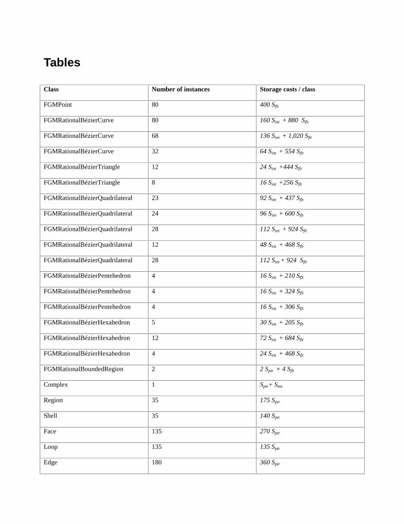
The generalized methods for representing the block with a cavity are capable of representing the desired

geometry and composition exactly. To accomplish this, the model is decomposed into FGMDomains, as

shown in Figures 9(a) and 9(b). The numbers of each FGMDomain and Radial-Edge Class and their

associated storage cost are listed in Table 1. Similarly, the data corresponding to the costs associated with

the Cell-Tuple-Graph method is listed in Table 2. By choosing to use quadratic rational pentahedral and

hexahedral FGMDomains, both the curved geometry and nonlinear composition are represented exactly. To

maintain the adjacency relationship between all of the FGMDomains, a generalized data structure is used.

The summary for storage costs for the different approaches to modeling this part are [1]:

{ }

msptrfltre

msptrfltctg

mste

mg

mmsptrfltvox

SSS S S

SSS S S

SnS

a

aaaSSSSS

+++=

+++=++=

=

+

++++=

1618789301034

958489303974

12856

32,10,min ere wh

121

lg3050100

41

63

int

int

tetrahedra

int

εε

ε

Assuming typical sizes for the primitive data types (Sint = 4 bytes, Sflt = 8 bytes, and Sptr = 4 bytes), these

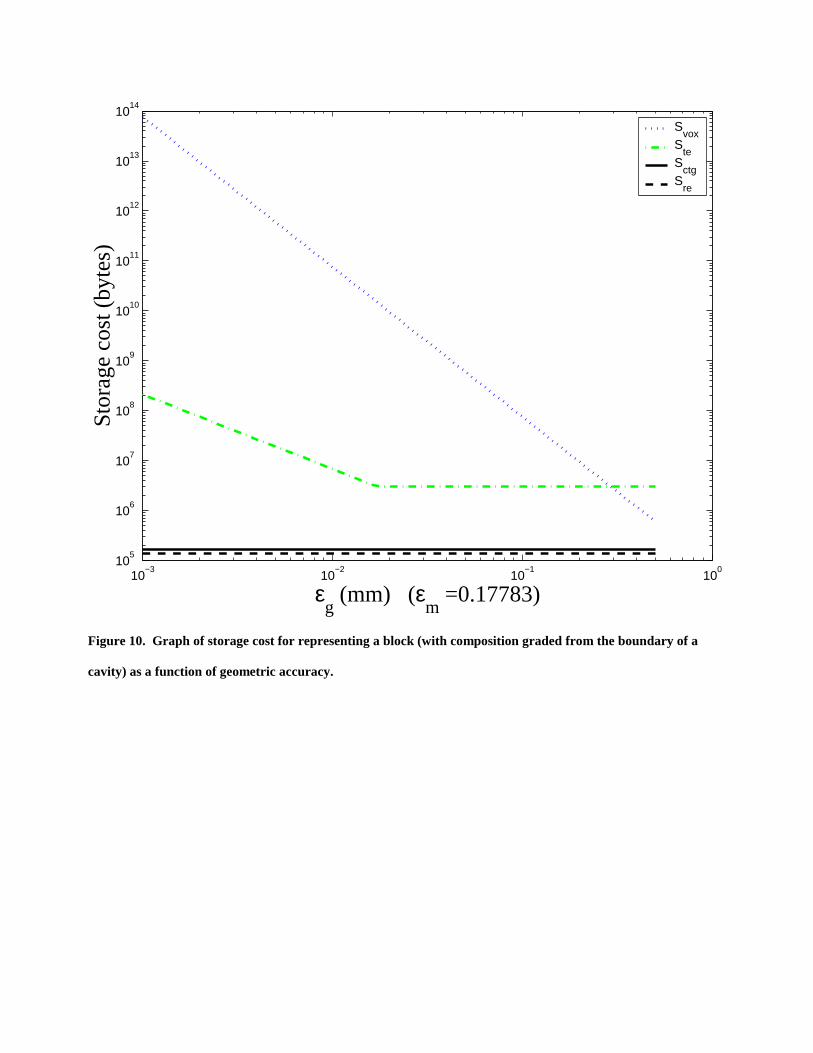
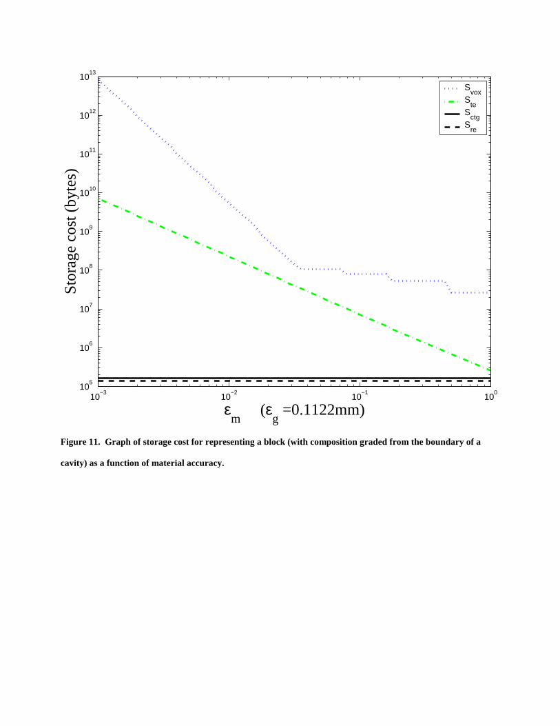
expressions are graphed in Figures 10 and 11 for a given material and geometric accuracy, respectively. In

each case, the storage costs for the Cell-Tuple-Graph and the Radial-Edge methods are constant since they

represent the intended geometry and material composition exactly. The requirements for the approximation

methods (voxel-based and tetrahedral), however, grow with increasing accuracy. In addition, each graph

may contain a break point for each approximation method at which the storage cost transitions from being a

function of the corresponding accuracy to independence of that parameter. This is due to the fact that only

one of the following four parameters are used in determining the dimensions of the voxels or the size of the

tetrahedra: geometric accuracy, material accuracy, minimum geometric feature size, or minimum material

feature size. Consider the graph in Figure 10. The geometric accuracy determines the size of the

tetrahedra for εg < 1.1x10-2 mm, while the material accuracy becomes the limiting factor for εg > 1.1x10-2 mm.

A similar explanation holds true for the graphs in Figure 11 in which the storage requirements are plotted

versus the desired material accuracy. In these cases, the breakpoints occur where the material accuracy

constraint is relaxed to the point that it no longer dominates and some other factor (usually geometric

accuracy) limits the dimensions of the voxels or tetrahedra.

In our work [1], we analyzed several other hypothetical FGM objects and quantified their storage costs in

terms of accuracy for the objects’ representation in the various data structures. Although the objects were

relatively simple in complexity, they contained features that many real objects might have, including curved

surfaces, regions of uniform and graded composition, and features such as holes or internal primitives.

They also served to illustrate how FGM models resulting from the proposed design tools might be

represented. In each case, the storage cost grew as a function of desired resolution and accuracy for

methods that require approximation (voxel-based or mesh-based), as one would expect. The generalized

approaches provided the greatest freedom in accurately representing design intent at the expense of

complexity in data structure implementation. For the generalized approach to be practical, a suitable library

of geometric and material representations (Bézier curves, surfaces, and regions, for instance) is needed

along with the necessary tools to define and interrogate the model. With such a library, the storage cost for

a generalized data structure is constant with the desired accuracy of representation and would grow only

with the number of features present in the model. With each new feature added, the complexity in

representing the topology increases, as would the amount of data needed to be stored.

Finally, it is important to note that the storage costs we determined for the voxel-based and mesh-based

methods are bounds for the memory growth as functions of geometric and material accuracy, with the

assumption of uniform meshes. Obviously, adaptive subdivision schemes should be investigated to reduce

the memory costs (as well as compression techniques such as octrees).

Conclusions and Recommendations

Data structures for representing heterogeneous, FGM objects to be fabricated with LCC were described and

analyzed in terms of their memory requirements, including a voxel-based structure, a finite-element (FE)

mesh-based approach, and generalized modeling methods such as the extension of the Radial-Edge and

Cell-Tuple-Graph data structures. All of the methods are capable of holding composition information but

each does so in a different way. Along with introducing each data structure, the storage cost for each was

derived in terms of the number of instances of each of its fundamental classes required to represent

heterogeneous objects. In order to compare data structures for modeling objects for LCC, we predicted the

storage cost for each method for several hypothetical models, one of which was presented here. Although

the models we considered were simple in nature, their curved geometries and regions of both piece-wise

constant and nonlinearly graded compositions reflect the features expected to be found in real applications.

In each case, the generalized cellular methods were found to be promising in terms of memory costs,

accurately representing the intended design. Of equal importance, although not discussed here, is the

processing efficiency of operations on these models. Based upon this work, we make the following

recommendations with regards to the limitations of existing approaches for the representation of objects with

the material information need to achieve fabrication with LCC:

• Tessellation of the volume of a model (e.g., via tetrahedral meshing) early in the design and fabrication

pathway, although expedient for testing of ideas, does not provide a long term solution for FGM

modeling for the following reasons:

1. Tessellation implies both approximation of surface geometry and material composition, which is

undesirable in general, and for realistic accuracies of approximation leads to verbose evaluated

representations, that are unattractive for general FGM modelers.

2. Although the number of elements can be reduced and approximation accuracy for surface geometry

and material composition can be improved via adaptive meshing procedures, these procedures are

difficult to implement robustly and efficiently.

3. Methods for tessellation of regions into volumetric meshes suffer from the general robustness

problem in computational geometry relating to inexact computation.

• Current approaches (based either on FE meshing or cellular decompositions) can be extended to model

FGM objects. The achievement of FGM representation, however, does not result in a general solution.

Designers still must interact with the data in a productive and efficient way. These approaches, as

defined here, permit sequential editing (first of geometry and then of composition), which is not flexible

and limits the designer’s options. FGM models are limited to low level data and operators and the

symbolic representation of the designer’s intent with respect to composition is not captured. As such,

design changes cannot be efficiently propagated.

In light of these issues, and considering their wide-spread use in existing solid modeling systems, a

generalized cellular decomposition approach to FGM modeling is a sensible starting point and is currently

being pursued by several research groups [1,10,11,32]. In addition to memory considerations, such an

approach provides the greatest opportunity for the maintenance of an unevaluated exact representation for

the geometry and composition (min(x) in Figure 5) for as long as possible along the information pathway,

providing a high level codification of the design useful in data exchange and in a general setting not

associated with a specific SFF process. Evaluation of the exact representation (to compute mout(x) in Figure

5) is performed as needed at later stages of the pathway, for visualization, design verification, or fabrication.

This can be performed at an appropriate resolution corresponding to the visualization parameters or the

limits of the specific fabrication process to be used to physically realize the model.

Furthermore, the extension of the modeling domain to represent geometric and material information with

equal importance and sophistication (Figure 2) presents additional challenges in terms of editing models. To

address these issues, further research into the simultaneous editing of geometric and material information is

needed. A promising direction for this research is the extension of feature based design (FBD) [33,34,35] to

FGM features, in which high level data of engineering significance is maintained in the model. Although the

current FBD systems carry rich information in terms of features, they only allow users to create multi-

material solids with piecewise constant composition using composite structures and assemblies. Due to the

nature of FBD, such systems usually cover a limited number of features. In order to address these

problems, the semantics of FGM features should be defined and existing FBD systems should be extended

to facilitate model creation through FGM features.

Figures

x

y

build space

model space

Bill of materials

Material m

Material m

Material m

0

1

2

z

^

^

Figure 1.

The Model Space represented by state-of-the-art solid modeling systems subdivides as Build Space into a

model’s interior and exterior with materials associated to regions.

x

y

build space

model space

mmaterial space

m

m

0

1

2z

^

^

Figure 2. The Model Space for objects consisting of graded material spans both the Build Space (X) and a

Material Space (M) in which the material variations are defined. To define an FGM object, each point in the

Build Space (x in X) must map to a composition in the Material Space (m(x) in M).

x

y

build space

model space

Intended object boundary

Modeled object boundary

εg

z

^

^

Figure 3. The maximum distance between the intended object’s boundary and the modeled boundary is the

geometric accuracy (εg) of the modeled object.

x

y

build space

model space

mmaterial space

m

m

0

1

2 εm

z

^

^

x.m(x) m(x)*

Figure 4. Visual interpretation of material accuracy, showing the difference between the desired m*(x) and the

modeled composition m(x0) at the point x0 in Build Space.

Digital model:min(x)

OrientScale

Translate

Retrospective ResampleTone Scale Adjust

Sharpen

Halftone

Physical ReconstructionFabricated part:

mout(x)

Pro

cess

Pla

nnin

gF

abri

cati

onD

esig

n

Geometric andcomposition design

Figure 5. Steps of the information flow for FGM model processing.

Figure 6. Relationships between classes for various modeling representations for FGM objects: (a) voxel, (b)

triangulated boundary representation, (c) finite-element mesh, (d) Radial-Edge, and (e) Cell-Tuple-Graph.

Figure 7. Two examples of derived FGMDomains: FGMRationalBézierCurve and

FGMRationalBézierTetrahedron.

Selected face ( )

m*=[0.5 0.5]T

m*=[1.0 0.0]T

100mm50mm

30mm

0 0.5 1 1.5 2 2.5 3 3.5 4 4.5 5

0

0.1

0.2

0.3

0.4

0.5

0.6

0.7

0.8

0.9

1

Grading of composition from cavity surface

Distance from surface (mm)

Vol

ume

frac

tion

of m

ater

ial (

mm

3 /mm

3 )

m0

m1

Figure 8. (a) Initial compositions of block and the selection of the desired faces from which the composition will

be graded. (b) Desired grading from the selected feature.

Figure 9. (a) Wireframe view of block decomposed into FGMDomains. (b) Exploded view of three

dimensional FGMDomains, colored according to their degrees of geometric and material variation.

10−3

10−2

10−1

100

105

106

107

108

109

1010

1011

1012

1013

1014

εg (mm) (ε

m =0.17783)

Stor

age

cost

(by

tes)

Svox

Ste

Sctg

Sre

Figure 10. Graph of storage cost for representing a block (with composition graded from the boundary of a

cavity) as a function of geometric accuracy.

10−3

10−2

10−1

100

105

106

107

108

109

1010

1011

1012

1013

εm

(εg =0.1122mm)

Stor

age

cost

(by

tes)

Svox

Ste

Sctg

Sre

Figure 11. Graph of storage cost for representing a block (with composition graded from the boundary of a

cavity) as a function of material accuracy.

Tables

Class Number of instances Storage costs / class

FGMPoint 80 400 Sflt

FGMRationalBézierCurve 80 160 Sint + 880 Sflt

FGMRationalBézierCurve 68 136 Sint + 1,020 Sflt


FGMRationalBézierTriangle 12 24 Sint +444 Sflt


FGMRationalBézierQuadrilateral 23 92 Sint + 437 Sflt





FGMRationalBézierPentehedron 4 16 Sint + 210 Sflt



FGMRationalBézierHexahedron 5 30 Sint + 205 Sflt



FGMRationalBoundedRegion 2 2 Sptr + 4 Sflt

Complex 1 Sptr+ Sms

Region 35 175 Sptr

Shell 35 140 Sptr

Face 135 270 Sptr

Loop 135 135 Sptr

Edge 180 360 Sptr

Vertex 80 160 Sptr

FaceUse 270 1,620 Sptr

LoopUse 270 1,620 Sptr

EdgeUse 1064 7,448 Sptr

VertexUse 1064 4,256 Sptr

Total Storage Cost 1,034Sint+8,930Sflt+16,187Sptr+Sms

Table 1. Radial-Edge and FGMDomain instances required to represent FGM block-with-cavity object exactly

and the associated storage. Multiple entries of a given class in the first column indicate the same class instanced

with different degrees of the blending functions used to define shape and/or material.

Class Number of instances Storage costs / class

FGMPoint 80 400 Sflt


FGMRationalBézierCurve 68 136 Sint + 1,020 Sflt















FGMRationalBoundedRegion 2 2 Sptr + 4 Sflt

CellTupleGraph 1 2 Sptr+ Sms

Cell 430 860 Sint+860 Sptr

Tuple 2080 2,080 Sint+18,720 Sptr

Total Storage Cost 3,974Sint+8,930Sflt+19,584Sptr+Sms

Table 2. Number of instances of each FGMDomain and Cell-Tuple-Graph class required to represent the block-with-cavity and the associated memory required. Multiple entries of a given class in the first column indicate thesame class instanced with different degrees of the blending functions used to define shape and/or material.

Acknowledgment

NSF and ONR under grants DMI-9617750, DMI-0100194 and N00014-00-1-0169. The authors thank the

referees for their comments which improved the quality of the paper.

References

1 T. R. Jackson. Analysis of Functionally Graded Material Object Representation Methods, PhD thesis, MassachusettsInstitute of Technology, January 2000. (http://czms.mit.edu/cho/3dp/publications/trj-thesis.pdf)2 H. Liu, W. Cho, T. R. Jackson, N. M. Patrikalakis, and E. M. Sachs. Algorithms for Design and Interrogation ofFunctionally Gradient Material Objects, Proceedings of 2000 ASME DETC/CIE, 26-th ASME Design AutomationConference, September, 2000, Baltimore, Maryland, USA. p.141 and CDROM, NY:ASME, 2000.3 W. Cho, E. M. Sachs, N. M. Patrikalakis, H. Liu, H. Wu, T. R. Jackson, C. C. Stratton, J. Serdy, M. J. Cima, and R.Resnick. Methods for Distributed Design and Fabrication of Parts with Local Composition Control, Proceedings of the2001 NSF Design and Manufacturing Grantees Conference, Tampa, FL, USA, January 2001.4 T. R. Jackson, N. M. Patrikalakis, E. M. Sachs, and M. J. Cima. Modeling and Designing Components with LocallyControlled Composition. In D. L. Bourell et al, editor, Solid Freeform Fabrication Symposium, pages 259-266, Austin,Texas. The University of Texas, August 10-12 1998.5 T. R. Jackson, H. Liu, N. M. Patrikalakis, E. M. Sachs, and M. J. Cima. Modeling and Designing FunctionallyGraded Material Components for Fabrication with Local Composition Control. Materials and Design, 20(2/3):63-75,June 1999.6 A. Kaufman, D. Cohen, and R. Yagel. Volume Graphics. Computer, 26(7):51-64, July 1998.7 S. Manohar. Advances in volume graphics, Computers and Graphics, 23(9):73-84, August 1999.8 V. Chandru, S. Manohar, and C. E. Prakash. Voxel-based modeling for layered manufacturing. IEEE ComputerGraphics and Applications, 15(6):42-47, 1995.9 J. Pegna and A. Safi. CAD Modeling of Multi-Modal Structures for Freeform Fabrication, 1998. Presentation atSolid Freeform Fabrication Symposium, Austin, Texas. The University of Texas, August 12-14, 1998.10 S.-M. Park, R. H. Crawford, and J. J. Beaman. Volumetric Multi-Texturing for Functionally Gradient MaterialRepresentation. In D. C. Anderson and K. Lee, editors, Sixth ACM Symposium on Solid Modeling and Applications,June 6-8, 2001, pages 216-224. New York, 2001. ACM SIGGRAPH.11 V. Kumar and D. Dutta. An Approach to Modeling Multi-Material Objects. In C. Hoffmann and W. Bronsvort,editors, Fourth Symposium on Solid Modeling and Applications, Atlanta, Georgia, May 14-16, 1997, pages 336-353,New York, 1997. ACM SIGGRAPH.12 V. Kumar and D. Dutta. An Approach to Modeling and Representation of Heterogeneous Objects. Journal ofMechanical Design, 120:659-667, December 1998.13 V. Kumar, D. Burns, D. Dutta, and C. Hoffmann. A Framework for Object Modeling. Computer-Aided Design,31(9):541-556., August, 1999.14 L. Bardis and N. M. Patrikalakis. Topological Structures for Generalized Boundary Representations, MIT SeaGrant Report 94-22, Cambridge, MA, 1994.15 E. Brisson, Representing Geometric Structures in d Dimensions: Topology and Order. Discrete andComputational Geometry. 9: 387-426. 199316 C.-Y. Hu, N. M. Patrikalakis, and X. Ye. Robust Interval Solid Modeling: Part I, Representations. Computer AidedDesign. 28(10):807—817. October 199617 R. Ulichney. Digital Halftoning. Cambridge. MIT Press. 1987.18 D. L. Bourell, R. H. Crawford, H. L Marcus, J. J. Beaman and J. W. Barlow, Selective Laser Sintering of Metals.In Proceedings of the 1994 ASME Winter Annual Meeting. Chicago, IL. Pages 519-528. November 6-11 1994.

19 E. Sachs, E. J. Haggerty, M. Cima, and P. Williams. Three-Dimensional Printing U.S. Patent No. 5,204,055.April 20 1993.20 L. E. Weiss, R. Merz, F. B. Prinz, G. Neplotnik, and P. Padmanabhan, L. Schultz, and K. Ramaswami. ShapeDeposition Manufacturing of Heterogeneous Structures. SME Journal of Manufacturing Systems. 16(4):239-248.1997.21 K. J. Jakubenas, J. M. Sanchez, and H. L. Marcus. Multiple Material Solid Free-form Fabrication by Selective AreaLaser Deposition. Materials and Design. 19(1/2):11-18. Elsevier Science. 1998.22 I. Jackson, H. Xiao, M. Ashtiani, and L. Berben. Stereolithography Model in Presurgical Planning of CraniofacialSurgery. In D. L. Bourell et al, editor, Solid Freeform Fabrication Symposium. Pages 9-14. Austin, Texas. August12-14 1996. The University of Texas23 J. Mazumder, J. Choi, K. Nagarathnam, J. Koch and D. Hetzner, "Direct Metal Deposition of H13 Tool Steel for 3-D Components: Microstructure and Mechanical Properties," Journal of Metals, 49(5):55-60. 1997.24 A. Marsan, V. Kumar, and D. Dutta,. and M. Pratt. An Assessment of Data Requirements and Data TransferFormats for Layered Manufacturing. 1999. NISTIR 6216. Gaithersburg, Maryland. U.S. Department of Commerce.25 K. J. Weiler. The Radial Edge Structure: A Topological Representation for Non-Manifold Geometric Modeling. InM. J. Wozny, H. McLaughlin, and J. Encarnacao, editors, Geometric Modeling for CAD Applications. Pages 3-36.Elsevier Science Publishers, Holland, 1986.26 E. L. Gürsöz, Y. Choi, and F. B. Prinz. Vertex-Based Representation of Non-Manifold Boundaries. In M. J.Wozny, J. U. Turner and K. Preiss, editors, Geometric Modeling for Product Engineering. Pages 107-130. ElsevierScience Publishers, Holland, 1990.27 J. R. Rossignac and M. A. O'Connor. SGC: A Dimension-Independent Model for Point Sets with Internal Structuresand Incomplete Boundaries. In M. J. Wozny, J. U. Turner and K. Preiss, editors, Geometric Modeling for ProductEngineering. Geometric Modeling for Product Engineering. Pages 145-180. 1990. Holland, Elsevier SciencePublishers.28 G. Farin. Curves and Surfaces for Computer Aided Geometric Design - A Practical Guide, 3rd Edition, AcademicPress, Inc., San Diego, CA.29 S. T. Tuohy, J. W. Yoon, and N. M. Patrikalakis. Trivariate Parametric B-Splines for Visualization of Ocean Data.In Proceedings of Oceans ’95: Challenges of Our Changing Global Environment. Volume 3. Pages 1601-1608. SanDiego, CA. October 3, 1995. 1601-1608. MTS/IEEE Oceanic Oceanic Engineering Society.30 L. Fang and D. C. Gossard. Multidimensional Curve Fitting to Unorganized Data Points by NonlinearMinimization. Computer Aided Design. 27(1):46-58. 1995.31 H.-P. Seidel Symmetric Triangular Algorithms for Curves. Computer Aided Geometric Design. 7:57-67. 1990.32 K. H. Shin, and D. Dutta. Constructive Representation of Heterogeneous Objects. Journal of Computing andInformation Science in Engineering. 1(3):205-217. 2001. ASME33 J. Shah and M. Mäntylä. Parametric and Feature-Based CAD/CAM, John Wiley, Inc., 1995.34 X. Qian. Feature Methodologies for Heterogeneous Object Realization, PhD thesis, The University of Michigan,April 2000.35 X. Qian and D. Dutta. Feature Based Fabrication in Layered Manufacturing. Journal of Mechanical Design.123(3):337-345. 2001. ASME.

Memory Analysis of Solid Model Representations for ...

Documents

Transcript of Memory Analysis of Solid Model Representations for ...