
MemoriaTesis Ricardo Granizo V1 20180416 AC y DC · 2020. 6. 1. · *uhhwlqjv , zrxog olnh wr...
264
UNIVERSIDAD POLITÉCNICA DE MADRID ESCUELA TÉCNICA SUPERIOR DE INGENIEROS INDUSTRIALES New methods and protection systems for AC and DC power networks Doctoral Thesis To obtain the Title of Doctor in Industrial Engineering Ricardo Granizo Arrabé Master in Electrical Engineering by Universidad Politécnica de Madrid 2018
Transcript of MemoriaTesis Ricardo Granizo V1 20180416 AC y DC · 2020. 6. 1. · *uhhwlqjv , zrxog olnh wr...

UNIVERSIDAD POLITÉCNICA DE MADRID
ESCUELA TÉCNICA SUPERIOR DE INGENIEROS
INDUSTRIALES
New methods and protection systems
for AC and DC power networks
Doctoral Thesis
To obtain the Title of Doctor in Industrial Engineering
Ricardo Granizo Arrabé
Master in Electrical Engineering by Universidad Politécnica de Madrid
2018


Department of de Electronics, Electrical Engineering and Industrial Computing
ESCUELA TÉCNICA SUPERIOR DE INGENIEROS
INDUSTRIALES
New methods and protection systems
for AC and DC power networks
Doctoral Thesis
To obtain the Title of Doctor in Industrial Engineering
Author: Ricardo Granizo Arrabé Master in Electrical Engineering by Universidad Politécnica de Madrid
Director: Carlos Antonio Platero Gaona Doctor Industrial Engineer by Universidad Politécnica de Madrid

Tribunal
Named by the Magnificent and Excellent Rector of the Universidad
Politécnica de Madrid on XX de February 2018.
President: Dr. Carlos Veganzones Nicolás
Secretary: Dr. Francisco Blazquez García
Vocals: Dr. Konstantinos Gyftakis
Dr. Óscar Duque Pérez
Dr. José Alfonso Antonino Daviu
Suplentes: Dr. Santiago Arnaltes Gómez
Dr. José Luís Rodríguez Amenedo

Greetings
I would like to mention relevant persons that have contributed to make this work
come true from the very beginning to the end.
To Carlos Platero Gaona, Director of this Doctoral Thesis. Without his continuous
support and expert criteria together with his accurate definition of the most important
aspects to be taken into account in the development of new ideas, redaction of new
patents, evaluation of simulation results and laboratory tests, these studies would have
never ended with so many positive aspects. I also to highlight his priceless human support
when my contractual situation inside the Universidad Politécnica de Madrid was changed
to an insignificant role at the Electrical Department of the ETSIDI where I was full time
professor. Many thanks for ever.
To all the professors at the ETSII and ETSIDI that did encourage me
continuously to finish the doctorate studies and to all the doctorate colleagues at ETSII
and the laboratory staff whose excellent attitude towards me made me feel very happy
sharing laboratory tests, ideas, problems, very active and hectic lunches, etc. Thanks so
much. To Fernando Álvarez Gómez who helped me with at any time with his great
attitude towards me, many thanks. To Alejandro Viñuelas Fernández and David
Talavera Miguel who gave me light many and crucial times fixing all problems I had
with my pc. To Santiago Bernal Parrondo who helped me with the last DC laboratory
tests.
To an endless number of friends that gave to me their support and care. I don´t
include your names because I am sure that I will forget some of you and that will make
me uncomfortable.
To my family, my parents Mary Cruz and Juan Manuel, my aunt Mercedes, my
cousins Susana and Filippo, my wife Chang-Yuan and my little daughter Celia, and
grandparents Patrocinio and Alfonso. I can´t express or describe accurately my thanks
to you for letting me have the most important things I have got in live: your education and
endless care.
Madrid, March 2018.

Universidad Politécnica de Madrid ETSI Industriales Ricardo Granizo Arrabé Doctoral Thesis
I
Abstract
This thesis focuses on the study and development of new protection methods and systems for power cables used in both AC and DC grids, from generation to distribution or transmission power networks.
In AC networks there are many protection functions that allow clearing ground faults from the measurements of currents and voltages obtained from the measurement devices as current transformers, voltage transformers or both. In some applications at transition stations from overhead lines to underground lines, the up and running protection relays can detect the ground fault and develop a correct tripping of the circuit breakers associated to such overhead or underground line. Those protection relays don´t know actually if the ground fault has happened at the overhead side or at the underground side. This circumstance is extremely important in order to allow having auto-reclosing attempts or not. If the order to switch on again the circuit breakers and restore power supply is developed under active ground fault conditions, the consequences can be dramatic if the permanent ground fault is at the underground line side. If the isolation and dielectric characteristics of the underground cables were already relatively damaged, a direct attempt to switch on the circuit breakers will cause a permanent damage in such cables forever and they will have to be replaced by new ones with the consequent lose of power supply for long time.
This work proposes new protection methods that identifies if the ground fault has happened at the overhead line side or at the underground cable side. It can release the autoreclosing attempts to minimize the power oscillations of the grid as much as possible when the ground fault has happened at the overhead line side, or block them when the ground fault happened at the underground cable side. So far, no protection relays manufacturers have developed any relay with these characteristics, just the commonly named as SOTF (Switch On To Fault) which is described in the state of the art.
During the development of this thesis, some patents which are property of the Universidad Politécnica de Madrid have been obtained for both AC applications. One of them (P201431962: Method to Determine a Ground Fault Emplacement in Circuits with Transitions Overhead Line to Underground Cable Line) has been recently licensed (dated on 23-January-2017) to DSF Tecnologías para Motores y sus Aplicaciones, S.L.with contract nº NL170020064, as they are the Spanish Distributor of the German company Woodward-Seg which designs, develops and manufactures protection relays for low, medium and high AC voltage networks for the last forty years, and showed high interest in including the concepts of this patent in a new protection relay.
One of the challenges of this work was to develop new cable protection methods that could be implemented in protection relays in the easiest possible way and, at the same time, with the lowest possible investments. All new methods request the application of current and voltage transformers or sensors actually in use worldwide.
In DC grids there are not so many protection functions in operation because high voltage DC networks are not used widely. Nevertheless, power transmission lines also have protection systems to clear ground faults. Normally, DC power links are one-to-one and the main

Universidad Politécnica de Madrid ETSI Industriales Ricardo Granizo Arrabé Doctoral Thesis
XIII
protections are included in the AC/DC converter at the DC side. Multiterminal grids are not installed in a great deal so no big experience is known when facing up the challenge of erecting these kinds of new DC grids.
Thinking in new multiterminal grids in DC, more protections functions must be developed in order to grant full selectivity in such grids.
New protection concepts for DC cable power networks have been evaluated, simulated and tested with good results for ground faults at the positive or negative cables.
In the same way that happened with the research for AC networks, during the development of this thesis, other patents which are property of the Universidad Politécnica de Madrid were obtained for DC power cable protection.
The most important task of this work was to develop new protection methods that could be implemented in protection relays in the easiest possible way and, at the same time, with the lowest possible investments. All new methods request the application of standard current sensors actually in use worldwide.
This document starts with the description of the actual protection functions used for detecting and clearing ground faults at AC and DC power networks. It follows a complete description of the new detecting methods that includes their operating principles.
The simulation tool used for signal analysis of currents and voltages is also described including simulation and laboratory test results.
At the end of this document, the main conclusions and improvements in cable ground fault detection for AC and DC networks developed in this work are written. Future research lines are also described and included.

Universidad Politécnica de Madrid ETSI Industriales Ricardo Granizo Arrabé Doctoral Thesis
III
Index
1. INTRODUCTION. .................................................................................................................... 1
1.1. Motivation of the thesis. .............................................................................................. 2
1.2. Main objectives of the thesis. ...................................................................................... 3
1.3. Development of the thesis. ........................................................................................... 4
2. STATE OF THE ART IN GROUND FAULTS LOCATION IN AC POWER SYSTEMS.. .. 6
2.1. Types of faults and basics of protection philosophy.. .................................................. 8
2.1.1. Methods for ground faults location. ........................................................................... 14
2.1.2. Methods that use the phase information of zero sequence currents and voltages…. . 15
2.1.3. Methods that use the Wavelet Transformation and Travelling Wave Theory…….. . 16
2.1.4. Methods that use algorithms based on two end terminal measurements ................... 18
2.2. Current transformers used in protection systems.. ..................................................... 18
2.2.1. Performance of a current transformers atn steady state when there is no fault condition… .............................................................................................................................. 19
2.2.2. Example of calculation of factor R.… ....................................................................... 21
2.2.3. Performance of a current transformer in transients .................................................... 23
2.2.4. Examples of calculation of I2.and λ ........................................................................... 25
2.2.5. Connections of current transformers for detecting ground fault currents .................. 27
2.3. Grounding systems of power cable shields.. .............................................................. 31
2.3.1. Introduction. ............................................................................................................... 31
2.3.2. Grounding of both ends of the shields. Solid-Bonding (SB).. ................................... 35
2.3.3. Grounding at only one end of the shields. Single-Point (SP) or Mid-Point (MP). .... 38
2.3.4. Cross-Bonding connection (CB). ............................................................................... 44
2.3.5. Transposition of conductors and shields. ................................................................... 48
2.3.6. Selection of voltage limiters on shields. .................................................................... 49
2.4. The Wavelet Transformation.. ................................................................................... 54
2.4.1. Introduction. ............................................................................................................... 54
2.4.2. Representation of signals in the time domain. ........................................................... 55
2.4.3. Fourier and his transformation. .................................................................................. 56
2.4.4. The Wavelet Transform. ............................................................................................ 57
2.4.5. Fundamentals of the Wavelet Transform. .................................................................. 58
2.4.6. Main application of the Wavelet Transform. ............................................................. 60
2.4.7. Example of analysis using the Wavelet Transform ................................................... 61
2.4.8. Main Wavelet families. .............................................................................................. 64
Universidad Politécnica de Madrid ETSI Industriales Ricardo Granizo Arrabé Doctoral Thesis
XIII
2.4.9. Detection of disturbances. .......................................................................................... 66
2.4.10. Signal detection of events and changes. .................................................................... 67
2.4.11. Selection of wavelet function. ................................................................................... 67
2.4.12. Example of mother wavelet selection. ....................................................................... 69
2.5. Failure ground fault location at combined overhead-cable lines in ANSI 21 and ANSI 67N protection relays.. ............................................................................................................ 71
2.5.1. Theoretical study........................................................................................................ 72
2.5.2. Conclusion. ................................................................................................................ 79
2.6. Switch-on to fault schemes in protection functions.. ................................................. 80
2.6.1. Application of SOFT protection schemes. ................................................................. 80
2.6.2. Common SOFT protection schemes. ......................................................................... 81
2.6.3. Auto-reclosing SOFT protection schemes. ................................................................ 82
2.6.4. Example of SOFT protection scheme. ....................................................................... 83
2.7. Glossary second chapter.. .......................................................................................... 84
3. STATE OF THE ART IN GROUND FAULTS LOCATION IN DC PROTECTION SYSTEMS.. ................................................................................................................................. 88
3.1. Introduction to HVDC transmission systems. ........................................................... 90
3.1.1. Characteristics of HVDC transmission systems. ....................................................... 91
3.1.2. HVDC transmission systems. principal network configurations. ............................. 98
3.1.2.1.HVDC with single-pole configuration ...................................................................... 98
3.1.2.1.1.Single-pole HVDC with ground or sea return path ................................................ 98
3.1.2.1.2.Single-pole HVDC with ground or sea return path ................................................ 99
3.1.2.2. HVDC with double-pole configuration ................................................................... 99
3.1.2.2.1. Double-pole HVDC with ground return path ..................................................... 100
3.1.2.2.2. Double-pole HVDC with metallic ground return path ....................................... 100
3.1.2.2.3. Double-pole HVDC without ground return path ................................................ 101
3.1.2.3. HVDC with homopolar configuration ................................................................... 102
3.1.3. Protections in HVDC transmission power systems. ............................................... 102
3.1.3.1.Restrictions in protection systems used in transmission HVDC ............................. 103
3.1.3.2.Clearing times for fault currents in transmission HVDC ........................................ 103
3.1.3.3.Options for clearing fault currents in transmission HVDC ..................................... 104
3.1.4. Voltage measurement in HVDC systems. .............................................................. 108
3.1.5. Methods for ground fault detection in HVDC networks. ........................................ 112
3.1.5.1. Analysis of the initial variation of current di/dt .................................................... 112
3.1.5.1.1. Fault detection using the rate of current rise ...................................................... 114
3.1.5.2. Analysis of the rate of change of voltage (ROCOV) ............................................ 114

Universidad Politécnica de Madrid ETSI Industriales Ricardo Granizo Arrabé Doctoral Thesis
XIII
3.1.5.3. Handshaking method ............................................................................................. 115
3.1.6. Mechanical DC circuitbreakers. ............................................................................. 117
3.2. Glossary third chapter. ............................................................................................. 119
4. NEW PROTECTION METHODS FOR AC POWER SYSTEMS. ................................... 121
4.1. Novel method for blocking the auto-reclosing maneouvres in combined overhead-cable lines. ............................................................................................................................. 123
4.1.1. Combined overhead-cable line with YN and D transformer connections. .............. 123
4.1.2. Impedances of cables and shields. ........................................................................... 124
4.1.3. Balanced system: General equations for SB shield connections. ............................ 124
4.1.4. Principles of the novel auto-reclosing blocking method for distribution networks. 126
4.1.4.1. Analysis of the angle differences between currents in conductors and currents in shields. ................................................................................................................................. 127
4.1.4.2. Algorithm of the new auto-reclosing blocking method. .......................................... 128
4.1.4.3. Simulation results: analysis.. ................................................................................... 129
4.1.4.4. Angle difference analysis in distribution networks solidly grounded at the overhead side and isolated at the cable end side.. ................................................................................. 131
4.1.4.5. Wavelet analysis in a distribution system solidly grounded at the overhead side and isolated at the cable end side.. ............................................................................................... 134
4.1.4.6. Test results.. ............................................................................................................. 136
4.1.4.7. Angle analysis of the experimental distribution system solidly grounded at the overhead side and isolated at the cable end side.. ................................................................. 139
4.1.4.8. Wavelet analysis of the experimental distribution system solidly grounded at the overhead side and isolated at the cable end side.. ................................................................. 142
4.1.4.9. Conclusions.. ............................................................................................................ 145
4.2. Novel protection method for detection of ground faults in cables used is combined overhead-cable lines in power systems. ................................................................................ 146
4.2.1. Principles of operation. ............................................................................................ 147
4.2.2. Simulation results. .................................................................................................. 149
4.2.2.1. Ground fault at the cable line side.. ......................................................................... 151
4.2.2.2. Ground fault at the overhead line side.. ................................................................... 155
4.2.3. Experimental results. ............................................................................................... 159
4.2.3.1. Experimental set-up.. ............................................................................................... 159
4.2.3.2. Ground fault at the cable line side.. ......................................................................... 161
4.2.3.3. Ground fault at the overhead line side.. ................................................................... 162
4.2.3.4. Conclusions.. ............................................................................................................ 164
4.3. Novel ground fault non directional selective protection method for isolated distribution networks. ............................................................................................................ 165
4.3.1. Actual protection systems used in ungrounded distribution networks. ................... 166

Universidad Politécnica de Madrid ETSI Industriales Ricardo Granizo Arrabé Doctoral Thesis
XIII
4.3.1.1.Residual overvoltage protection (ANSI 59N).. ......................................................... 166
4.3.1.2. Non-directional ground faut current protection (ANSI 51).. ................................... 166
4.3.1.3. Directional ground fault currentprotection (ANSI 67N).. ........................................ 167
4.3.1.4. Measuring the isolation resistance.. ......................................................................... 168
4.3.2. Principle of operation of the new selective ground fault detection technique. ........ 168
4.3.2.1.Ground fault detection method formain substations.. ............................................... 169
4.3.2.2.Ground fault detection algorithm for secondary substations.. ................................... 169
4.3.2.3. Examples of application of the new method. ........................................................... 171
4.3.2.3.1.Ground fault in an outgoing line of any secondary substation.. ............................. 171
4.3.2.3.2. Ground fault in a kine that connects a main substation with a secondary substation.. 173
4.3.3. Analysis of simulation results. ................................................................................. 175
4.3.3.1.Main substations.. ...................................................................................................... 175
4.3.3.2.Secondary substations.. ............................................................................................. 177
4.3.4. Experimental results. ............................................................................................... 179
4.3.4.1.Experimental setup.. .................................................................................................. 179
4.3.4.2.Three lines with identical lenghts.. ............................................................................ 181
4.3.4.3.Three lines with different lenghts.. ............................................................................ 182
4.3.4.4.Conclusions.. ............................................................................................................. 185
4.4. Glossary fourth chapter. ........................................................................................... 186
5. NEW PROTECTION METHODS FOR DC POWER SYSTEMS. ............................. 189
5.1. Introduction. ............................................................................................................. 191
5.2. Matlab-Simulink model implemented for new protection methods for HVDC power cable systems. ........................................................................................................................ 191
5.3. Differential ground fault detection method for DC insulated cables. ...................... 196
5.3.1. Background of the method. ...................................................................................... 196
5.3.2. Description of the method. ....................................................................................... 197
5.3.3. Simulatin results: differential ground fault detection method. ................................ 198
5.3.4. Experimental model implemented in laboratory. ..................................................... 202
5.3.5. Experimental results: Ground fault. ......................................................................... 204
5.4. Directional ground fault detection method for DC insulated cables. ....................... 206
5.4.1. Background of the method. ...................................................................................... 206
5.4.2. Description of the method. ....................................................................................... 207
5.4.3. Simulatin results: directional ground fault detection method. ................................. 209
5.4.4. Experimental results: Ground fault. ......................................................................... 211
5.5. Identification of swithcing-on currents in DC insulated cables. .............................. 212

Universidad Politécnica de Madrid ETSI Industriales Ricardo Granizo Arrabé Doctoral Thesis
XIII
5.5.1. Description of the method. ....................................................................................... 213
5.5.2. Simulation results: switching-on currents in DC insulated cables. .......................... 214
5.5.3. Experimental results: switching-on commands. ...................................................... 216
5.6. Glossary fifth chapter. .............................................................................................. 219
6. CONCLUSIONS AND FUTURE LINES OF RESEARCH. ......................................... 221
6.1. Conclusions. ............................................................................................................. 223
6.2. Future lines of research. ........................................................................................... 225
6.3. Publications. ............................................................................................................. 225
References. ............................................................................................................................... 230
Figures:
Fig. 1: Basic SEF network with overcurrent protection relay.. ..................................................... 9 Fig. 2: Basic DEF network with overcurrent protection relays ................................................... 10 Fig. 3: Basic back-up protection system definition. .................................................................. 210 Fig. 4: Basic tripping times of back-up protections in DEF networks. ....................................... 12 Fig. 5: Basic tripping times of back-up protections in mesh SEF networks. .............................. 12 Fig. 6: Protected zones not overlapped. ...................................................................................... 13 Fig. 7: Protected zones overlapped. ............................................................................................ 14 Fig. 8: Overlapping around protection relay R1.......................................................................... 14 Fig. 9: Wavelet transformation. Frequency bands related to decomposition steps.. ................... 17 Fig. 10: Equivalent circuit for a real current transformer. ........................................................... 19 Fig. 11: Excitation current for 500/1 A current transformer. ...................................................... 21 Fig. 12: Current transformer equivalent circuit. .......................................................................... 22 Fig. 13: Equivalent circuit for transient analysis of current transformers. .................................. 24 Fig. 14: Currents I1, I2, 𝜆 and saturation level.. ........................................................................... 27 Fig. 15: Holmgreen Circuit.. ....................................................................................................... 28 Fig. 16: Correct grounding connection of shields.. ..................................................................... 29 Fig. 17: Incorrect grounding connection of shields.. ................................................................... 30 Fig. 18: Magnetic field created by an electrical current. ............................................................. 32 Fig. 19: Circulating currents induced in shields .......................................................................... 33 Fig. 20: Induced Foucoult currents in shields. ............................................................................ 33 Fig. 21: Induced currents in shields. ........................................................................................... 34 Fig. 22: Solid-bonding arrangement (SB).. ................................................................................. 37 Fig. 23: Solid-bonding arrangement (SB) with intermediate joint.. ............................................ 37 Fig. 24: Solid-bonding arrangement (SB) with transposition of conductors.. ............................. 37 Fig. 25: Induced voltage in solid-bonding arrangement (SB).. ................................................... 38 Fig. 26: Single-point (SP) connection.. ....................................................................................... 40 Fig. 27: Mid-point (MP) connection.. ......................................................................................... 41 Fig. 28: Shields with n-strechts in SP connection concatenated.. ............................................... 41
Fig. 29: Induced voltage in single-point (SP) connection.. ......................................................... 42 Fig. 30: Local and absolute voltages in a SP system.. ................................................................. 42 Fig. 31: Surge-arrester and LTP emplacements in cable with SP connection. ............................ 44 Fig. 32: Cross-bonding (CB) connection.. .................................................................................. 46

Universidad Politécnica de Madrid ETSI Industriales Ricardo Granizo Arrabé Doctoral Thesis
XIII
Fig. 33: Induced voltage in a cross-bonding (CB) connection.. .................................................. 46 Fig. 34: Induced voltage in a shields circuit with CB connection.. ............................................. 47 Fig. 35: Sectioned cross-bonding arrangement (CBS).. .............................................................. 47 Fig. 36: Continuous cross-bonding (CCB) connection.. ............................................................. 48 Fig. 37: Transposition of conductors and shields.. ...................................................................... 49 Fig. 38: Single pole grounding box.. ........................................................................................... 52 Fig. 39: Three pole grounding box.. ............................................................................................ 53 Fig. 40: Single pole grounding box with LPT. ............................................................................ 53 Fig. 41: Three pole shields transposition box (CB).. ................................................................... 54 Fig. 42: Temporal representation. Time domain. ........................................................................ 55 Fig. 43: Signal analyzed: 𝑦(𝑡) = 0.7 · 𝑠𝑖𝑛(100 · 𝜋 · 𝑡) + 𝑠𝑖𝑛(240 · 𝜋 · 𝑡).. .............................. 56 Fig. 44: Fourier transform of the signal: 𝑦(𝑡) = 0.7 · 𝑠𝑖𝑛(100 · 𝜋 · 𝑡) + 𝑠𝑖𝑛(240 · 𝜋 · 𝑡).... ..... 57 Fig. 45: Signal analysis using Wavelet Daubechies dB4.. .......................................................... 58 Fig. 46: Signal analysis using Wavelet Coiflet1. ........................................................................ 59 Fig. 47: Signal analysis using Wavelet Coiflet5.. ....................................................................... 59 Fig. 48: Sample electrical circuit for analysis of swicthing-on a capacitor.. ............................... 61 Fig. 49: Sample electrical circuit for analysis: Voltage at node A. Connection of capacity.. ..... 62 Fig. 50: Wavelet transform of the voltage at node A when using a "Daubechies 4" transformation; First level of detail D1; Connection of capacity.. ............................................. 62 Fig. 51: Sample electrical circuit for analysis: Connection of inductance.. ................................ 63 Fig. 52: Sample electrical circuit for analysis; Voltage at node A; Connection inductance.. ..... 63 Fig. 53: Wavelet transform of the voltage at node A when using a "Daubechies 4" transformation; First level of detail D1; Connecting inductance.. .............................................. 64 Fig. 54: Wavelet Haar.. ............................................................................................................... 65 Fig. 55: Wavelet Daubechies. ..................................................................................................... 65 Fig. 56: Wavelet Coiflet. ............................................................................................................. 66 Fig. 57: Single-phase ground fault detection in a 220 kV grid using a Daubechies db6 wavelet.. ..................................................................................................................................................... 66 Fig. 58: Signal with perturbation analyzed.. ............................................................................... 69 Fig. 59: Defect current and selection of mother wavelet.. .......................................................... 71 Fig. 60: Defect current and selection of mother wavelet. Zoom of the coefficients db3 - cD1 obtained.. ..................................................................................................................................... 71 Fig. 61: Power distribution network rated 20 kV: dimensions of tower used.. .......................... 73 Fig. 62: Ground fault at the end of the overhead line side.. ........................................................ 74 Fig. 63: Relay Characteristic Angle (RCA) in solidly grounded power distribution networks.. 78 Fig. 64: Example of SOFT protection scheme.. .......................................................................... 83 Fig. 65: Basic HVDC system. ..................................................................................................... 91 Fig. 66: Current distribution in underground cable. .................................................................... 91 Fig. 67: Voltage distribution in overhead conductor. .................................................................. 92 Fig. 68: Transmission capacity in HVDC´s and HVAC´s. Courtesy by Universidad de Valladolid. ................................................................................................................................... 93 Fig. 69: Power flow in AC systems. ............................................................................................ 94 Fig. 70: Power Transmission in DC systems. ............................................................................. 95 Fig. 71: Estimation costs: comparison between HVAC and HVDC power transmission systems. Courtesy by Universidad de Valladolid. ..................................................................................... 96 Fig. 72: HVDC transmission line versus HVAC transmission line. Courtesy by Power Engineers 2009.. ........................................................................................................................................... 97 Fig. 73: HVDC: single-Pole connection with ground/sea return path.. ....................................... 95

Universidad Politécnica de Madrid ETSI Industriales Ricardo Granizo Arrabé Doctoral Thesis
XIII
Fig. 74: HVDC: single-Pole connection with metal return path. ................................................ 99 Fig. 75: HVDC: double-Pole connection with ground return path. .......................................... 100 Fig. 76: HVDC: double-Pole connection with metallic return path. ......................................... 101 Fig. 77: HVDC: double-Pole connection without return path. .................................................. 101 Fig. 78: HVDC: homopolar connection. ................................................................................... 102 Fig. 79: HVDC: Local position fault currents switching-off. ................................................... 105 Fig. 80: HVDC: IGBTs blocking. ............................................................................................. 105 Fig. 81: HVDC: Busbar disconection. ...................................................................................... 106 Fig. 82: HVDC: Partial grid disconenction. .............................................................................. 106 Fig. 83: HVDC: Complete grid disconnection. ......................................................................... 107 Fig. 84: Protection zones for an HVDC used in long distance power transmission. Courtesy by SIEMENS AG, 2011. ................................................................................................................ 108 Fig. 85: Voltage divider RC used in HVDC: frequency response versus ratio error (%). ........ 109 Fig. 86: HVDC: Typical connections for a voltage divider RC.. .............................................. 109 Fig. 87: Hibrid-Optical DC current measurement. Courtesy by SIEMENS AG, 2011. ............ 112 Fig. 88: HVDC network considered for di/dt analysis. ............................................................. 113 Fig. 89: HVDC: areas of di/dt for different transients. ............................................................. 114 Fig. 90: Typical mechanical DC circuit breaker structure. ....................................................... 117 Fig. 91: Cable composition (a) and flat disposal (b). (ric) internal conductor radius, (roc) external conductor radius, (ris) internal conductor screen, (ros) external screen radius,(rS) average screen radius, (SCS) distance between axes of conductor and screen, (tps) external cover thickness.. .. 123 Fig. 92: Standard shields connection for SB applications. (Ia, Ib, Ic) Currents in Conductors,( Isa, Isb, Isc) Currents in Shields, (R1, R2) Ground Resistances at both ends of shields, (U) Voltage Difference between shield terminals.. ....................................................................................... 125 Fig. 93: Currents measured of the cables in the active conductors and in their shields.. .......... 127 Fig. 94: Algorithm of the new auto-reclosing method.. ............................................................ 129 Fig. 95: New auto-reclosing blocking method: Model implemented.. ..................................... 130 Fig. 96: Angle differences with ground fault at the overhead side in phase L1.. ...................... 131 Fig. 97: Angle differences with ground fault at the cable side in phase L1.. ............................ 132 Fig. 98: Wavelet dB2-1 - cD1 coefficients of the angle differences signals with ground fault in phase L1 at the overhead side 12 km from the transition.. ........................................................ 134 Fig. 99: Wavelet db2-1 - cD1 coefficients of the angle differences signals with ground fault in phase L1 at the cable side 300 m from the transition.. .............................................................. 135 Fig. 100: Experimental set-up. (1: Protection relays; 2: Auxiliary power supply; 3: Power supply; 4: Loads; 5: Ground defect switch; 6: Transformer; 7: PC; 8: Cables; 9: Line modules; 10: Line module box; 11: RLC parameters of the line modules used).. .................................... 137 Fig. 101: Ground defect positions: (A: at the end of the cable, B: between first and second section of the cables; C: between the second and third section of the cables; D: in the transition at the end of the cables; E: between the first and second tram of the line modules; F: behind the two line modules).. .................................................................................................................... 138 Fig. 102: Ground defect positions: schematic representation.. ................................................. 138 Fig. 103: Angle differences with ground fault at the overhead side in phase L1. Fault point E.. ................................................................................................................................................... 139 Fig. 104: Angle differences with ground fault at the cable side in phase L1. Fault point C.. ... 140 Fig. 105: Wavelet analysis of the angle differences with ground fault at the overhead side in phase L1. Fault point E.. ........................................................................................................... 143 Fig. 106: Wavelet analysis of the angle differences with ground fault at the overhead side in phase L1. Fault point C.. ........................................................................................................... 143

Universidad Politécnica de Madrid ETSI Industriales Ricardo Granizo Arrabé Doctoral Thesis
XIII
Fig. 107: Transmission system with overhead-cable transition station. (1) Active conductor of Power Cables, (2) Shields of the Power-Cable, (Rt) Tower Ground Resistance, (Rsa) Ground Resistance of Substation – A, (Rsb) Ground Resistance of Substation – B.. ............................. 147 Fig. 108: Algorithm proposed.. ................................................................................................. 148 Fig. 109: Measurement of conductor and shield currents.. ....................................................... 149 Fig. 110: Simulation for ground fault analysis.. ........................................................................ 150 Fig. 111: Simulation for ground fault analysis in phase A at cable line side: currents in shields.. ................................................................................................................................................... 151 Fig. 112: Simulation for ground fault analysis in phase A at cable line side: angles of the currents in shields.. .................................................................................................................... 152 Fig. 113: Simulation for ground fault analysis in phase A at overhead line side: currents in shields.. ...................................................................................................................................... 155 Fig. 114: Simulation for ground fault analysis in phase A at overhead line side: angles of the currents in shields.. .................................................................................................................... 156 Fig. 115: Ground defect positions: schematic representation.. ................................................. 160 Fig. 116: Residual current distribution in a three line ungrounded system with ground fault at F in phase C of line L1. ................................................................................................................ 167 Fig. 117: Highest ground fault current in ungrounded network for a ground fault at line L12 in secondary substations. ............................................................................................................... 169 Fig. 118: Algorithm for ground fault detection in secondary substations. ................................ 171 Fig. 119: Highest ground fault current in ungrounded network with secondary substations. Ground fault at line L22. (1) Zoom of the ground fault at line L22. (2) Zoom of the power transformer conenctions. ........................................................................................................... 173 Fig. 120: Highest ground fault current in ungrounded network with main and secondary substations. Ground fault at line L2. (1) Zoom of the ground fault at line L2. (2) Zoom of the power transformer conenctions. ................................................................................................ 174 Fig. 121: ATP single line diagram for main substation arrangement.. ...................................... 176 Fig. 122: Phase voltages at main distribution busbars. Single ground fault at phase “a” in line L1.. ............................................................................................................................................ 176 Fig. 123: Phase currents at main distribution busbars. Single ground fault at phase “a” in line L1.. ............................................................................................................................................ 177 Fig. 124: Single line diagram for main and secondary substations.. ......................................... 178 Fig. 125: Ground fault currents at main distribution busbars. Single ground fault at phase “a” in line L2... .................................................................................................................................... 178 Fig. 126:Top: Actual network experiment set-up. Three identical lines (1: Power transformer, 2: Equivalent pi line module, 3: Ground fault resistance). Bottom. Equivalent pi line module and parameter values... ..................................................................................................................... 180 Fig. 127: Single line diagram with three lines with identical length. Single phase fault at phase “a” in line L1... .......................................................................................................................... 180 Fig. 128: Multiple line network with ground fault in line L12.. ............................................... 183 Fig. 129: Model for detection of energyzing currents.. ............................................................. 192 Fig. 130: Physical dimensions of the cable used in the model. ................................................. 194 Fig. 131: PI model of the cable used. ........................................................................................ 194 Fig. 132: Model for analysis of switching-on currents in shields of a cable 220 kVdc without load conencted. .......................................................................................................................... 195 Fig. 133: Current waveforms for ground fault in the shield of a faulty conductor without load connected. .................................................................................................................................. 198
Universidad Politécnica de Madrid ETSI Industriales Ricardo Granizo Arrabé Doctoral Thesis
XIII
Fig. 134: Current waveform for ground fault current in the shield of a non-faulty conductor without load connected.............................................................................................................. 199 Fig. 135: Experimental set-up. (1: DC power supply unit; 2: AC power supply; 3: Oscilloscope; 4: Rectitying bridge; 5: Current measurement unit; 6: Fault switch; 7: Cables; 8: Current measurement unit; 9:Resistor load; 10: Conductors and shields arrangements). ...................... 203 Fig. 136: Lay-out of experimental ground fault positions in A, B, C and D.. ........................... 203 Fig. 137: Ground fault currents with 150 Ω load connected.. ................................................... 204 Fig. 138: Currents circulating for a ground fault in stretch 1 and outside the cable.. ............... 204 Fig. 139: Ground fault currents in shields without load connected. .......................................... 205 Fig. 140: Ground fault at positive pole: DC voltage supply and current at shield ends in stretch with fault. Currents affected by scale factor x10.. ..................................................................... 209 Fig. 141: Ground fault at positive pole: DC voltage supply and current at shield ends in stretch without fault. Currents affected by scale factor x10.. ............................................................... 209 Fig. 142: Ground fault currents with 150 Ω load connected METER TENSION. ................... 212 Fig. 143: Switching-on currents in shields of a cable 220 kVdc with 50 MW load.................. 214 Fig. 144: Switching-on waveform currents in shields of a cable 220 kVdc without load connected. .................................................................................................................................. 215 Fig. 145: Switching-on currents with 150 Ω load at Vdc=100 V.. ........................................... 216 Fig. 146: Switching-on currents without any load connected.. ................................................. 218 Fig. 147: Switching-on current in shield without any load connected.. .................................... 218
Tables:
Table 1: Magnetizing impedance, current and secondary voltage.. ........................................... 23 Table 2: Data of current transformer.. ......................................................................................... 25 Table 3: Main characteristics of ground faults. ........................................................................... 28 Table 4: Non-zero detail coefficients cD1 at the first filtering level. .......................................... 70 Table 5: 20 kV power distribution network: Basic parameters. .................................................. 72 Table 6: Conductor LA56. Main features. .................................................................................. 72 Table 7: Overhead-line features. ................................................................................................. 73 Table 8: Overhead-line RLC features. ........................................................................................ 73 Table 9: Current transformer. Phase displacement in minutes. EN61689-2.. ............................ 78 Table 10: Voltage transformer. Phase displacement in minutes. EN61689-3.. .......................... 79 Table 11: Time delays in protection relays and methods of fault current cutting-off. ............. 107 Table 12: Main characteristics of RC voltage dividers. ........................................................... 111 Table 13: Phase angle variation after with ground faults at the overhead and cable sides. ...... 133 Table 14: Wavelet analysis: simulation results. Ground faults at the overhead and cable sides. Overhead side solidly grounded and cable side isolated. Phase currents measured in the conductors (L1, L2, L3) and in their shields (S1, S2, S3). ........................................................ 134 Table 15: Ground fault at overhead and cable sides in phase L1. Change in angles between currents in the conductors and their respective shields. ............................................................ 135 Table 16: Ground fault at overhead and cable sides in phase L2. Change in angles between currents in the conductors and their respective shields. ............................................................ 140 Table 17: Ground fault at overhead and cable sides in phase L3. Change in angles between currents in the conductors and their respective shields. ............................................................ 141 Table 18: Ground fault at overhead and cable sides. Wavelet analysis: experimental results. Overhead side solidly grounded and cable side isolated. .......................................................... 142

Universidad Politécnica de Madrid ETSI Industriales Ricardo Granizo Arrabé Doctoral Thesis
XIII
Table 19: Ground fault in cable line side in phase A: currents in shields. ................................ 144 Table 20: Ground fault in cable line side in phase B: currents in shields. ............................... 152 Table 21: Ground fault in cable line side in phase C: currents in shields. ............................... 153 Table 22: Ground fault in cable line side in phase A: angles and covariance. .......................... 153 Table 23: Ground fault in cable line side in phase B: angles and covariance. .......................... 154 Table 24: Ground fault in cable line side in phase C: angles and covariance. .......................... 154 Table 25: Ground fault at overhead line side in phase A: currents in shields. ......................... 155 Table 26: Ground fault at overhead line side in phase B: currents in shields. .......................... 156 Table 27: Ground fault at overhead line side in phase C: currents in shields. .......................... 157 Table 28: Ground fault at overhead line side in phase A: angles and covariance. .................... 157 Table 29: Ground fault at overhead line side in phase B: angles and covariance. .................... 158 Table 30: Ground fault at overhead line side in phase C: angles and covariance. .................... 158 Table 31: Ground fault in cable side: currents in shields. ......................................................... 159 Table 32: Ground fault in cable side: angles and covariance of currents in shields. ................. 161 Table 33: Ground fault at overhead side: currents in shields. ................................................... 162 Table 34: Ground fault at overhead side: angles and covariance of currents in shields. ........... 163 Table 35: Residual current measurements. Ground fault at line L22 in phase A. ...................... 164 Table 36: Residual current measurements. Ground fault at line L2 in phase A. ....................... 172 Table 37: Characteristics of LA56 conductor. .......................................................................... 174 Table 38: Residual current measurements. Ground fault at line L1 in phase A. ....................... 175 Table 39: Experimental results. Three lines not loaded with identical length. Residual current measurements IE in per unit values [p.u.]. Ground fault in line L1 – Phase A.. ........................ 179 Table 40: Experimental results. Three lines loaded with identical length. Residual current measurements IE in per unit values [p.u.]. Ground fault in line L1 – Phase A.. ........................ 179 Table 41: Experimental results. Three lines not loaded with differentl lengths. Residual current measurements IE in per unit values [p.u.]. Ground fault in line L12 – Phase A.. ...................... 181 Table 42: Experimental results for lines with and without load with identical length. Residual current measurements IE in per unit values [p.u.]. Ground fault in line L12 – Phase A. Main substation................................................................................................................................... 182 Table 43: Experimental results for lines with and without load with identical length. Residual current measurements IE in per unit values [p.u.]. Ground fault in line L12 – Phase A. Secondary substation.. ............................................................................................................... 183 Table 44: Main characteristics of 220 kV cable ........................................................................ 184 Table 45: Dimensional characteristics of 220 kV cable ............................................................ 184 Table 46: Polarities of ground fault shield currents in stretch 1 with 50 MW load connected . 193 Table 47: Polarities of ground fault shield currents in stretch 2 with 50 MW load connected . 193 Table 48: Polarities of ground fault shield currents in stretch 3 with 50 MW load connected . 199 Table 49: Polarities of ground fault shield currents in stretch 1 without 50 MW load connected ................................................................................................................................................... 200 Table 50: Polarities of ground fault shield currents in stretch 2 without 50 MW load connected ................................................................................................................................................... 200 Table 51: Polarities of ground fault shield currents in stretch 3 without 50 MW load connected ................................................................................................................................................... 201 Table 52: Ground fault currents in shields with load connected ............................................... 201 Table 53: Ground fault currents in shields without load connected .......................................... 202 Table 54: Polarities of ground fault shield currents in stretch 1 with 50 MW load connected . 205 Table 55: Polarities of ground fault shield currents in stretch 2 with 50 MW load connected . 206 Table 56: Polarities of ground fault shield currents in stretch 3 with 50 MW load connected . 210

Universidad Politécnica de Madrid ETSI Industriales Ricardo Granizo Arrabé Doctoral Thesis
XIII
Table 57: Polarities of ground fault shield currents with 27 Ω load connected ........................ 210 Table 58: Switching-on shield currents with 50 MW load connected ...................................... 211 Table 59: Switching-on shield currents without load connected............................................... 212 Table 60: Switching-on shield currents with load connected .................................................... 215 Table 61: Switching-on conductor currents without load connected ........................................ 216 Table 62: Switching-on conductor currents with load connected ............................................. 217

Universidad Politécnica de Madrid ETSI Industriales Ricardo Granizo Arrabé Doctoral Thesis
XIII

Universidad Politécnica de Madrid ETSI Industriales Ricardo Granizo Arrabé Tesis Doctoral
1
1. INTRODUCTION.
round fault protection relays have a huge responsibility inside the protection systems used in power generation stations, power distribution networks and power transmission lines. Normally the mayority of faults at electrical systemas are ground
faults and therefore, such ground fault protection relays must enjoy perfect maintenance, setting definitions to be able to grant full selectivity. For such purpose, it is essential that the protection zone assigned to every protection relay is well defined. Ground fault overcurrent relays can normally discriminate which element in the power system is having a ground fault and clear the defective area in relative good conditions in AC netwoks.
However, when there is a transition station or combined overhead-cable line at AC grids, ground fault protection relays don´t show good performances to discriminate if the ground fault has happened at the overhead side or at the underground cable side. This lack of performance is an important drawback for those combined overhead-cable lines. Generally such lines must be removed from service without knowing where the ground faults ocurred. Auto-reclosing orders under such uncertaninty are always difficult to be given with total operativeness and security.
In DC grids the concepts for protection relays are different as long as normally those grids are point-to-point and rarely there is a multiterminal DC power system where all protection concepts from AC protection relays could be adapted.
The objects of this thesis are the developments of new AC and DC cable protection functions that will allow to new power protection systems eliminate the faulty zones with total selectivity. For AC systems, the research has been addressed to improve the auto-reclosing systems in power distribution networks and improve the selectivity in ungrounded distribution systems.
G

Universidad Politécnica de Madrid ETSI Industriales Ricardo Granizo Arrabé Doctoral Thesis
2
The main purpose of this thesis is to introduce the algorithms developed in true protection relays that can solve the lack of performance that current protection relays have and protect AC power systems much better.
For DC systems, the research developed is addressed to identify and distinguish switching manoeuvres from fault conditions in cable systems, point-to-point or multiterminal.
This work has been able to give light some patents for AC and DC power systems. In particular, one of them has been licenced to the Spanish Woodward-Seg´s distributor DSF-Tecnologías para Motores y sus Aplicaciones, S.L. with the aim of been included in one early future protection relay.
1.1. Motivation of the thesis.
This thesis has considered from the very beginning the improvement in protection functions for AC and DC power systems. After been around for more than 15 years with protection systems, the motivation was to be able to find out new protection functions that could clear up important types of faults that drive electrical power systems to very difficult situations like outages, fires, explosions, etc.
In AC power systems this research is addressed to two different problematic. The first one is to improve the reclosing maneuvers in combined overhead-cable lines with the firm intention of disconnecting the power supply only when it is totally necessary. The second one is to grant total selectivity in ungrounded networks using new protection methods.
Some patents were applied at the Spanish Patent and Trademark Office before writing this thesis. Those patents are listed as follows:
Patent P201000510: Sistema y Método de Protección no Direccional para Detección Selectiva de Faltas a Tierra en Redes con Neutro Aislado (System and Protection of Non-Directional Protection for Selective Detection of Ground Faults in Isolated Neutral Networks.). Date of application: 21-04-2010.
Patent P201230777: Método y Sistema de Protección para Redes Eléctricas con Neutro Aislado de Tierra. (Method and Protection System for Electrical Networks with Ground Isolated Neutral.). Date of application: 23-05-2012.
Patent P201431014: Método y sistema de detección diferencial de defectos a tierra en cables aislados de corriente continua (Differential detection method and system for ground faults in isolated DC cables.). Date of application: 07-07-2014.
Patent P201431916: Método y sistema direccional de detección de defectos a tierra en redes de corriente continua de cables aislados (Method and Directional Detection System for Ground Fault Detection in DC Networks with Insulated Cables). Date of application: 23-12-2014.
Patent P201100343: Método y Sistema de Discriminación de Faltas a Tierra en Circuitos con Transiciones Línea Aérea-Cable (Method and Discrimination System for Ground Faults in Circuits with Transitions Overhead-Cable lines). Date of application: 24-03-2011.

Universidad Politécnica de Madrid ETSI Industriales Ricardo Granizo Arrabé Doctoral Thesis
3
Patent P201431003: Método y Sistema de Detección de Defectos a Tierra en redes de Corriente Continua de Cables Aislados (Method and System for Detection of Ground Faults in Insulated Cable DC Networks). Date of application: 04-07-2014.
Patent P201431962: Método de Determinación del lugar en el que se produce una Falta Monofásica a Tierra en Circuitos con Transiciones Líneas Aéreas – Cable Subterráneo (Method for Determination of the Ground Fault Location in Networks with Transition Overhead – Cable Lines). Date of application: 30-12-2014.
In January 2017, Universidad Politécnica de Madrid licenced the patent P201431962 “Method for Determination of the Ground Fault Location in Networks with Transition Overhead – Cable Lines” to the Spanish Woodward-Seg´s distributor DSF-Tecnologías para Motores y sus Aplicaciones, S.L.with contract nº NL170020064. We hope to increase the collaboration with this protection relays manufacturer in the very early future.
1.2. Main objectives of the thesis.
The main purposes of this thesis are to develop new protection algorithms for ground fault location in AC and DC networks. All new proposals consider easy functionalities and algorithms that allow setting in operation new protection relays that include those functionalities at the cheapest possible cost.
The development of this thesis considers the next chapters:
Study of the state of the art in protection systems used actually for AC networks
applied to combine overhead-cable lines.
Study of the state of the art in protection systems used actually in power
insulated cables in DC networks.
Study of the wavelet analys and its application to ground fault location.
Simulation, study and analysis of different models of networks.
Study and analysis of the tests done in the laboratory.
Development of the algorithms for new protection functions.
Patents writing and publishing manuscripts.
1.3. Development of the thesis.
A reduced description about the different chapters including their contents is listed then.
In the first chapter the motivations and main objectives that have driven this thesis are written.

Universidad Politécnica de Madrid ETSI Industriales Ricardo Granizo Arrabé Doctoral Thesis
4
Second chapter describes the state of the art of fault detection protection systems used in AC systems, including the working conditions of current transformers under fault conditions. The main types for shields connections as well as the wavelet use for signal analysis have also been included. An example of wrong distance measurement by a distance protection relay and switch-on protection shemes are studied.
Third chapter describes the state of the art of fault detection protection systems used in DC systems, the description of the most common HVDC system configurations and a description of DC mechanical circuitbreakers.
Forth chapter includes the description of new methods for AC power systems. Some of them are oriented to the blocking of the auto-reclosing manoeuvres in lines with overhead and cables parts and others to the detection and location of ground faults using non-directional criteria in ungrounded distribution networks.
Fifth chapter describes new methods for DC cable power systems with differential and directional ground fault concepts. The identification of switching-on currents against fault currents is also included.
Sixth chapter relates the main contributions of this thesis as well as future research activities.

Universidad Politécnica de Madrid ETSI Industriales Ricardo Granizo Arrabé Tesis Doctoral
5
Universidad Politécnica de Madrid ETSI Industriales Ricardo Granizo Arrabé Doctoral Tesis
6
2. STATE OF THE ART IN LOCATION
GROUND FAULTS IN AC POWER SYSTEMS.
Universidad Politécnica de Madrid ETSI Industriales Ricardo Granizo Arrabé Doctoral Tesis
7
his chapters explains and describes the elements associated to protection systems including the tools used for signal analysis. This way, a description of the state of the art in protection systems, together with an introduction to current transformers normally used in protection systemsas well as the software tools used for ground fault detection is
included.
2.
T

Universidad Politécnica de Madrid ETSI Industriales Ricardo Granizo Arrabé Doctoral Tesis
8
2.1. Types of faults and basics of protection philosophy.
The challenge of having a good location of ground faults in power distribution networks drives the protection systems to use different methods and algorithms. The knowledge of the ground fault position allows having selectivity between the protection systems installed at different positions in the electrical network and removing from service only the zone with defect. In this way, the grid can withstand faults with different severity and remain stable [1]. Different methods to detect, locate and clear faults up with total selectivity are described then [2].
All power system elements are subjected to faults: generators, transformers, busbars, transmission lines, distribution feeders/lines and loads. The main causes of faults are:
• Causes of faults: Failures of isolating (permanent /transient overvoltages, switching, lightning strokes, etc).
• Insulation aging: may cause breakdown even at normal frequency and voltage ranges.
• External object: tree branch, birds, rodents, etc. may span either two power conductors or a power conductor and ground.
Electrical networks can suffer symmetrical three phase faults or asymmetrical faults that affect to one or two phases. There are ten different types of faults in electrical networks:
Symmetrical faults: 1.
Asymmetrical phase to phase faults: 3.
Asymmetrical phase to phase with ground: 3.
Asymmetrical phase to ground: 3.
If the time that the fault is present is considered, those can be classified in:
• Permanent: created by breaking insulators and conductors, objects falling on the ground/phase conductor, etc. Once the protection systems have cleared up the fault, the system is inactive while the damage is not solved.
• Transient: short duration created normally by over voltages (flashover across the insulation). The protection systems normally clear up the fault very quickly in less than 200 ms and then an autoreclosing manoeuvre is carried out to restore the power supply and stability [3], [4].
• Semi-transient: created by external objects. This is a problematic fault as the protection systems send tripping and reclosing commands several times. This situation creates high stress in the network as the circuit breakers are switched on under fault conditions [5].
In an easy way, the main effects of the faults in electrical networks are:
Reduction of the voltage profile on the entire electrical system affecting all types of connected loads.
Universidad Politécnica de Madrid ETSI Industriales Ricardo Granizo Arrabé Doctoral Tesis
9
There is a frequency drop that may lead to instability among interconnected, synchronously running generators, which, unless halted by suitable means, result in cascade tripping of generators.
Appearance of voltage imbalances and negative sequence currents, which produce overheating in the power elements involved in the fault and close to it.
In order to clear up faults, the basic and primary function of relays is to detect faulty elements in the electrical network and remove them from service as quick as possible to keep security and reliability in the rest of the power system as well as power supply. Protection relays send tripping commands to the corresponding circuit breakers whereas the use of fuses as protection systems don´t. Using fuses, both the detection of the fault and the current interruption are done simultaneously.
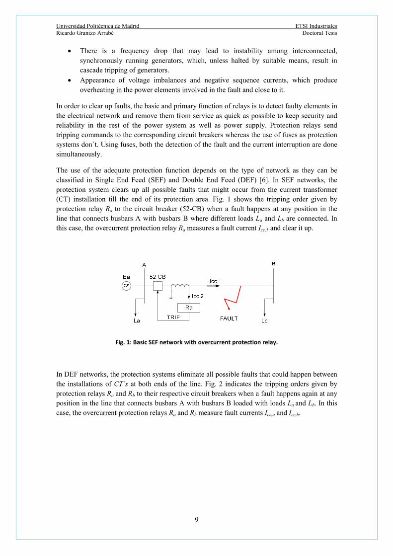
The use of the adequate protection function depends on the type of network as they can be classified in Single End Feed (SEF) and Double End Feed (DEF) [6]. In SEF networks, the protection system clears up all possible faults that might occur from the current transformer (CT) installation till the end of its protection area. Fig. 1 shows the tripping order given by protection relay Ra to the circuit breaker (52-CB) when a fault happens at any position in the line that connects busbars A with busbars B where different loads La and Lb are connected. In this case, the overcurrent protection relay Ra measures a fault current Icc,1 and clear it up.
Fig. 1: Basic SEF network with overcurrent protection relay.
In DEF networks, the protection systems eliminate all possible faults that could happen between the installations of CT´s at both ends of the line. Fig. 2 indicates the tripping orders given by protection relays Ra and Rb to their respective circuit breakers when a fault happens again at any position in the line that connects busbars A with busbars B loaded with loads La and Lb. In this case, the overcurrent protection relays Ra and Rb measure fault currents Icc,a and Icc,b.

Universidad Politécnica de Madrid ETSI Industriales Ricardo Granizo Arrabé Doctoral Tesis
10
Fig. 2: Basic SEF network with overcurrent protection relays.
From Fig. 1 and 2 it has been seen implicitly the protection zone covered by protection relays Ra and Rb. The protection zone is the area of responsibility for the protection system to eliminate faults that arise in such zone as soon as possible. All protection relays generate their own protective zone, normally called “primary protected zone”[7]. Any fault that occurs inside the protective zone, initiates the operation of the protection system. In this case, the fault is known as “internal fault” [8]. However, if a fault takes place outside the protective zone, it does not initiate the operation of the protection relay and the faults is named as “external or through fault”[9].
It is compulsory for a good protection system definition to have at least two protection systems that can clear up faults with different tripping times to ensure that any fault will be eliminated with total security [10]. Therefore, it is normal practise to have a second protection system that could eliminate faults if the first protection system fails. The first protection system is called “primary protection” and the second protection system is named “back-up protection” [11]. The principle of the back-up protection system is that there must be at least a second opportunity to clear up faults. If the primary protection fails to eliminate the fault condition, another protection system should do it and trip its 52-CB associated after the tripping adjusted time at the primary protection system had expired.
Fig. 3: Basic back-up protection system definition.
Universidad Politécnica de Madrid ETSI Industriales Ricardo Granizo Arrabé Doctoral Tesis
11
Fig. 3 explains in an easy way the back-up principle. When a fault happens in line B-C, the first protection system to clear the fault up is the protection relay Rb once the tripping time set has expired as the fault has happened in the protection zone of relay Rb. If this relay Ra fails to eliminate the fault, the back-up protection relay Ra will have to take up the responsibility of eliminating such fault. For this purpose, the protection relay Ra must be set adequately to read the fault current and trip in a longer time than the time adjusted in protection relay Rb, that means that tRa>tRb.
Different causes of primary relaying failure are:
- Failure in CT and/or voltage transformers (VT´s) due to bad design or wrong characteristics that drive them to deliver inadequate current or voltage signals to the protection relays.
- Failure in the leads from CT/VT to the protection relays with wrong connections that can cause bad operation performance in the protection relays.
- Failure of the relay to operate due to inadequate maintenance: moderns protection relays include a “watchdog output contact” that allows having a signal that indicates whether the protection relay is in full operability or not.
- Failure of auxiliary power supply. - Failure in the trip circuit: actual protection relays include the functionality known as
“trip circuit supervision” [12]. Normally the resistance of the tripping coils of the circuit breaker is checked continuously injecting a low value current and measuring the voltage across such tripping coils [13].
- Mistake of the circuit breaker to open, perhaps due to mechanical linkage failure or welded contacts. Those contacts become welded when the circuitbreaker is reclosed on a fault condition [14].
- Wrong settings definition for the protection relays: sometimes the settings introduced in the protection relays are inappropriate and the fault is unable to be eliminated. A proper network and settings coordination studies should be developed to avoid this possibility.
There are two main types of back-up protection systems: Local and Remote. Local back-up has the disadvantage that if there is a failure at the auxiliary power supply, it makes local back up useless unless different auxiliary power supplies are installed. As recommendation it can be said that anything that might make the primary protection system to fail, should not cause the back-up protection system fails too. Remote back-up is normally preferred. Basic considerations must be taken into account for the right implementation of remote back-up protection systems:
- If the operating time for fault clearance of the back-up protection relay is less than the fault duration considered as the setting time adjusted in the primary protection relay plus the operation time of the circuit breaker, the back-up protection relay would trip its corresponding circuitbreaker even with the primary protection relay operating well. In this case there is a complete loss of selectivity.
- The operating time of the back-up protection system must have a time interval higher than the circuitbreaker operating time. Therefore, considering the fault duration indicated previously and a time interval as time of guarantee, the remote back-up protection relay will always operate satisfactorily.

Universidad Politécnica de Madrid ETSI Industriales Ricardo Granizo Arrabé Doctoral Tesis
12
Some examples of coordination of protection relays are indicated subsequently. Fig. 4 shows basic tripping times of back-up protections in a DEF network where protection relays R1 and R3 have directional tripping criteria and only trip when the fault current flows in the right direction. In particular, protection relay R1 trips with currents circulating only from busbars B to busbars C whereas protection relay R3 trips with currents circulating only from busbars B to busbars A. If a fault happens between busbars A and B, the first protection relay to trip is R3 in a time of 0.1 s and then the protection relay R2 would eliminate the fault 0.4 s later. In case that the relay R3 fails to trip, the back-up relay R4 will trip in 0.5 s. The same operation mode is used for faults between busbars B and C. f a fault happens between busbars B and C, the first protection relay to trip is R1 in a time of 0.1 s and then the protection relay R3 would eliminate the fault 0.4 s later. In case that the relay R1 fails to trip, the back-up relay R2 will trip in 0.5 s.
Fig. 4: Basic tripping times of back-up protections in DEF networks.
Fig. 5: Basic tripping times of back-up protections in mesh SEF networks.
Fig. 5 shows the coordination between some protections relays disposed in a SEF mesh network. Protection relays R2, R3, R4 and R5 only trip when the fault currents circulate with the next directions:
- Relay R2: from busbar B to busbar A.

Universidad Politécnica de Madrid ETSI Industriales Ricardo Granizo Arrabé Doctoral Tesis
13
- Relay R3: from busbar B to busbar C.
- Relay R4: from busbar C to busbar B.
- Relay R5: from busbar C to busbar A.
When a fault happens in the line A-B, the first relay to trip must be relay R2 after 0.1 s and then relay R1 after 0.9 s from the beginning of the fault. If relay R2 fails to trip, then relay R4 trips at a time of 0.5 s from the starting of the fault. Also if relay R4 fails to clear the fault, finally relay R6 will trip at 0.9 s from the fault appearance.
For a fault happens in the line B-C, the first relays to trip must be relays R3 and R4 at the same time of 0.5 s. If one of them fails to trip, then relays R1 or R6 will trip at 0.9 s from the fault happened.
Finally, when a fault happens in the line A-C, the first relay to trip must be relay R5 after 0.1 s and then relay R6 after 0.9 s from the beginning of the fault. If relay R5 fails to trip, then relay R3 trips at a time of 0.5 s from the starting of the fault. Also if relay R3 fails to clear the fault, finally relay R1 will trip at 0.9 s from the fault appearance.
Basic overlapping of protection zones has been described and some considerations must always be taken into account when planning a protection coordination study:
- Protected zones not overlapped: in function of the settings introduced in the protection relays, some places of the network might not belong to any protection zone. If a fault occurs in such places, no protection will clear the fault up. Fig. 6 shows a line zone without any protection.
Fig. 6: Protected zones not overlapped.
- Protected zones overlapped but not around protection relays: for a fault at the right side (FAULT 1) of the overlapping area, only protection relay R2 trips. But when the fault is at the left side of the overlapping area, protection relays R1 and R3 trip. However, if the fault happens at the overlapping area, all protection relays R1, R2 and R3 trip.

Universidad Politécnica de Madrid ETSI Industriales Ricardo Granizo Arrabé Doctoral Tesis
14
Fig. 7: Protected zones overlapped.
- Correct overlapping of protective zones around protection relay: this overlapping scheme shows how the protection relay R2 covers also any fault that happens at the protection relay R1.
Fig. 8: Overlapping around protection relay R1.
2.1.1. Methods for ground faults location.
The main methods used for location of ground faults actually are classified in:
- Methods that use the phase information of zero-sequence currents and voltages (Single phase to ground fault location based on phase of zero-sequence current).
- Methods that use the Wavelet Transformation and Travelling Wave Theory (A novel Method for Single Phase to Ground Fault Location Based on Wavelet Analysis and Correlation) and methods that only uses the Travelling Wave Theory.
- Methods that use the post-fault voltages and currents values using DFT (Effective Two Terminal Single Line to Ground Fault Location Algorithm).
Basics of such methods are described following.

Universidad Politécnica de Madrid ETSI Industriales Ricardo Granizo Arrabé Doctoral Tesis
15
2.1.2. Methods that use the phase information of zero sequence currents and voltages
These methods evaluate the phase currents and voltages of the three phases and then they obtain the values of the different sequence components positive, negative and zero. Such methods are implemented in protection relays that have two options to extract the sequence components from the currents and voltage signals:
- Phase currents and voltages inputs are implemented in the protection relay: from those values, the algorithm uses the Fortescue´s Theorem and the components of the three sequences are obtained.
- Zero current and voltage inputs are implemented in the protection relay: in this case there are ring core current transformers installed to measure the zero current or three current transformers using in Holgreem connection. Therefore, only two current inputs are used. Also, there must be three voltage transformers in open-delta connection to obtain the residual voltage. This zero voltage is connected to two inputs in the protection relay.
ANSI codes included in protection relays that use zero components are:
50N and 51N for ground fault overcurrent relays without directional features. 67N for directional ground fault overcurrent relays.
59N for maximum zero voltage.
When the protection relays detect values of zero components over the setting values, they start a timer to give an alarm or tripping command when such timer has expired. The use of these protection systems in distribution or transmission networks allows detecting and clearing ground faults. Their application and use in combined overhead-cable lines is not appropriate to discriminate the position of the ground fault [15] and therefore, the autoreclosing manoeuvre of the combined overhead-cable line might be very risky [16].
ANSI 21 distance protection relays are based in the measuring of the impedance from the fault point to the protection relay. These protection relays use the fundamental frequency of voltage and current signals obtained from measurement elements. The application of distance protection relays is used worldwide due to its easy implementation and low cost at the time of being set up in operation in substations. Two algorithms for distance protection are commonly used depending on the measurements considered [17]:
Only one end terminal data. Two end terminals data.
So far, one terminal data algorithms are used very often in order to develop an accurate and precise estimation of the fault location. This is due to the difficult and limited availability of data exchange between two substation terminals [18].

Universidad Politécnica de Madrid ETSI Industriales Ricardo Granizo Arrabé Doctoral Tesis
16
2.1.3. Methods that use the Wavelet Transformation and Travelling Wave Theory
The use of Wavelet Transformation and Travelling Wave Theory has increased a lot during the last years [19].
The Wavelet transform has shown excellent features to be used as a powerful help for electrical power systems analysis because it can detect a wide range of different events that normally happen at every power network [20], [21]. Thanks to its application, different components of voltages and currents that have high frequencies can be well studied as they have very good temporal resolution while components of those signals that have low frequencies show better frequency resolution.
In order to evaluate changes in voltages and currents as sudden increases or decreases, change in slopes, non-continuities, etc, the Wavelet analysis obtains coefficients with low values if those changes are not big enough. But, if those signals change in a great deal, the coefficients obtained are very high. Also, different singularities or disturbances can be perfectly extracted [22], [23] and [24]. The application of the travelling-wave method is able to extract the high frequency components [25], [26] from voltages or currents that normally appear in transient processes when any type of electrical failure occurs. The fault position in a line with length “l” is calculated considering the time difference, Δt, between the waveforms originated when they reach the specific measuring points. The basics of this theory use the propagation speed of the signal as:
𝜗 =1
√𝐿𝐶 𝑚/𝑠
(1)
L and C are the inductance and capacitance values of the line. Applying the next formula, the fault position is known:
𝑥 =𝑙 − ∆𝑡 · 𝜗
2 𝑚
(2)
Other option to calculate the fault position is to inject a high frequency signal and study its time difference in reaching different measurement points and follow the same process as described before [27].
This method requires at least two different buses in the electrical network to be able to locate the fault. Measurement devices at those buses must be communicated to obtain the time difference of the evaluated signals when they reach such buses.
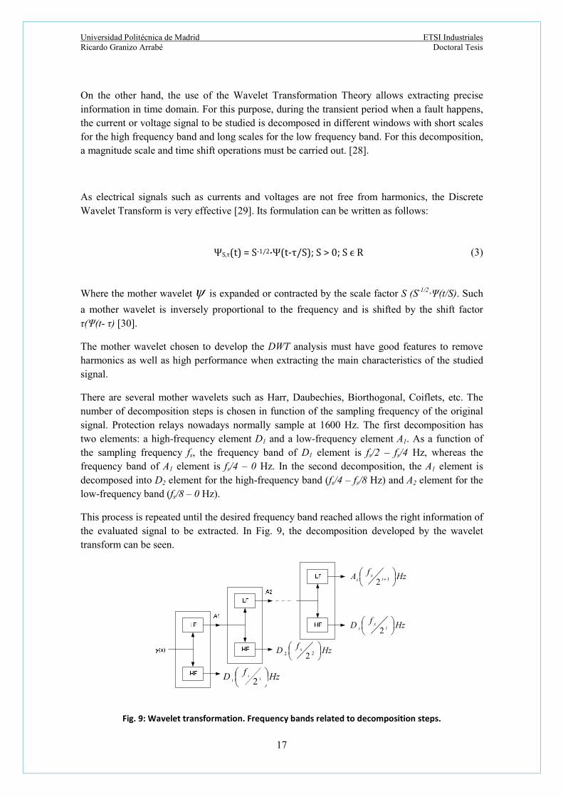
Universidad Politécnica de Madrid ETSI Industriales Ricardo Granizo Arrabé Doctoral Tesis
17
On the other hand, the use of the Wavelet Transformation Theory allows extracting precise information in time domain. For this purpose, during the transient period when a fault happens, the current or voltage signal to be studied is decomposed in different windows with short scales for the high frequency band and long scales for the low frequency band. For this decomposition, a magnitude scale and time shift operations must be carried out. [28].
As electrical signals such as currents and voltages are not free from harmonics, the Discrete Wavelet Transform is very effective [29]. Its formulation can be written as follows:
ΨS,τ(t) = S-1/2·Ψ(t-τ/S); S > 0; S ϵ R (3)
Where the mother wavelet is expanded or contracted by the scale factor S (S-1/2·Ψ(t/S). Such
a mother wavelet is inversely proportional to the frequency and is shifted by the shift factor τ(Ψ(t- τ) [30].
The mother wavelet chosen to develop the DWT analysis must have good features to remove harmonics as well as high performance when extracting the main characteristics of the studied signal.
There are several mother wavelets such as Harr, Daubechies, Biorthogonal, Coiflets, etc. The number of decomposition steps is chosen in function of the sampling frequency of the original signal. Protection relays nowadays normally sample at 1600 Hz. The first decomposition has two elements: a high-frequency element D1 and a low-frequency element A1. As a function of the sampling frequency fs, the frequency band of D1 element is fs/2 – fs/4 Hz, whereas the frequency band of A1 element is fs/4 – 0 Hz. In the second decomposition, the A1 element is decomposed into D2 element for the high-frequency band (fs/4 – fs/8 Hz) and A2 element for the low-frequency band (fs/8 – 0 Hz).
This process is repeated until the desired frequency band reached allows the right information of the evaluated signal to be extracted. In Fig. 9, the decomposition developed by the wavelet transform can be seen.
HzfD is
i
2
HzfD s
22 2
HzfD s
11 2
HzfA is
i
12
Fig. 9: Wavelet transformation. Frequency bands related to decomposition steps.

Universidad Politécnica de Madrid ETSI Industriales Ricardo Granizo Arrabé Doctoral Tesis
18
2.1.4. Methods that use algorithms based on two end terminal measurements The algorithms based on two end terminal measurements improve the typical methods for impedance calculation obtained from one end protection systems. These two end terminal algorithms analyze voltage and current phasors at both ends and therefore, such measurements must be synchronized. Therefore, a communication between both protection systems at both ends must be established.
Two-terminal fault location algorithms have the advantage that a high transmission speed is not necessary to communicate protection systems at both line ends. Typical speed is 57600 Baud [31].
Normally, actual protection relays have a sampling frequency of 1600 Hz and a standard disturbance recorder is included [32]. These disturbance recorders can store voltages and currents during some seconds per disturbance. The pre-fault time can be set for some cycles so the values of voltages and currents magnitudes as well as their phase angles can be known before the fault occurs and during the fault is active till the protection relay sends the corresponding tripping command to clear such fault up.
In general, two terminal algorithms are not influenced neither by the fault resistance nor the knowledge of the Thevenin Equivalent circuits at both line ends.
2.2. Current transformers used in protection systems The application of current transformers together with protection relays demands two different studies that let´s know their performance at steady state and under fault conditions. Unfortunately, it is very common to have current transformers wrongly sized for the application thought and when a failure arises, the protection might work in a bad way and do not clear up the corresponding fault.
Normally all types of responsibilities belong to the protection relays but a good protection engineering must be developed, starting with a good design and sizing of the current transformers to be used.
An easy classification of the transformers used for protection purposes considering the construction forms in function of the voltage level is included as well as some examples to make a good definition of their main features in function of their emplacement in the grid.
The main application of current transformers is to adapt high current values to lower values which are able to be read by measuring equipments and protection relays. Apart from this main feature, current transformers separate primary and secondary windings and therefore exists galvanic isolation. As nominal currents in the secondary side, only two values have been adopted worldwide [33]: 1 and 5 A.
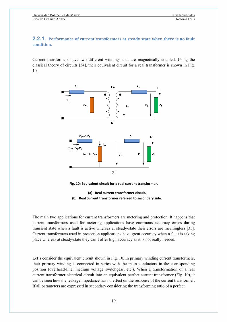
Universidad Politécnica de Madrid ETSI Industriales Ricardo Granizo Arrabé Doctoral Tesis
19
2.2.1. Performance of current transformers at steady state when there is no fault condition.
Current transformers have two different windings that are magnetically coupled. Using the classical theory of circuits [34], their equivalent circuit for a real transformer is shown in Fig. 10.
Fig. 10: Equivalent circuit for a real current transformer.
(a) Real current transformer circuit. (b) Real current transformer referred to secondary side.
The main two applications for current transformers are metering and protection. It happens that current transformers used for metering applications have enormous accuracy errors during transient state when a fault is active whereas at steady-state their errors are meaningless [35]. Current transformers used in protection applications have great accuracy when a fault is taking place whereas at steady-state they can´t offer high accuracy as it is not really needed.
Let´s consider the equivalent circuit shown in Fig. 10. In primary winding current transformers, their primary winding is connected in series with the main conductors in the corresponding position (overhead-line, medium voltage switchgear, etc.). When a transformation of a real current transformer electrical circuit into an equivalent perfect current transformer (Fig. 10), it can be seen how the leakage impedance has no effect on the response of the current transformer. If all parameters are expressed in secondary considering the transforming ratio of a perfect
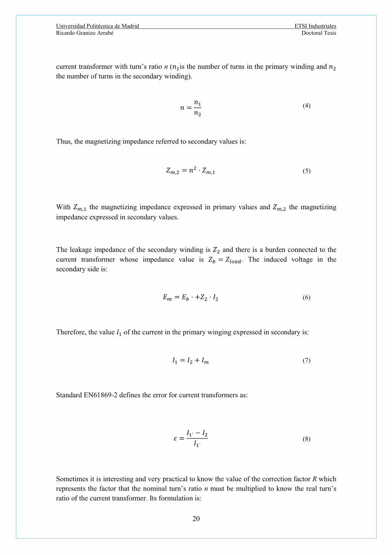
Universidad Politécnica de Madrid ETSI Industriales Ricardo Granizo Arrabé Doctoral Tesis
20
current transformer with turn’s ratio n (𝑛 is the number of turns in the primary winding and 𝑛 the number of turns in the secondary winding).
𝑛 =𝑛
𝑛 (4)
Thus, the magnetizing impedance referred to secondary values is:
𝑍 , = 𝑛 · 𝑍 ,
(5)
With 𝑍 , the magnetizing impedance expressed in primary values and 𝑍 , the magnetizing
impedance expressed in secondary values.
The leakage impedance of the secondary winding is 𝑍 and there is a burden connected to the current transformer whose impedance value is 𝑍 = 𝑍 . The induced voltage in the secondary side is:
Therefore, the value 𝐼 ´of the current in the primary winging expressed in secondary is:
Standard EN61869-2 defines the error for current transformers as:
Sometimes it is interesting and very practical to know the value of the correction factor R which represents the factor that the nominal turn’s ratio n must be multiplied to know the real turn’s ratio of the current transformer. Its formulation is:
𝐸 = 𝐸 · +𝑍 · 𝐼
(6)
𝐼 = 𝐼 + 𝐼
(7)
𝜀 =𝐼 ´ − 𝐼
𝐼 ´
(8)

Universidad Politécnica de Madrid ETSI Industriales Ricardo Granizo Arrabé Doctoral Tesis
21
As the magnetizing impedance is nonlinear, it is necessary to know the correction factor R for interesting working conditions. All current transformers manufacturers provide the excitation curve that represents the secondary voltage in r.m.s. values in function of the excitation current also in r.m.s. values.
2.2.2. Example of calculation of factor R.
This example shows the values of the magnetizing impedance and currents as well as the secondary voltages when in the primary winding there is a circulating current of ten times its rated primary current. Our current transformer has a turn’s ratio of 500/1 A and its excitation curve is shown in Fig. 11.
Fig. 11: Excitation current for 500/1 A current transformer.
The load impedance is 0.8 + 𝑗0.6 Ω and the secondary leakage impedance is considered to have a value of 0.01 + 𝑗0.12 Ω. As the magnetizing impedance is not linear, an equivalent circuit in secondary of the current transformer must be used. First, the primary current of 5000 A (ten times rated current) is represented in secondary using the nominal ratio as 5000 · 1/500 = 10 A. In parallel with this current source there are two impedances connected, one is the total load impedance and the other is the magnetizing impedance. The total load impedance is the sum of the secondary leakage impedance and the load burden. Its value is:
10-4
10-3
10-2
10-1
100
10110
-3
10-2
10-1
100
101
102
Current (A)
Vo
ltag
e (
V)
Excitation curve for CT 500/1 A
𝑅 =1
1 − 𝜀
(9)
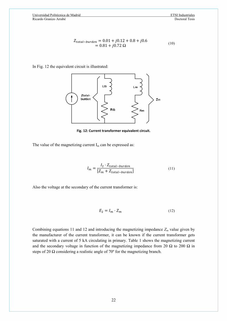
Universidad Politécnica de Madrid ETSI Industriales Ricardo Granizo Arrabé Doctoral Tesis
22
In Fig. 12 the equivalent circuit is illustrated:
Fig. 12: Current transformer equivalent circuit.
The value of the magnetizing current Im can be expressed as:
Also the voltage at the secondary of the current transformer is:
Combining equations 11 and 12 and introducing the magnetizing impedance Zm value given by the manufacturer of the current transformer, it can be known if the current transformer gets saturated with a current of 5 kA circulating in primary. Table 1 shows the magnetizing current and the secondary voltage in function of the magnetizing impedance from 20 Ω to 200 Ω in steps of 20 Ω considering a realistic angle of 70º for the magnetizing branch.
𝑍 = 0.01 + 𝑗0.12 + 0.8 + 𝑗0.6 = 0.81 + 𝑗0.72 Ω
(10)
𝐼 =𝐼 · 𝑍
[𝑍 + 𝑍 ]
(11)
𝐸 = 𝐼 · 𝑍
(12)

Universidad Politécnica de Madrid ETSI Industriales Ricardo Granizo Arrabé Doctoral Tesis
23
Table 1: Magnetizing impedance, current and secondary voltage.
Zm Im E2 Angle Modulus Angle Modulus Angle Modulus
70º
20,00 -31,63 0,47 38,37 9,59 40,00 -32,63 0,25 37,64 9,79 60,00 -32,61 0,16 37,38 9,86 80,00 -32,74 0,12 37,25 9,89
100,00 -32,82 0,09 37,18 9,91 120,00 -32,87 0,08 37,13 9,93 140,00 -32,91 0,07 37,09 9,94 160,00 -32,93 0,06 37,06 9,94 180,00 -32,95 0,05 37,04 9,95 200,00 -32,97 0,05 37,03 9,95
The values included in Table 1 show clearly that the current transformer is not saturated when there are 5 kA circulating in the primary winding. Considering the value of 100 Ω for Zm, the magnetizing current takes up a value of 0,09 A and the current in the burden is 9,91 + 0.053𝑗 A. The error has a value of:
𝜀 = 0,009 , º
And finally the factr R has a value of:
𝑅 = 1,0076 , º
2.2.3. Performance of a current transformer in transients.
When a high current fault takes place, a remarkable DC component has to be considered and probably some remanence might appear. If this is the case, the current transformer could saturate and the secondary current which is driven to protection relays has a high distortion value. It is necessary to establish basic equations considering the relations between the fault current, the burden connected in the secondary of the current transformer and the existing flux in its core when such core has a linear magnetizing curve. Furthermore, as the saturation is not a linear phenomenon, the effects of such nonlinearity must be taken into high consideration. In general terms, when there is a fault, the primary current is defined by the next equation:
𝑖 (𝑡) = 𝐼 · 𝑐𝑜𝑠(𝜔𝑡 − 𝜃) − 𝑒 · 𝑐𝑜𝑠(𝜃)
(13)

Universidad Politécnica de Madrid ETSI Industriales Ricardo Granizo Arrabé Doctoral Tesis
24
Where Ip is the maximum value of the steady-state fault current, T is the time constant of the primary circuit in the power system and θ represents the inception angle when the fault occurs. Fig. 13 shows the equivalent electrical circuit for current transformers used to study the transient analysis where it can be observed the next elements:
Rbb: total resistance of the burden, leakage resistance and cables from the output
terminal in secondary side of the current transformer. Lbb: total inductance of the burden, leakage resistance and cables from the output
terminal in secondary side of the current transformer. Rcc: core resistance.
Lm: magnetizing inductance.
Fig. 13: Equivalent circuit for transient analysis of current transformers. From equation 13, taking the current 𝑖 (𝑡) to Laplace domain and arranging the flux linkage λ as well as the secondary voltage V2 in function of the current I1, and then using the inverse Laplace transformation, the flux linkage λ as well as the secondary current I2 can be expressed as follows:
𝜆(𝑡) = 𝐼 · 𝑐𝑜𝑠(𝜃) ·𝑅 · 𝑅
𝑅 + 𝑅·
𝑒 · −𝜏 · 𝑇
𝜏 − 𝑇+ 𝜏 · (𝑠𝑖𝑛𝜑 · 𝑐𝑜𝑠𝜑 · 𝑡𝑎𝑛𝜃 − 𝑐𝑜𝑠 𝜑)
+𝑒 ·𝜏 · 𝑇
𝜏 − 𝑇+ 𝜏 ·
𝑐𝑜𝑠𝜑
𝑐𝑜𝑠𝜃· 𝑐𝑜𝑠(𝜔𝑡 − 𝜑 − 𝜃)
(14)
𝐼 (𝑡) = 𝐼 · 𝑐𝑜𝑠(𝜃) ·𝑅
𝑅 + 𝑅·
𝑒 · −𝜏 · 𝑇
𝜏 − 𝑇+ (𝑠𝑖𝑛𝜑 · 𝑐𝑜𝑠𝜑 · 𝑡𝑎𝑛𝜃 − 𝑐𝑜𝑠 𝜑)
+𝑒 ·𝜏
𝜏 − 𝑇− 𝜔𝜏 ·
𝑐𝑜𝑠𝜑
𝑐𝑜𝑠𝜃· 𝑠𝑖𝑛(𝜔𝑡 − 𝜑 − 𝜃)
(15)
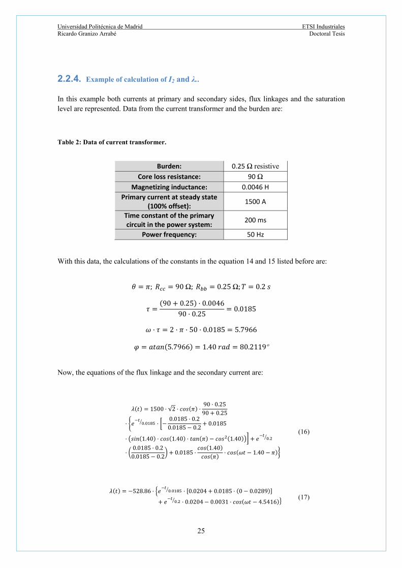
Universidad Politécnica de Madrid ETSI Industriales Ricardo Granizo Arrabé Doctoral Tesis
25
2.2.4. Example of calculation of I2 and λ..
In this example both currents at primary and secondary sides, flux linkages and the saturation level are represented. Data from the current transformer and the burden are:
Table 2: Data of current transformer.
Burden: 0.25 Ω resistive
Core loss resistance: 90 Ω Magnetizing inductance: 0.0046 H
Primary current at steady state (100% offset): 1500 A
Time constant of the primary circuit in the power system: 200 ms
Power frequency: 50 Hz With this data, the calculations of the constants in the equation 14 and 15 listed before are:
𝜃 = 𝜋; 𝑅 = 90 Ω; 𝑅 = 0.25 Ω; 𝑇 = 0.2 𝑠
𝜏 =(90 + 0.25) · 0.0046
90 · 0.25= 0.0185
𝜔 · 𝜏 = 2 · 𝜋 · 50 · 0.0185 = 5.7966
𝜑 = 𝑎𝑡𝑎𝑛(5.7966) = 1.40 𝑟𝑎𝑑 = 80.2119º
Now, the equations of the flux linkage and the secondary current are:
𝜆(𝑡) = 1500 · √2 · 𝑐𝑜𝑠(𝜋) ·90 · 0.25
90 + 0.25
· 𝑒 . · −0.0185 · 0.2
0.0185 − 0.2+ 0.0185
· 𝑠𝑖𝑛(1.40) · 𝑐𝑜𝑠(1.40) · 𝑡𝑎𝑛(𝜋) − 𝑐𝑜𝑠 (1.40) + 𝑒 .
·0.0185 · 0.2
0.0185 − 0.2+ 0.0185 ·
𝑐𝑜𝑠(1.40)
𝑐𝑜𝑠(𝜋)· 𝑐𝑜𝑠(𝜔𝑡 − 1.40 − 𝜋)
(16)
𝜆(𝑡) = −528.86 · 𝑒 . · [0.0204 + 0.0185 · (0 − 0.0289)]
+ 𝑒 . · 0.0204 − 0.0031 · 𝑐𝑜𝑠(𝜔𝑡 − 4.5416)
(17)
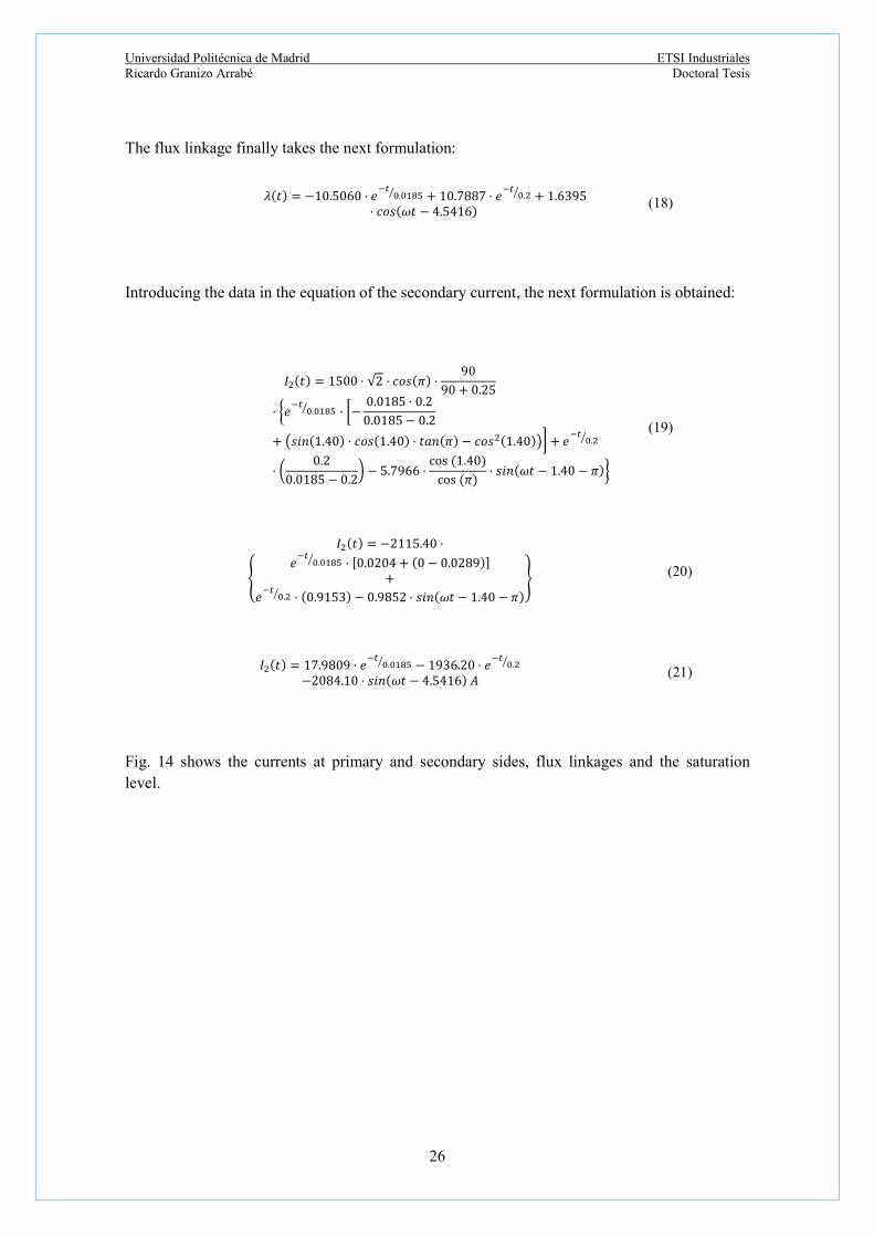
Universidad Politécnica de Madrid ETSI Industriales Ricardo Granizo Arrabé Doctoral Tesis
26
The flux linkage finally takes the next formulation:
Introducing the data in the equation of the secondary current, the next formulation is obtained:
Fig. 14 shows the currents at primary and secondary sides, flux linkages and the saturation level.
𝜆(𝑡) = −10.5060 · 𝑒 . + 10.7887 · 𝑒 . + 1.6395· 𝑐𝑜𝑠(𝜔𝑡 − 4.5416)
(18)
𝐼 (𝑡) = 1500 · √2 · 𝑐𝑜𝑠(𝜋) ·90
90 + 0.25
· 𝑒 . · −0.0185 · 0.2
0.0185 − 0.2
+ 𝑠𝑖𝑛(1.40) · 𝑐𝑜𝑠(1.40) · 𝑡𝑎𝑛(𝜋) − 𝑐𝑜𝑠 (1.40) + 𝑒 .
·0.2
0.0185 − 0.2− 5.7966 ·
cos (1.40)
cos (𝜋)· 𝑠𝑖𝑛(𝜔𝑡 − 1.40 − 𝜋)
(19)
𝐼 (𝑡) = −2115.40 ·
𝑒 . · [0.0204 + (0 − 0.0289)]+
𝑒 . · (0.9153) − 0.9852 · 𝑠𝑖𝑛(𝜔𝑡 − 1.40 − 𝜋)
(20)
𝐼 (𝑡) = 17.9809 · 𝑒 . − 1936.20 · 𝑒 . −2084.10 · 𝑠𝑖𝑛(𝜔𝑡 − 4.5416) 𝐴
(21)

Universidad Politécnica de Madrid ETSI Industriales Ricardo Granizo Arrabé Doctoral Tesis
27
Fig. 14: Currents I1, I2, 𝝀 and saturation level.
When the flux linkages 𝜆 have values over the saturation level, the secondary current will turn out to be close to zero. Therefore, the time response of the flux linkages 𝜆 is responsible of the core saturation of the current transformer. That means that, apart from the class of the current transformer, the secondary current is not representing perfectly the primary current. If this situation happens, the protection relays connected to such current transformer might have severe difficulties to operate correctly and develop unintended tripping commands. When a protection system is being developed, it must be paid high attention to the definition of the features of current transformers in order to avoid their saturation under any working condition.
2.2.5. Connections of current transformers for detecting ground fault currents.
The first thing to be known before choosing an specific connection of current transformers for detecting ground fault currents is precisely to know the possible values of those ground fault currents. A power flow and short-circuit analysis must be carried out previously.
The values of the ground fault currents obtained in function of the grounding method applied will let´s know the ratings of the current transformers to be implemented as well as their connections. Table 3 indicates the main characteristics of ground fault currents for different grounding systems:
For solidly grounded power systems, ground faults can be detected using the residual current circuit known as Holmgreen Circuit. Its connection is shown in Fig. 15 [36].
0 0.1 0.2 0.3 0.4 0.5 0.6 0.7 0.8 0.9 1-3000
-2000
-1000
0
1000
2000
3000
4000
5000
Time (s)
Am
pere
s -
We
ber
Flux linkages, primary and secondary currents
Flux linkagesSecondary current I2Primary current I1Saturation level
Saturationzone for I2

Universidad Politécnica de Madrid ETSI Industriales Ricardo Granizo Arrabé Doctoral Tesis
28
Table 3: Main characteristics of ground faults.
Characteristics of ground
faults
Solidly Grounded
Grounding by
Impedance Ungrounded
Ground fault current
High Wide range Low
Fault detection Easy Easy Not so easy
Selectivity Easy Easy Difficult
Fig. 15: Holmgreen Circuit.
The secondary windings of the three current transformers are connected in parallel after leaving the current inputs I1, I2 and I3 of the three phases in the protection relay. Therefore, the neutral current input IE in the protection relay is always measuring the residual current as follows:
This way, when a ground fault happens and the current value in at least one phase is too high, the current input for ground currents Ie is measuring such value and the ground fault is detected.
𝐼 + 𝐼 + 𝐼 = 3𝐼
(22

Universidad Politécnica de Madrid ETSI Industriales Ricardo Granizo Arrabé Doctoral Tesis
29
As the protection relays installed nowadays normally have as minimum setting for ground fault protection 1% [37] of the nominal current transformer, the sensibility is more than enough.
In power systems with impedance grounding or ungrounded, it is common practice to install a ring core current transformer and pass the cables of the three phases through it. The correct way of installation of such ring core current transformer is passing the three phases through its internal hole including the shields. The junction of the shields done outside the ring core current transformer must be passed again through the ring core current transformer as indicated in Fig. 16, [38].
Let´s consider resistive loads in the three phases and the given phase currents as follows:
The ring core current transformer will deliver to the ammeter connected to its secondary terminals a current of:
Fig. 16: Correct grounding connection of shields.
𝐼𝐼𝐼
=
15 º
30 º
45 º
𝐴
(23)
𝐼 + 𝐼 + 𝐼 = · (15 º + 30 º + 45 º) = 0.5196 º A
(24)

Universidad Politécnica de Madrid ETSI Industriales Ricardo Granizo Arrabé Doctoral Tesis
30
A wrong grounding of the common shield not through the internal hole of the ring core current transformer is indicated in Fig. 17.
Fig. 17: Incorrect grounding connection of shields.
In this case, the results are:
With this easy example, the grounding of shields must be perfectly arranged. Otherwise the currents given to the protection relays might drive them to send wrong tripping orders. As it has been explained, a correct grounding of the shields is a must for any protection system that had to clear ground faults. No mistakes in the ground connections of the shields are allowed because it is a key factor to let the protection systems discriminate where the ground fault has taken place.
𝐼 + 𝐼 − 𝐼 + 𝐼 = · (15 º + 45 º) = 0.7937 . º A
(25)

Universidad Politécnica de Madrid ETSI Industriales Ricardo Granizo Arrabé Doctoral Tesis
31
2.3. Grounding systems of power cable shields.
The main systems used for grounding the shields of power cables are described. First, a brief explication deals with the development of currents along the shields. Then, the advantages and disadvantages of the grounding systems used are includedof how currents in shields are developed. Finally, the selection of protections against overvoltages is included.
2.3.1. Introduction.
When the grounding connections of the shields in power cables are studied, it must be taken in high consideration the fact that the conductor and its screen form a very strong magnetically coupled system owing to the magnetic field generated in the conductor when there is current circulating through it.
Therefore, when a circulating current in the conductor changes its value along a period of time, the varying magnetic field is also variable and is developed in the space surrounding the conductor. Following the law of Ampere-Maxwell [39], there is an equation that relates circulating currents and the corresponding magnetic field created. This equation is:
𝑟𝑜𝑡 = 𝐽 +𝜕𝐷
𝜕𝑡 (26)
It can also be expressed as follows:
. 𝑑𝑙 = 𝐽. 𝑑𝑆 +𝜕𝐷
𝜕𝑡. 𝑑𝑆 = 𝑁𝐼 + 𝐼 (27)
The term Id is called displacement current and appears only when there are varying electric fields. So that the faster varying the electric field the greater will be the displacement current. Therefore, the contribution of the total displacement current to the magnetic field is proportional to its value. However, in electrical power systems as transmission or distribution power networks, the displacement currents are in general much lower than the currents circulating through the conductors [40]. This way, their contribution to the total magnetic field is much reduced and this current can usually be neglected.
If the term Id is not considered, equation (27) can be understood in the way that any circulation of any magnetic field on a closed path is equal to the total current which goes through the corresponding curved surface. In particular, the magnetic field intensity can be related to the

Universidad Politécnica de Madrid ETSI Industriales Ricardo Granizo Arrabé Doctoral Tesis
32
magnetic induction which considers the magnetic permeability of the medium, using the next expression:
𝐵 = 𝜇 (28)
The magnetic field created has an asoccitaed magnetig flux and considering a specific surface A which belongs to the shields and is perpendicular to the magnetic field force lines, the magnetic flux through such surface A is determined by:
∅ = 𝐵. 𝑑𝐴 (29)
As the currents circulating in power cables are variable in time, the magnetic fluxes obtained will also be variables in time. Following Faraday-Lenz equation [41], when a variable magnetic flux in time goes across any surface, an electromotive force is induced in the contour of such surface. Its formulation is:
. 𝑑𝑙 = −𝜕
𝜕𝑡𝐵. 𝑑𝐴 ⟹ 𝑢 = −
𝜕∅
𝜕𝑡 (30)
If in the contour of the surface taken into account does exist a conductor circuit as in the case of shields in power cables, owing to the action of a magnetic field variable in time, an induced voltage will appear in those shields. Fig. 18 shows the force lines of the magnetic field caused by the circulation of current through the main conductor.
Fig. 18: Magnetic field created by an electrical current.

Universidad Politécnica de Madrid ETSI Industriales Ricardo Granizo Arrabé Doctoral Tesis
33
As there is an induced voltage over a conductor named shield, there will appear an induced current in such shield whose direction following Lenz Law will be in the way that its corresponfding flux opposes to the inductor flux. There are two different types of current induced related directly to the form of grounding the shields:
Circulating currents [41], [42]: They are obtained when the shields are grounded at both
ends. A closed circuit is formed by the shields and the ground return path. In this case, the induced current circulates along this closed circuit and is responsible of power losses due to the resistance of the shields.
Fig. 19: Circulating currents induced in shields.
Eddy or Foucault currents [43]: such currents are obtained when the shields are grounded only in one end and a close circuit is not formed. In such conditions, the induced currents only circulate across the volume of the shields and dissipate energy in terms of heat.
Fig. 20: Induced Foucoult currents in shields.

Universidad Politécnica de Madrid ETSI Industriales Ricardo Granizo Arrabé Doctoral Tesis
34
When the shields are grounded at their ends, both induced currents are created. However, the effects of eddy currents are much reduced compared to the effect caused by the circulating currents in the shields. In any case, if there are not circulating currents, the efffect of eddy currents can´t be forgotten as it creates losses in the power cables.
Due to the effect of the electromagnetic induction, induced voltages appear in the shields and, in function of the connections of those shields, circulating currents might exist or not [44]. Such effects are created in:
Steady state.
Shortcircuit.
o During the transient time. o In permanent shortcircuit regime.
Fig. 21 shows currents induced in a closed circuit form by shields of a two-phase system.
Fig. 21: Induced currents in shields.
The circulation of currents through the shields of power cables is created by the connection of them and not because their grounding. Such curents are related to the wiring configuration and the coefficients of mutual induction between conductors and shields, which are based on the type of cable and the separation between them. Those coeefficients of mutual induction depends on the type of power canle and the distance between them.
Universidad Politécnica de Madrid ETSI Industriales Ricardo Granizo Arrabé Doctoral Tesis
35
Because of contact voltage values, the connection points of shields are grounded and two types of connections are used:
Grounding of only one end of the shields: a close circuit is not stablished and
circulating currents are unable to flow. However, induced voltages are developed and can become very dangerous at the non grounded end, mainly for the cover of the cacle.
Connection of both ends of the shields: now a clsed circuit is formed and circulating currents flow. These currents increase the losses of the cable and become a thermal problem for the isolating of the cable. Furthermore, their circulation reduces the power capacity to be transmitted by these power cables.
Following the described before, the challenges of a proper design of grounding systems for shield connections are the security of persons and electrical equipments and the next considerations must be taken into high consideration:
Elimination or high reduction of circulating currents at steady state due to the inductive
coupling with the main stream current in the conductors. This reduction will reduce the losses of active power [45].
Reduction at both steady state and shortcircuit regime, of the induced voltages between
shields of power cables and ground. During shortcircuits, those induced overvoltages might perforate the insulation of the cover or create important discharges at the connections boxes of shields where shield transpositions are done [46].
At steady state, the capacitive currents must be driven to ground.
During lighning strokes and overvoltages caused by switching operations, there should be specific devices that limit the values of those overvoltages to avoid the perforation of the covers [47].
The next types of grounding methods for shields are normally used [48]:
Both ends grounded: this type of grounding is known as Solid-Bonding. Only one end grounded: this type of grounding is known as Single-Point. Transposition of shields: this type of grounding is known as Cross-Bonding. Transposition of conductors and shields.
These types of grounding methods for shields are described then [49].
2.3.2. Grounding of both ends of the shields. Solid-Bonding (SB).
In this method, both ends of the shields are grounded. In order to not overcome the voltages that the covers can withstand in long lines with high shortcircuit current values, it is desirable that the shields connections along the cable are also grounded.

Universidad Politécnica de Madrid ETSI Industriales Ricardo Granizo Arrabé Doctoral Tesis
36
This system is applicable in medium voltage lines generally with short length. In these cases, it can be stimated that the power losses in the shields reduce the nominal current of the line between 10% and 25% in medium voltage, and up to 50% in high voltage lines. When the currents flowing through the conductors of the cables are high, in the range of 500A or higher values, the losses turn out to be high and other grounding methods for shields are used [50].
Benefits of this method:
In steady state, the voltage between the screen and ground along the line is close to
zero. This difference of potential is only due to the circulation of the capacitive currents of the cable.
In steady state, the contact voltage at the ends of the screens is zero for a staggered distribution cable, and generally small for a layer or flag under non-symmetrical distribution. For non-symmetrical arrangements, cable can be transposed, both conductors and their screens. This way, it is possible to reduce losses and the contact voltage at the ends of the screens.
Both arrangements layer and staggered, if there is an asymmetrical fault not in the cable, a voltage will be induced owing to the coupling between the conductor and the screen, and therefore a current will circulate along the screen and flow at the grounding at both ends. The circulation of current along the screens reduces the induced voltage across them.
It is the simplest connection system for screens; it does not require any accessories and screens are grounded in an easy way.
Drawbacks of this method:
There is power loss when there is a current circulating in the screens. As the circuit is closed, the voltage induced on the screens turns out to be in a current circulation. Thus by increasing the losses in the cable, the capacity for power transmission is decreased. This is the reason why, except for medium-voltage or short distances of a few kilometers, other forms for screen connection are used.
Installation conditions:
In order to reduce the induced voltage, and therefore circulating currents, cables must be arranged in triangle, or staggered.
If the installation system has a flat or layer disposal by transposing cables, equal currents through the corresponding screen circulate and therefore there is less power losses compared to cables without transposition. But in any case, transposition does not eliminate currents in the screens.

Universidad Politécnica de Madrid ETSI Industriales Ricardo Granizo Arrabé Doctoral Tesis
37
The following figures show typical connection diagrams for shields at their two ends or solid-bonding:
Fig. 22: Solid-bonding arrangement (SB).
Fig. 23: Solid-bonding arrangement (SB) with intermediate joint.
Fig. 24: Solid-bonding arrangement (SB) with transposition of conductors.

Universidad Politécnica de Madrid ETSI Industriales Ricardo Granizo Arrabé Doctoral Tesis
38
For the simplest scheme shown in Fig. 25, the approximate profiles of induced voltages are shown below:
Fig. 25: Induced voltage in solid-bonding arrangement (SB).
As it can be observed, the highest induced voltage occurs in the middle of the line, but generally is not very high. Moreover, it is also seen that induced voltages are zero at the ends of the screen as they are rigidly grounded. Such induced voltages may be different from zero if there is any current flowing through the grounding of the screens. This circumstance happens for example in a layer arrangement.
2.3.3. Grounding at only one end of the shields. Single-Point (SP) or Mid-Point (MP).
In single point (SP) connection system for screens, such screens are grounded at one end of the line. The other end of the screen is isolated from ground through the outer cover [51], [52].
In a similar way, in the mid point (MP) connection system for screens, they are grounded in an intermediate joint whereas the screens at their two ends of the line are isolated from ground also through the outer cover.

Universidad Politécnica de Madrid ETSI Industriales Ricardo Granizo Arrabé Doctoral Tesis
39
Both systems have the advantage of not presenting a current circulation through the screens as their circuit is not closed. Therefore the losses that occur are due exclusively to Foucault losses or eddy losses, or eddy currents, which are considerably smaller. Consequently, both methods are used in lines with a total length that allows performing the laying on one, or at most two sections. SP is normally used for short lengths and MP for longer stretches, requiring an intermediate joint. The SP system is usually applied in cables with rated voltage equal or higher than 26/45 kV and not very long in the range from 500 to 600 m. It is common to use in one or both ends of a line of great length with cross- bonding (CB) method when it is impossible to complete the sequence of three sections of equal length and remains a stretch to complete.
For the same value of induced voltage in steady state at the end of the screen not grounded, the MP arrangement can cover twice the length of the SP method, since both screens are earthed in the middle of the length of the cable, leaving two ends ungrounded.
Advantages of the system:
There aren´t power losses on the screens due to circulating currents, except the losses
regarding the Foucault currents. They always exist but can be considered almost negligible.
Drawbacks of the system:
There is an induced voltage in steady state at the end of the non-grounded screens, being this point where it reaches its maximum value. Therefore, at this point the critical voltage of the outer cover can be overcome and have a perforation. This induced voltage has values close to 6 kV at rated frequency and 20 kV at switching. Therefore the lengths of the cables that employ this system should be small.
In transient regime, such as short circuit, the voltage induced at the ends of the screens which are ungrounded presents very high values [53]. Since it would be very expensive to use an outer cover that could withstand those electrical stresses, surge arresters or screen voltage limiters (LTP) are commonly used, which drain the fault current through the screens. This device increases the final cost of the installation, so it is used in short lengths of underground lines when losses are the key factor in it. The type of surge arrester to be installed depends on the length of the strecht. If the end which is not directly grounded is accessible (transitions overhead-cable or terminals of switchgears in substations), the screen-surge arrespeter assembly must be conveniently protected by a plastic case and insulation taping because it is a point in permanent service with voltage.
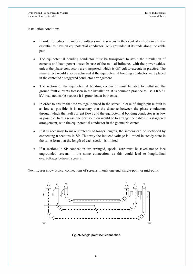
Universidad Politécnica de Madrid ETSI Industriales Ricardo Granizo Arrabé Doctoral Tesis
40
Installation conditions:
In order to reduce the induced voltages on the screens in the event of a short circuit, it is
essential to have an equipotential conductor (ecc) grounded at its ends along the cable path.
The equipotential bonding conductor must be transposed to avoid the circulation of currents and have power losses bacuse of the mutual influence with the power cables, unless the phase conductors are transposed, which is difficult to execute in practice. The same effect would also be achieved if the equipotential bonding conductor were placed in the center of a staggered conductor arrangement.
The section of the equipotential bonding conductor must be able to withstand the ground fault currents foreseen in the installation. It is common practice to use a 0.6 / 1 kV insulated cable because it is grounded at both ends.
In order to ensure that the voltage induced in the screen in case of single-phase fault is as low as possible, it is necessary that the distance between the phase conductors through which the fault current flows and the equipotential bonding conductor is as low as possible. In this sense, the best solution would be to arrange the cables in a staggered arrangement, with the equipotential conductor in the geometric center.
If it is necessary to make stretches of longer lengths, the screens can be sectioned by connecting n sections in SP. This way the induced voltage is limited in steady state in the same form that the length of each section is limited.
If n sections in SP connection are arranged, special care must be taken not to face ungrounded screens in the same connection, as this could lead to longitudinal overvoltages between screens.
Next figures show typical connections of screens in only one end, single-point or mid-point:
Fig. 26: Single-point (SP) connection.

Universidad Politécnica de Madrid ETSI Industriales Ricardo Granizo Arrabé Doctoral Tesis
41
Fig. 27: Mid-point (MP) connection.
Fig. 28: Shields with n stretch in SP connection concatenated. In the case of the simplest scheme shown in Fig. 29, the approximate profiles of the induced voltages are as follows:

Universidad Politécnica de Madrid ETSI Industriales Ricardo Granizo Arrabé Doctoral Tesis
42
Fig. 29: Induced voltage in single-point (SP) connection.
Observing the previous figure, LTPs are placed in the open end of the screen, where the highest induced voltages occur. Therefore it is a must in the protection of the cover to know the values of the induced voltages seen by the LTP (local voltages) and the voltages seen by the covers (absolute voltages). The following figure shows in greater detail both voltages:
Fig. 30: Local and absolute voltages in a SP system.
Depending on the situation and connection of the LTPs, these will act according to the local voltage (does not consider the voltage drop that can occur in R22), while the covers are subject to

Universidad Politécnica de Madrid ETSI Industriales Ricardo Granizo Arrabé Doctoral Tesis
43
the absolute voltage. This situation requires a correct selection of the LTP to ensure that they act before the drilling of the covers [54], [55].
On the other hand, there are two types of protection against transient overvoltages that are usually used for cable protection. These types are:
• Lightning arresters or auto-valves. These devices are designed and prepared to limit
transient overvoltages that may eventually appear on the network and that in the absence of adequate protection, may compromise the insulation of the elements connected to it. They are therefore used in the protection of equipment such as power transformers, cables, etc. They are always used for the protection of the insulation of the cable, being their habitual use in transitions overhead to cable. Such transitions overhead to cable are especially sensible zones where overvoltages can appear due to the change in the characteristic impedance that always takes place in those transitions.
Lightning arresters or auto-valves are used in the protection of cables independently of the grounding system of the screens. This means that such protection devices are used in systems with SB, SP, MP and CB shield connections.
• Shield voltage limiters. These elements are destined to protect the covers of the cables as they limit the transient surges that could arise.
They are used both in SP and MP systems (in the open end of the screen circuit), and in CB systems (at the transposition connections of the screens).
In general, the principle of operation of both devices is the same, as the two types are constituted by non-linear variable resistors. However each device will present certain particular characteristics adapted for the protection of the element for which it is intended to be used. The following figure it is shown the emplacement of both types of devices in an overhead-ground transition, with a configuration of the output cables in SP. Despite the arrangement seen in the figure, it is common use to dispose the grounded end as close as possible to the entry of transient overvoltages.

Universidad Politécnica de Madrid ETSI Industriales Ricardo Granizo Arrabé Doctoral Tesis
44
Fig. 31: Surge-arrester and LTP emplacements in cable with SP connection.
2.3.4. Cross-bonding connection (CB).
The CB shield connection system consists of dividing the line into three equivalent lengths by installing longitudinally insulated splices against the ground and crossing the shields at each splice. Since the phase conductors are arranged geometrically always in the same position when transposing the screens, the voltages induced in them in the three sections will be identical but with a phase shift of 120 °. Under such working conditions, their vector sum is zero and there will be no circulation of currents in the screens.
Therefore the cable screens will be interrupted and transposed in an orderly way taking advantage of the cable connection points. To achieve this, a deep study of the line layout, the number of splices and their situation must be developed in order to have a number of sections multiple of three, keeping the lengths of the sections practically equal.
It is the most recommended method for large lengths and rated voltages greater than or equal to 26/45 kV, and therefore it is the most used method in long high voltage lines.
Benefits of the system:
For a staggered conductor arrangement, the steady-state induced voltage with balanced
loads in three consecutive sections of screens is zero, since it is the sum of three equal voltages which have 120º differences. The mutual inductances between conductors and

Universidad Politécnica de Madrid ETSI Industriales Ricardo Granizo Arrabé Doctoral Tesis
45
screens are equal in the three phases. Consequently, there are neither circulation currents in the screens nor any associated loss.
For an arrangement of conductors in layer or flag disposal, the voltage induced in steady state with loads balanced in three consecutive sections of shields, is reduced, but not zero, since the mutual inductances between conductors and screens are equal in the three phases. Therefore, there will be a permanent current circulation through the ground at the ends. However, although the circulation currents in the shields are not zero, they are small compared to other connections such as SB.
With respect to the connection in SP, the CB in steady mode with staggered cables achieves a zero voltage between screen and earth at both ends and small for CB with cables in layer or flag disposal, as the small asymmetry in the arrangement of cables. It produces a current circulation through the grounding, being different from zero the sum of the three currents in the shields.
The maximum voltage between shields and ground in a CB system will be three times lower than for an arrangement of the same length in SP connection. These maximum voltages occur at the transposition points of the screens.
Due to the effect of magnetic field compensation by the current that circulates in the screens, the induced voltages in case of short circuit on other cables erected in parallel are smaller than for an arrangement in SP connection.
It is not necessary to install an equipotential conductor ecc.
Disadvantages of the system:
At the points where the transposition of the screens is carried out, connection boxes
provided with voltage limiters (LTP) must be installed to control the overvoltages between screens and screen-ground. In this situation, the local voltage coincides with the absolute voltage since there is usually no current flowing through the earthings of the arresters.
Installation conditions:
The three sections that make up a CB system must be approximately of the same length,
having a limit for each section of the order of 500 or 600m. The end of each section, where the transposition of screens is performed, is matched with the splices.
For installations of large lengths where it is difficult to ensure that the number of cable lengths is a multiple of three, this arrangement is combined with one or two final sections in SP conenction.
In function of how the length of the line is divided, there are two options: Sectional Cross-Bonding, or Continuous.
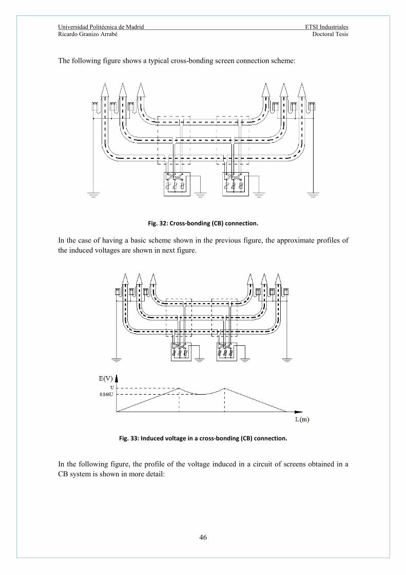
Universidad Politécnica de Madrid ETSI Industriales Ricardo Granizo Arrabé Doctoral Tesis
46
The following figure shows a typical cross-bonding screen connection scheme:
Fig. 32: Cross-bonding (CB) connection.
In the case of having a basic scheme shown in the previous figure, the approximate profiles of the induced voltages are shown in next figure.
Fig. 33: Induced voltage in a cross-bonding (CB) connection. In the following figure, the profile of the voltage induced in a circuit of screens obtained in a CB system is shown in more detail:
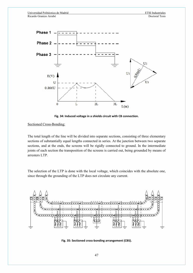
Universidad Politécnica de Madrid ETSI Industriales Ricardo Granizo Arrabé Doctoral Tesis
47
Fig. 34: Induced voltage in a shields circuit with CB connection. Sectioned Cross-Bonding:
The total length of the line will be divided into separate sections, consisting of three elementary sections of substantially equal lengths connected in series. At the junction between two separate sections, and at the ends, the screens will be rigidly connected to ground. In the intermediate joints of each section the transposition of the screens is carried out, being grounded by means of arresters LTP.
The selection of the LTP is done with the local voltage, which coincides with the absolute one, since through the grounding of the LTP does not circulate any current.
Fig. 35: Sectioned cross-bonding arrangement (CBS).

Universidad Politécnica de Madrid ETSI Industriales Ricardo Granizo Arrabé Doctoral Tesis
48
Continuous Cross-Bonding:
In this case only the screens at the ends of the line will be rigidly grounded. At the intermediate joints of each section and at the junction between two sections, the grounding will be done through arresters.
This will be the preferred connection since it allows controlling the display current, whatever the number of sections, by measuring it at one of its ends. It also allows the control of the insulation of the cover and the arresters, opening the connections of the ends and measuring from one of them [56]. In addition, in the case of sectioned cross-bonding, the lengths in all sections must be equivalent, In this case there may be greater margin balancing the length in another section, and may not even be a multiple of three the number of sections.
However, in this case, the transient voltages are generally higher than in the cross-bonding sectioned because there are no intermediate points grounded.
Fig. 36: Continuous cross-bonding (CCB) connection.
2.3.5. Transposition of conductors and shields.
The system of connection of screens by means of transposition of conductors and screens, manages to cancel the circulation of currents for any arrangement of non-symmetrical conductors, such as layer or flag. Its use does not make sense for staggered conductors, since the same effect is achieved with a CB system, which is simpler [57].
Advantages of the system:
The induced voltage along a screens circuit is zero, since in each of the three sections
the induced voltages are equal, and they are offset 120º from each other. This is accomplished as long as the three lengths are of the same length, and the separation

Universidad Politécnica de Madrid ETSI Industriales Ricardo Granizo Arrabé Doctoral Tesis
49
between conductors is maintained. Therefore, the power lost by circulation of currents is zero, as is an SP arrangement.
Regarding the arrangement in SP connection, the induced voltages between screens, and between screen and ground, in both permanent and transient modes, are reduced.
When transposing conductors, as it is done in overhead lines, the line voltage drops are the same in each phase. Consequently, at the end of the line there is a balanced three-phase voltage system.
Drawbacks of the system:
There is a high difficulty of practical execution in the installation. This is why the CB
connection solution is usually used in a staggered system, which provides the same advantages and is simpler.
Fig. 37: Transposition of conductors and shields.
2.3.6. Selection of voltage limiters on shields.
SP, MP and CB connection systems have as main advantage the reduction or elimination of circulation of currents, but they have the disadvantage that the overvoltages that appear during the short circuits are much greater than for the SB system. Therefore it is necessary to use surge protections, normally called varistors or LTP (screen voltage limiters), whose function is to protect the insulation of the covers, as well as the splices and boxes where the transposition of screens is done [58], [59], [60].
Some of the main considerations to take into account in the selection of LTP´s are:

Universidad Politécnica de Madrid ETSI Industriales Ricardo Granizo Arrabé Doctoral Tesis
50
Both the rated voltage of the LTP, Ur, and the voltage supported by the cover at
industrial frequency, Ufw, must be greater than the temporary overvoltage between screens and ground that may occur in the event of a short circuit.
The temporary overvoltage between screen and ground in the event of a short circuit is that which occurs after the initial transient, until the shortcircuit is eliminated, and therefore has a characteristic frequency of 50 Hz.
The value of this overvoltage does not depend on the highest voltage in the network, but on the short-circuit current, the short-circuit type (single phase, two-phase or three-phase), the length of the elementary sections in the arrangement CB or SP, the type of fault, according to whether the cable is installed between substations or in siphon arrangements, and the separation and distribution of conductors (layer, staggered, in contact or under pipe).
To verify if the rated voltage of the LTP and the voltage at industrial frequency supported by the cover are greater than the temporary overvoltage that may appear in the event of a short circuit, it is necessary to calculate it. The overvoltage is calculated as the product of the voltage that appears between the screen and ground by short-circuit ampere multiplied by the short-circuit current. The values of the screen-ground voltages per ampere can not be determined by simple analytical formulation, but are obtained by means of numerical calculation programs, or alternatively by summary tables, obtained by applying the programs for the different scenarios. In the particular case of CB connection, at the transposition points should also be studied the overvoltages between screens.
For the above calculation, it should be noted that the screen-ground voltage increases with the length of the section studied non- in allinear way, as it strongly depends on the values of the grounding resistances at the ends of the section.
The LTPs selected for each grid voltage level must guarantee, for lightning-type impulses, a protection margin equal to or greater than 100% of the level of insulation supported by the cover, splices, or transposer boxes of screens against lightning-type impulses.
The margin of protection in (%) is defined as:
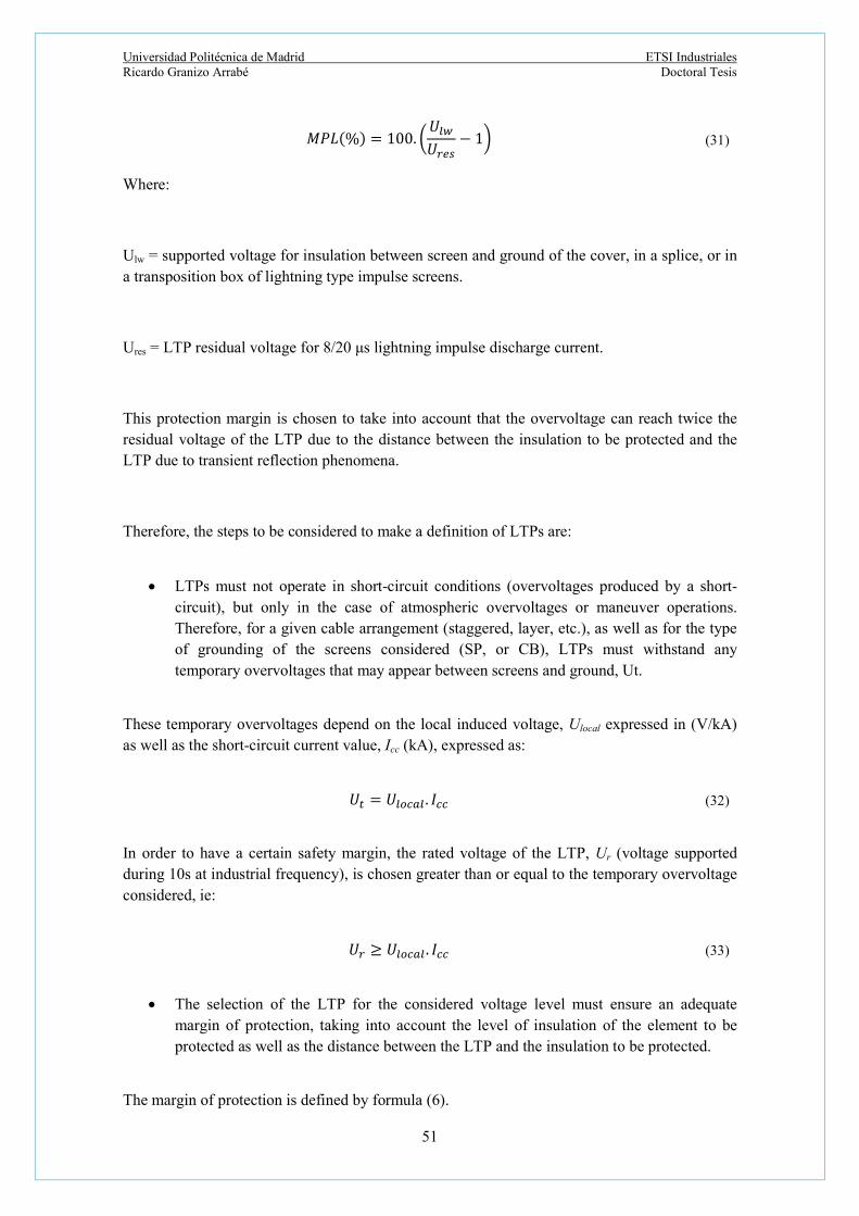
Universidad Politécnica de Madrid ETSI Industriales Ricardo Granizo Arrabé Doctoral Tesis
51
𝑀𝑃𝐿(%) = 100.𝑈
𝑈− 1 (31)
Where:
Ulw = supported voltage for insulation between screen and ground of the cover, in a splice, or in a transposition box of lightning type impulse screens.
Ures = LTP residual voltage for 8/20 μs lightning impulse discharge current.
This protection margin is chosen to take into account that the overvoltage can reach twice the residual voltage of the LTP due to the distance between the insulation to be protected and the LTP due to transient reflection phenomena.
Therefore, the steps to be considered to make a definition of LTPs are:
LTPs must not operate in short-circuit conditions (overvoltages produced by a short-
circuit), but only in the case of atmospheric overvoltages or maneuver operations. Therefore, for a given cable arrangement (staggered, layer, etc.), as well as for the type of grounding of the screens considered (SP, or CB), LTPs must withstand any temporary overvoltages that may appear between screens and ground, Ut.
These temporary overvoltages depend on the local induced voltage, Ulocal expressed in (V/kA) as well as the short-circuit current value, Icc (kA), expressed as:
𝑈 = 𝑈 . 𝐼 (32)
In order to have a certain safety margin, the rated voltage of the LTP, Ur (voltage supported during 10s at industrial frequency), is chosen greater than or equal to the temporary overvoltage considered, ie:
𝑈 ≥ 𝑈 . 𝐼 (33)
The selection of the LTP for the considered voltage level must ensure an adequate
margin of protection, taking into account the level of insulation of the element to be protected as well as the distance between the LTP and the insulation to be protected.
The margin of protection is defined by formula (6).
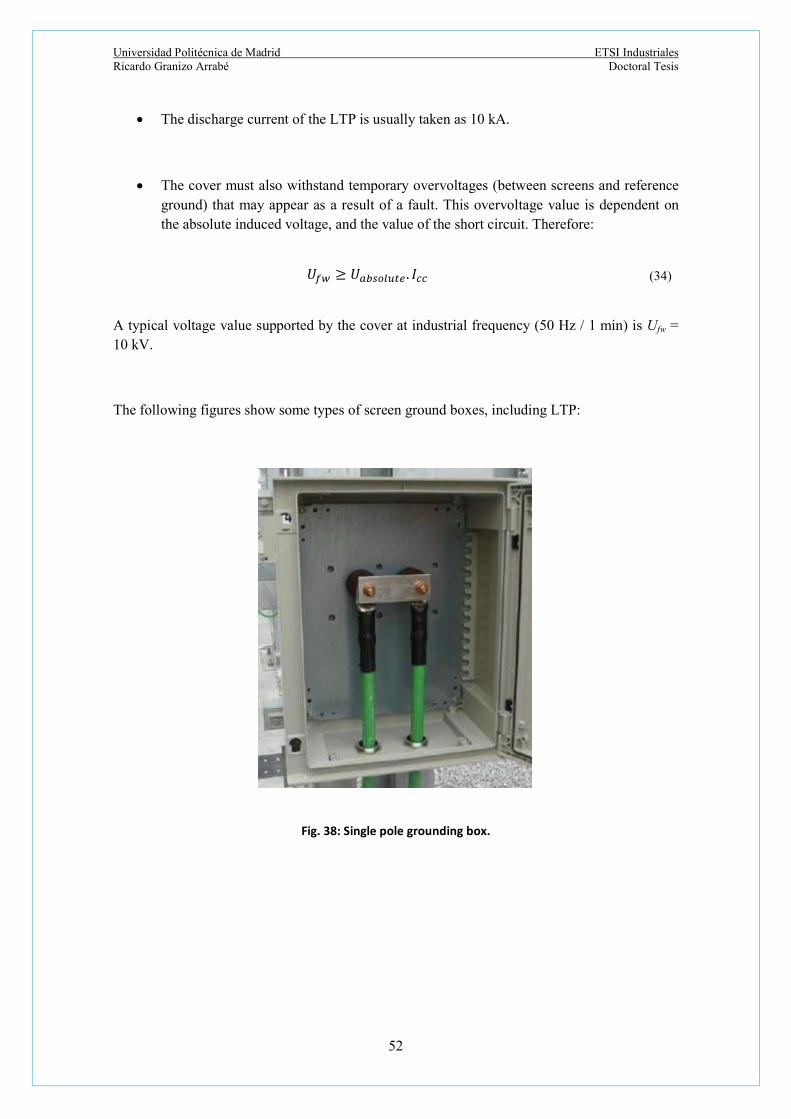
Universidad Politécnica de Madrid ETSI Industriales Ricardo Granizo Arrabé Doctoral Tesis
52
The discharge current of the LTP is usually taken as 10 kA.
The cover must also withstand temporary overvoltages (between screens and reference ground) that may appear as a result of a fault. This overvoltage value is dependent on the absolute induced voltage, and the value of the short circuit. Therefore:
𝑈 ≥ 𝑈 . 𝐼 (34)
A typical voltage value supported by the cover at industrial frequency (50 Hz / 1 min) is Ufw = 10 kV.
The following figures show some types of screen ground boxes, including LTP:
Fig. 38: Single pole grounding box.

Universidad Politécnica de Madrid ETSI Industriales Ricardo Granizo Arrabé Doctoral Tesis
53
Fig. 39: Three pole grounding box.
Fig. 40: Single pole grounding box with LTP.
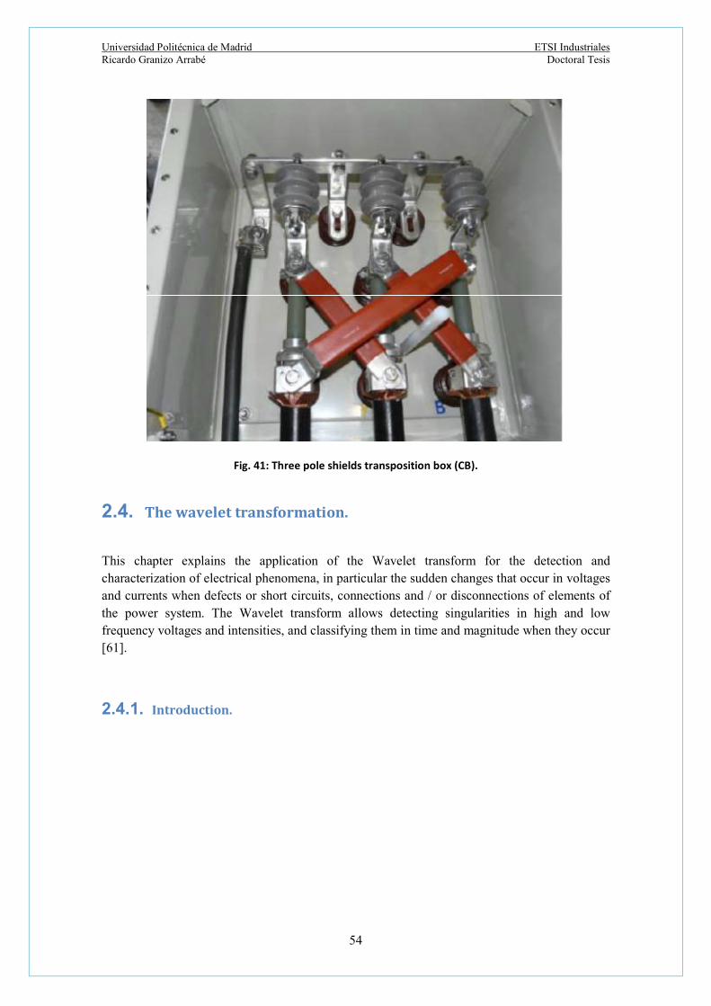
Universidad Politécnica de Madrid ETSI Industriales Ricardo Granizo Arrabé Doctoral Tesis
54
Fig. 41: Three pole shields transposition box (CB).
2.4. The wavelet transformation.
This chapter explains the application of the Wavelet transform for the detection and characterization of electrical phenomena, in particular the sudden changes that occur in voltages and currents when defects or short circuits, connections and / or disconnections of elements of the power system. The Wavelet transform allows detecting singularities in high and low frequency voltages and intensities, and classifying them in time and magnitude when they occur [61].
2.4.1. Introduction.

Universidad Politécnica de Madrid ETSI Industriales Ricardo Granizo Arrabé Doctoral Tesis
55
Traditionally, different methods of analysis of power electrical systems have been used, using algorithms based on different transformations of the data corresponding to the evaluated signals. The most used mathematical transformation has been and still is today, the Fourier transform in any of its multiple variants. In the transient analysis of electrical phenomena, the signals that are presented usually do not have the slightest perioricity. Such transient signals may have high oscillation content over a very wide and disparate frequency range. These frequency oscillations are perfectly characterized by the Fourier transform from the point of view of the evaluation of the harmonic content in frequency. Unfortunately, the Fourier transform does not allow locating in time the said evaluation of the harmonic content during the transient phenomena.
In contrast, the signal analysis using the Wavelet Transform does allow it since it is able to provide information of both the frequency content and the times in which these contents of the evaluated signal appear and disappear [62]. Thanks to this potential, the Wavelet Transform allows analyzing and interpreting a large variety of transient phenomena that can occur in power electrical systems and, in particular, in electrical transmission and distribution networks [63], [64].
2.4.2. Representation of signals in the time domain.
It is the simplest representation of the phenomena that are studied and analyzed. It suffices to be able to represent in Cartesian axes the relation that keeps the amplitude of the studied variable and the time in which that amplitude is presented. Analytically speaking, we work in the time-amplitude domain as shown in the following figure.
Fig. 42: Temporal representation. Time-Domain.
0 0.05 0.1 0.15 0.2 0.25 0.3 0.35 0.4 0.45 0.5-150
-100
-50
0
50
100
150
Time (s)
y(t)
y=100·sin(2·pi·50·t)+20·cos(2·pi·150·t)

Universidad Politécnica de Madrid ETSI Industriales Ricardo Granizo Arrabé Doctoral Tesis
56
2.4.3. Fourier and his transformation.
Literally speaking, the Fourier Transform [65] allows the decomposition of any signal, in sums of sinusoidal characteristic signals each of different frequency. Its general mathematical expression is:
𝐹(𝜔) = ∫ 𝑓(𝑡) · 𝑒 𝑑𝑡 (2)
Logically, from the already decomposed signal, the original signal can be reconstructed if the following expression is applied:
𝐹(𝑡) = ∫ 𝑓(𝜔) · 𝑒 𝑑𝜔 (3)
The following graphs show different representations of signals in the fields or domains temporal and frequency:
Fig. 43: Signal analyzed: 𝒚(𝒕) = 𝟎. 𝟕 · 𝒔𝒊𝒏(𝟏𝟎𝟎 · 𝝅 · 𝒕) + 𝒔𝒊𝒏(𝟐𝟒𝟎 · 𝝅 · 𝒕).
0 0.1 0.2 0.3 0.4 0.5 0.6 0.7 0.8 0.9 1-2
-1.5
-1
-0.5
0
0.5
1
1.5
2
Time (s)
y(t)
Signal y(t)=0.7*sin(100·pi·t)+sin(240·pi·t)
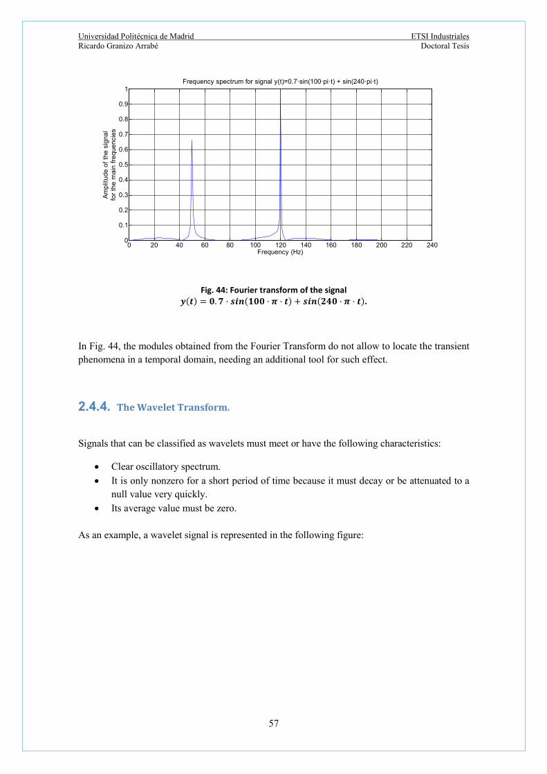
Universidad Politécnica de Madrid ETSI Industriales Ricardo Granizo Arrabé Doctoral Tesis
57
Fig. 44: Fourier transform of the signal
𝒚(𝒕) = 𝟎. 𝟕 · 𝒔𝒊𝒏(𝟏𝟎𝟎 · 𝝅 · 𝒕) + 𝒔𝒊𝒏(𝟐𝟒𝟎 · 𝝅 · 𝒕).
In Fig. 44, the modules obtained from the Fourier Transform do not allow to locate the transient phenomena in a temporal domain, needing an additional tool for such effect.
2.4.4. The Wavelet Transform.
Signals that can be classified as wavelets must meet or have the following characteristics:
Clear oscillatory spectrum.
It is only nonzero for a short period of time because it must decay or be attenuated to a null value very quickly.
Its average value must be zero.
As an example, a wavelet signal is represented in the following figure:
0 20 40 60 80 100 120 140 160 180 200 220 2400
0.1
0.2
0.3
0.4
0.5
0.6
0.7
0.8
0.9
1Frequency spectrum for signal y(t)=0.7·sin(100·pi·t) + sin(240·pi·t)
Frequency (Hz)
Am
plit
ude
of
the
sign
al
for
the
mai
n f
req
uenc
ies

Universidad Politécnica de Madrid ETSI Industriales Ricardo Granizo Arrabé Doctoral Tesis
58
Fig. 45: Signal analysis using Wavelet Daubechies dB4.
As shown in the previous figure, wavelet functions are used to develop time-scale domain analysis [66].
2.4.5. Fundamentals of the Wavelet Transform.
Signal analysis employing the Wavelet Transform represents signals as a function of other reference or pattern signals, which:
They move in time.
They are scaled in different amplitudes.
The objective is to compare a wave with another type pattern, originated by iterating the different dilations obtained from a specific function of staggering along the axis of abscissa. The iterations are terminated when. It should be noted that the final shape of the pattern depends on the number of scales or scaling coefficients that have been used to generate said staggering function. The more coefficients or scales are selected, the signal will be smoother. In contrast, when fewer the coefficients are used the signal will be much steeper. Let's see two wavelets of the family "Coiflet" [67].
0.4995 0.4996 0.4997 0.4998 0.4999 0.5 0.5001 0.5002 0.5003 0.5004 0.5005-2
-1.5
-1
-0.5
0
0.5
1
1.5
Time (s)
Coe
ffic
ien
ts c
D1
wav
ele
t D
au
be
chie
s d
B4
Signal analysis using wavelet Daubechies dB4
cD1-dB4 coefficients

Universidad Politécnica de Madrid ETSI Industriales Ricardo Granizo Arrabé Doctoral Tesis
59
Fig. 46: Signal analysis using Wavelet Coiflet1.
Fig. 47: Signal analysis using Wavelet Coiflet5.
Between Fig. 46 and Fig. 47 are similarities but better defined response is observed and without so many intermediate oscillations when using a lower level wavelet (Coiflet 1 in this case). For transient analyses, normally the Wavelet that detects them best is the Daubechies. Logically, the choice of a Wavelet or another depends on the type of signals that are analyzed. Once the Wavelet that best answers our analysis is selected, the process of moving and scaling is started to compare it with the original signal of analysis. If this operation is performed successively, we obtain the coefficients of the Discrete Wavelet Transformation (DWT) whose mathematical definition is:
0.4995 0.4996 0.4997 0.4998 0.4999 0.5 0.5001 0.5002 0.5003 0.5004 0.5005-2
-1.5
-1
-0.5
0
0.5
1
1.5
Time (s)
Coe
ffic
ien
ts W
ave
let
Coi
flet
1 s
cale
32
Signal analysis using wavelet Coiflet 1
Coiflet1 - scale 32
0.4995 0.4996 0.4997 0.4998 0.4999 0.5 0.5001 0.5002 0.5003 0.5004 0.5005-1.5
-1
-0.5
0
0.5
1
1.5
Time (s)
Coe
ffic
ien
ts W
ave
let
Coi
flet
5 s
cale
32
Signal analysis using Wavelet Coiflet 5
Coiflet 5 - Scale 32

Universidad Politécnica de Madrid ETSI Industriales Ricardo Granizo Arrabé Doctoral Tesis
60
dta
bttf
abaW
1
, (37)
With:
a: coefficient of expansion.
b: delay in the Signal.
1 / √a: normalization coefficient.
With these coefficients already known, the original signal is decomposed into different levels associated with different frequency ranges. The higher decomposition levels correspond to the higher frequency levels. The number of decay stages is chosen according to the sampling frequency of the original signal. The first decomposition has two elements, a high frequency element D1 and a low frequency element A1. Depending on the sampling frequency fs, the frequency band of the element D1 is fs / 2 - fs / 4 Hz, while the frequency band of the element A1 is fs / 4 - 0 Hz. In the second decomposition, the element A1 is decomposed into high frequency band elements D2 (fs / 4 - fs / 8 Hz) and the element A2 for the low frequency band (fs / 8 - 0 Hz). This process is repeated until the desired frequency band allows the correct information to be extracted from the evaluated signal.
2.4.6. Main application of the Wavelet Transform.
Its main application in electrical systems lies in the detection of a large number of perturbations in which the effective and instantaneous values of the forms evaluated increase or decrease considerably [68]. Typically, such disturbances are:
- Voltage drops.
- Short power interruptions.
- Lightnings strokes.
- Switching on and off different power elements in the grids.
- Short-circuits.
Such detections can be achieved because the Wavelet Transform:
- It is able to represent functions.
- It may represent irregularities or signal singularities.

Universidad Politécnica de Madrid ETSI Industriales Ricardo Granizo Arrabé Doctoral Tesis
61
- It allows detecting changes and discontinuities in second derivatives.
- It allows detecting changes of frequencies.
- It is able to detect superimposed signals of short duration.
- It allows compressing data.
- It manages not to lose information in time.
Thanks to these characteristics, the application of the Wavelet Transform in the analysis of the electrical systems is already a common practice.
2.4.7. Example of analysis using the Wavelet Transform.
In the circuit of Fig. 48 the connection of a capacity to two resistive loads connected in parallel.
Fig. 48: Sample electrical circuit for analysis of swicthing-on a capacitor.
Fig. 49 shows the evolution of the voltage at node A once the capacity is connected at time t = 500 ms.
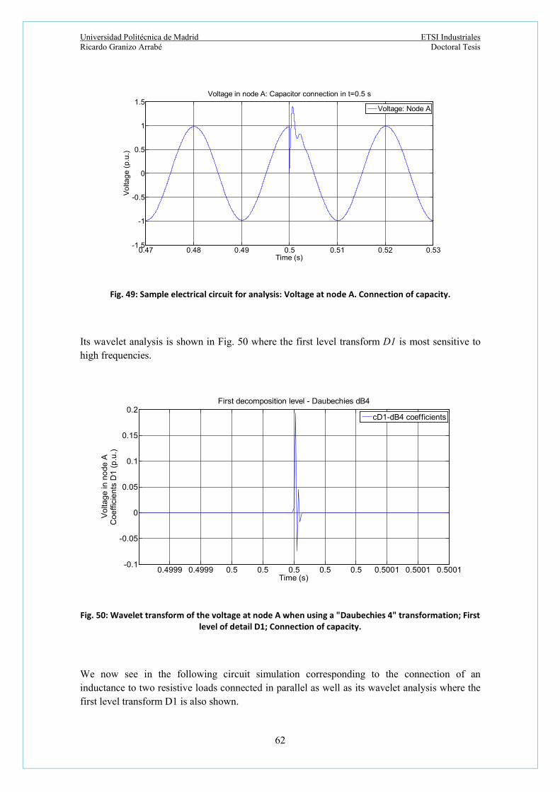
Universidad Politécnica de Madrid ETSI Industriales Ricardo Granizo Arrabé Doctoral Tesis
62
Fig. 49: Sample electrical circuit for analysis: Voltage at node A. Connection of capacity.
Its wavelet analysis is shown in Fig. 50 where the first level transform D1 is most sensitive to high frequencies.
Fig. 50: Wavelet transform of the voltage at node A when using a "Daubechies 4" transformation; First
level of detail D1; Connection of capacity.
We now see in the following circuit simulation corresponding to the connection of an inductance to two resistive loads connected in parallel as well as its wavelet analysis where the first level transform D1 is also shown.
0.47 0.48 0.49 0.5 0.51 0.52 0.53-1.5
-1
-0.5
0
0.5
1
1.5
Time (s)
Vo
ltag
e (
p.u
.)
Voltage in node A: Capacitor connection in t=0.5 s
Voltage: Node A
0.4999 0.4999 0.5 0.5 0.5 0.5 0.5 0.5001 0.5001 0.5001-0.1
-0.05
0
0.05
0.1
0.15
0.2
Time (s)
Vo
ltag
e in
no
de
AC
oe
ffic
ien
ts D
1 (
p.u
.)
First decomposition level - Daubechies dB4
cD1-dB4 coefficients

Universidad Politécnica de Madrid ETSI Industriales Ricardo Granizo Arrabé Doctoral Tesis
63
Fig. 51: Sample electrical circuit for analysis: Connection of inductance.
The voltage at node A and its wavelet analysis are shown in Fig. 52 and 53.
Fig. 52: Sample electrical circuit for analysis; Voltage at node A; Connection inductance.
0.4 0.42 0.44 0.46 0.48 0.5 0.52 0.54 0.56 0.58 0.6-1
-0.5
0
0.5
1
Time (s)
Vo
ltage
in p
.u.
in n
od
e A
Voltage in node A: Connection of an inductance in t=0.5 s.
Voltage Node A
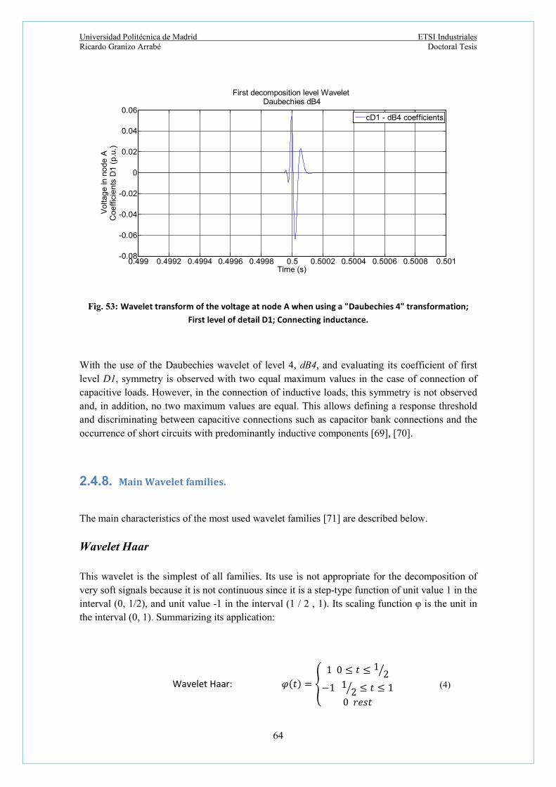
Universidad Politécnica de Madrid ETSI Industriales Ricardo Granizo Arrabé Doctoral Tesis
64
Fig. 53: Wavelet transform of the voltage at node A when using a "Daubechies 4" transformation;
First level of detail D1; Connecting inductance.
With the use of the Daubechies wavelet of level 4, dB4, and evaluating its coefficient of first level D1, symmetry is observed with two equal maximum values in the case of connection of capacitive loads. However, in the connection of inductive loads, this symmetry is not observed and, in addition, no two maximum values are equal. This allows defining a response threshold and discriminating between capacitive connections such as capacitor bank connections and the occurrence of short circuits with predominantly inductive components [69], [70].
2.4.8. Main Wavelet families.
The main characteristics of the most used wavelet families [71] are described below.
Wavelet Haar
This wavelet is the simplest of all families. Its use is not appropriate for the decomposition of very soft signals because it is not continuous since it is a step-type function of unit value 1 in the interval (0, 1/2), and unit value -1 in the interval (1 / 2 , 1). Its scaling function φ is the unit in the interval (0, 1). Summarizing its application:
Wavelet Haar: 𝜑(𝑡) =
1 0 ≤ 𝑡 ≤ 12
−1 12 ≤ 𝑡 ≤ 1
0 𝑟𝑒𝑠𝑡
(4)
0.499 0.4992 0.4994 0.4996 0.4998 0.5 0.5002 0.5004 0.5006 0.5008 0.501-0.08
-0.06
-0.04
-0.02
0
0.02
0.04
0.06
Time (s)
Vo
ltag
e in
no
de
AC
oe
ffici
en
ts D
1 (
p.u
.)
First decomposition level Wavelet Daubechies dB4
cD1 - dB4 coefficients

Universidad Politécnica de Madrid ETSI Industriales Ricardo Granizo Arrabé Doctoral Tesis
65
Fig. 54: Wavelet Haar.
Wavelet Daubechies
The Daubechies wavelet of order M presents a number of null moments of value M and its application is interesting and appropriate for soft signals.
Fig. 55: Wavelet Daubechies.
Wavelet Coiflets
The Coiflet wavelet is very similar to the Daubechies presenting mere differences as it can be the fact of presenting greater symmetry and having less number of null moments.

Universidad Politécnica de Madrid ETSI Industriales Ricardo Granizo Arrabé Doctoral Tesis
66
Fig. 56: Wavelet Coiflet
2.4.9. Detection ofdisturbances.
One of the main characteristics of the Wavelet Transform is its application in the detection of transient phenomena and disturbances in electrical networks such as voltage gaps, short duration interruptions, surges, short circuits, etc [72]. In order to detect these events, it is first necessary to know:
The wavelet transform is to be used. The main characteristics of the signals to be analyzed
The objectives that are pursued. Of vital importance is to establish a threshold that allows considering that an event has been detected if it has been exceeded, and, if not exceeded, the different values of the signal or analyzed signals will not be considered. The first level of detail in the decomposition of a signal allows detection and localization in sufficient time [73]. Fig. 57 corroborates this detection and location by applying a single level of detail to an actual voltage signal corresponding to a single-phase ground fault in a 220 kV network. In this figure the detections of the beginning and ending of the fault are clearly observed.
Fig. 57: Single-phase ground fault detection in a 220 kV grid using a Daubechies db6 wavelet.
2.4.10. Signal detection of events and changes.

Universidad Politécnica de Madrid ETSI Industriales Ricardo Granizo Arrabé Doctoral Tesis
67
For the optimal choice of Wavelet Transform to be used, it is firstly necessary to know what type of signals to analyze and what results are intended to be achieved. Secondly it is imperative to select a threshold such that with values greater than the same it is considered that the event has been detected and with values lower than said threshold it is considered that no event has been detected.
The first level of decomposition relative to detection and location is adequate to detect a disturbance and localize it over time. This is so since the first-level decomposition coefficients correspond to the highest frequency disturbances [74].
Finally, it is necessary to identify the frequency bands for a given wavelet decomposition in order to be able to adjust the detection band to the event or signal change that is to be identified.
2.4.11. Selection of the Wavelet function.
To make the best possible selection of the mother wavelet to be used in the detection of events or signal changes, it is necessary to evaluate the values of the coefficients of the signal decomposition at different levels [75]. Thus, if a signal presents a discrete wavelet transform (DWT) that is null for practically all coefficients and not null for a small number of them, the signal is very centered and localized in the time-frequency space. This provides increased signal-to-noise gain at detection peaks by increasing the chance of detecting such events. In contrast, a discrete wavelet transform with many nonzero coefficients means that the signal is much dispersed, and perhaps the noise can be confused with the events to be captured.
The wavelets normally used in the detection and locations of events in electrical systems are:
- Daubechies 2, 4 and 6: employed in detection and localization.
- Daubechies 8 and 10: employed in slow transient analyses.
Since there are many options for selecting wavelets, the best possible option is the one that most closely approximates the waveform to be analyzed. For this, the process that follows is as follows:
a) Calculation of the wavelet coefficients.
b) Selection of the threshold that determines the detection of the event.
c) Elimination of the values of those coefficients lower than the selected threshold.Choice of the wavelet with the highest number of null coefficients.
When evaluating real signals, noise is always more or less measured. Thus, in order to have a good visualization and detection of desired electrical phenomena or events, it is common practice to use squared wavelet coefficients [76].

Universidad Politécnica de Madrid ETSI Industriales Ricardo Granizo Arrabé Doctoral Tesis
68
The reason for its use lies in that the peaks are made much easier to distinguish compared to the background coefficients. In this way, it can be affirmed that the wavelet coefficients with low values are due to the electrical noise of the signal analyzed while the high value wavelet coefficients are synonymous with the presence of electrical disturbances.
When the wavelet coefficients represent the variations with respect to the mean, the largest coefficient of all of them is due to a significant change in the signal analyzed. The moments at which such abrupt changes in the signal occur can be assigned to the coefficients that exceed a predetermined and predetermined threshold U. If the coefficients do not exceed this threshold U, these can be assimilated to zero and thus the details that are considered as noise are not considered.
It is an important task to determine the most interesting threshold for the detection of the event under study [77], [78]. Its determination is made first by defining a filtering criterion and then defining the threshold function U to be used.
There are two filtering criteria: the hard criterion and the soft criterion. The hard criterion is based on the direct comparison of the coefficients with the threshold and the soft criterion reduces the value of all the coefficients in order to eliminate the noise. Their formulations are:
Hard filtering: 𝑥 =𝑥 𝑠𝑖 |𝑥| > 𝑈0 𝑠𝑖 |𝑥| ≤ 𝑈
(38)
Soft filtering: 𝑥 =𝑥 − 𝑈 𝑠𝑖 𝑥 > 𝑈
𝑥 + 𝑈 𝑠𝑖 𝑥 < −𝑈0 𝑠𝑖 |𝑥| ≤ 𝑈
(39)
The value of the threshold U is selected such that its value encounters a high probability immediately above the maximum noise value of the coefficients. The universal threshold UU selected [79] depends on the mean of the absolute deviation and the number N of samples of the wavelet coefficients. It has the next formulation:
Threshold: 𝑈 = 𝜎 2𝑙𝑜𝑔𝑁 (40)
2.4.12. Example of mother wavelet selection.
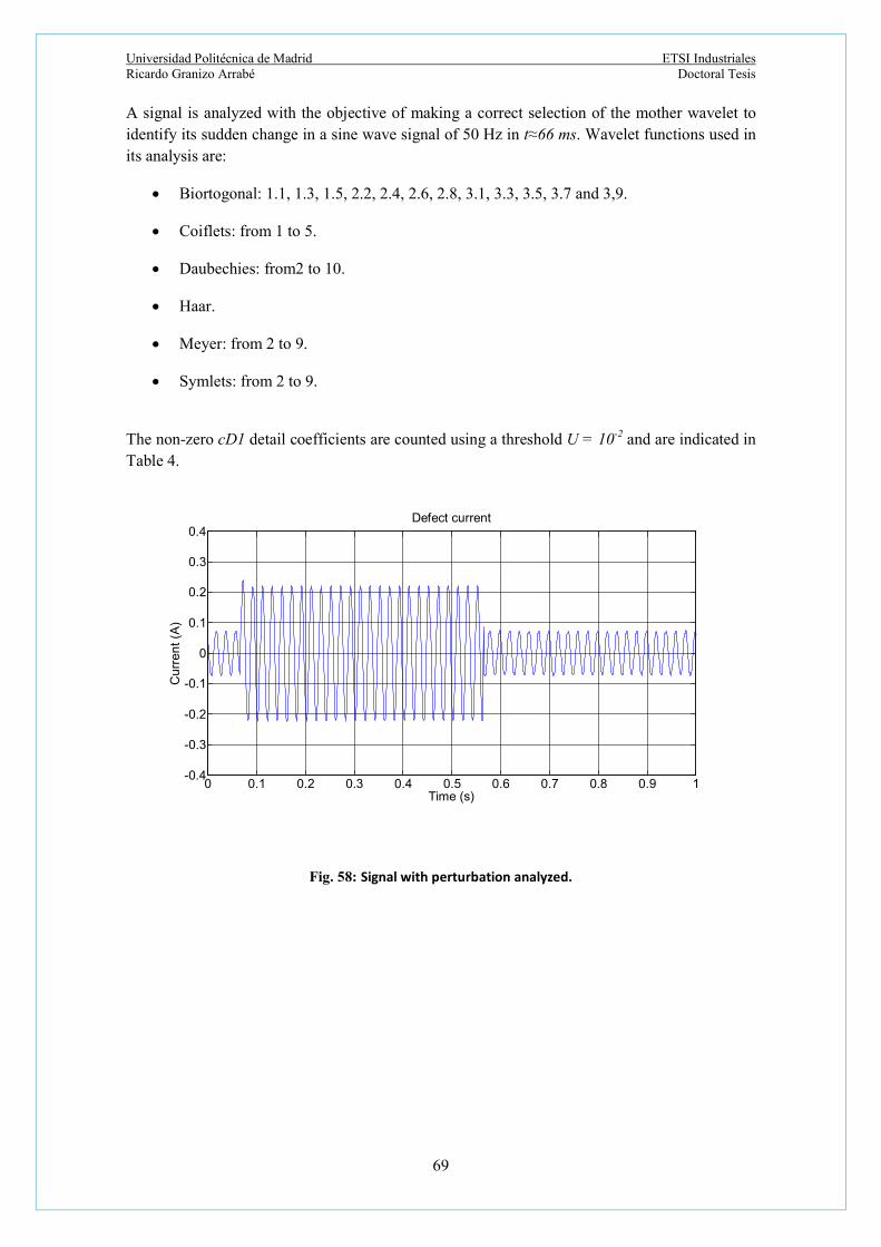
Universidad Politécnica de Madrid ETSI Industriales Ricardo Granizo Arrabé Doctoral Tesis
69
A signal is analyzed with the objective of making a correct selection of the mother wavelet to identify its sudden change in a sine wave signal of 50 Hz in t≈66 ms. Wavelet functions used in its analysis are:
Biortogonal: 1.1, 1.3, 1.5, 2.2, 2.4, 2.6, 2.8, 3.1, 3.3, 3.5, 3.7 and 3,9.
Coiflets: from 1 to 5.
Daubechies: from2 to 10.
Haar.
Meyer: from 2 to 9.
Symlets: from 2 to 9.
The non-zero cD1 detail coefficients are counted using a threshold U = 10-2 and are indicated in Table 4.
Fig. 58: Signal with perturbation analyzed.
0 0.1 0.2 0.3 0.4 0.5 0.6 0.7 0.8 0.9 1-0.4
-0.3
-0.2
-0.1
0
0.1
0.2
0.3
0.4
Time (s)
Cu
rre
nt
(A)
Defect current

Universidad Politécnica de Madrid ETSI Industriales Ricardo Granizo Arrabé Doctoral Tesis
70
Table 4: Non-zero detail coefficients cD1 at the first filtering level.
Wavelet cD1 not null
Wavelet cD1 not null
Wavelet cD1 not null
bior1.1 461 coif1 5 db9 7
bior1.3 461 coif2 3 db10 7
bior1.5 461 coif3 6 Haar 461
bior2.2 3 coif4 6 dmey 9
bior2.4 3 coif5 6 sym2 5
bior2.6 3 db2 5 sym3 3
bior2.8 3 db3 3 sym4 4
bior3.1 4 db4 6 sym5 6
bior3.3 4 db5 6 sym6 5
bior3.5 4 db6 7 sym7 7
bior3.7 4 db7 7 sym8 5
bior3.9 4 db8 7 sym9 6
According to the results shown in Table 4, the use of the bior1.1, bior1.3, bior1.5, db6, db7, db8, db9, db10, Haar, dmey (Meyer) and sym7 wavelets is not recommended to detect disturbance of the analyzed signal. The remaining wavelets are applicable for the detection of the exposed disturbance.
In Fig. 59 and 60 the total coefficients db3-cD1 and a zoom of the three non-zero coefficients detected by the Daubechies db3 wavelet are shown.
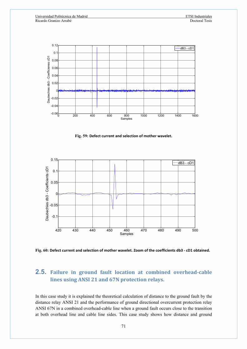
Universidad Politécnica de Madrid ETSI Industriales Ricardo Granizo Arrabé Doctoral Tesis
71
Fig. 59: Defect current and selection of mother wavelet.
Fig. 60: Defect current and selection of mother wavelet. Zoom of the coefficients db3 - cD1 obtained.
2.5. Failure in ground fault location at combined overhead-cable lines using ANSI 21 and 67N protection relays.
In this case study it is explained the theoretical calculation of distance to the ground fault by the distance relay ANSI 21 and the performance of ground directional overcurrent protection relay ANSI 67N in a combined overhead-cable line when a ground fault occurs close to the transition at both overhead line and cable line sides. This case study shows how distance and ground
0 200 400 600 800 1000 1200 1400 1600-0.06
-0.04
-0.02
0
0.02
0.04
0.06
0.08
0.1
0.12
Samples
Dau
bech
ies
db3
- C
oeff
icie
nes
cD1
dB3 - cD1
420 430 440 450 460 470 480 490 500
-0.1
-0.05
0
0.05
0.1
0.15
Samples
Dau
be
chie
s d
b3
- C
oe
ffici
en
ts c
D1
dB3 - cD1

Universidad Politécnica de Madrid ETSI Industriales Ricardo Granizo Arrabé Doctoral Tesis
72
directional overcurrent protection relays are not suitable to grant correct auto-reclosing orders to the main circuit breaker as they are able to detect and clear the ground fault but without accuracy enough to know in which side of the line took place the ground fault.
2.5.1. Theoretical study.
For this case study it has selected a typical power distribution network rated 20 kV with the next basic features:
Table 5: 20 kV power distribution network: basic parameters.
Parameters:
Un=20 kV Scc=500 MVA X/R=10 f=50 Hz Grounding connection: YN
The values obtained for the resistance and reactance of the grid are:
Grid Resistance: 0.0876 Ω
Grid Reactance: 0.8756 Ω
The conductor data of the overhead line side considered for this theoretical study is a conductor type LA56. Its main data are listed in Table 6:
Table 6: Conductor LA56. Main features.
Conductor Total Section (mm2)
Resistance at 20ºC (Ω/km)
Resistance at 50ºC (Ω/km)
Outer diameter
(mm)
Max. Current (A)
LA-56 54,6 0,613 0,687 9,45 199,35
Next figure shows the dimensions of the tower selected for this case study:

Universidad Politécnica de Madrid ETSI Industriales Ricardo Granizo Arrabé Doctoral Tesis
73
Fig. 61: Power distribution Network rated 20 kV: Dimensions of tower used.
This distribution overhead line side and electrical tower disposals have the next values:
Table 7: Overhead-line features.
Length: 20 km Span: 100 m Max. arrow in conductors: 1,97 m Soil resistivity: 100 Ω.m
Using the tool Power Line Parameters from Matlab, the values obtained for the RLC parameters of this overhead line are:
Table 8: Overhead-line RLC features.
Positive resistance sequence (Ω/km): 0.68712 Zero resistance sequence (Ω/km): 0.83102 Positive inductance sequence (H/km): 0.0013089 Zero inductance sequence (H/km): 0.0048614 Positive capacitance sequence (F/km): 8.8981e-009 Zero capacitance sequence (F/km): 4.2434e-009
For the total length of 20 km, the impedance of the overhead line has the next value:

Universidad Politécnica de Madrid ETSI Industriales Ricardo Granizo Arrabé Doctoral Tesis
74
𝑍 , = 13.7424 + 8.2241𝑗 Ω
(5)
The network used in this case study is represented in Fig. 62:
Fig. 62: Ground fault at the end of the overhead line side.
For a phase-to-ground fault at the end of the overhead line side in phase “a” as example, the symmetrical components obtained are:
The symmetric components of the voltages at the place where the protection relay ANSI 21 and ANSI 67 is installed are:
The protection relay also evaluates the current in phase a:
I1=I2=I0=174.21∟-45.15º
(42)
𝐸𝐸𝐸
=
11439 . º
153.30 . º
153.30 . º
𝑉
(43)
𝐼 𝐼 · 3 = 522.62 . º A
(44)

Universidad Politécnica de Madrid ETSI Industriales Ricardo Granizo Arrabé Doctoral Tesis
75
With:
The compensation factor m for the zero sequence compensation in:
Therefore the compensated current in phase “a” is:
Finally, the impedance seen by the distance protection relay ANSI 21 has the next value:
This value corresponds exactly to the total length of the overhead line. However, the protection relay ANSI 21 receives the voltages and currents of the overhead line from voltage transformers and current transformers. For this example we suppose a load of 1.26 MVA that corresponds to 36.4 A. The transformation ratios of voltage and current transformers are set to:
Voltage transformer (VT): 22000 √3⁄ − 110 √3⁄ 𝑉
Current transformer (CT): 50 5⁄ 𝐴
With such ratios, the protection relay ANSI 21 receives the next signals:
𝐼 = √
, · , , · ,=174.21 . º A (45)
𝑚 =𝑍 − 𝑍
𝑍= 1.4053 . º (46)
𝐼 = 𝐼 + 𝑚 · 𝐼 = 701.04 . º 𝐴
(47)
𝑍 =𝐸
𝐼=
𝐸 + 𝐸 + 𝐸
𝐼= 13.7424 + 8.2241𝑗 = 16.0153 . º Ω
(48)
𝐸 , = 11227 . º ·110
22000= 56.137 . º𝑉
(49)

Universidad Politécnica de Madrid ETSI Industriales Ricardo Granizo Arrabé Doctoral Tesis
76
The correction of the current in phase “a” is done accordingly:
The impedance seen at the relay side is:
This value transferred to primary side corresponds to:
So far, all data calculated shows clear correspondence but the error in the measuring of voltages and currents from the VT´s and CT´s can´t be neglected for this application. If we consider that the VT has +1% error and the CT -1% error in the transforming ratios but keeping almost zero the phase error, the magnitudes that the protection relay ANSI 21 receives are:
Now, the correction of the current in phase “a” is done accordingly considering the error of the CT:
The impedance seen at the relay side considering those errors is:
𝐼 , = 522.62 . º ·5
50= 52.262 . º𝐴
(50)
𝐼 , = 𝐼 , + 𝑚 · 𝐼 , = 70.1043 . º 𝐴
(51)
𝑍 =𝐸 ,
𝐼 ,
= 0.8008 . º Ω
(52)
𝑍 , = 𝑍 ·22000
110·
5
50= 16.0153 . º Ω
(53)
𝐸 %, = 1.01 · 11227 . º ·110
22000= 56.698 . º𝑉
(54)
𝐼 %, = 0.99 · 522.62 . º ·5
50= 51.739 . º𝐴
(55)
𝐼 %, = 𝐼 %, + 𝑚 · 𝐼 %, = 69.4032 . º 𝐴
(56)

Universidad Politécnica de Madrid ETSI Industriales Ricardo Granizo Arrabé Doctoral Tesis
77
This value transferred to primary side now corresponds to:
The difference in the calculation of the impedance is:
This value transferred to primary side now corresponds to:
The difference in the calculation of the impedance is:
This difference in the impedance calculated represents the outstanding distance of 402.74 m. We must highlight that only considering a minimum error in the VT´s and CT´s can cause an error in the distance from the protection relay to the ground fault over 400 m in the range of 2%, it can be 400 m increase or 400 m decrease. This represents a range in the impedance measured that can drive to the protection relay ANSI 21 to develop an auto-reclosing manoeuvre with the uncertainty of knowing at which side of the line has occurred the ground fault. Therefore, this high risk can´t be taken up by the protection relay. So this protection relay is able to detect and clear up the ground fault but can´t discriminate properly where it happened.
Regarding the functionality of the ground directional overcurrent protection (ANSI 67N), the symmetric components obtained before for the residual current and voltage at the place where the protection relay ANSI 67N is installed are:
𝑍 , =𝐸 %,
𝐼 %,
= 0.8169 . º Ω
(57)
𝑍 , , = 𝑍 , ·22000
110·
5
50= 16.3388 . º Ω
(58)
𝑍 , =𝐸 %,
𝐼 %,
= 0.8169 . º Ω
(59)
𝑍 , , = 𝑍 , ·22000
110·
5
50= 16.3388 . º Ω
(60)
𝑍 , − 𝑍 , , = 0.3225 Ω
(61)

Universidad Politécnica de Madrid ETSI Industriales Ricardo Granizo Arrabé Doctoral Tesis
78
𝐸 = 153.30 . ºV
𝐼 = 174 . ºA
For a power distribution network solidly grounded, the Relay Characteristic Angle (RCA) is normally 110º lagging the defect current I0 respect the residual voltage E0. This RCA is shown in Fig. 63.
Fig. 63: Relay Characteristic Angle (RCA) in solidly grounded power distribution networks.
Considering the errors granted by the current and voltage transformers manufacturers indicated in Tables 9 and 10, it can be considered the next errors in phase:
Table 9: Current transformer. Phase displacement in minutes by EN61869-2.
Class Error in ratio (%)
1.00 x In
Phase displacement
(Minutes)
1.00 x In
Compound error (%) and limit for nominal precision
P x In
5P 1.0 60 5
10P 3.0 - 10
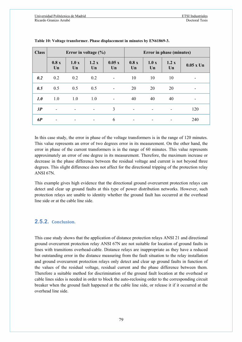
Universidad Politécnica de Madrid ETSI Industriales Ricardo Granizo Arrabé Doctoral Tesis
79
Table 10: Voltage transformer. Phase displacement in minutes by EN61869-3.
Class Error in voltage (%) Error in phase (minutes)
0.8 x Un
1.0 x Un
1.2 x Un
0.05 x Un
0.8 x Un
1.0 x Un
1.2 x Un
0.05 x Un
0.2 0.2 0.2 0.2 - 10 10 10 -
0.5 0.5 0.5 0.5 - 20 20 20 -
1.0 1.0 1.0 1.0 - 40 40 40 -
3P - - - 3 - - - 120
6P - - - 6 - - - 240
In this case study, the error in phase of the voltage transformers is in the range of 120 minutes. This value represents an error of two degrees error in its measurement. On the other hand, the error in phase of the current transformers is in the range of 60 minutes. This value represents approximately an error of one degree in its measurement. Therefore, the maximum increase or decrease in the phase difference between the residual voltage and current is not beyond three degrees. This slight difference does not affect for the directional tripping of the protection relay ANSI 67N.
This example gives high evidence that the directional ground overcurrent protection relays can detect and clear up ground faults at this type of power distribution networks. However, such protection relays are unable to identity whether the ground fault has occurred at the overhead line side or at the cable line side.
2.5.2. Conclusion.
This case study shows that the application of distance protection relays ANSI 21 and directional ground overcurrent protection relay ANSI 67N are not suitable for location of ground faults in lines with transitions overhead-cable. Distance relays are inappropriate as they have a reduced but outstanding error in the distance measuring from the fault situation to the relay installation and ground overcurrent protection relays only detect and clear up ground faults in function of the values of the residual voltage, residual current and the phase difference between them. Therefore a suitable method for discrimination of the ground fault location at the overhead or cable lines sides is needed in order to block the auto-reclosing order to the corresponding circuit breaker when the ground fault happened at the cable line side, or release it if it occurred at the overhead line side.

Universidad Politécnica de Madrid ETSI Industriales Ricardo Granizo Arrabé Doctoral Tesis
80
2.6. Switch on to fault schemes in protection functions.
Switch-on-to-fault (SOTF) schemes are protection functions that are thought to release a tripping command to circuitbreakers when the closing of such circuitbrekers are developed on faulted conditions. Normally SOTF schemes are only active short time after the closing of the corresponding circuitbreaker. Their main application corresponds to transmission and distribution lines [80].
2.6.1. Applications of SOFT protection schemes.
There are three main reasons to implement SOFT protection schemes are:
1. When distance protection relays receive line voltages from voltage transformers installed at the line side the use of SOFT protection schemes is needed to detect and clear very close three-phase faults when the circuibreaker is closed into such heavy fault. Under this type of severe fault, there is total absence of voltage read by the distance protection relay and therefore it will not neither see the fault nor send a tripping command to the circuitbreaker. The result turns out to be a time-delayed tripping command at different remote substations with the consequent instability and possible collapse in the grid as well as the loss of power supply in several areas.
2. SOFT overcurrent detection scheme operates quicker than distance protection relays. This fact is due to the low speed of operation of distance protection relays when the polarization voltages are not available before the fault takes place. If the grid is weak and its equivalent source impedance is high, the overcurrent setting must be low.
3. In any line protection application, independent of the voltage transformers emplacement, SOFT protection schemes allow detecting and clearing faults along the complete length of the line without delays owing to communications tripping schemes. Normal settings for overcurrent or distance protection relays must cover the entire line [81].
Sometimes there are difficult operation conditions of the grid when there is a combination of reduced voltage at the busbars of the substation and the necessity of coupling some lines to such busbars. SOFT protection schemes must not operate in a wrong way when the circuit breaker receives the closing command from the control center or from an automatic reclosing relay. It can be achieved if:
- SOFT protection scheme is only used after closing the circuitbreaker.
- SOFT line voltage detection must be set lower than the maximum voltage level expected when lines are open at the other end.

Universidad Politécnica de Madrid ETSI Industriales Ricardo Granizo Arrabé Doctoral Tesis
81
- SOFT overcurrent protection scheme settings must not be lower than the needed to trip close three-phase faults when the grid has minimum fault current contribution or high source impedance values.
2.6.2. Common SOFT protection schemes.
There are basically two SOFT protection schemes:
- Instantaneous overcurrent tripping I>>: The function SOFT-I>> can be used for clearing zero-voltage faults and it is always enabled. This function must fulfill the next conditions:
1. Overcurrent relays must detect faults with the highest source impedance values.
2. Overcurrent relays must be totally stable for external faults as well as for stable power swings.
3. Practical application [82] recommends setting the overcurrent value to 1.5 times the four-hour emergency line rating.
If those conditions are not going to be fulfilled, the scheme should be updated to confront these three conditions.
- Specific SOFT schemes: these kind of schemes normally include a logic to detect if the
circuit-breaker is open and have ready the tripping command received by impedance or current protection functions for a very short of time after the closing of the circuit-breaker. The key differences between fifferent SOFT schemes are:
1. The definition of the elements that will develop a tripping command.
2. The method to identify that the circuit-breaker is closed.
3. The procedure to remove from service the SOFT scheme after the closing maneouvre of the circuit-breaker.
4. Identification of different restrictions to consider that the line is not energyzed some period of time before setting the SOFT schemes in operation.
Common practices for setting the overcurrent elements in function of the voltage settings are the next ones:

Universidad Politécnica de Madrid ETSI Industriales Ricardo Granizo Arrabé Doctoral Tesis
82
a. For settings about 85% of rated voltage or even higher, the overcurrent elements must be set to 1.5 times the four.hour emergency duty time or higher.
b. For voltage settings between 70 and 85% it is recommended to set elements to detect a circuit-breaker closing process and a symmetric fault with reduced shortcircuit power of the grid. Both cases can´t be set over 1.5 times the four.hour emergency duty time.
c. For voltages below 70% there are no loadability criteria.
2.6.3. Auto-reclosing and SOFT protection schemes.
Auto-reclosing schemes are normally ruled by voltage in the bus or in the line and therefore a complete coordination between SOFT elements and auto-reclosing phylosophy must exist. The relation between them is described:
- De-energized line: the consideration of a de-energized line corresponds to a situation in which the voltage presence level is set to values in the range of 20 and 30% of rated voltage value. With an effective criterion for dead line reclosing voltage supervision, coordination problems between SOFT schemes and auto-reclosing manoeuvres for de-energized lines are avoided.
- Energized line: the line end already energized could perfectly include not only synchronism check relays but line and bus voltage presence detectors too. Their setting must be equal or obove the minimum voltage value requested to carry out appropriate reclosing procedures. A standatd 80% voltage value setting is common practice. If the line voltage is the main reason for preventing the SOFT operation with lines highly loaded, it is reasonable and acceptable that the SOFT line voltage detection level must be lower than the corresponding to the auto-reclosing live line detection elements. That represents values below 80% of rated line voltage. If this voltage levels detection is not achieved, SOFT fault detection elements are at ease to develop a tripping command when closing the circuitbreaker into an energized line. SOFT elements should be set not higher than the value needed to detect and identity a closing on a three phase fault with the maximum possible grid impedance and making clear that can´t be above 1.5 times the criteria for four-hour emergency line ratings.
- High speed reclosing of different line terminals at the same time: when a relative high load is expected to be demanded immediately after the closing of the dead line, high-speed reclosing could perfectly get rid of the SOFT securities. In some applications the success of an auto-reclosing attempt may perfectly be only based on the overcurrent setting in the fault detection element. If this time is unable to prevent a tripping at any line terminals, some possible successful reclosing attempts will follow with their corresponding time delays. Blocking false trippings when high speed reclosing actions happen can be achieved if fault detection elements are delayed times longer than the line ones whose action block the SOFT operation as soon as they detect
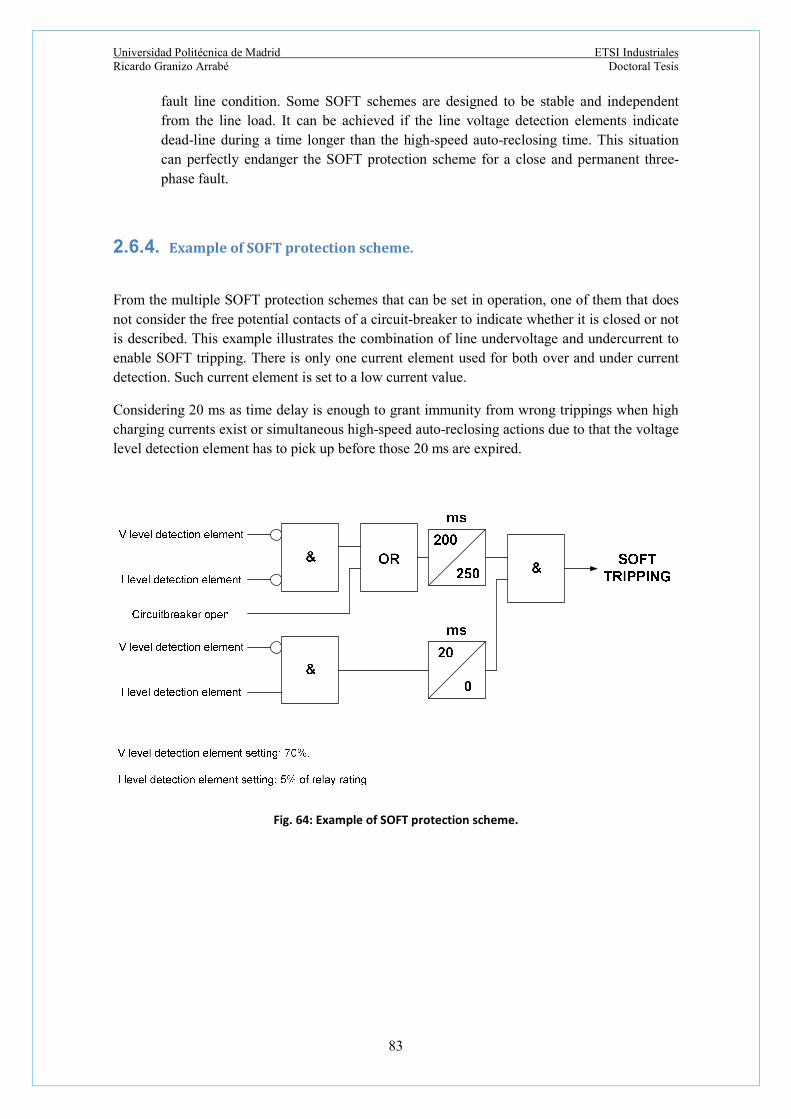
Universidad Politécnica de Madrid ETSI Industriales Ricardo Granizo Arrabé Doctoral Tesis
83
fault line condition. Some SOFT schemes are designed to be stable and independent from the line load. It can be achieved if the line voltage detection elements indicate dead-line during a time longer than the high-speed auto-reclosing time. This situation can perfectly endanger the SOFT protection scheme for a close and permanent three-phase fault.
2.6.4. Example of SOFT protection scheme.
From the multiple SOFT protection schemes that can be set in operation, one of them that does not consider the free potential contacts of a circuit-breaker to indicate whether it is closed or not is described. This example illustrates the combination of line undervoltage and undercurrent to enable SOFT tripping. There is only one current element used for both over and under current detection. Such current element is set to a low current value.
Considering 20 ms as time delay is enough to grant immunity from wrong trippings when high charging currents exist or simultaneous high-speed auto-reclosing actions due to that the voltage level detection element has to pick up before those 20 ms are expired.
Fig. 64: Example of SOFT protection scheme.
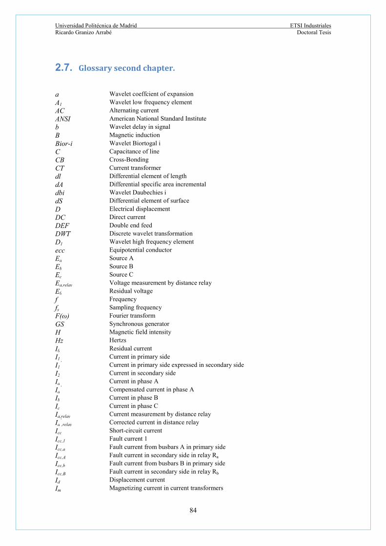
Universidad Politécnica de Madrid ETSI Industriales Ricardo Granizo Arrabé Doctoral Tesis
84
2.7. Glossary second chapter.
a Wavelet coeffcient of expansion A1 Wavelet low frequency element AC Alternating current ANSI American National Standard Institute b Wavelet delay in signal B Magnetic induction Bior-i Wavelet Biortogal i C Capacitance of line CB Cross-Bonding CT Current transformer dl Differential element of length dA Differential specific area incremental dbi Wavelet Daubechies i dS Differential element of surface D Electrical displacement DC Direct current DEF Double end feed DWT Discrete wavelet transformation D1 Wavelet high frequency element ecc Equipotential conductor Ea Source A Eb Source B Ec Source C Ea,relay Voltage measurement by distance relay E0 Residual voltage f Frequency fs Sampling frequency F(ω) Fourier transform GS Synchronous generator H Magnetic field intensity Hz Hertzs I0 Residual current I1 Current in primary side I1
’ Current in primary side expressed in secondary side I2 Current in secondary side Ia Current in phase A Ia
’ Compensated current in phase A Ib Current in phase B Ic Current in phase C Ia,relay Current measurement by distance relay Ia
’,relay Corrected current in distance relay
Icc Short-circuit current Icc,1 Fault current 1 Icc,a Fault current from busbars A in primary side Icc,A Fault current in secondary side in relay Ra
Icc,b Fault current from busbars B in primary side Icc,B Fault current in secondary side in relay Rb
Id Displacement current Im Magnetizing current in current transformers

Universidad Politécnica de Madrid ETSI Industriales Ricardo Granizo Arrabé Doctoral Tesis
85
Ip Maximum value of the steady-state fault current I0 Zero current componente J Electrical current density l Length of line L Inductance of line LA56 Type of aerial conductor La Load A Lb Load B Lc Load C Lm Magnetizing inductance Lbb Total inductance of the burden, leakage resistance and cables from the output
terminal in secondary side of the current transformer LTP Shield voltage limiters m Compensation factor for zero sequence M Wavelet family order MP Mid Point MPL Protection margin level n Turns ratio in current transformer n1 Turns in primary side in current transformer n2 Turns in secundary side in current transformer N Number of turns in a coil NS Number of samples of wavelet coefficients P Indicating factor for protection current transformers Ra Protection relay A. Rb Protection relay B Ri Protection relay i. Rbb Total resistance of the burden, leakage resistance and cables from the output
terminal in secondary side of the current transformer Rcc Core resistance R Correction factor in current transformers RCA Relay characteristic angle R11 Shield resistance R22 Shield resistance S (S-1/2·Ψ(t/S) Wavelet scale factor SEF Single end feed SOFT Switch-on-to-fault SP Single point tRa Time set in protection relay Ra
tRb Time set in protection relay Rb
T Time constant of primary circuit u Induced electromotive force U Threshold value for wavelet analysis Uabsolute Absolute induced voltage Ufw Voltage supported at rated frequency Ulocal Induced voltage Ulw Insulation supported voltage Un Rated voltage for voltage transformers Ur Rated voltage for LPT´s Ures Residual voltage Ut Temporary overvoltage Uu Universal threshold VT Voltage transformer V2 Secondary voltage W Threshold for D1 wavelet components x Fault position

Universidad Politécnica de Madrid ETSI Industriales Ricardo Granizo Arrabé Doctoral Tesis
86
X Value of signal using hard or soft filtering X/R Ratio reactance-resitance in in distribution network YN Star point grounded Z2 Leakage impedance of secundary winding in current transformer Zb Load impedance Zfault Defect impedance Zload Load impedance Zm Magnetizing impedance Zprimary side,ohl Impedance calculated by distance relay expressed in primary side values Zrelay side Impedance calculated by distance relay Zrelay side,errors Impedance calculated by distance relay considering errors Ztotal-burden Total burden impedance Z1,ohl Overhead line impedance ε Error in current transformers θ Inception angle σ Mean of absolute deviation Δt Time difference τ(Ψ(t- τ) Wavelet shift factor λ Flux linkage Φ Magnetic flux
𝜗 Propagation speed
τ Time constant of current transformer φ Angle considering the time constant of the currnt transformer θ Angle of the primary current at steady state μ Magnetic permeability Ψ Mother Wavelet
𝜕𝑡 Differential time incremental
ω Pulsation μ0 Vacuum permeability 1 / √a Wavelet normalization coefficient 52-CB Circuitbreaker

Universidad Politécnica de Madrid ETSI Industriales Ricardo Granizo Arrabé Doctoral Tesis
87

Universidad Politécnica de Madrid ETSI Industriales Ricardo Granizo Arrabé Doctoral Tesis
88
3. STATE OF THE ART IN LOCATION
GROUND FAULTS IN DC POWER SYSTEMS.

Universidad Politécnica de Madrid ETSI Industriales Ricardo Granizo Arrabé Doctoral Tesis
89
his chapter describes the High Voltage Direct Current (HVDC) systems normally used in transmission systems as well as in DC power distribution systems. Again, the circulation of currents in the shields of the power cables is studied, simulated and tested
in laboratory with the aim of finding out new trends to find out new detection methods to locate the ground faults in a selective way.
3.
T

Universidad Politécnica de Madrid ETSI Industriales Ricardo Granizo Arrabé Doctoral Tesis
90
3.1. Introduction to HVDC transmission power systems.
The use of electrical direct current power systems in transmision and distribution is having relevant importance worldwide as there are many new HVDC set in operation year after year.
The neccesity to transport electric energy over long distances, the increasing contribution of renewable energies together with the duty to integrate them into the transmission networks, as well as the development of power electronics, make the use of high voltage direct current an essential complement to traditional AC power systems [83].
HVDC systems employ two different technologies that depend on the type of converter to be installed:
Line Commutated Converter (LCC): this technology uses thyristors as a switching element.
Voltage Source Converter (VSC): this technology has been developed using IGBT´s.
HVDC-VSC technology today is the one that presents the most future prospects for presenting considerable advantages over LCC technology [84].
Nowadays, the development of power electronics has led to the possibility of finding converters at any point in the network where it is necessary to change the form of electric energy (voltage, current or frequency).
Historically, although the first electric distribution networks were operated in direct current, the technology of that time made difficult the implantation of this like standard system of transport of energy, due to the expensive installations and the losses in the conductors. This, together with the advantages of AC transmission, made it possible to widespread the use of AC systems. The improvements in the design of AC generators and the invention of the transformer allowed generating and transporting electricity in a more economical way through HVAC systems. This way, the generation of AC energy very far away from the loads could be done easily.
However, in spite of the advantages that in principle the AC systems provided, with the increase of the transport distances in the HVAC lines, there are problems associated with the reactive reactive energy between the capacitances and the inductances of the systems. However, in HVDC systems, this problem doesn´t exist and the transmission of electrical energy long distances represents no transport losses.
Fig. 65 shows, in a schematic way, the fundamental components of an HVDC system consisting of two HVDC substations where the CA-CC and CC-CA conversions are performed. Therefore two different AC systems are connected. Both conversions can be developed under rectifier mode or as inverter mode in function of the wished power flow direction.

Universidad Politécnica de Madrid ETSI Industriales Ricardo Granizo Arrabé Doctoral Tesis
91
Fig. 65: Basic HVDC system.
3.1.1. Characteristics of HVDC transmission systems.
The use of HVDC´s systems presents several advantages compared to the traditional HVAC systems. The most important are:
Transport distance: HVAC´s systems have transport capacity limitations when the transport distances are long. These problems are mainly related to the capacitances and inductances of the transmission. Every transmission line is characterized by standard electrical parameters as resistance (R), inductive reactance (XL), capacitive reactance (XC) and conductance (G). These parameters are considered as concentrated (short and medium-length lines), or distributed (long-length lines), in order to obtain different equivalent circuits depending on the accuracy required. It is normally accepted that transmission lines are considered in parameters distributed for better accuracy. Comparing the main characteristics of underground cables and overhead conductors, due to the geometry of both, it is observed that the series inductance of the overhead conductors is about 2 to 3 times greater than that of an underground cable. However, the capacitance of an underground cable is in the range of 10 to 20 times greater than the capacitance of an overhead conductor. Therefore, to describe the problem associated with the lengths of lines in HVAC systems, roughly, we can represent the overhead line side as an inductance, and the underground cable line side as a capacity. Following this consideration, the next equivalent schemes are used:
Fig. 66: Current distribution in underground cable.

Universidad Politécnica de Madrid ETSI Industriales Ricardo Granizo Arrabé Doctoral Tesis
92
When an underground power cable is ging to be used, the capacitive current to be charged and discharged must be highly considered. Since the capacity of the cable is proportional to the length of the line, the greater the capacity of the line, the greater the capacitive current required in the charging and discharging of the cable (capacitor). Therefore, for a certain length, called critical length [85], the capacitive current equals the permissible current of the cable, so that all the allowable current would be used to supply the capacitance of the cable, and therefore the cable is unable to be loaded with any single impedance.
Fig. 67: Voltage distribution in overhead conductor.
With the use of overhead conductors, the most important effect is realted to the inductive reactance. If in the case of using an undergrounded cable where its transport capacity was limited due to the absorbed capacitive current, now in the overhead line conductor the limitation is imposed by the voltage drop that occurs in the same. In overhead line conductors as long as the length is bigger, its inductive reactance has bigger values accordingly and the voltage drop across the overhead conductor can make unacceptable the voltage level reached at the load position.
In both cases, the effects of capacitance and inductance can be reduced by means of compensating reactances.
With the use of HVDC lines, the effect of the inductive and capacitive reactance is practically eliminated because the waveforms obtained at the output of the rectifiers contain a low level of ripple [86]. In the ideal case (perfect continuous wave), these effects are completely zero, so theoretically there is no limit of length in the transport of power. Only the resistance must be the parameter to be taken into account in the design of the HVDC line.
Following graph shows the transport capacities in both HVDC and HVAC systems in function of the length of the transmission line.
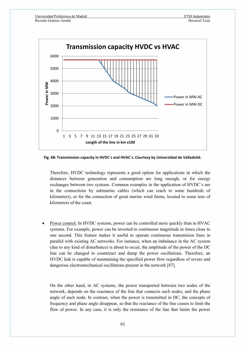
Universidad Politécnica de Madrid ETSI Industriales Ricardo Granizo Arrabé Doctoral Tesis
93
Fig. 68: Transmission capacity in HVDC´s and HVAC´s. Courtesy by Universidad de Valladolid.
Therefore, HVDC technology represents a good option for applications in which the distances between generation and consumption are long enough, or for energy exchanges between two systems. Common examples in the application of HVDC´s are in the connections by submarine cables (which can reach to some hundreds of kilometers), or for the connection of great marine wind farms, located to some tens of kilometers of the coast.
Power control: In HVDC systems, power can be controlled more quickly than in HVAC systems. For example, power can be inverted to continuous magnitude in times close to one second. This feature makes it useful to operate continuous transmision lines in parallel with existing AC networks. For instance, when an imbalance in the AC system (due to any kind of disturbance) is about to occur, the amplitude of the power of the DC line can be changed to counteract and damp the power oscillations. Therefore, an HVDC link is capable of maintaining the specified power flow regardless of severe and dangerous electromechanical oscillations present in the network [87].
On the other hand, in AC systems, the power transported between two nodes of the network, depends on the reactance of the line that connects such nodes, and the phase angle of each node. In contrast, when the power is transmitted in DC, the concepts of frequency and phase angle disappear, so that the reactance of the line ceases to limit the flow of power. In any case, it is only the resistance of the line that limits the power
0
1000
2000
3000
4000
5000
6000
1 3 5 7 9 11 13 15 17 19 21 23 25 27 29 31 33
Pow
er in
MW
Length of the line in km x100
Transmission capacity HVDC vs HVAC
Power in MW-AC
Power in MW-DC

Universidad Politécnica de Madrid ETSI Industriales Ricardo Granizo Arrabé Doctoral Tesis
94
flow. This also means that the power can be transported over long distances by direct current. As an example, two nodes with voltages U1∠δ1 and U2∠δ2, belonging to an
AC network, connected by a line (neglecting their resistance R, and then represented by their reactance jX) are included in the following figure:
Fig. 699: Power flow in AC systems.
The circuit shown before in Fig. 93 can be expressed as:
𝑈 = 𝑈 + 𝑗𝑋. 𝐼 (62)
The current circulating between both nodes is:
𝐼 =𝑈 ∠𝛿 − 𝑈 ∠𝛿
𝑗𝑋=
𝑈 . (𝑐𝑜𝑠𝛿 + 𝑗𝑠𝑒𝑛𝛿 ) − 𝑈 . (𝑐𝑜𝑠𝛿 + 𝑗𝑠𝑒𝑛𝛿 )
𝑗𝑋 (63)
Applying the standard formulas for active power calculation in AC systems, it is obtained:
𝑃 = 𝑅𝑒 𝑈. 𝐼∗ =𝑈 . 𝑈
𝑋. sin(𝛿 − 𝛿 ) (64)
Last expression indicates how the active power transmitted between two nodes depends on the voltages at those nodes, the reactance of the transmission line that joins them, and the difference of angles between the voltages at nodes. Consequently, in long-range transmission lines where the reactance value becomes high, it is necessary and compulsory to carry out a clear compensation to increase the active power transmission capacity. In contrast, in a direct current transmission system, the transmitted active power depends on the value of the voltage at the output of the bridge rectifier, and the current, according to the following figure:

Universidad Politécnica de Madrid ETSI Industriales Ricardo Granizo Arrabé Doctoral Tesis
95
Fig. 700: Power transmission in DC systems.
The power transmitted between nodes 1 and 2 is:
𝑃 = 𝑈 . 𝐼 (65)
Reliability and stability: Any DC link is an asynchronous connection between two alternating current systems that allows interconnecting two systems of different frequencies and phase angles, being for reasons of stability, very difficult or impossible if it were realized in alternating current. They also have the advantage that the disturbances are not transferred from one to another system, or otherwise disturbances in one system do not tend to destabilize the other system. Therefore it is a system that is very useful in case that the generation occurs at variable frequency, as is the case of wind turbines. Meshed AC grids can present problems with high short-circuit currents at times close to the capacity of the installed switchgear. This circumstance is solved with the use of HVDC links since the link to the non-transferring reactive power does not contribute to the increase of the short-circuit power at the connection node.
Economic reasons: The cost of a power transmission line can be divided in two clear costs: one is the cost of investment and the other is the cost of operation and maintenance. From the investment point of view, the following figure shows the investment cost of an electric energy transport facility versus the line length for both DC and AC installations.

Universidad Politécnica de Madrid ETSI Industriales Ricardo Granizo Arrabé Doctoral Tesis
96
Fig. 71: Estimation costs: comparison between HVAC and HVdc power transmission systems. Courtesy by Universidad de Valladolid.
As can be seen, there is therefore a limit from which DC transport is more economical. Logically the limit value depends on the particular conditions of each project (power, technology, etc.). Typically the limit varies from 400 to 700 km in overhead lines and 25 to 50 km in isolated cable lines. The cost of the HVDC substation is much higher than that of the HVAC substation, but the price per km of line is lower in the DC lines, which makes, as just mentioned, that from a certain distance limit, the over-cost of the HVDC substation is compesated. Therefore, DC transmission lines become economically competitive with the AC ones when the length of the line is several hundred kilometres [88]. For example, DC transmission lines demands less number of conductors, the supports and towers to be used may be smaller, and the width of the street may also be smaller, and therefore have a lower environmental impact.
The following figure shows the comparison between an HVAC transmission line and an HVDC one considering the same power to be transmitted:

Universidad Politécnica de Madrid ETSI Industriales Ricardo Granizo Arrabé Doctoral Tesis
97
Fig. 72: HVDC transmission line versus HVAC transmission line. Courtesy by Power Engineers 2009.
From the point of view of the operation, the losses produced must be taken into high consideration. The losses are generally higher in DC lines than in three-phase AC lines. So the losses will be an additional cost for the system. On the other hand, the HVDC systems produce less corona effect than the HVAC lines [89]. From the point of view of maintenance, costs will be reduced in the HVDC lines because they have fewer elements, but higher in the substations due to the need to use converters. In spite of the notable advantages already mentioned [90], the DC transmission power systems present certain disadvantages as:
- The high cost of HVDC substations, compared to AC substations.
- The generation of harmonics in the converters, so that filters have to be installed in order to adapt the voltage and current to the output of these. And thus also be able to ensure an acceptable output side waveform and power factor on the alternating side.
- Electromagnetic fields that interfere with telecommunications may occur due to the harmonics produced by the operations on the converters. These effects can be reduced with the proper use of filters.
- It is not possible to use transformers to change the voltage level.
- In some cases a reactive generator is required.
- Demands complex controls.
- Unlike AC lines, it is not easy to form meshed networks, or to connect new customers at different points along the continuous line, due to the need to coordinate the control of the converters. In fact, continuous lines are usually point-to-point systems, typically from a large generation plant to a large power consumption center. Installing electronic converters at each end of the transmission line, but not intermediate.

Universidad Politécnica de Madrid ETSI Industriales Ricardo Granizo Arrabé Doctoral Tesis
98
3.1.2. HVDC transmission systems: principal network configurations.
The implementation of HVDC networks has different options in function of the distance, soil characteristics and power to be transmitted. The most common network configurations are described in a schematic way [91].
3.1.2.1. HVDC with single pole configuration.
The use of a single-pole configuration in HVDC´s networks has also two options [92]:
3.1.2.1.1. Single-pole HVDC with ground or sea return path.
This system uses a single conductor to drive the electrical energy, making its return by land or by sea using electrodes connected to the converter units. This type of connection is used when the systems to be connected are separated by great distances and where the non-return cable installation can be a considerable saving. It is also used in submarine systems, where the sea performs the return functions, offering fewer losses than a metallic conductor, or when it is not possible to use one of the phases of a bipolar connection. In many cases, existing infrastructure and environmental restrictions prevent the use of return electrodes, as they can lead to corrosion phenomena in nearby facilities. In this case the metallic return is used using a second conductor, in spite of the increase in costs and to generate greater losses.
Fig. 73: HVDC. Single-Pole connection with ground/sea return path.
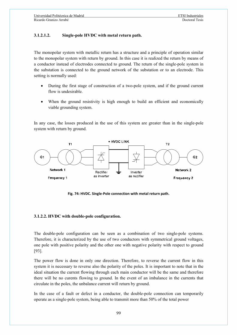
Universidad Politécnica de Madrid ETSI Industriales Ricardo Granizo Arrabé Doctoral Tesis
99
3.1.2.1.2. Single-pole HVDC with metal return path.
The monopolar system with metallic return has a structure and a principle of operation similar to the monopolar system with return by ground. In this case it is realized the return by means of a conductor instead of electrodes connected to ground. The return of the single-pole system in the substation is connected to the ground network of the substation or to an electrode. This setting is normally used:
During the first stage of construction of a two-pole system, and if the ground current flow is undesirable.
When the ground resistivity is high enough to build an efficient and economically viable grounding system.
In any case, the losses produced in the use of this system are greater than in the single-pole system with return by ground.
Fig. 74: HVDC. Single-Pole connection with metal return path.
3.1.2.2. HVDC with double-pole configuration.
The double-pole configuration can be seen as a combination of two single-pole systems. Therefore, it is characterized by the use of two conductors with symmetrical ground voltages, one pole with positive polarity and the other one with negative polarity with respect to ground [93].
The power flow is done in only one direction. Therefore, to reverse the current flow in this system it is necessary to reverse also the polarity of the poles. It is important to note that in the ideal situation the current flowing through each main conductor will be the same and therefore there will be no curents flowing to ground. In the event of an imbalance in the currents that circulate in the poles, the unbalance current will return by ground.
In the case of a fault or defect in a conductor, the double-pole connection can temporarily operate as a single-pole system, being able to transmit more than 50% of the total power

Universidad Politécnica de Madrid ETSI Industriales Ricardo Granizo Arrabé Doctoral Tesis
100
according to the operating criteria and the capacity of the remaining pole, providing greater reliability to the system.
This configuration is used when the carrying capacity of a single-pole link is insufficient, and therefore there is a need for greater power. In addition, the use of a double-pole configuration versus two sibgle-pole systems has the advantage of a lower cost of the line due to the common return, and lower losses.
Within the double-pole configuration there are at least three different alternatives depending on how the return is performed: double-pole with return by ground, double-pole with metallic return and bipolar without return.
3.1.2.2.1. Double-pole HVDC with ground return path.
This configuration provides a high degree of flexibility in its operation, since it can work with a reduced power capacity in case of faults or maintenance of one of its poles, due to the out of service pole (due to fault or maintenance ) can be driven through ground return.
Fig. 75: HVDC. Double-Pole connection with ground return path.
3.1.2.2.2. Double-pole HVDC with metallic ground return path.
The double-pole configuration with metallic return is used when the ground currents are high and the distance between the terminals of the HVDC system is short. It is also used when there is some restriction on the use of electrodes, such as high resistivity of the ground.
In the presence of these conditions, it is necessary to build up the system with a metallic return (either an underground or overhead conductor), so that this conductor can drive the imbalance

Universidad Politécnica de Madrid ETSI Industriales Ricardo Granizo Arrabé Doctoral Tesis
101
currents during the double-pole operation. Likewise, it is also used as a return path when the line of a pole is out of service.
Fig. 76: HVDC: Double-Pole connection with metallic return path.
3.1.2.2.3. Double-pole HVDC without ground return path.
This configuration neither has any electrode nor a return conductor (metallic return). Therefore in case of failure, the mode of operation would be as in a single-pole configuration.
Fig. 77: HVDC: Double-Pole connection without return path.

Universidad Politécnica de Madrid ETSI Industriales Ricardo Granizo Arrabé Doctoral Tesis
102
3.1.2.3. HVDC with homopolar configuration.
This scheme is characterized by the use of two or more cables with the same polarity, usually negative, since it generates fewer losses due to the corona effect. The return can be driven by ground (using electrodes), or metallic (by a conductor) when for technical or environmental reasons ground return can not be used [94].
When there is a fault in a conductor, the complete converter is available for supplying the remaining conductors which, having a certain overload capacity, can carry more than the rated power, reaching up to double depending on the type of connection.
Fig. 78: HVDC: Homopolar connection.
3.1.3. Protections in HVDC transmission power systems.
The protection systems used in HVDC transmission networks must be at least as fast as the protections devices used in HVAC grids or even faster mainly because of the quick developing of high fault currents [95].
The main differences between HVDC and HVAC protection units are based in the different nature of short circuit phenomena. DC fault currents have no zero crossings as AC fault currents and on the other side, DC fault currents reaches their maximum values in extremely low times that implies very fast rising rates [96]. These two main aspects of HVDC fault currents force HVDC protections to eliminate faults very quickly and even faster than HVAC´s and have driven power converters and DC circuit breakers to be used applying different fault clearing strategies. In general in transmission HVDC systems, the protection units currently used are power electronics based as HVDC circuitbreakers or converters that admit only low overcurrent fault values [97].
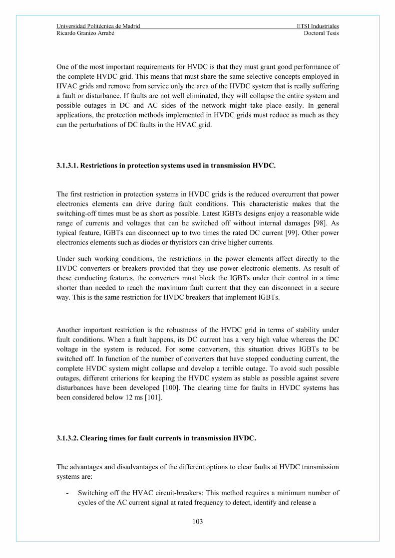
Universidad Politécnica de Madrid ETSI Industriales Ricardo Granizo Arrabé Doctoral Tesis
103
One of the most important requirements for HVDC is that they must grant good performance of the complete HVDC grid. This means that must share the same selective concepts employed in HVAC grids and remove from service only the area of the HVDC system that is really suffering a fault or disturbance. If faults are not well eliminated, they will collapse the entire system and possible outages in DC and AC sides of the network might take place easily. In general applications, the protection methods implemented in HVDC grids must reduce as much as they can the perturbations of DC faults in the HVAC grid.
3.1.3.1. Restrictions in protection systems used in transmission HVDC.
The first restriction in protection systems in HVDC grids is the reduced overcurrent that power electronics elements can drive during fault conditions. This characteristic makes that the switching-off times must be as short as possible. Latest IGBTs designs enjoy a reasonable wide range of currents and voltages that can be switched off without internal damages [98]. As typical feature, IGBTs can disconnect up to two times the rated DC current [99]. Other power electronics elements such as diodes or thyristors can drive higher currents.
Under such working conditions, the restrictions in the power elements affect directly to the HVDC converters or breakers provided that they use power electronic elements. As result of these conducting features, the converters must block the IGBTs under their control in a time shorter than needed to reach the maximum fault current that they can disconnect in a secure way. This is the same restriction for HVDC breakers that implement IGBTs.
Another important restriction is the robustness of the HVDC grid in terms of stability under fault conditions. When a fault happens, its DC current has a very high value whereas the DC voltage in the system is reduced. For some converters, this situation drives IGBTs to be switched off. In function of the number of converters that have stopped conducting current, the complete HVDC system might collapse and develop a terrible outage. To avoid such possible outages, different criterions for keeping the HVDC system as stable as possible against severe disturbances have been developed [100]. The clearing time for faults in HVDC systems has been considered below 12 ms [101].
3.1.3.2. Clearing times for fault currents in transmission HVDC.
The advantages and disadvantages of the different options to clear faults at HVDC transmission systems are:
- Switching off the HVAC circuit-breakers: This method requires a minimum number of cycles of the AC current signal at rated frequency to detect, identify and release a

Universidad Politécnica de Madrid ETSI Industriales Ricardo Granizo Arrabé Doctoral Tesis
104
tripping command to the corresponding circuit-breaker [102]. Unfortunately, this delay time might develop a lack of selectivity in the DC grid.
- Implementation of converters with blocking options: some converters can block fault currents [103]-[104] in the time scale of microseconds with the consequent improvement in fault clearing times respect to the previous method. As drawback it can be said that the complete HVDC grid is removed from service when a fault arises.
- Use of HVDC circuit-breakers: circuit-breakers based on power electronics can switch-off fault currents in times less than 2 ms but have considerable losses in normal operation [105]. Hybrid HVDC circuit-breakers are able to cut fault currents up to 5 ms with reasonable losses [106], [107]. Other option is the use of mechanical circuit-breakers considering a cutting off times about 10 ms, voltages up to 250 kV and fault currents with values in the range of 8 kA [108]. In any case of HVDC circuit-breaker selection, there is a necessity of reducing or limiting the rate of increase of fault currents using normally series inductors with the consequent increase of energy in motion. The installation of those series inductors allows increasing the fault detection and identification or using slow HVDC circuit-breakers.
3.1.3.3. Options for clearing fault currents in transmission HVDC.
There are different options to clear fault currents in transmission HVDCs systems considering the type of power electronics used. Circuit-breakers in combination with protection relays can clear faults seen only at their positions in the grid when the protection relays have no direct communication to other protection relays installed in other positions. If the protection relays can communicate between them, they can clear faults to remove from service the complete protection area for which they are responsible. The most important options are the next ones:
- Local position fault currents cutting-off: when a fault takes place in a transmission line or cable, the fault current is cut by the circuit-breakers installed at both ends. It would be necessary that the clearing time would be lower than the times needed by the converters to reduce the severity of the fault in the entire network. Converters block fault currents in the range of very few milliseconds. Fig. 79 shows the circuit-breakers operation.
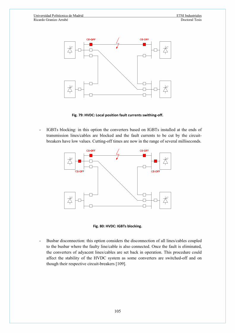
Universidad Politécnica de Madrid ETSI Industriales Ricardo Granizo Arrabé Doctoral Tesis
105
Fig. 79: HVDC: Local position fault currents swithing-off.
- IGBTs blocking: in this option the converters based on IGBTs installed at the ends of transmission lines/cables are blocked and the fault currents to be cut by the circuit-breakers have low values. Cutting-off times are now in the range of several milliseconds.
Fig. 80: HVDC: IGBTs blocking.
- Busbar disconnection: this option considers the disconnection of all lines/cables coupled to the busbar where the faulty line/cable is also connected. Once the fault is eliminated, the converters of adyacent lines/cables are set back in operation. This procedure could affect the stability of the HVDC system as some converters are switched-off and on though their respective circuit-breakers [109].

Universidad Politécnica de Madrid ETSI Industriales Ricardo Granizo Arrabé Doctoral Tesis
106
Fig. 81: HVDC: Busbar diconnection.
- Partial grid disconnection: this option first disconnects the complete area affected by a fault and second isolates the faulty line/cable. Fault clearing times are higher than previous options described.
Fig. 82: HVDC: Partial grid disconnection.
- Complete grid disconnection: this option clears up faults by means of removing from service all converters. Sometimes it is also considered to stablish a maximum fault current level that allows implementing relative slow circuit-breakers and protections and keep part of the HVDC network connected for better stability system.

Universidad Politécnica de Madrid ETSI Industriales Ricardo Granizo Arrabé Doctoral Tesis
107
Fig. 83: HVDC: Complete grid disconnection.
Table 11 includes the different time delays in the protection relays for detection and identification of faults as well as for the fault current cutting-off elements implemented.
Table 11: Time delays in protection relays and methods of fault current cutting-off.
Protection relay Time delay (ms) With communication: 5 - 12 Without communication: 0.1 – 4
Cutting-off elements Time delay (ms) AC circuit-breakers: 33.3/40 Mechanical circuit-breaker: 4 – 12 Hybrid circuit-breaker: 2 - 6 Power electronic circuit-breaker/converter: 0.1
An example of protection zones in HVDCs used for long distance power transmission is illustrated in Fig. 84.

Universidad Politécnica de Madrid ETSI Industriales Ricardo Granizo Arrabé Doctoral Tesis
108
Fig. 84: Protection zones for an HVDC used in long distance power transmission. Courtesy by SIEMENS AG, 2011.
3.1.4. Voltage measurement in HVDC systems.
For the measurement of high DC voltages in HVDC systems, resistive voltage divider type compensation systems (RC dividers) are used. These devices are designed to guarantee a response with a bandwidth ranging from DC to several kHz. Their response must be sufficiently fast to sudden changes in voltage. The output voltage signal will be sent to the protection system to process it individually, either the busbar voltage or the line side voltages. The resistive elements that make up these voltage dividers are basically high-precision, low-inductance resistances, connected in series as a function of the nominal voltage of the network and the value defined for current measurement. In order to protect the RC voltage dividers against resonant phenomena and thus facilitate the wave measurements of the DC voltage or measurements of frequencies with values of some kHz, classification capacitors are also installed connected in parallel to the resistors. The typical response of the RC Dividers shows its little error up to frequencies near 50 kHz in Fig. 85.

Universidad Politécnica de Madrid ETSI Industriales Ricardo Granizo Arrabé Doctoral Tesis
109
0 1 2 3 4 5 6 7 8 9 10
x 105
-2
-1.5
-1
-0.5
0
0.5
1
1.5
2
Frecuencia (Hz)
Fig. 85: HVDC. Divisor RC: Frequency response versus ratio error (%).
This response is much better than that offered by classic voltage transformers, whether inductive or capacitive, since the latter can have errors greater than 100% for frequencies below 2500 Hz. The typical connections of the RC Divisors are shown in the following figure:
Fig. 86: HVDC. Typical connections for a Voltage Divisor RC.

Universidad Politécnica de Madrid ETSI Industriales Ricardo Granizo Arrabé Doctoral Tesis
110
The elements that comprise it are:
R13: primary resistance.
R24: secondary resistance.
F: dielectrical distance.
Rk: load resistance.
C11: primary capacity.
C22: secondary capacity.
Ck: parasitic capacity of the connection cables in secondary.
CB: load resistance.
Some of the main features of RC voltage dividers include:
- High precision achieved in the measure.
- High thermal stability as well as the voltage signal obtained.
- Exact linearity.
- Very short response times.
- Latest generation design technology.
Every RC voltage divider must be designed according to the mechanical and electrical requirements of the HVDC power system in which it is installed. For this reason, it is essential to install or equip the RC voltage divider with terminal boxes (Divider Connection Box). The voltage signals received by these DCB boxes of the RC voltage divider are fully shielded, and depending on the construction models, they are also double shielded. The main mission of the DCB boxes is to transform the intermediate voltage of the RC voltage divider to low amplitude output voltages, the main characteristics of which are the following:
- They can transmit voltage signals over long distances.
- Very precise calibration of the transformation ratio.
- Integral protection against electromagnetic waves.
Furthermore, analogue / digital or analog / Fiber Optic conversion can be carried out in said DCB boxes. These conversions can include as main features:
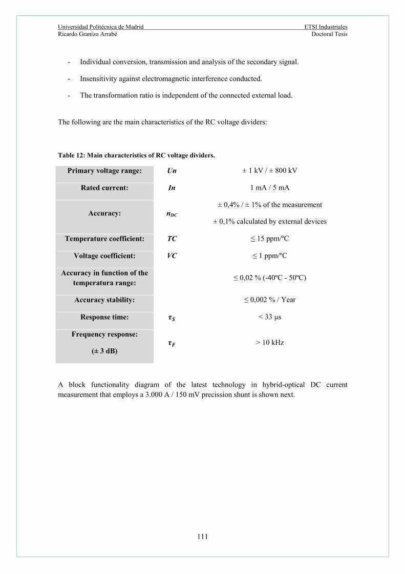
Universidad Politécnica de Madrid ETSI Industriales Ricardo Granizo Arrabé Doctoral Tesis
111
- Individual conversion, transmission and analysis of the secondary signal.
- Insensitivity against electromagnetic interference conducted.
- The transformation ratio is independent of the connected external load.
The following are the main characteristics of the RC voltage dividers:
Table 12: Main characteristics of RC voltage dividers.
Primary voltage range: Un ± 1 kV / ± 800 kV
Rated current: In 1 mA / 5 mA
Accuracy: nDC ± 0,4% / ± 1% of the measurement
± 0,1% calculated by external devices
Temperature coefficient: TC ≤ 15 ppm/ºC
Voltage coefficient: VC ≤ 1 ppm/ºC
Accuracy in function of the temperatura range:
≤ 0,02 % (-40ºC - 50ºC)
Accuracy stability: ≤ 0,002 % / Year
Response time: 𝝉𝑺 < 33 μs
Frequency response:
(± 3 dB) 𝝉𝑭 > 10 kHz
A block functionality diagram of the latest technology in hybrid-optical DC current measurement that employs a 3.000 A / 150 mV precission shunt is shown next.

Universidad Politécnica de Madrid ETSI Industriales Ricardo Granizo Arrabé Doctoral Tesis
112
Fig. 87: Hybrid-Optical DC current measurement. Courtesy by SIEMENS AG, 2011.
3.1.5. Methods for ground fault detection in HVDC networks.
There are different methods for ground fault detection used in HVDC networks. The most widespread methods are described next.
3.1.5.1. Analysis of the initial variation of current di/dt.
This method uses the behaviour of the capacitor at the DC side when a fault happens. A typical equivalent grid is shown in Fig. 88.
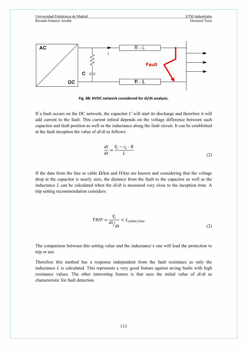
Universidad Politécnica de Madrid ETSI Industriales Ricardo Granizo Arrabé Doctoral Tesis
113
Fig. 88: HVDC network considered for di/dt analysis.
If a fault occurs on the DC network, the capacitor C will start its discharge and therefore it will add current to the fault. This current infeed depends on the voltage difference between such capacitor and fault position as well as the inductance along the fault circuit. It can be established at the fault inception the value of di/dt as follows:
𝑑𝑖
𝑑𝑡=
𝑉 − 𝑖 · 𝑅
𝐿
(2)
If the data from the line or cable Ω/km and H/km are known and considering that the voltage drop at the capacitor is nearly zero, the distance from the fault to the capacitor as well as the inductance L can be calculated when the di/dt is measured very close to the inception time. A trip setting recommendation considers:
𝑇𝑅𝐼𝑃 =𝑉
𝑑𝑖𝑑𝑡
< 𝐿 /
(2)
The comparison between this setting value and the inductance´s one will lead the protection to trip or not.
Therefore this method has a response independent from the fault resistance as only the inductance L is calculated. This represents a very good feature against arcing faults with high resistance values. The other interesting feature is that uses the initial value of di/dt as characteristic for fault detection.

Universidad Politécnica de Madrid ETSI Industriales Ricardo Granizo Arrabé Doctoral Tesis
114
3.1.5.1.1. Fault detection using the rate of current rise.
The use of the rate of current rise to detect faults is mainly due to the quick increase of the current compared to any other working condition as changes in load, switching-oo and on manoeuvres, etc. The key benefit of this kind of detection is that the fault is to be detected lonig time before its maximum fault value is reached. This functionality reduces dramatically the instability created by faults in the HVDC network as well as the breaking capacity for the circuit-breakers to be used. Fig. 89 indicates in an easy way different di/dt zones that can be developed in HVDC systems.
Fig. 89: HVDC: Areas of di/dt for different transients.
3.1.5.2. Analysis of the rate of change of voltage (ROCOV).
This method measures the rate of change of voltage (ROCOV) at the line side in the inductor implemented to limit the di/dt value. The variation in ROCOV´s values can be used as quick fault detection in the range of some microseconds. The differences in ROCOV values allow locating faults in a selective way and discriminate whether the fault has happened in the corresponding protected line, in adyacent lines or at the buses. ROCOV values decrease considerably in function of the distance of the fault to the limiting inductor. The farther the fault occurs, the lower of value of ROCOV. Simulations and research jobs have obtained values for ROCOV over 30.000 kV/ms when a fault happens close to the limiting inductors and and in the range of 1.000 kV/ms for faults at distances over 500 km [110].
The important task is to define the thresholds for indentifying faults within the zone protected or outside it. Therefore, there must be known not only the minimum expected value of ROCOV for a fault inside the protected area that makes the circuit-breakers trip but the maximum expected value of ROCOV for faults outside the protected zone that don´t make the circuit-breakers trip too. These thresholds values are set following an iterative process as the ROCOV depends on the clearing time.
Universidad Politécnica de Madrid ETSI Industriales Ricardo Granizo Arrabé Doctoral Tesis
115
The circuit-breakers installed at different overhead lines and cable lines that feed current to the same fault register different ROCOV values when such fault is cleared. In particular and while a fault is active, the ROCOV values in cable lines that feed such fault decrease. However, during the clearing of the fault ROCOV values will increase.
Bus faults can be detected and idenfied if voltages at both sides of the di/dt limiting inductors are compared. If the change of the voltage in the bus is higher than the change in the voltage in the di/dt limiting inductors, a fault is taking place at the busbars and all circuit-breakers coupled to such busbars must be open. Next formula shows the busbar tripping criteria:
3.1.5.3. Handshaking method.
This method exchanges information between the different HVDC power stations that form VSC´s multiterminal systems (MTDC) [111] to discriminate the zone with defect and isolate it from service in a selective way.
General clearing of faults in the MTDC systems normally are done in first stage by AC circuit-breakers and in second stage by the opening of fast dc switches installed at both line ends.
AC and DC faults show different characteristics and patterns that allow discriminating the fault location:
- AC faults: positive and negative components of the fault currents are normally limited by the VSC´s control whereas the zero components reach high values for ground asymmetrical faults. AC currents at the AC sides of other VSC´s stations present normal operation values. At the DC sides, the VSC´s currents close to the faults develop extensive unbalances with oscillating voltages and currents.
- DC line to line faults: these faults are characterized by having low DC voltage values and extremely high current values. However, at the AC side the values of voltages and currents are low.
- DC line to ground faults: these faults develop DC voltage unbalances and low AC voltages and currents.
𝑑𝑣
𝑑𝑡>
𝑑𝑣
𝑑𝑡
(66)

Universidad Politécnica de Madrid ETSI Industriales Ricardo Granizo Arrabé Doctoral Tesis
116
The next steps describe the functionality of the Handshaking Method:
a. Identification of the possible line with fault: the DC fault current is defined as the difference between the pre-fault and post-fault currents. The direction of the different DC currents through the fast switches inslatted and both ends of the lines of the grid is the relevant information. Once the directions of the DC fault currents are clearly determined, every VSC blocks its respective IGBTs ans selects only the fast dc switch that will be open firstly in the faulted estimated line. The fast dc switch which drives the highest dc fault current is considered to be first one to be open.
b. Fast DC switch opening: once the AC circuit-breakers have been open and the fault current is therefore eliminated, the fast DC switch selected as the first to be open will be open.
c. Charge of DC capacitors: with the faulted line removed from service, AC circuit-breakers are switched-on again and DC capacitors will be charged to their rated values.
d. Closing of fast DC switches: the commands to close the fast DC switches can be released only when the DC line side voltage level is close to the voltage at VSC output terminals.
The process of the Handshaking Method can be implemented in the next terms:
a. Fault detection.
b. VSCs block their IGBTs.
c. Identification of DC faulted line.
d. Open AC circuit-breakers.
e. Delay waiting time to make sure that voltages and currents have zero values.
f. Open fast DC circuit-breakers of the estimated faulted DC line.
g. Delay time to make sure that the VSCs make DC voltage stable again.
h. Close AC circuit-breakers.
i. Close the fast DC switch when voltage levels at both sides reach the value set previously.
j. Set in operation the IGBTs of all VSC sources.

Universidad Politécnica de Madrid ETSI Industriales Ricardo Granizo Arrabé Doctoral Tesis
117
3.1.6. Mechanical DC circuit-breakers.
As result of the development of modular multilevel converters, multiterminal HVDC networks can be a real option for new transmission and distribution power systems where DC circuit breakers have an important role in the protection system [112].
DC circuit-breakers use an LC auxiliary circuit that superimposes an oscillating current on the fault current. This way, a zero crossing current is developed in the fault current path. Such fault current is driven to the loop formed by this auxiliary circuit and will be cleared by the voltage read at another path that has an energy absorber device (MOV). The operation time for DC circuit-breakers is similar to ACs ones. Typical times for the power path are in the range of 15 ms [113]. The use of thyristors as trigger switch in the auxiliary path reduces the total DC circuit-breaker operation time.
Mechanical DC circuit breakers that can interrupt currents up to 16 kA in the range of 8 ms are available in the market [114], [115]. A typical DC circuit-breaker is shown in Fig. 90.
Fig. 90: Typical mechanical DC circuit-breaker structure.
The main elements of a mechanical DC circuit-breaker are:
E: DC voltage source.
C: capacitance for the loop resonant auxiliary circuit.
Idc: DC fault current.
IMOV: residual current in the surge arrester.
IC: charging current.
Imain: current when switch KLC is triggered.

Universidad Politécnica de Madrid ETSI Industriales Ricardo Granizo Arrabé Doctoral Tesis
118
Imech: residual current.
IR: residual current in the isolator switch.
KCB: main circuitbreaker to extinguish the arc.
KLC: switch in the loop resonant auxiliary circuit.
L: inductance for the loop resonant auxiliary circuit.
LDC: limiting reactor of the rate of rise for fault currents.
MOV: surge arrester.
SDC: switch used for cutting the surge arrester leakage current as well as isolating the complete circuit.
When a fault happens, the opening sequence of the mechanical DC circuitbreaker is the next one:
1. Open switch KCB.
2. After the contacts of the switch KCB had reached enough dielectric clearance, close switch KLC.
3. When the current circulating through switch KCB crosses zero value, the current through switch KCB is cut.
4. Fault DC current as well as the current circulating in the auxiliary path LC will be extinguished by measuring the voltage in the surge arresters.
5. Open switch SDC to isolate the leaking current coming from the surge arresters.
6. Activation of charging circuit to set the capacitor voltage in range to be ready for the next cycle.

Universidad Politécnica de Madrid ETSI Industriales Ricardo Granizo Arrabé Doctoral Tesis
119
3.2. Glossary third chapter.
di/dt Current variation in function of time dvbus/dt Variation of bus voltage in function of time dvline-cable/dt Variation of bus voltage in line-cable in function of time DCB Divider connection box G Conductance Gi Voltge source - i HVAC High voltage alternating current HVDC High voltage direct current I Load current IGBT Insulated Gate Bipolar Transistor Io Total load and charging current I0 DC transmission current Ic Charging current IL Short-circuit current in DC system I* Current conjugated L Inductance of line LCC Line commutated converter MTDC Multiterminal DC systems MOV Energy absorber device Pij Active power transmitted from bus i to bus j R Resistance Re Real part of complex number ROCOV Rate of change of voltage U Load voltage UL Overhead voltage drop U0 Rated phase voltage Ui Voltage at bus-i VC DC voltage VSC Voltage source converter XC Capacitive reactance XL Inductive reactance δi Voltage angle at bus-i

Universidad Politécnica de Madrid ETSI Industriales Ricardo Granizo Arrabé Doctoral Tesis
120

Universidad Politécnica de Madrid ETSI Industriales Ricardo Granizo Arrabé Doctoral Tesis
121
4. NEW PROTECTION METHODS FOR AC
POWER SYSTEM
Universidad Politécnica de Madrid ETSI Industriales Ricardo Granizo Arrabé Doctoral Tesis
122
he study of the location of single phase to ground faults is a priority in the responsibilities of the protection relays. Two main research lines have been investigated. The first study is related to the reclosing maneuvers in distribution or transmission
networks and is something to be categorized as a very important issue due to the fatal outcomes that the electrical power system might endure if those autoreclosing orders are given wrongly [80]. Apart from detecting and clearing single phase to ground as quick as possible with selectivity, it is necessary to classify the single phase ground fault at the overhead or cable line side to release or block the autoreclosing maneuver. The most common transmission and distribution systems have been studied, simulated and tested satisfactorily in laboratory. A description of the general equations of cables and shields is given for each case studied.
The second study finds solutions to detect and locate the ground fault in ungrounded networks without using the traditional directional protection functions. Different distribution lay-outs were also simulated and tested and good results were achieved.
T

Universidad Politécnica de Madrid ETSI Industriales Ricardo Granizo Arrabé Doctoral Tesis
123
4.1. Novel method for blocking the auto-reclosing maneouvres in combined overhead-cable lines.
The novel auto-reclosing blocking method for distribution lines that have transitions from overhead to underground cable in distribution systems solidly or impedance grounded with distribution transformers in delta connection in their high voltage sides is introduced in this chapter. The challenge of this new technique is to detect if a ground fault has been produced at the overhead line side or at the cable line side improving the performance of the auto-reclosing functionality. This localization technique is based on the measurements and analysis of the argument differences between the load currents in the active conductors of the cable and the currents in the shields at the cable end where the transformers in delta connection are installed, including a Wavelet analysis of such argument differences.
4.1.1. Combined overhead-cable line with YN and D transformer connections.
This case study applies to distribution lines with overhead and cable sections where the shields of the cables are connected to earth at both ends of the cable and it is known as Single Bonding (SB). No transposition of the cable shields has been implemented.
As example, the composition of any standard cable for medium voltage applications and a flat disposal of three cables are represented in Fig. 91.
Fig. 91: Cable composition (a) and flat disposal (b). (ric) internal conductor radius, (roc) external conductor radius, (ris) internal conductor screen, (ros) external screen radius,(rS) average screen radius,
(SCS) distance between axes of conductor and screen, (tps) external cover thickness.

Universidad Politécnica de Madrid ETSI Industriales Ricardo Granizo Arrabé Doctoral Tesis
124
4.1.2. Impedance of cables and shields.
Self impedances of conductors and shields are evaluated following the Single Bonding connection of shields. Then, the mutual impedances between them are calculated. All impedance calculations follow Carson´s equations considering the effect of the return ground path for all types of self and mutual impedances.
Therefore self impedance of the conductor has the next expression:
ZC = RC(ca) + π2 ·10-7·f + j·4·π·10-7·ln(De/roc) (67)
The expression for the return ground path distance given by Carson is:
De = 1,85··
(6)
On the other hand, the self impedance of the shield has the next expression:
ZS = RS(ca) + π2 ·10-7·f + j·4·π·10-7·ln(De/rs) (69)
The mutual impedance between the conductor “i” and shield “j” can be written as:
ZCS = π2 ·10-7·f + j·4·π·10-7·ln(De/SCS) (70)
In general, the mutual impedance between any conductor and its shield can be written as:
ZCS = π2 ·10-7·f + j·4·π·10-7·ln(De/rS) (71)
The mutual impedance between shields is given by:
ZSS = π2 ·10-7·f + j·4·π·10-7·ln(De/SSS) (72)
4.1.3. Balanced system: General equations for SB shield connections.
The circuit used in the study is shown in Fig. 92 and corresponds with a SB connection.

Universidad Politécnica de Madrid ETSI Industriales Ricardo Granizo Arrabé Doctoral Tesis
125
Fig. 92: Standard shields connection for SB applications. (Ia, Ib, Ic) Currents in Conductors,( Isa, Isb, Isc)
Currents in Shields, (R1, R2) Ground Resistances at both ends of shields, (U) Voltage Difference between shield terminals.
When the load currents form a three-phase balanced system and only positive sequence component exists, the vector sum of the line currents flowing in the conductors is zero. The voltages induced in screens have a component due to the flow of current through conductor, and another due to the currents circulating in the screens. As shown in the previous figure, the screens are connected at both ends to ground and voltages between the two grounding connections are equal to the three screens and it can be expressed as:
U = U1C + U1S = U2C + U2S = U3C + U3S (73)
The mathematical models for such induced voltages are listed below:
- Induced voltages in shields due to circulating currents in conductors:
U1C = L·(ZC1S1·I1 + ZC2S1·I2 + ZC3S1·I3)
U2C = L·(ZC1S2·I1 + ZC2S2·I2 + ZC3S2·I3)
U3C = L·(ZC1S3·I1 + ZC2S3·I2 + ZC3S3·I3)
(74)

Universidad Politécnica de Madrid ETSI Industriales Ricardo Granizo Arrabé Doctoral Tesis
126
- Induced voltages in shields due to circulating currents in shields:
U1S = L·(ZS1S1·IS1 + ZS2S1·IS2 + ZS3S1·IS3)
U2S = L·(ZS1S2·IS1 + ZS2S2·IS2 + ZS3S2·IS3)
U3S = L·(ZS1S3·IS1 + ZS2S3·IS2 + ZS3S3·IS3)
(75)
All previous equations can be expressed in a matrix system:
S
S
S
C
C
C
U
U
U
U
U
U
U
U
U
3
2
1
3
2
1
3
2
1
(76)
Where:
3
2
1
333231
232221
131211
3
2
1
333231
232221
131211
3
2
1
····
S
S
S
SSSSSS
SSSSSS
SSSSSS
SCSCSC
SCSCSC
SCSCSC
I
I
I
ZZZ
ZZZ
ZZZ
L
I
I
I
ZZZ
ZZZ
ZZZ
L
U
U
U
(77)
4.1.4. Principles of the Novel Auto-Reclosing Blocking Method for Distribution
Networks.
The new method investigated in this job measures the currents at the three shields of the cables at their end located at the substation side and the currents in the active part of the three phase of the cable as it is indicated in Fig. 93. It has been studied for solidly or low value impedance grounded power distribution networks with distribution transformers in delta connection at their high voltage sides. It employs a trigger signal to start its analysis and has been considered a total time signal length to be evaluated of 40 ms as pre-trigger time and 40 ms active fault time. This trigger signal is provided by any protection relay when a ground fault has been detected. The time set 40 ms for active fault time is acceptable as the ground faults at distribution networks are active longer times and the minimum tripping time for standard overcurrent or voltage relays is 30 ms. Apart from this time, the medium voltage circuit-breaker opening times are not less than 40-50 ms. That means that the time of 40 ms as active fault time has turned out to be good enough as it will be seen in the simulation and real tests results.

Universidad Politécnica de Madrid ETSI Industriales Ricardo Granizo Arrabé Doctoral Tesis
127
Once this trigger signal has been acknowledged, the new method initiates the procedure to classify where the ground fault has happened and takes the decision whether to block or not the reclosing maneuver. With the shields connected in SB disposal, the new method first evaluates the angle difference between the currents in the active part of the cables and their corresponding shields during 80 ms, 40 ms as pre-trigger time and 40 ms as active fault time. This angle difference is indicated from now on as ΔL1S1, ΔL2S2 and ΔL3S3 for the respective phases and corresponding shields. A second evaluation is developed to have second decision criteria and make sure that the right maneuver will be taken up. This second evaluation is a wavelet analysis of those angle differences. The wavelet analysis uses the discrete wavelet transform (DWT) and evaluates only the high frequency elements [116], [117]. These two analyses are described next.
Fig. 93: Currents measured of the cables in the active conductors and in their shields.
4.1.4.1. Analysis of the angle differences between currents in conductors and currents in
shields.
This analysis evaluates the angle differences ΔL1S1, ΔL2S2 and ΔL3S3. In normal operation without ground fault, the currents circulating in staggered cables in the three shields form a balanced system and the angle differences between active currents and shield currents have the similar values. Cables in flat disposal enjoy unbalanced currents in shields as the distance between all them are not exactily the same between each others whereas cables in delta disposal normally have very similar currents. In function of the ground fault position, the phase-shield currents angle differences are increased, decreased or keep the angle difference values Their behaviour allow in most cases identifying where the ground fault has happened.

Universidad Politécnica de Madrid ETSI Industriales Ricardo Granizo Arrabé Doctoral Tesis
128
Typical overhead lines up to 30 km and cable lengths up to 1.200 m have been evaluated as a case study. However this method could be used in similar configurations with larger distances.
When the ground fault happens in the overhead side, the currents in the shields are due to the mutual coupling between all conductors and shields. In such ground fault conditions, the angle difference between them has values in the range between 50º and 100º approximately. Practically all ground fault current circulates from the fault point to the grounding system in the main distribution substation which power transformer is grounded.
But if the ground fault happens in the cable side, ground fault current circulates from the fault point to both ends of the shield of the phase with defect. The shield of the cable with ground defect acts as a ground fault current divider. At the earthing of such shield at both cable ends, both defect currents return to the main substation whereas the currents circulating in the shields of the phases without defect, keep their circulating from one end to the other of the cable. This circulation process makes that ΔL1S1, ΔL2S2 and ΔL3S3 are increased in a great deal. The threshold to decide if the auto-reclosing maneouvre is blocked has been selected in 50º and it appears in the algorithm developed for this new application.
In this research, Daubechies 2 mother wavelet, db2, has been selected as it has good characteristics to classify the magnitude of D1 component when the ground fault is located at the overhead or at the cable side of the line. The threshold for D1 value components has been selected to 50 to block the auto-reclosing order when its value is higher. The variable W represents its value in the algorithm as it can be seen in Fig. 94.
4.1.4.2. Algorithm of the new auto-reclosing blocking method.
In Fig. 94 it is shown the algorithm used to determine where the ground fault is. The analysis of ΔL1S1, ΔL2S2 and ΔL3S3 is developed in parallel with a wavelet analysis that evaluates the maximum values of the dB2 - cD1 coefficients for such ΔL1S1, ΔL2S2 and ΔL3S3. These values of the dB2 – cD1 coefficients are analyzed and the variable W is obtained.

Universidad Politécnica de Madrid ETSI Industriales Ricardo Granizo Arrabé Doctoral Tesis
129
Fig. 94: Algorithm of the new auto-reclosing method.
4.1.4.3. Simulation results: analysis.
The proposed new auto reclosing blocking method was simulated using Simulink® in a typical distribution network presented as a case study. An equivalent “pi” model for lines was used as well as power transformers rated 66/20 kV, 20 MVA with Dyn1 connection group and distribution transformers rated 20/0,4 kV, 630 kVA and connection group Dyn11. Loads in these distribution transformers have been consider up to 600 kVA with standard power factors from 0.85 inductive to 1. The grid scheme used has one overhead distribution line with a total length of 24 km. The “pi” parameters of the overhead line without ground wire have the next values: R0=0.831 Ω/km; R1=0.687 Ω/km; L0=0.00486 H/km; L1=L2=0.001383 H/km; C0=4.24·10-9 F/km; C1=C2=8.89·10-9 F/km. The conductor type is LA-56 with diameter ΦLA56=9.45 mm, RLA56=0.616 Ω/km; Imax=199.35 A and geometric mean distance GMD=2.53 m. The underground cable used is RHZ1 2OL 12/20 kV which main features are: ΦCable-
core=13.82mm, Sc=150 mm2, Ss= 16 mm2, R=0.188 Ω/km, Φext=34.4 mm. It has been chosen a cable length from 600 to 1.200 m. The shields of these cables are connected in SB whereas the overhead line considers span lengths of 100 m. The ground resistance at the transition has considered a typical value of 12 Ω and at the cable end substation 0,5 Ω. The model used is indicated in Fig. 95.

Universidad Politécnica de Madrid ETSI Industriales Ricardo Granizo Arrabé Doctoral Tesis
130
Fig. 95: New auto-reclosing blocking method: Model implemented.
Continuous
powergui
VoltagesSubstation BVoltages
Substation A
NABC
Un=66 kVScc=1500MVA
A
B
C
a
b
c
n2
Transformer: ST=630kVA
UT=20/0.4 kVDyn11
A
B
C
a
b
c
n2
TransformerST=20 MVAUT=66/20 kV
Dyn1Vabc
IabcA
B
C
a
b
c
Three-PhaseV-I Measurement3
Vabc
IabcA
B
C
a
b
c
Three-PhaseV-I Measurement1
VabcIabc
A
B
C
abc
Three-PhaseV-I Measurement
Substation B
Vabc
IabcA
B
C
a
b
c
Three-PhaseV-I Measurement
Substation A
Shield Voltages Substation B
Shield Currents Substation B
Rt
Rdefect1Rdefect
R3
R1
R 66 kV
ABC
ABC
Overhead Line12 km
ABC
ABC
Overhead Line12 km
Load currents
Load Voltages
ABC
Load400kVA
CurrentsSubstation A
Conductor CurrentsSubstation B
Breaker - L: Fault at Overhead SideBreaker - C: Fault at Cable Side
Cable 1
screen 1
Cable 2
screen 2
Cable 3
screen 3
Cable 1
screen 1
Cable 2
screen 2
Cable 3
screen 3
B: 3 Cables connection SB
Cable 1
screen 1
Cable 2
screen 2
Cable 3
screen 3
Cable 1
screen 1
Cable 2
screen 2
Cable 3
screen 3
A: 3 Cables connection SB

Universidad Politécnica de Madrid Ricardo Granizo Arrabé
131
4.1.4.4. Angle Difference Analysis in Distribution Networks Solidly Grounded at the
Overhead Side and Isolated at the Cable End Side
The angle differences ΔL1S1, ΔL2S2 and ΔL3S3 between currents in the shields and in the active part of the cables in a system ungrounded at the cable side (typical power transformer in delta connection) and solidly grounded at the overhead side is simulated. Multiple simulations show that the classification of the ground faults turns out to be:
- Ground fault in overhead side: if ΔL1S1, ΔL2S2 and ΔL3S3 are less than 50º normally in all phases.
- Ground fault in the cable side: if at least one ΔL1S1, ΔL2S2 or ΔL3S3 is clearly over 50º.
Fig. 96 and 97 show ΔL1S1, ΔL2S2 and ΔL3S3 when there is a ground fault in phase L1 at the overhead side at 12 km from the transition and at the cable side in its central position in t=200 ms. The overhead has a total length of 24 km and the cable 600 m.
Fig. 966: Angle differences with ground fault at the overhead side in phase L1.
0.15 0.2 0.25 0.3-100
-95
-90
-85
-80
-75
-70
-65
-60
Time (s)
An
gle
Diff
ere
nce
Co
ndu
ctor
-Sh
ield
(d
egr
ee
s)
Ground fault in t=200 ms at the overhead side in phase L1
Angle difference L1-S1Angle Difference L2-S2Angle Difference S3-L3 15,64º
12,20º 15,44º

Universidad Politécnica de Madrid ETSI Industriales Ricardo Granizo Arrabé Doctoral Tesis
132
Fig. 97: Angle differences with ground fault at the cable side in phase L1.
Considering distances from the transition, Tables 13 and 14 show the results of the change in ΔL1S1, ΔL2S2 and ΔL3S3 from only 1 m to more than 10 km in the overhead side and from only 1 m to 599 m in the cable side also.
0.15 0.2 0.25 0.3-400
-300
-200
-100
0
100
Time (s)
An
gle
Diff
ere
nce
Pha
se-S
hie
ld (
deg
ree
s)
Ground fault in t=200 ms at the cable side in phase L1
Angle Difference L1-S1Angle Difference L2-S2Angle Difference L3-S3
167,95º
73,35º23,15º

Universidad Politécnica de Madrid ETSI Industriales Ricardo Granizo Arrabé Doctoral Tesis
133
Table 12: Phase angle variation after with ground faults at the overhead and cable sides.
FAULT AT OVERHEAD SIDE FAULT AT CABLE SIDE
Distance from
transition
Fault in phase L1
Distance from
transition
Fault in phase L1
Change in angles Change in angles
ΔL1S1 ΔL2S2 ΔL3S3 ΔL1S1 ΔL2S2 ΔL3S3
1 m 15.18º 10.98º 15.26º 1 m 73.69º 168.62º 24.03º
10 m 15.16º 10.99º 15.24º 10 m 73.72º 168.65º 24.05º
100 m 15.17º 11.01º 15.26º 50 m 73.75º 168.61º 24.12º
1.000 m 15.18º 11.05º 14.27º 100 m 73.71º 168.52º 23.73º
5.000 m 15.25º 11.33º 15.37º 300 m 73.35º 167.95º 23.15º
>10.000 m 15.44º 12.20º 15.64º 599 m 72.75º 6.45º 131.11º
FAULT AT OVERHEAD SIDE FAULT AT CABLE SIDE
Distance from
transition
Fault in phase L2
Distance from
transition
Fault in phase L2
Change in angles Change in angles
ΔL1S1 ΔL2S2 ΔL3S3 ΔL1S1 ΔL2S2 ΔL3S3
1 m 15.34º 15.33º 10.81º 1 m 24.02º 73.72º 168.58º
10 m 15.35º 15.34º 10.88º 10 m 24.10º 73.70º 168.59º
100 m 15.34º 15.33º 10.87º 50 m 23.92º 73.71º 168.47º
1.000 m 15.37º 15.36º 10.85º 100 m 23.85º 73.79º 168.42º
5.000 m 15.48º 15.45º 11.20º 300 m 22.99º 73.55º 167.65º
>10.000 m 15.67º 15.56º 11.72º 599 m 131.08º 72.74º 6.90º

Universidad Politécnica de Madrid ETSI Industriales Ricardo Granizo Arrabé Doctoral Tesis
134
Table 13: Phase angle variation after with ground faults at the overhead and cable sides.
FAULT AT OVERHEAD SIDE FAULT AT CABLE SIDE
Distance from
transition
Fault in phase L3
Distance from
transition
Fault in phase L3
Change in angles Change in angles
ΔL1S1 ΔL2S2 ΔL3S3 ΔL1S1 ΔL2S2 ΔL3S3
1 m 11.78º 15.41º 15.25º 1 m 168.61º 24.01º 73.31º
10 m 11.79º 15.42º 15.22º 10 m 168.62º 24.02º 73.70º
100 m 11.77º 15.43º 15.23º 50 m 168.51º 23.92 73.72º
1.000 m 11.82º 15.45º 15.25º 100 m 168.40º 23.75º 73.31º
5.000 m 12.13º 15.55º 15.33º 300 m 168.12º 23.11º 73.55º
>10.000 m 12.66º 15.73º 15.45º 599 m 6.76º 131.42º 72.78º
4.1.4.5. Wavelet Analysis in a Distribution System Solidly Grounded at the Overhead Side
and Isolated at the Cable End Side.
The simulation results of this configuration show that the angle difference when the ground fault has happened in the overhead side has dB2 - cD1 coefficients lower than 0.1 and over 100 when the fault is in the cable side. Next two figures show such results.
Fig. 98: Wavelet dB2-1 - cD1 coefficients of the angle differences signals with ground fault in phase L1 at the overhead side 12 km from the transition.
0.1995 0.2 0.2005 0.201 0.2015-0.2
-0.15
-0.1
-0.05
0
0.05
0.1
0.15
0.2
Time (s)
dB
2-c
D1
Co
eff
icie
nts
Ground fault in t=0.2 s at the overhead side in phase L1
cD1 Angle difference Conductor L2/Shield L2cD1 Angle difference Conductor L3/Shield L3cD1 Angle difference Conductor L1/Shield L1

Universidad Politécnica de Madrid ETSI Industriales Ricardo Granizo Arrabé Doctoral Tesis
135
Fig. 99: Wavelet db2-1 - cD1 coefficients of the angle differences signals with ground fault in phase L1 at the cable side 300 m from the transition.
Table 14: Wavelet analysis: simulation results. Ground faults at the overhead and cable sides. Overhead side solidly grounded and cable side isolated. Phase currents measured in the conductors (L1, L2, L3) and in their shields (S1, S2, S3).
FAULT AT OVERHEAD SIDE FAULT AT CABLE SIDE
Distance from
transition
Fault in phase L1
Distance from
transition
Fault in phase L1
W (dB2 – cD1 coefficients) W (dB2 – cD1 coefficients)
ΔL1S1 ΔL2S2 ΔL3S3 ΔL1S1 ΔL2S2 ΔL3S3
1 m 0.0068 0.0067 0.0065 1 m 173.88 0.0134 0.0096
10 m 0.0039 0.0041 0.0041 10 m 173.89 0.0123 0.0097
100 m 0.0033 0.0038 0.0039 50 m 127.32 0.0113 0.0094
1.000 m 0.0027 0.0029 0.0025 100 m 127.32 0.0119 0.0097
5.000 m 0.0019 0.0024 0.0019 300 m 127.31 0.0128 0.0089
>10.000 m 0.0014 0.0016 0.0013 599 m 123.67 0.02784 0.0332
0.18 0.185 0.19 0.195 0.2 0.205
0
50
100
150
Time (s)
dB
2-c
D1
Co
eff
icie
nts
db2-cD1 Coefficioents for ground fault in the the cable side in t=0.2 s in phase L1
cD1-Angle Difference Conductor L2/Shield S2cD1-Angle Difference Conductor L1/Shield S1cD1-Angle Difference Conductor L3/Shield S3
127.3
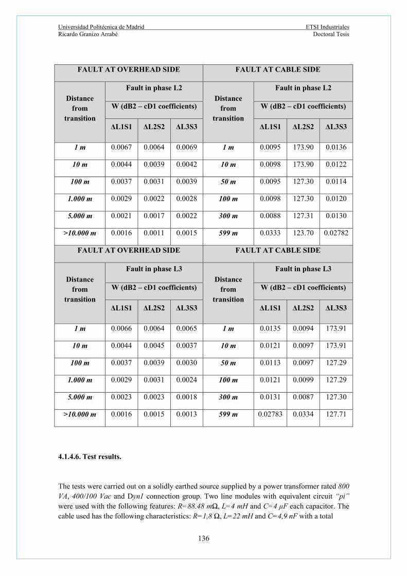
Universidad Politécnica de Madrid ETSI Industriales Ricardo Granizo Arrabé Doctoral Tesis
136
FAULT AT OVERHEAD SIDE FAULT AT CABLE SIDE
Distance from
transition
Fault in phase L2
Distance from
transition
Fault in phase L2
W (dB2 – cD1 coefficients) W (dB2 – cD1 coefficients)
ΔL1S1 ΔL2S2 ΔL3S3 ΔL1S1 ΔL2S2 ΔL3S3
1 m 0.0067 0.0064 0.0069 1 m 0.0095 173.90 0.0136
10 m 0.0044 0.0039 0.0042 10 m 0.0098 173.90 0.0122
100 m 0.0037 0.0031 0.0039 50 m 0.0095 127.30 0.0114
1.000 m 0.0029 0.0022 0.0028 100 m 0.0098 127.30 0.0120
5.000 m 0.0021 0.0017 0.0022 300 m 0.0088 127.31 0.0130
>10.000 m 0.0016 0.0011 0.0015 599 m 0.0333 123.70 0.02782
FAULT AT OVERHEAD SIDE FAULT AT CABLE SIDE
Distance from
transition
Fault in phase L3
Distance from
transition
Fault in phase L3
W (dB2 – cD1 coefficients) W (dB2 – cD1 coefficients)
ΔL1S1 ΔL2S2 ΔL3S3 ΔL1S1 ΔL2S2 ΔL3S3
1 m 0.0066 0.0064 0.0065 1 m 0.0135 0.0094 173.91
10 m 0.0044 0.0045 0.0037 10 m 0.0121 0.0097 173.91
100 m 0.0037 0.0039 0.0030 50 m 0.0113 0.0097 127.29
1.000 m 0.0029 0.0031 0.0024 100 m 0.0121 0.0099 127.29
5.000 m 0.0023 0.0023 0.0018 300 m 0.0131 0.0087 127.30
>10.000 m 0.0016 0.0015 0.0013 599 m 0.02783 0.0334 127.71
4.1.4.6. Test results.
The tests were carried out on a solidly earthed source supplied by a power transformer rated 800 VA, 400/100 Vac and Dyn1 connection group. Two line modules with equivalent circuit “pi” were used with the following features: R=88.48 mΩ, L=4 mH and C=4 μF each capacitor. The cable used has the following characteristics: R=1,8 Ω, L=22 mH and C=4,9 nF with a total

Universidad Politécnica de Madrid ETSI Industriales Ricardo Granizo Arrabé Doctoral Tesis
137
cable length of 300 m. Two overcurrent protection relays type MRI4 by Woodward-Seg are used as disturbance recorder to store the values of the currents flowing in the active conductors and in the shields of the cables. A second transformer rated 800 VA, 400/100 Vac and Dyn11 is used to supply different loads in delta connection. Fig. 100 includes the experimental set-up and the RLC features of the line modules used.
Fig. 100: Experimental set-up. (1: Protection relays; 2: Auxiliary power supply; 3: Power supply; 4: Loads; 5: Ground defect switch; 6: Transformer; 7: PC; 8: Cables; 9: Line modules; 10: Line module box;
11: RLC parameters of the line modules used).
Several single ground defects at all phases in lines and in cables were carried out in the network erected in the laboratory. Tests were developed at 100 V phase-to-phase voltage and load currents less than 1 A with different cosφ values. The positions where the ground defects were developed are represented in a schematic way in Fig. 101.

Universidad Politécnica de Madrid ETSI Industriales Ricardo Granizo Arrabé Doctoral Tesis
138
Fig. 101: Ground defect positions: (A: at the end of the cable, B: between first and second section of the cables; C: between the second and third section of the cables; D: in the transition at the end of the
cables; E: between the first and second tram of the line modules; F: behind the two line modules).
Fig. 102: Ground defect positions: schematic representation.

Universidad Politécnica de Madrid ETSI Industriales Ricardo Granizo Arrabé Doctoral Tesis
139
4.1.4.7. Angle Analysis of the Experimental Distribution System Solidly Grounded at the
Overhead Side and Isolated at the Cable End Side.
The angle differences ΔL1S1, ΔL2S2 and ΔL3S3 obtained in the tests in a system ungrounded at the cable and solidly grounded at the overhead side turn out to be:
- Ground fault in overhead side: if the angle difference between the active and respective shield of the currents in the phase with defect is less than 50º.
- Ground fault in the cable side: if the angle difference between the active and respective shield of the currents in the phase with defect is clearly over 50º.
Fig. 103 shows the angle difference between phase and shield currents when there is a ground fault in phase L1 in the overhead side at fault point E and at the cable side in fault point C.
Fig. 103: Angle differences with ground fault at the overhead side in phase L1. Fault point E.
Tables 16, 17 and 18 show the results of ΔL1S1, ΔL2S2 and ΔL3S3 in ground fault locations A, B, C, D in the cable side, and in locations E and F at the overhead side.
0.2 0.25 0.3 0.35 0.4 0.45 0.5-160
-140
-120
-100
-80
-60
-40
-20
Time (s)
Deg
ree
s (º
)
Angle change between currents in conductors and shields.Ground fault at the overhead side in E.
Angle difference Conductor L1/Shield S1Angle difference Conductor L3/Shield S3Angle difference Conductor L2/Shield S2
32.3º
27.2º30.8º

Universidad Politécnica de Madrid ETSI Industriales Ricardo Granizo Arrabé Doctoral Tesis
140
Fig. 104: Angle differences with ground fault at the cable side in phase L1. Fault point C.
Table 15: Ground fault at overhead and cable sides in phase L1. Change in angles between currents in the conductors and their respective shields.
FAULT AT CABLE SIDE
PLACE OF THE FAULT
Fault in Phase L1
Change in angles
ΔL1S1 ΔL2S2 ΔL3S3
A 66.32º 11.02º 0.33º
B 65.93º 10.24º 0.26º
C 64.89º 9.82º 0.20º
D 64.25º 9.31º 0.18º
FAULT AT OVERHEAD SIDE
PLACE OF THE FAULT
Fault in Phase L1
Change in angles
ΔL1S1 ΔL2S2 ΔL3S3
E 30.80 32.31 27.16
F 29.12 31.86 26.02
0.12 0.14 0.16 0.18 0.2 0.22 0.24 0.26 0.28 0.3-400
-350
-300
-250
-200
-150
-100
-50
Time (s)
De
gre
es
(º)
Angle difference between currents in conductors and shieldswith ground fault in cable side in phase L1
Angle difference Conductor L1 / Shield S1Angle difference Conductor L2 / Shield S2Angle difference Conductor L3 / Shield S3
9.82º
64.89º
0.2º

Universidad Politécnica de Madrid ETSI Industriales Ricardo Granizo Arrabé Doctoral Tesis
141
Table 16: Ground fault at overhead and cable sides in phase L2. Change in angles between currents in the conductors and their respective shields.
FAULT AT CABLE SIDE
PLACE OF THE FAULT
Fault in Phase L2
Change in angles
ΔL1S1 ΔL2S2 ΔL3S3
A 0.29º 66.45º 12.08º
B 0.25º 65.99º 10.93º
C 0.21º 65.02º 9.88º
D 0.16º 64.67º 9.33º
FAULT AT OVERHEAD SIDE
PLACE OF THE FAULT
Fault in Phase L2
Change in angles
ΔL1S1 ΔL2S2 ΔL3S3
E 1.29 31.78 16.29
F 1.11 25.11 12.11

Universidad Politécnica de Madrid ETSI Industriales Ricardo Granizo Arrabé Doctoral Tesis
142
Table 17: Ground fault at overhead and cable sides in phase L3. Change in angles between currents in the conductors and their respective shields.
FAULT AT CABLE SIDE
PLACE OF THE FAULT
Fault in Phase L3
Change in angles
ΔL1S1 ΔL2S2 ΔL3S3
A 12.58º 0.30º 67.34º
B 10.13º 0.26º 66.86º
C 9.01º 0.20º 65.78º
D 8.92º 0.18º 64.02º
FAULT AT OVERHEAD SIDE
PLACE OF THE FAULT
Fault in Phase L3
Change in angles
ΔL1S1 ΔL2S2 ΔL3S3
E 17.34 1.35 32.45
F 14.22 1.18 23.67
4.1.4.8. Wavelet Analysis of the Experimental Distribution System Solidly Grounded at the
Overhead Side and Isolated at the Cable End Side.
The cD1 coefficients obtained from the angle differences in the tests between currents in the shields and in the active cables in a system ungrounded at the cable and solidly grounded at the overhead side turned out to be:
- Ground fault in overhead side: if the cD1 coefficients values have lower values than 50 in all phases.
- Ground fault in the cable side: if the cD1 coefficients values have values much more higher than 50, in the range of 100 or more.

Universidad Politécnica de Madrid ETSI Industriales Ricardo Granizo Arrabé Doctoral Tesis
143
Fig. 105 shows the dB2 – cD1 coefficient values of the angle difference between phase and shield currents when there is a ground fault in phase L1 in the overhead side at fault point E whereas Fig. 106 shows the dB2 – cD1 coefficient values of the angle difference between phase and shield currents when there is a ground fault in phase L1 at the cable side in fault point C.
Fig. 105: Wavelet analysis of the angle differences with ground fault at the overhead side in phase L1. Fault point E.
Fig. 106: Wavelet analysis of the angle differences with ground fault at the overhead side in phase L1. Fault point C.
0.08 0.085 0.09 0.095 0.1 0.105 0.11
-6
-4
-2
0
2
4
Time (s)
dB
2-c
D1
Coe
ffic
ien
ts
dB2-cD1 Coefficients for ground fault in phase L1 at the overhead side in position E
dB2-cD1 coefficients Conductor L1 / Shield S1dB2-cD1 coefficients Conductor L2 / Shield S2dB2-cD1 coefficients Conductor L3 / Shield S3
0.030.5
4.8
0.15 0.16 0.17 0.18 0.19 0.2 0.21 0.22-160
-140
-120
-100
-80
-60
-40
-20
0
20
Time (s)
dB
b2
-cD
1 C
oeff
icie
nt V
alu
es
dB2-cD1 Coefficient values for ground fault in phase L1 at the cable side in location C
dB2-cD1 Coeffientes Conductor L1 / Shield S1dB2-cD1 Coeffientes Conductor L2 / Shield S2dB2-cD1 Coeffientes Conductor L3 / Shield S3
142
0.8 7.2

Universidad Politécnica de Madrid ETSI Industriales Ricardo Granizo Arrabé Doctoral Tesis
144
Table 18: Ground fault at overhead and cable sides. Wavelet analysis: experimental results. Overhead side solidly grounded and cable side isolated.
FAULT AT CABLE SIDE FAULT AT OVERHEAD SIDE
Location of the fault
Fault in phase L1
Location of the fault
Fault in phase L1
W (dB2 – cD1 coefficients) W (dB2 – cD1 coefficients)
ΔL1S1 ΔL2S2 ΔL3S3 ΔL1S1 ΔL2S2 ΔL3S3
A 152.24 2.45 18.29 E 4.80 0.03 0.50
B 145.88 1.96 14.12
C 142.01 0.80 7.21 F 4.66 0.02 0.42
D 136.54 0.69 4.75
FAULT AT CABLE SIDE FAULT AT OVERHEAD SIDE
Location of the fault
Fault in phase L2
Location of the fault
Fault in phase L2
W (dB2 – cD1 coefficients) W (dB2 – cD1 coefficients)
ΔL1S1 ΔL2S2 ΔL3S3 ΔL1S1 ΔL2S2 ΔL3S3
A 20.04 154.31 3.01 E 0.04 4.88 0.59
B 16.59 148.22 2.42
C 9.92 143.67 0.89 F 0.03 4.72 0.48
D 6.82 138.08 0.82
FAULT AT CABLE SIDE FAULT AT OVERHEAD SIDE
Location of the fault
Fault in phase L3
Location of the fault
Fault in phase L3
W (dB2 – cD1 coefficients) W (dB2 – cD1 coefficients)
ΔL1S1 ΔL2S2 ΔL3S3 ΔL1S1 ΔL2S2 ΔL3S3
A 2.66 19.44 153.01 E 0.47 0.04 4.34
B 1.49 15.18 144.78
C 0.81 6.96 140.12 F 0.51 0.02 4.11
D 0.52 3.97 134.96

Universidad Politécnica de Madrid ETSI Industriales Ricardo Granizo Arrabé Doctoral Tesis
145
4.1.4.9. Conclusions.
A new auto-reclosing blocking method for distribution lines which have transitions overhead to underground cable side has been presented in this research. The shields of the cables are connected to earth at both ends. The proposed ground fault auto-reclosing method is based on two analyses. The first one evaluates the argument difference between the currents in the active part of the cable and the currents in the shields whereas the second analysis uses the wavelet Daubechies dB2 and extracts the coefficients cD1 from the same argument differences used in the first analysis. If the argument differences between the currents in the conductor of the cable and the currents in the shields have a phase variation just after a ground fault happens with higher values than a reference argument difference and, at the same time, the Daubechies - cD1 coefficients of such argument differences have values over a reference threshold, it is determined that the ground fault has happened in the cable side and the reclosing is blocked. On the other hand, if the phase variation just after a ground fault takes place between the currents in the conductor of the cable and the currents in the shields have lower values than a reference argument difference and, at the same time, the Daubechies - cD1 coefficients of such argument differences have very small values, it is determined that the ground fault has happened at the overhead side and the reclosing is released.
Simulations turned out to be totally satisfactory and the experimental results of the laboratory tests showed that the localization of the ground fault is correct. This novel technique has important advantages when compared to up and running ground fault detection systems:
It discriminates if a ground fault happens at the overhead or cable side.
It does not use any voltage measurement.
It does not use any directional criterion
It does not use the residual ground fault current to localize the ground fault.
It does not consider any distance calculation to localize the ground fault.
It does not consider any differential tripping criterion to localize the ground fault.
The aforementioned advantages of the proposed technique make easier to determine where the ground fault is, and consequently, allow to the protection relay making the best possible use of the auto-reclosing functionality. The stability of the grid is also improved as wrong reclosing commands are not sent while ground faults conditions are active. This research will continue with the evaluation of this new method in networks with other grounding systems with different cable and shield connections.

Universidad Politécnica de Madrid ETSI Industriales Ricardo Granizo Arrabé Doctoral Tesis
146
4.2. Novel Protection Method for Detection of ground Faults in Cables Used
in Combined Overhead-Cable Lines in Power Systems
Power transmission systems use protection relays to detect and clear different types of faults as soon as possible with total selectivity in order to minimize damages in the power elements that form the electrical power network as well as to reduce the instability in the network caused by such faults. In those systems that supply important loads like cities or factories, there are many overhead-cable transition stations that supply those loads. Some transmission lines have two different parts, one is the underground cable side and the other one is the overhead side [118], [119]. Protection systems must be accurate in order to be able to locate ground faults. Protection systems applied to overhead lines are different from the principles employed in cable protection systems [120]. It is very important that the clearance time of the fault is less than the time needed to drive the system to an irrecoverable instability [121]. Protection systems installed to protect combined overhead-cable lines are totally able to detect and clear any type of fault but they do not know if the fault happened at the overhead-line side or at the cable line side. Transmission lines rated 220 or 400 kV normally have three protection relays installed at each end: line differential as primary protection whereas distance and ground fault directional overcurrent are the back-up protections. In this way, if the transmission line is overhead type, after a ground fault had been cleared up, the reclosing order will be released. On the other hand, if the transmission line is cable type, after a ground fault had been eliminated, the reclosing order will be blocked. This research presents a new cable protection technique to be used in combined overhead-cable lines in the range of 50 km that connects big substations around consume areas to substations inside those consume areas like big cities or important industrial areas. This technique allows determining if a ground fault has taken place in the cable line side or not. The two end substations are solidly grounded and the shields of the cables are connected according the cross-bonding method. Standard EN60909-3 [122] for impedance calculation has been considered in the models developed. Fig. 107 shows a typical transmission network with some overhead lines and one overhead-cable line.

Universidad Politécnica de Madrid ETSI Industriales Ricardo Granizo Arrabé Doctoral Tesis
147
Fig. 107: Transmission system with overhead-cable transition station. (1) Active conductor of Power Cables, (2) Shields of the Power-Cable, (Rt) Tower Ground Resistance, (Rsa) Ground Resistance of
Substation – A, (Rsb) Ground Resistance of Substation – B.
4.2.1. Principles of operation.
This method compares the currents in the shields as illustrated in Fig. 109. In function of the differences in magnitude and phase between them, the method distinguishes the location of the ground fault. If the magnitude differences are less than a threshold K, the ground fault is identified as fault outside the cable line side. But if the magnitude differences are higher than such threshold K, the ground fault is identified as fault inside the cable line side. The other comparison is related to the phase angle difference of those currents. If the phase differences between all them are less than a threshold P, the fault is considered to have occurred outside the cable line side. However, if the phase differences between all them are greater than threshold P, the fault is located at the cable line side. The new method considers both coefficients M and P to discriminate the position of the ground fault.
Only when both coefficients indicate that the fault has happened in the cable line side, a tripping command indication is released to switch off the combined overhead – cable line at both ends.
However, when the ground fault occurs very close to the transition, cable or overhead side,
the analysis described before is not sufficient to make sure that the cable has the fault.
Therefore, the currents measured in the shields are analyzed in a different way. A covariance calculation between the values of those currents circulating in the shields and their respective angles is developed. If the covariance has a value higher than 0.2, the ground fault is

Universidad Politécnica de Madrid ETSI Industriales Ricardo Granizo Arrabé Doctoral Tesis
148
in the cable. But if its value is lower than 0.2, the ground fault is outside the cable. The algorithm developed is shown in Fig. 108.
Fig. 108: Algorithm proposed.

Universidad Politécnica de Madrid ETSI Industriales Ricardo Granizo Arrabé Doctoral Tesis
149
Fig. 109: Measurement of consductor and shield currents.
4.2.2. Simulation results.
The proposed cable protection was simulated as a case study using Simulink® considering the data of a real network in Madrid area. An equivalent model for short lines of less than 50 km was used. Overhead line side substation has a shortcircuit power Scc-3phase=13269.34 MVA with X/R=9.84 whereas the substation at the cable line end has a shortcircuit power Scc-
3phase=12479.42 MVA with X/R=9.5. Loads at 220 kV busbars have been considered up to 50 MVA with standard power factors from 0.85 inductive to 1. The grid scheme used has one overhead transmission line with a total length of 1481 m and cable line with 2688 m. The parameters of the overhead line with one ground wire type have the next values: R0=0.22438 Ω/km; R1=0.12008 Ω/km; L0=0.00314 H/km; L1=L2=0.001446 H/km; C0=5.0644·10-9 F/km; C1=C2=7.9731·10-9 F/km. The conductor type is LA-280 Hawk with diameter ΦLA280=21.8 mm, RLA280=0.1194 Ω/km; Imax=579 A and geometric mean distance GMD=12.25 m. The ground wire type is AC-50 with diameter ΦAC50=9 mm and RLA50=4.095 Ω/km. The underground cable used is XLPE 127/220 kV 1x1200 AL which main features are: ΦCable-conductor=43.6 mm, Sconductor=1200 mm2, Sshield= 95 mm2, Rconductor=0.0151 Ω/km, Φext-cable=114.5 mm. The cable has three sections with lengths of 894, 897 and 897 m each one. The shields of these cables are connected in CB arrangement whereas the overhead line considers span lengths of 230 m. The ground resistance at the transition has considered a typical value of 12 Ω and at the cable end substation 0,5 Ω. The model used is indicated in Fig. 110. Ground fault resistances have been considered from 0.1 to 30 Ω as well as different fault angles inception.

Universidad Politécnica de Madrid ETSI Industriales Ricardo Granizo Arrabé Doctoral Tesis
150
Fig. 110: Simulation for ground fault analysis.
Continuous
powergui
Transition U-I
N
A
B
C
Sub.BUn=220kV
N
A
B
C
Sub.AUn=220kV Shields U-I
R6
R4R3
Phases U-I
Overhead line
Conn1
Conn3
Conn5
Conn7
Conn9
Conn11
Conn2
Conn4
Conn6
Conn8
Conn10
Conn12
Measurements inShields
Vabc
IabcA
B
C
a
b
c
M3
Vabc
IabcA
B
C
a
b
c
M2
Vabc
IabcA
B
C
a
b
c
M1
Vabc
IabcA
B
C
a
b
c
M
Grid U-I
Cable 1
screen 1
Cable 2
screen 2
Cable 3
screen 3
Cable 1
screen 1
Cable 2
screen 2
Cable 3
screen 3
Cable
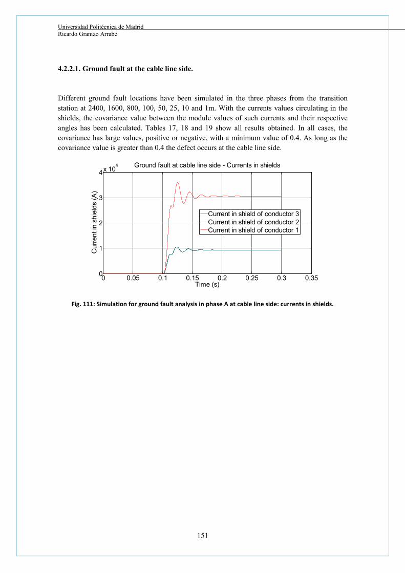
Universidad Politécnica de Madrid Ricardo Granizo Arrabé
151
4.2.2.1. Ground fault at the cable line side.
Different ground fault locations have been simulated in the three phases from the transition station at 2400, 1600, 800, 100, 50, 25, 10 and 1m. With the currents values circulating in the shields, the covariance value between the module values of such currents and their respective angles has been calculated. Tables 17, 18 and 19 show all results obtained. In all cases, the covariance has large values, positive or negative, with a minimum value of 0.4. As long as the covariance value is greater than 0.4 the defect occurs at the cable line side.
Fig. 111: Simulation for ground fault analysis in phase A at cable line side: currents in shields.
0 0.05 0.1 0.15 0.2 0.25 0.3 0.350
1
2
3
4x 10⁴
Time (s)
Cur
rent
in s
hiel
ds (
A)
Ground fault at cable line side - Currents in shields
Current in shield of conductor 3Current in shield of conductor 2Current in shield of conductor 1
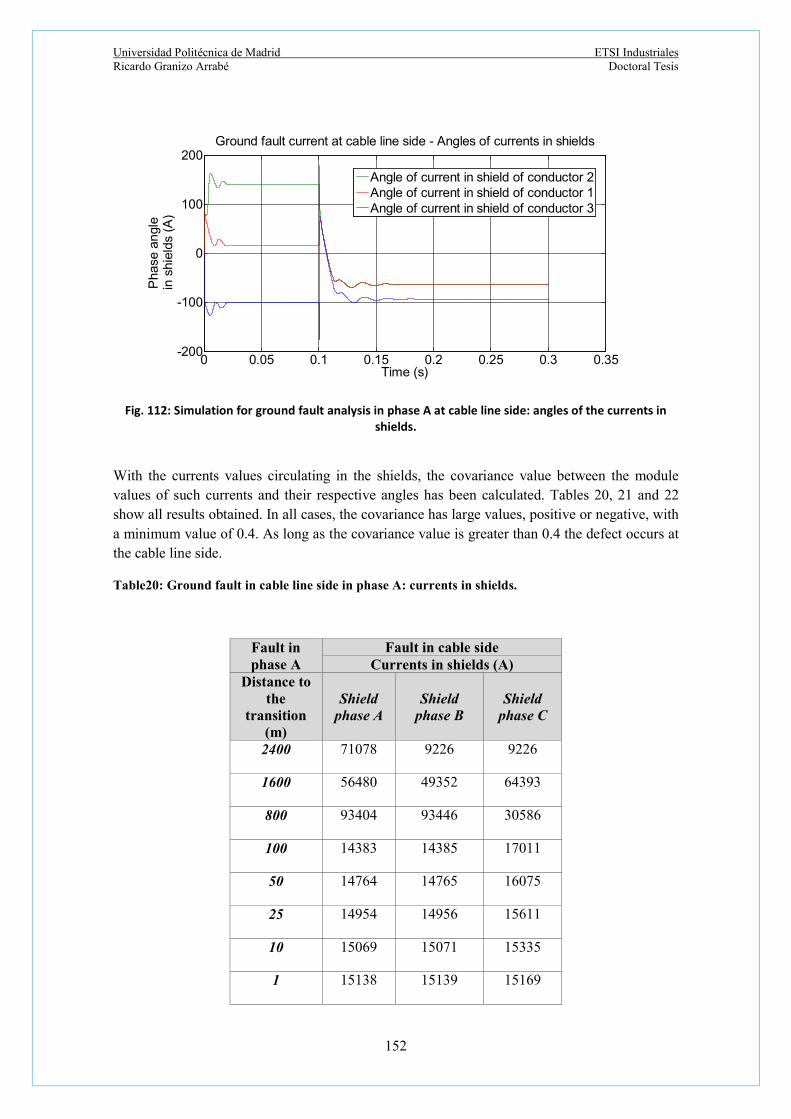
Universidad Politécnica de Madrid ETSI Industriales Ricardo Granizo Arrabé Doctoral Tesis
152
Fig. 112: Simulation for ground fault analysis in phase A at cable line side: angles of the currents in shields.
With the currents values circulating in the shields, the covariance value between the module values of such currents and their respective angles has been calculated. Tables 20, 21 and 22 show all results obtained. In all cases, the covariance has large values, positive or negative, with a minimum value of 0.4. As long as the covariance value is greater than 0.4 the defect occurs at the cable line side.
Table20: Ground fault in cable line side in phase A: currents in shields.
Fault in phase A
Fault in cable side Currents in shields (A)
Distance to the
transition (m)
Shield phase A
Shield phase B
Shield phase C
2400 71078 9226 9226
1600 56480 49352 64393
800 93404 93446 30586
100 14383 14385 17011
50 14764 14765 16075
25 14954 14956 15611
10 15069 15071 15335
1 15138 15139 15169
0 0.05 0.1 0.15 0.2 0.25 0.3 0.35-200
-100
0
100
200
Time (s)
Pha
se a
ngl
ein
shi
elds
(A
)
Ground fault current at cable line side - Angles of currents in shields
Angle of current in shield of conductor 2Angle of current in shield of conductor 1Angle of current in shield of conductor 3

Universidad Politécnica de Madrid ETSI Industriales Ricardo Granizo Arrabé Doctoral Tesis
153
Table 19: Ground fault in cable line side in phase B: currents in shields.
Fault in phase B
Fault in cable side Currents in shields (A)
Distance to the
transition (m)
Shield phase A
Shield phase B
Shield phase C
2400 9240,41 70415 9240,01
1600 6502,11 5595,92 49112
800 30484 9275,52 9279,71
100 16922 14299 14301
50 15986 14677 14679
25 15522 14866 14868
10 15245 14980 14982
1 15080 15048 15050
Table 20: Ground fault in cable line side in phase C: currents in shields.
Fault in phase C
Fault in cable side Currents in shields (A)
Distance to the
transition (m)
Shield phase A
Shield phase B
Shield phase C
2400 9232,41 9232,82 72019
1600 49819 6486,81 5626,42
800 9393,61 30877 9389,52
100 14506 17169 14504
50 14893 16222 14892
25 15088 15753 15086
10 15205 15473 15203
1 15275 15305 15273
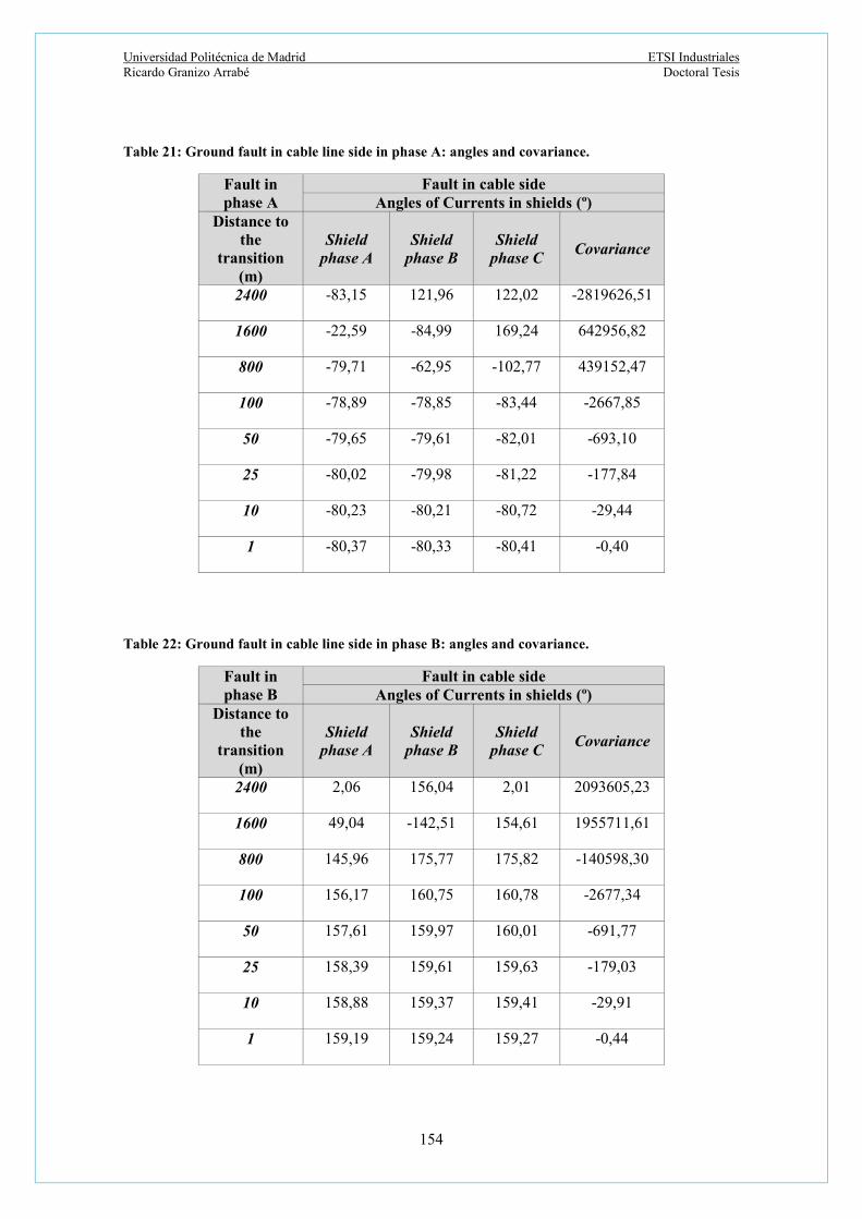
Universidad Politécnica de Madrid ETSI Industriales Ricardo Granizo Arrabé Doctoral Tesis
154
Table 21: Ground fault in cable line side in phase A: angles and covariance.
Fault in phase A
Fault in cable side Angles of Currents in shields (º)
Distance to the
transition (m)
Shield phase A
Shield phase B
Shield phase C
Covariance
2400 -83,15 121,96 122,02 -2819626,51
1600 -22,59 -84,99 169,24 642956,82
800 -79,71 -62,95 -102,77 439152,47
100 -78,89 -78,85 -83,44 -2667,85
50 -79,65 -79,61 -82,01 -693,10
25 -80,02 -79,98 -81,22 -177,84
10 -80,23 -80,21 -80,72 -29,44
1 -80,37 -80,33 -80,41 -0,40
Table 22: Ground fault in cable line side in phase B: angles and covariance.
Fault in phase B
Fault in cable side Angles of Currents in shields (º)
Distance to the
transition (m)
Shield phase A
Shield phase B
Shield phase C
Covariance
2400 2,06 156,04 2,01 2093605,23
1600 49,04 -142,51 154,61 1955711,61
800 145,96 175,77 175,82 -140598,30
100 156,17 160,75 160,78 -2677,34
50 157,61 159,97 160,01 -691,77
25 158,39 159,61 159,63 -179,03
10 158,88 159,37 159,41 -29,91
1 159,19 159,24 159,27 -0,44
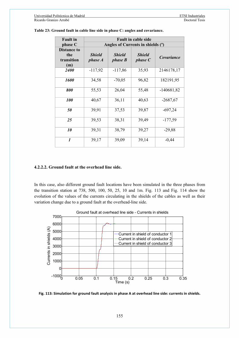
Universidad Politécnica de Madrid ETSI Industriales Ricardo Granizo Arrabé Doctoral Tesis
155
Table 23: Ground fault in cable line side in phase C: angles and covariance.
Fault in phase C
Fault in cable side Angles of Currents in shields (º)
Distance to the
transition (m)
Shield phase A
Shield phase B
Shield phase C
Covariance
2400 -117,92 -117,86 35,93 2146178,17
1600 34,58 -70,05 96,82 182191,95
800 55,53 26,04 55,48 -140681,82
100 40,67 36,11 40,63 -2687,67
50 39,91 37,53 39,87 -697,24
25 39,53 38,31 39,49 -177,59
10 39,31 38,79 39,27 -29,88
1 39,17 39,09 39,14 -0,44
4.2.2.2. Ground fault at the overhead line side.
In this case, also different ground fault locations have been simulated in the three phases from the transition station at 738, 500, 100, 50, 25, 10 and 1m. Fig. 113 and Fig. 114 show the evolution of the values of the currents circulating in the shields of the cables as well as their variation change due to a ground fault at the overhead-line side.
Fig. 113: Simulation for ground fault analysis in phase A at overhead line side: currents in shields.
0 0.05 0.1 0.15 0.2 0.25 0.3 0.35-1000
0
1000
2000
3000
4000
5000
6000
7000
Time (s)
Cu
rren
ts in
sh
ield
s (A
)
Ground fault at overhead line side - Currents in shields
Current in shield of conductor 1Current in shield of conductor 2Current in shield of conductor 3

Universidad Politécnica de Madrid ETSI Industriales Ricardo Granizo Arrabé Doctoral Tesis
156
Fig. 114: Simulation for ground fault analysis in phase A at overhead line side: angles of the currents in shields.
With the currents values circulating in the shields, the covariance value between the module values of such currents and their respective angles has again been calculated. Tables 23, 24 and 25 show all results obtained.
Table 24: Ground fault at overhead line side in phase A: currents in shields.
Fault in phase A Fault at overhead side
Currents in shields (A) Distance to the transition (m)
Shield phase A Shield phase B Shield phase C
738 6006,22 6015,41 6010,31
500 5709,11 5718,42 5712,91
250 5389,32 5398,81 5392,92
100 5323,22 5332,71 5326,73
50 5311,42 5320,91 5314,92
25 5306,91 5316,42 5310,33
10 5304,11 5313,62 5307,63
1 5303,68 5312,02 5305,98
0 0.05 0.1 0.15 0.2 0.25 0.3 0.35-200
-100
0
100
200
Time (s)
Ang
le o
f cu
rre
nts
in s
hiel
ds
Ground fault at overhead line side - Angles of currents in shields
Angle of current in shield of conductor 2Angle of current in shield of conductor 1Angle of current in shield of conductor 3

Universidad Politécnica de Madrid ETSI Industriales Ricardo Granizo Arrabé Doctoral Tesis
157
Table 25: Ground fault at overhead line side in phase B: currents in shields.
Fault in phase B Fault at overhead side
Currents in shields (A) Distance to the transition (m)
Shield phase A Shield phase B Shield phase C
738 6026,91 6022,92 6032,01
500 5632,11 5628,31 5637,72
250 5401,21 5397,72 5407,02
100 5333,01 5329,52 5339,01
50 5320,32 5316,91 5326,42
25 5315,71 5312,31 5321,93
10 5313,31 5308,78 5318,88
1 5312,54 5308,11 5316,45
Table 26: Ground fault at overhead line side in phase C: currents in shields.
Fault in phase C Fault at overhead side
Currents in shields (A) Distance to the transition (m)
Shield phase A Shield phase B Shield phase C
738 6056,32 6051,11 6047,12
500 5661,21 5657,51 5661,83
250 5429,82 5423,91 5420,33
100 5361,31 5355,24 5351,72
50 5344,61 5343,53 5342,01
25 5341,82 5339,88 5337,22
10 5341,11 5335,32 5331,48
1 5340,66 5334,39 5329,94

Universidad Politécnica de Madrid ETSI Industriales Ricardo Granizo Arrabé Doctoral Tesis
158
Tables 26, 27 and 28 show all results obtained. In all cases, the covariance has values lower than 0.1, positive or negative, with a maximum value of 0.096. As long as the covariance value is lower than 0.1 the defect occurs at the overhead line side.
Table 27: Ground fault at overhead line side in phase A: angles and covariance.
Fault in phase A
Fault at overhead side Angles of Currents in shields (º)
Distance to the
transition (m)
Shield phase A
Shield phase B
Shield phase C
Covariance
738 -22,14 -22,12 -22,21 0,040
500 -18,99 -18,98 -19,08 0,034
250 -16,04 -16,03 -16,13 0,040
100 -14,97 -14,96 -15,06 0,042
50 -14,66 -14,66 -14,76 0,028
25 -14,52 -14,51 -14,61 0,044
10 -14,44 -14,43 -14,54 0,045
1 -14,36 -14,35 -14,41 0,037
Table 28: Ground fault at overhead line side in phase B: angles and covariance.
Fault in phase B
Fault at overhead side Angles of Currents in shields (º)
Distance to the
transition (m)
Shield phase A
Shield phase B
Shield phase C
Covariance
738 -142,03 -141,95 -141,94 0,026
500 -138,42 -138,33 -138,32 0,035
250 -135,95 -135,86 -135,85 0,040
100 -134,89 -134,81 -134,79 0,057
50 -134,59 -134,49 -134,49 0,030
25 -134,45 -134,35 -134,34 0,049
10 -134,24 -134,16 -134,11 0,096
1 -134,02 -133,98 -133,99 -0,016

Universidad Politécnica de Madrid ETSI Industriales Ricardo Granizo Arrabé Doctoral Tesis
159
Table 29: Ground fault at overhead line side in phase C: angles and covariance.
Fault in phase C
Fault at overhead side Angles of Currents in shields (º)
Distance to the
transition (m)
Shield phase A
Shield phase B
Shield phase C
Covariance
738 98,33 98,23 98,31 0,043
500 101,95 101,85 101,94 0,084
250 104,41 104,31 104,41 0,026
100 105,46 105,36 105,45 0,043
50 105,61 105,65 105,75 -0,062
25 105,76 105,79 105,82 -0,046
10 105,96 105,99 106,02 -0,096
1 106,28 106,23 106,24 0,078
4.2.3. Experimental results.
In order to give evidence of the simulations results, different laboratory tests have been developed to verify the validity of the proposed new cable protection method.
4.2.3.1. Experimental set-up.
The tests were carried out on a network with two sources solidly earthed supplied by two power transformers rated 800 VA, 400/100 Vac and Dyn1 connection group. Two line modules with equivalent circuit “pi” have been used with the following characteristics: R=88.48 mΩ, L=4 mH and C=4 μF each capacitor. The cable used has the following characteristics: R=1,8 Ω, L=22 mH and C=4,9 nF with a total cable length of 300 m. One overcurrent protection relay type MRI4 by Woodward-Seg is used as disturbance recorder to store the values of the currents flowing in the shields of the cables. Different single ground defects at every phase in lines and in cables were performed. All tests were developed at 100 V phase-to-phase voltage and load currents less than 1 A with different cosφ values. The positions where the ground defects were developed are represented in a schematic way in Fig. 115.

Universidad Politécnica de Madrid ETSI Industriales Ricardo Granizo Arrabé Doctoral Tesis
160
CURRENTRELAY
SHIELDS
SHIELDS
CABLE SECTIONSLINE MODULES
SOURCE
AC BF E D
R-L
C C
TRANSFORMER
LOAD
TRANSFORMER
LOAD
SOURCE
Fig. 115: Ground defect positions: schematic representation.

Universidad Politécnica de Madrid Ricardo Granizo Arrabé
161
4.2.3.2. Ground fault at the cable line side.
The tests results for ground faults in the cable in the three phases in locations D-E-F are listed in Table 29. It can be observed that covariance values get higher values from ground faults close to the transition in location D to ground faults at the end of the cable in location F. Those values are included in Table 30.
Table 30: Ground fault in cable side: currents in shields.
Fault in location D
Fault in cable side Currents in shields (A)
Shield phase A Shield phase B Shield phase C
Phase A 1,17 3,07 1,16
Phase B 1,06 1,08 3,44
Phase C 3,06 1,24 1,25
Fault in location E
Fault in cable side
Currents in shields (A)
Shield phase A Shield phase B Shield phase C
Phase A 7,14 0,38 0,96
Phase B 0,91 7,23 0,42
Phase C 0,46 1,01 6,45
Fault in location
F
Fault in cable side
Currents in shields (A)
Shield phase A Shield phase B Shield phase C
Phase A 1,09 1,04 62,92
Phase B 62,89 1,08 1,04
Phase C 1,12 62,92 1,03

Universidad Politécnica de Madrid ETSI Industriales Ricardo Granizo Arrabé Doctoral Tesis
162
Table 31: Ground fault in cable side: angles and covariance of currents in shields.
Fault in location D
Fault in cable side
Angles of currents in shields (A) Covariance
Shield phase A Shield phase B Shield phase C
Phase A 131,92 92,48 133,41 -17,014
Phase B -35,16 -32,91 -78,45 -23,384
Phase C 23,96 58,01 56,35 -13,402
Fault in location E
Fault in cable side
Angles of currents in shields (A) Covariance
Shield phase A Shield phase B Shield phase C
Phase A 38,81 67,82 92,18 -56,867
Phase B 81,49 26,87 62,19 -64,030
Phase C -7,10 14,28 -38,49 -51,482
Fault in location
F
Fault in cable side
Angles of currents in shields (A) Covariance
Shield phase A Shield phase A Shield phase A
Phase A -51,81 -50,91 99,84 2078,321
Phase B -51,78 -50,92 99,84 -1048,543
Phase C 161,86 -44,65 164,87 -2858,865
4.2.3.3. Ground fault at overhead line side.
Now the tests results for ground faults at the overhead line side in the three phases in locations A-B-C are listed in Table 31. It can be observed that in these cases, the covariance values are meaningless when defects happen along the overhead as listed in Table 32.

Universidad Politécnica de Madrid ETSI Industriales Ricardo Granizo Arrabé Doctoral Tesis
163
Table 32: Ground fault at overhead side: currents in shields.
Fault in location A
Fault in cable side Currents in shields (A)
Shield phase A Shield phase B Shield phase C
Phase A 1,25 1,21 1,24
Phase B 1,24 1,22 1,26
Phase C 1,30 1,20 1,20
Fault in location B
Fault in cable side
Currents in shields (A)
Shield phase A Shield phase B Shield phase C
Phase A 1,21 1,17 1,21
Phase B 1,21 1,21 1,24
Phase C 1,31 1,17 1,19
Fault in location
C
Fault in cable side
Currents in shields (A)
Shield phase A Shield phase B Shield phase C
Phase A 1,61 1,57 1,61
Phase B 1,57 1,59 1,64
Phase C 1,81 1,60 1,62

Universidad Politécnica de Madrid ETSI Industriales Ricardo Granizo Arrabé Doctoral Tesis
164
Table 33: Ground fault at overhead side: angles and covariance of currents in shields.
Fault in location A
Fault in cable side
Angles of currents in shields (A) Covariance
Shield phase A Shield phase B Shield phase C
Phase A 174,11 174,21 174,32 0,000
Phase B 136,77 136,66 136,38 -0,002
Phase C -152,81 -150,86 -151,25 -0,039
Fault in location B
Fault in cable side
Angles of currents in shields (A) Covariance
Shield phase A Shield phase B Shield phase C
Phase A 40,38 41,27 41,63 -0,002
Phase B 180,10 179,90 179,90 -0,001
Phase C -23,21 -24,42 -25,73 0,050
Fault in location
C
Fault in cable side
Angles of currents in shields (A) Covariance
Shield phase A Shield phase A Shield phase A
Phase A 20,57 21,51 21,93 -0,002
Phase B -53,20 -50,63 -50,07 0,033
Phase C -86,44 -87,71 -89,18 0,084
4.2.3.4. Conclusions.
Simulation and laboratory test results show that ground faults in short combined overhead-cable lines that occur at the cable line side can be perfectly detected if comparisons between the rms values of the currents circulating in the shields and their angles are develop. Different fault inception angles and different ground resistance values have also been considered. Also, a covariance between rms values and angles is calculated. The results of those comparisons and the covariance allow determining if the cable has a ground fault or not. This new cable protection method has several advantages compared to traditional cable protection methods as follows:
- It is a cheap solution as only three current transformers are needed.

Universidad Politécnica de Madrid ETSI Industriales Ricardo Granizo Arrabé Doctoral Tesis
165
- Current measurements are only done at the end of the cable side placed at the substation.
- No need to measure voltage signals.
- It is totally stable for ground faults outside the cable.
4.3. Novel ground Fault Non Directional Selective Protection Method for Isolated Distribution Networks.
Distribution power systems are equipped with sophisticated protection devices to keep them safe from overloads, short circuits, voltage sags and drops and, in general, going out of range of nominal operating conditions, something which might represent a clear danger not only to the facilities, but also to the power system operation. Although in some countries the distribution networks can reach 150 kV [123], the isolated distribution networks worldwide are normally classified in voltage levels from 1kV to 45 kV and have the advantage that a single phase ground fault of the system does not cause high ground fault overcurrents to flow, and therefore, the whole system remains operational. In this case, the power system must be designed to withstand high transient and permanent steady state over voltages, so its use is generally restricted to low and medium voltage systems. These systems are normally designed to be able to withstand, over at least 8 hours, over voltages rated 190 % of nominal value and single phase ground faults with low current values [124], [125]. A single phase to ground fault at one line of an isolated power system makes capacitive currents flow through all the lines, and the voltages of the phases without defect are increased up to the phase-to-phase voltage level. Lines without ground faults contribute with their own capacitive current flowing from the busbars to the defect point and, therefore, the residual currents in these lines without defect correspond to their own capacitive current. On the other hand, in the line with ground defect, the residual current is the sum of all the capacitive currents corresponding to the lines without defect, because the own capacitive current of the line with ground effect is cancelled. The direction of the residual current in the line with ground fault is opposite to the direction of the capacitive currents in the lines without defect, and this phenomenon makes truly difficult the determination of the exact zone that is suffering single phase ground fault, especially in the case of lines with different lengths. Under such circumstances, the existing protection devices use directional ground fault criterion, measuring the residual current, the residual voltage and the phase shift between them. This relay provides ground fault detection, but presents important operational difficulties that could imply untimely tripping commands. Such difficulties are related to substations that can´t be removed from service while the commissioning jobs must be developed and therefore there is no chance to test the directional ground fault protection relays using primary injection tests. Secondary tests are always satisfactory but they are not enough to grant the correct behaviour of the protection relay when there is a real ground defect.
The proposed method is based on the comparison of the rms value of the residual current of all the lines connected to a bus. As it is a non directional method, errors in the polarity of the connections of the current transformers have no influence on its operation.

Universidad Politécnica de Madrid ETSI Industriales Ricardo Granizo Arrabé Doctoral Tesis
166
Wrong setting definition is also eliminated because of its comparison principle. These two last aspects normally drive directional ground fault protections to make unintended tripping commands.
4.3.1. Actual protecion systems used in ungrounded distribution networks.
There are several methods to detect single ground faults at isolated networks [126-132]; some of them use Wavelet analysis [133-134]. Normally once the fault has been detected, the different protection methods can give an alarm or a tripping command in order to avoid damage to the power distribution network elements, and remove from service the zone with fault condition, providing selectivity. If the first ground fault is not cleared soon, a second fault might take place, in this case a phase-to-phase short-circuit would happen. The main methods of detecting single ground faults in ungrounded networks are briefly described next.
4.3.1.1. Residual overvoltage protection (ANSI 59N).
In this kind of protection only the residual voltage is evaluated at each feeder, not the phase voltage values [135]. This residual voltage is normally measured through three voltage transformers in open delta connection. The location of the fault is not possible to detect, as the residual voltage is present in the entire power system. In fact, depending of the distribution operator company, this type of protection can be used to signal an alarm or trip the entire busbar system and remove from service all lines connected to such busbar system.
4.3.1.2. Non-Directional Ground Fault Current Protection (ANSI 51).
In this case only the residual current is evaluated at each feeder. The protection relay trips in case the residual current exceeds the protection setting [136]. As mentioned before, in the case of a line with ground defect, the residual current corresponds to the sum of the rest of the lines without defect, as its own capacitive current is cancelled as it can be seen in Fig. 116 in Line 1. This easy concept is not free of difficulties when there are ground faults at different network configurations. When there is a long line with a capacitive current bigger than the capacitive current of the rest of the power system, this method does not work properly, because the capacitive current measured by its current transformer is lower in the case of a ground fault in this line that in the case of a ground fault in another line. So a simple residual overcurrent protection is not suitable for selectivity, and it is necessary to install other suitable protection relays.

Universidad Politécnica de Madrid ETSI Industriales Ricardo Granizo Arrabé Doctoral Tesis
167
aCI ,1
bCI ,1
2EI
3EI
32 EE II
1pI
2EI
3EI
321 EEE III
321 EEp III
22 Ep II
33 Ep II
aCI ,2
aCI ,3
bCI ,2
bCI ,3
Fig. 116: Residual current distribution in a three line isolated system with ground fault at F in phase C of line L1.
4.3.1.3. Directional Ground Fault Current Protection (ANSI 67N).
This protection function is based on the different directions of the ground fault currents. In order to evaluate the direction of the current, it is necessary to use another magnitude different from currents. In case of directional ground fault protection, the residual voltage, the residual current, and the angle between these two magnitudes are used to generate the tripping command of the line although some research studies do not use residual voltage [137]. The maximum sensitivity characteristic angle between the residual voltage U0 and the defect current I0 can be adjusted in the directional protection relays as a function of the neutral point connection. Other additional conditions are required to generate a trip, such as a minimum residual voltage and a residual current over previous setting values. This method is expensive and the commissioning is not free from difficulties that might imply an undesirable tripping command, mainly in some installations where it is not possible to test with primary injection test units. [138].

Universidad Politécnica de Madrid ETSI Industriales Ricardo Granizo Arrabé Doctoral Tesis
168
4.3.1.4. Measuring the Isolation Resistance.
This method is mainly used only in low voltage systems, where proper localization of the line with ground defect is possible by installing a device that injects low frequency signals or DC signals in order to evaluate the isolating resistance. One of these devices is normally installed at every feeder of the system to be protected [139].
4.3.2. Principle of operation of the new selective ground fault detection technique.
In cases of ground fault, the capacitive currents of all the lines without defect will circulate to the line with ground defect. On the other hand, in any line free of defects, only its own capacitive current considered as ground fault contribution will flow. Therefore in a power system with more than two lines, in the case of a ground fault, the line with ground defect will have the largest residual current among all the lines. For instance, when the power system has an ground fault at an under grounded principal line “I” in phase “a”, the modules of the capacitive currents ICi,b and ICi,c of phases “b” and “c” are given by the equation:
𝐼 , = 𝐼 , =𝑈
𝑋 (78)
UN is the nominal phase-to-phase voltage of the power system. When the power system does not have a ground fault, the capacitive currents have the same value in all phases and their sum is negligible. XC is the capacitive ground impedance value:
𝑋 =1
𝑗 · 2 · 𝜋 · 𝑓 · 𝐶 ℎ · 𝐿 (79)
f is the frequency of the power system, Cph is the capacitance per length unit of one phase and L is the length of the line or cable. The larger the capacitance, the greater capacitive current it will have. Normally this capacitance Cph is given in F/km. The proposed method is based on the comparison of the rms values of the residual current of all the lines connected to a bus. The line with the highest residual current should be removed from service. An additional condition for verifying the presence of a ground fault in the power system should be the evaluation of a minimum residual voltage to avoid undesirable tripping commands [140].

Universidad Politécnica de Madrid ETSI Industriales Ricardo Granizo Arrabé Doctoral Tesis
169
Fig. 117: Highest ground fault currents in ungrounded network for a ground fault at Line L12 in secondary substations.
4.3.2.1. Ground Fault Detection Method for Main Substations.
At main substations fed directly by power transformers, in the line that has a ground fault, it can be measured a residual current that corresponds to the addition of the capacitive currents of the rest lines in service without ground fault. In each line free of defects, the residual current corresponds to its own capacitive current. The line with ground defect is easily detectable in this type of substation by comparing the rms values of the residual currents. The line with the highest residual current is the line which has a ground fault. As is shown in Fig. 116 the line with ground defect (Line 1) has a residual current corresponding to the sum of the capacitive currents of the other lines: IE2+IE3, while in lines 2 and 3, the residual currents are IE2 and IE3, respectively.
4.3.2.2. Ground Fault Detection Algorithm for Secondary Substations.
When the power system is formed by one main substation and several secondary substations, the new non directional method must be implemented in both the main substation and the secondary ones. Secondary substations correspond to those which have incoming feeders and outgoing feeders connected at the same busbars and can be considered as a single bus in the network, as shown in Fig. 117, where there is one main substation and three secondary

Universidad Politécnica de Madrid ETSI Industriales Ricardo Granizo Arrabé Doctoral Tesis
170
substations. In case of a ground fault, if the described method to detect ground faults is used in the secondary substations, tripping commands will take place at all secondary substations simultaneously. The reason is that when there is a ground fault, defect currents flow at every single line of the network. According to this new method presented for main substations, the line with the highest residual current at every substation will be tripped, and this line could be the line that has a ground fault or simply the longest line of the substation. For instance, in the power system represented in Fig. 117, in case of a fault in line L12, not only the outgoing line L12 is tripped, but also the longest lines at secondary substations 2 and 3. Therefore an important part of the power system will be disconnected inappropriately. This fact is considered by the proposed method in the specific case of secondary substations. The method requires choosing the principal line or lines that supply electrical power to the busbars, as well as the outgoing lines that set out from such busbars. Once this selection is defined, the procedure to determine where the fault is checks two conditions. The first condition is to detect a ground fault in the system by the measurement of the residual voltage U0. If the value of this residual voltage U0 is above a previous setting value, the next step is triggered. Now the defect current rms values due to the capacitance of the system at every incoming and outgoing line at any secondary substation are read out and evaluated. The algorithm checks if the sum of all outgoing rms residual current values is equal to the sum of all incoming rms residual current values in a secondary substation. If so, the fault is not taking place at any outgoing line of that secondary substation. But if this second condition is not fulfilled at any secondary substation, the new system will trip the line with highest defect current at that secondary substation. The algorithm of the method is shown in Fig. 118.

Universidad Politécnica de Madrid ETSI Industriales Ricardo Granizo Arrabé Doctoral Tesis
171
Fig. 118: Algorithm for ground fault detection in secondary substations.
4.3.2.3. Examples of Application of the New Method.
The working principle of the new method is evaluated for ground faults that happen in outgoing lines that leave secondary substations and in lines that connect main substations.
4.3.2.3.1. Ground fault in an outgoing line of any secondary substation.
Let´s consider a network composed of a main substation and three secondary substations, shown in Fig. 119, where a ground fault has occurred in line L22. Capacitive currents flow in the
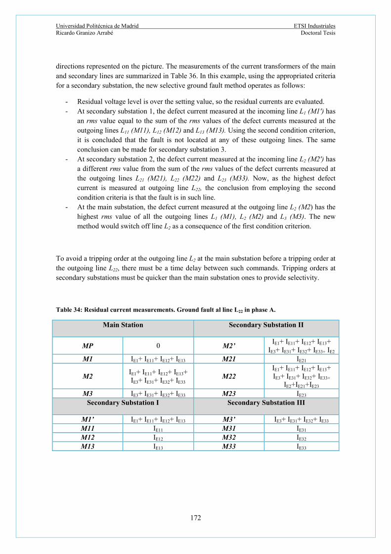
Universidad Politécnica de Madrid ETSI Industriales Ricardo Granizo Arrabé Doctoral Tesis
172
directions represented on the picture. The measurements of the current transformers of the main and secondary lines are summarized in Table 36. In this example, using the appropriated criteria for a secondary substation, the new selective ground fault method operates as follows:
- Residual voltage level is over the setting value, so the residual currents are evaluated. - At secondary substation 1, the defect current measured at the incoming line L1 (M1') has
an rms value equal to the sum of the rms values of the defect currents measured at the outgoing lines L11 (M11), L12 (M12) and L13 (M13). Using the second condition criterion, it is concluded that the fault is not located at any of these outgoing lines. The same conclusion can be made for secondary substation 3.
- At secondary substation 2, the defect current measured at the incoming line L2 (M2') has a different rms value from the sum of the rms values of the defect currents measured at the outgoing lines L21 (M21), L22 (M22) and L23 (M33). Now, as the highest defect current is measured at outgoing line L22, the conclusion from employing the second condition criteria is that the fault is in such line.
- At the main substation, the defect current measured at the outgoing line L2 (M2) has the highest rms value of all the outgoing lines L1 (M1), L2 (M2) and L3 (M3). The new method would switch off line L2 as a consequence of the first condition criterion.
To avoid a tripping order at the outgoing line L2 at the main substation before a tripping order at the outgoing line L22, there must be a time delay between such commands. Tripping orders at secondary substations must be quicker than the main substation ones to provide selectivity.
Table 34: Residual current measurements. Ground fault al line L22 in phase A.
Main Station Secondary Substation II
MP 0 M2’ IE1+ IE11+ IE12+ IE13+
IE3+ IE31+ IE32+ IE33+ IE2 M1 IE1+ IE11+ IE12+ IE13 M21 IE21
M2 IE1+ IE11+ IE12+ IE13+ IE3+ IE31+ IE32+ IE33
M22 IE1+ IE11+ IE12+ IE13+ IE3+ IE31+ IE32+ IE33+
IE2+IE21+IE23 M3 IE3+ IE31+ IE32+ IE33 M23 IE23
Secondary Substation I Secondary Substation III
M1’ IE1+ IE11+ IE12+ IE13 M3’ IE3+ IE31+ IE32+ IE33 M11 IE11 M31 IE31 M12 IE12 M32 IE32 M13 IE13 M33 IE33
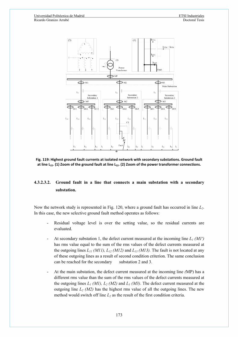
Universidad Politécnica de Madrid ETSI Industriales Ricardo Granizo Arrabé Doctoral Tesis
173
Fig. 119: Highest ground fault currents at isolated network with secondary substations. Ground fault at line L22. (1) Zoom of the ground fault at line L22. (2) Zoom of the power transformer connections.
4.3.2.3.2. Ground fault in a line that connects a main substation with a secondary
substation.
Now the network study is represented in Fig. 120, where a ground fault has occurred in line L2. In this case, the new selective ground fault method operates as follows:
- Residual voltage level is over the setting value, so the residual currents are evaluated.
- At secondary substation 1, the defect current measured at the incoming line L1 (M1') has rms value equal to the sum of the rms values of the defect currents measured at the outgoing lines L11 (M11), L12 (M12) and L13 (M13). The fault is not located at any of these outgoing lines as a result of second condition criterion. The same conclusion can be reached for the secondary substation 2 and 3.
- At the main substation, the defect current measured at the incoming line (MP) has a different rms value than the sum of the rms values of the defect currents measured at the outgoing lines L1 (M1), L2 (M2) and L3 (M3). The defect current measured at the outgoing line L2 (M2) has the highest rms value of all the outgoing lines. The new method would switch off line L2 as the result of the first condition criteria.
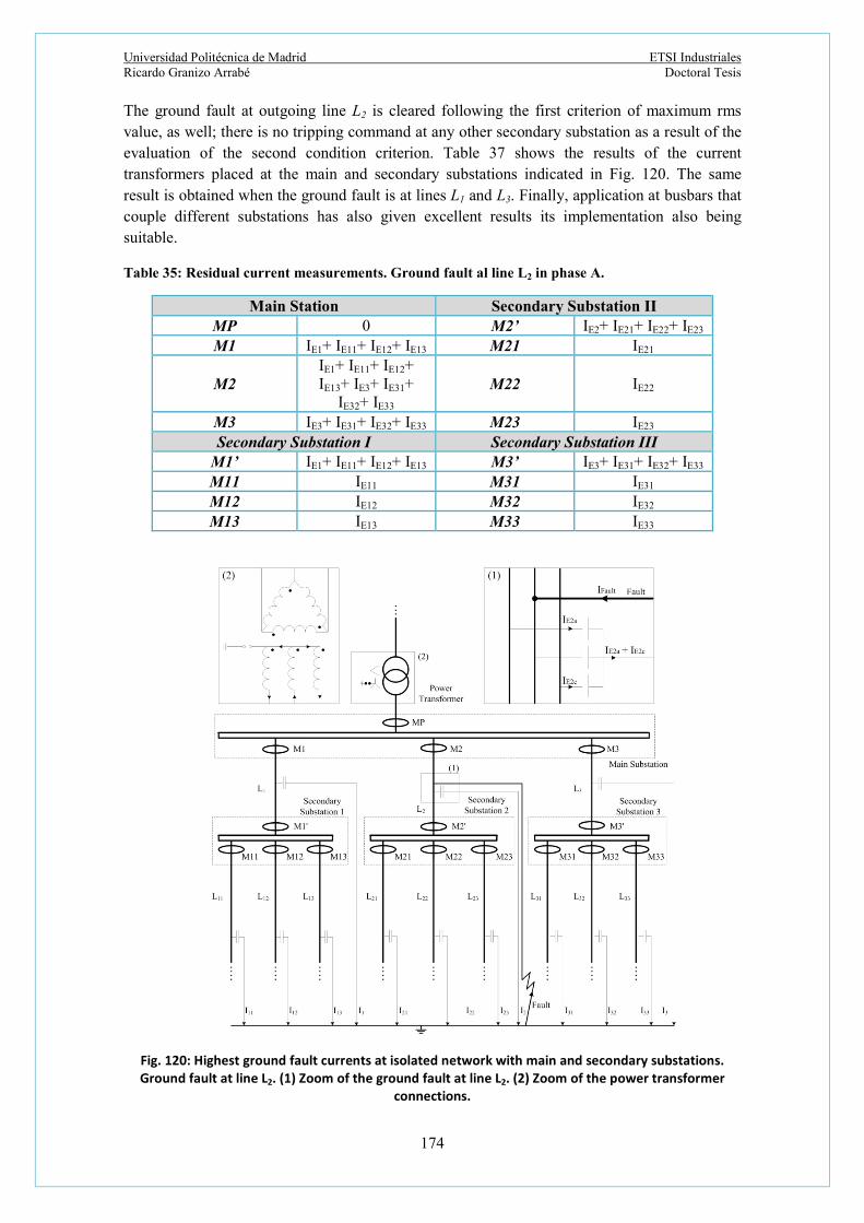
Universidad Politécnica de Madrid ETSI Industriales Ricardo Granizo Arrabé Doctoral Tesis
174
The ground fault at outgoing line L2 is cleared following the first criterion of maximum rms value, as well; there is no tripping command at any other secondary substation as a result of the evaluation of the second condition criterion. Table 37 shows the results of the current transformers placed at the main and secondary substations indicated in Fig. 120. The same result is obtained when the ground fault is at lines L1 and L3. Finally, application at busbars that couple different substations has also given excellent results its implementation also being suitable.
Table 35: Residual current measurements. Ground fault al line L2 in phase A.
Main Station Secondary Substation II MP 0 M2’ IE2+ IE21+ IE22+ IE23 M1 IE1+ IE11+ IE12+ IE13 M21 IE21
M2 IE1+ IE11+ IE12+ IE13+ IE3+ IE31+
IE32+ IE33 M22 IE22
M3 IE3+ IE31+ IE32+ IE33 M23 IE23 Secondary Substation I Secondary Substation III
M1’ IE1+ IE11+ IE12+ IE13 M3’ IE3+ IE31+ IE32+ IE33 M11 IE11 M31 IE31 M12 IE12 M32 IE32 M13 IE13 M33 IE33
Fig. 120: Highest ground fault currents at isolated network with main and secondary substations. Ground fault at line L2. (1) Zoom of the ground fault at line L2. (2) Zoom of the power transformer
connections.

Universidad Politécnica de Madrid ETSI Industriales Ricardo Granizo Arrabé Doctoral Tesis
175
4.3.3. Analysis of simulation results.
The proposed selective ground fault protection method was simulated using ATP (Alternative Transient Program) while post-processing was done using Matlab. An equivalent “pi” model for lines was used as well as power transformers rated 132/20 kV, 10 MVA with YNd11 connection group. The simplest and simplified schematic with one incoming line with 50 km length and three outgoing lines with equal lengths of 150 km without any load connected (a) and the same circuit with different loads (b) are shown in Fig. 121. Three different loads were considered: Z1=960+j719.42 Ω; Z2=545+j263.89 Ω; Z3=380+j124.72 Ω. The parameters of any equivalent “pi” feeder for conductor type LA56 are:
Table 38: Characteristics of LA56 conductor.
Conductor LA56
Diameter: 9.45 mm
Disposition: Delta
Distance conductors a-b: 4 m
Distance conductors b-c: 2.332 m
Distance conductor –c-a: 2.3324 m
Resistance: 0.6136 Ω/km
Inductive reactnce: 0.4148 Ω/km
Capacitance: 0.28 μF/km
4.3.3.1. Main Substation.
To simulate the new method for the detection of which line suffers a ground fault condition, a power system formed by three outgoing lines, of identical lengths, has been used, as seen in Fig. 121. Simulations with load (a) and without load (b) at each line terminal have been carried out. In the simulation, ground faults were simulated at different phases and at different places with different resistance values up to 30 Ω. For instance, a ground fault at single line diagram shown in Fig. 121 is evaluated at line L1 phase ”a” under no load conditions. Voltages under such fault condition at the distribution 20 kV busbars are shown in Fig.122. Voltages at the same distribution 20 kV busbars under the same fault conditions as before but with load in the three feeders turned out to be not so high, between 8 and 10 kV less. In Fig. 123, all ground fault currents of all lines connected to the 20 kV busbars are represented considering the network as indicated in Fig. 121 with load (b). The simulation results shown in Fig. 123 are indicated in Table 3. It can be clearly observed that the line with the defect is the one which has the greatest residual current, being its value the sum of the other residual currents (IE1 = IE2 + IE3 + IE0).

Universidad Politécnica de Madrid ETSI Industriales Ricardo Granizo Arrabé Doctoral Tesis
176
It is totally correct to say that using this proposed method in a main substation; it can easily be detected a ground fault in a selective way.
Fig.121: ATP single line diagram for main substation arrangement.
Fig. 121: Phase voltages at main distribution busbars. Single ground fault at phase “a” in Line L1.
Fig. 122: Phase voltages at main distribution busbars. Single ground fault at phase “a” in Line L1.

Universidad Politécnica de Madrid ETSI Industriales Ricardo Granizo Arrabé Doctoral Tesis
177
Fig. 123: Phase currents at main distribution busbars. Single ground fault at phase “a” in Line L1.
4.3.3.2. Secondary Substations.
Fig. 124 shows a network with one main substation and four secondary substations. Feeders L11, L12, L31, L32, L33, L41 and L42 supply different loads while feeders L2, L34 and L43 are energized without any load connected. Ground fault at line L2 in phase "a" is evaluated and the result shows that ground fault current measurements at 20 kV busbars verify the proposed method. Ground fault currents at outgoing lines L1, L3 and L4 with no fault, keep the same phase angle whereas the ground fault current at the line with ground defect L2 has a 180º phase angle difference compared to those of L1, L3 and L4 in Fig.125. The sum of the rms ground fault current values of lines L0, L1, L3 and L4 is practically the same as that in line L2.
On the other hand, the evaluation of the defect currents at the three secondary substations has shown that the incoming defect current rms value has the same defect current value as has the sum of the rms defect current values of all the outgoing lines, at each of the three secondary substations. Therefore, no tripping command will be given at any other secondary substation. Evaluation of the highest defect current rms value at the main substation will give a tripping order to the line L2 switchgear where the ground fault is taking place. These results are listed in Table 40. In Fig. 125, the ground fault currents of all lines connected to the 20 kV busbars are represented.
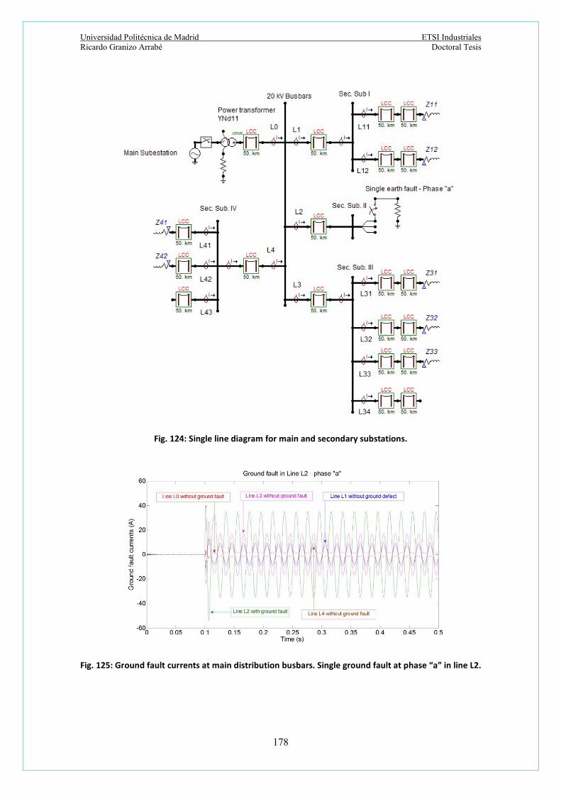
Universidad Politécnica de Madrid ETSI Industriales Ricardo Granizo Arrabé Doctoral Tesis
178
Fig. 124: Single line diagram for main and secondary substations.
Fig. 125: Ground fault currents at main distribution busbars. Single ground fault at phase “a” in line L2.

Universidad Politécnica de Madrid ETSI Industriales Ricardo Granizo Arrabé Doctoral Tesis
179
Table 39: Residual current measurements. Ground fault at line L1 - Phase A.
Main Station IE0 IE1 IE2 IE3
(a) 3.71 25.81 11.05 11.05 (b) 3.10 21.78 9.34 9.34
Table 40: Residual Current Measurements. Ground Fault at Line L2 - Phase A.
Main Station IE0 IE1 IE2 IE3 IE4
1.25 6.44 24.80 11.92 5.19 Secondary Substation I
IE1 IE11 IE12 5.17 2.58 2.59
Secondary Substation II IE2 IE2
24.80 24.80 Secondary Substation III
IE30 IE31 IE32 IE33 IE34 10.63 2.66 2.67 2.67 2.65
Secondary Substation IV IE4 IE41 IE42 IE43
3.92 1.31 1.31 1.31
4.3.4. Experimental results.
To test the validity of the proposed ground fault detection method and its computer simulation results, different laboratory tests have been performed on an isolated network. These tests try to verify the operating principle of the detection technique.
4.3.4.1. Experimental Setup.
The tests were carried out on an isolated network supplied by a power transformer rated 800 VA, 400/100 Vac and YNy0 connection group. Up to nine line modules with equivalent circuit “pi” were used, as shown in Fig. 126. A per unit system of SB = 800 VA, UB = 100 V, IB = 4.618 A and ZB = 12.5 Ω was selected to represent all values. These practical tests were carried out with loads and no loads at the end of the lines. The parameters of any equivalent “pi” feeder, also shown in Fig. 126, have the following characteristics: R=88.48 mΩ, L=4 mH and C=4 μF each capacitor.

Universidad Politécnica de Madrid Ricardo Granizo Arrabé
Fig. 126: Top: Actual network experiment setEquivalent pi line module, 3: Ground fault resistance). Bottom: Equivalent pi
Fig. 127: Single line diagram with three lines with equal length. Single phase fault at phase
180
Top: Actual network experiment set-up. Three identical lines. (1: Power transformer, 2: module, 3: Ground fault resistance). Bottom: Equivalent pi line m
parameter values.
Single line diagram with three lines with equal length. Single phase fault at phase L1.
ETSI Industriales Doctoral Tesis
(1: Power transformer, 2: line module and
Single line diagram with three lines with equal length. Single phase fault at phase “a” in line

Universidad Politécnica de Madrid ETSI Industriales Ricardo Granizo Arrabé Doctoral Tesis
181
Several single ground faults at different phases, lines, and configurations were implemented in the real isolated network erected in the laboratory. The ground fault resistance was shifted from 0 to 2.4 p.u. in all cases studied.
4.3.4.2. Three Lines with Identical Lengths.
This kind of single line network scheme is shown in Fig. 127, where the lines have a total equivalent length of 150 km. Without any load connected (c), the measurements taken when a single ground fault is present at line L1 are listed in Table 41, including the fault resistance Rf and the residual voltage U0 measured at the busbars. The results show that the defect current measured at line L1 has the highest value, compared to those registered at lines L2 and L3. As shown in Table 41, the faults can be clearly located with different fault resistance values, chosen at random. The results obtained when having loads (d) as 300 VA in line L1, 50 VA in line L2 and 150 VA in line L3 are listed in Table 42. Again, the results show that the defect current measured at line L1 has the highest value, compared to those registered at lines L2 and L3.
Table 41: Experimental results. Three lines not loaded with identical length. Residual current measurements IE in per unit values [p.u.]. Ground fault in line L1 – Phase A.
Main Station
Rf U0 L1 L2 L3 IE1,a
0.00 1.38 0.80 0.40 0.40 1.18
0.32 1.21 0.70 0.35 0.35 1.03
0.56 1.19 0.73 0.34 0.34 0.97
0.80 1.03 0.59 0.30 0.30 0.88
1.04 0.82 0.47 0.24 0.24 0.70
1.20 0.75 0.47 0.23 0.23 0.69
1.60 0.62 0.36 0.18 0.18 0.53
2.00 0.53 0.30 0.15 0.15 0.45
2.40 0.47 0.26 0.13 0.13 0.39
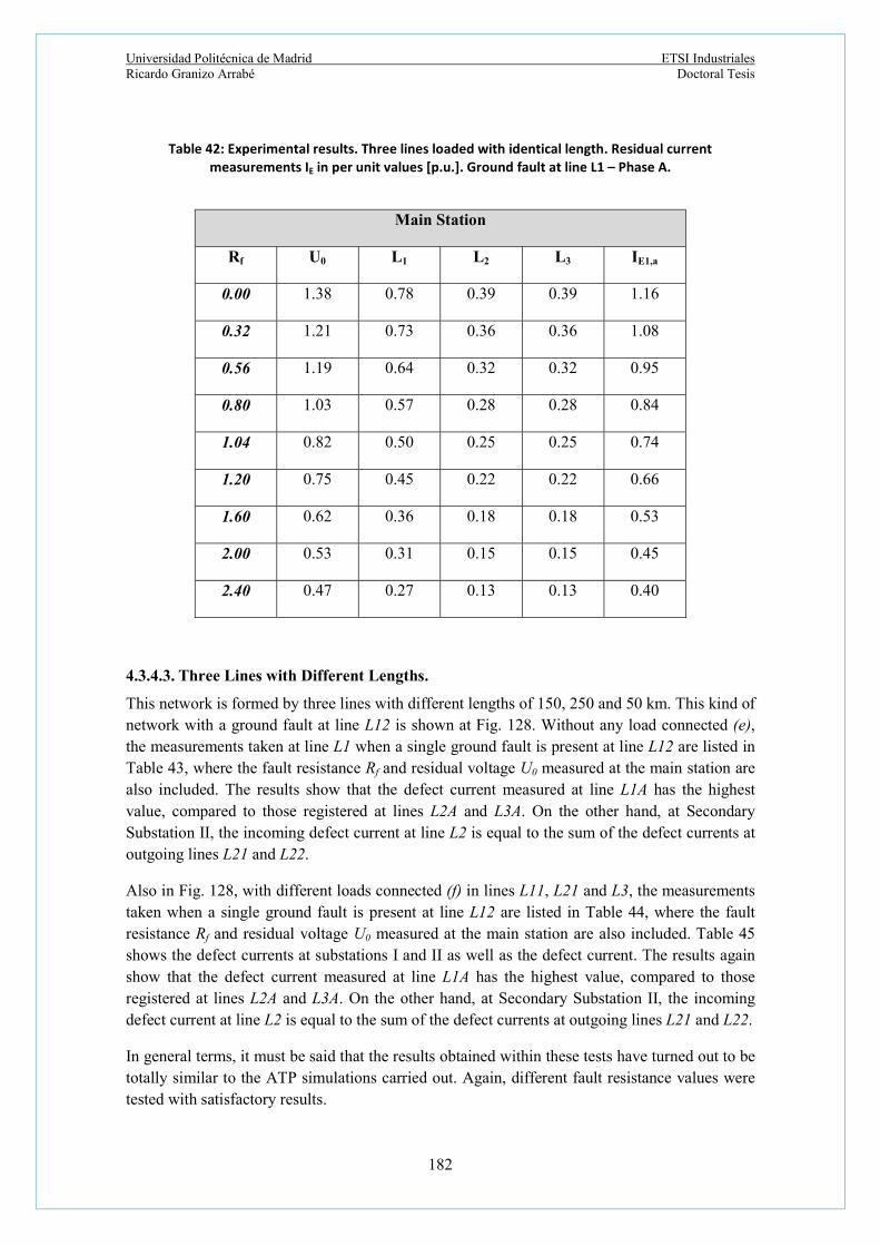
Universidad Politécnica de Madrid ETSI Industriales Ricardo Granizo Arrabé Doctoral Tesis
182
Table 42: Experimental results. Three lines loaded with identical length. Residual current measurements IE in per unit values [p.u.]. Ground fault at line L1 – Phase A.
Main Station
Rf U0 L1 L2 L3 IE1,a
0.00 1.38 0.78 0.39 0.39 1.16
0.32 1.21 0.73 0.36 0.36 1.08
0.56 1.19 0.64 0.32 0.32 0.95
0.80 1.03 0.57 0.28 0.28 0.84
1.04 0.82 0.50 0.25 0.25 0.74
1.20 0.75 0.45 0.22 0.22 0.66
1.60 0.62 0.36 0.18 0.18 0.53
2.00 0.53 0.31 0.15 0.15 0.45
2.40 0.47 0.27 0.13 0.13 0.40
4.3.4.3. Three Lines with Different Lengths.
This network is formed by three lines with different lengths of 150, 250 and 50 km. This kind of network with a ground fault at line L12 is shown at Fig. 128. Without any load connected (e), the measurements taken at line L1 when a single ground fault is present at line L12 are listed in Table 43, where the fault resistance Rf and residual voltage U0 measured at the main station are also included. The results show that the defect current measured at line L1A has the highest value, compared to those registered at lines L2A and L3A. On the other hand, at Secondary Substation II, the incoming defect current at line L2 is equal to the sum of the defect currents at outgoing lines L21 and L22.
Also in Fig. 128, with different loads connected (f) in lines L11, L21 and L3, the measurements taken when a single ground fault is present at line L12 are listed in Table 44, where the fault resistance Rf and residual voltage U0 measured at the main station are also included. Table 45 shows the defect currents at substations I and II as well as the defect current. The results again show that the defect current measured at line L1A has the highest value, compared to those registered at lines L2A and L3A. On the other hand, at Secondary Substation II, the incoming defect current at line L2 is equal to the sum of the defect currents at outgoing lines L21 and L22.
In general terms, it must be said that the results obtained within these tests have turned out to be totally similar to the ATP simulations carried out. Again, different fault resistance values were tested with satisfactory results.

Universidad Politécnica de Madrid ETSI Industriales Ricardo Granizo Arrabé Doctoral Tesis
183
Fig. 128: Multiple line network with ground fault in line L12.
Table 43: Experimental results for three lines not loaded with different lengths. Residual current measurements IE in per unit values [p.u.] with ground fault in line L12 – Phase A.
Main Station Secondary Substation II
Rf U0 L1A L2A L3A IE12,a L2 L21 L22
0.00 0.72 0.73 0.61 0.12 1.08 0.37 0.25 0.12
0.32 0.66 0.71 0.59 0.11 1.04 0.34 0.23 0.11
0.55 0.61 0.68 0.56 0.11 1.00 0.31 0.21 0.10
0.80 0.51 0.58 0.49 0.10 0.87 0.27 0.18 0.09
1.04 0.48 0.49 0.38 0.07 0.68 0.25 0.17 0.08
1.20 0.40 0.45 0.37 0.07 0.66 0.21 0.14 0.07
1.60 0.33 0.36 0.30 0.06 0.53 0.17 0.12 0.05
2.00 0.28 0.30 0.25 0.05 0.44 0.14 0.10 0.04
2.40 0.24 0.27 0.23 0.02 0.39 0.12 0.08 0.04
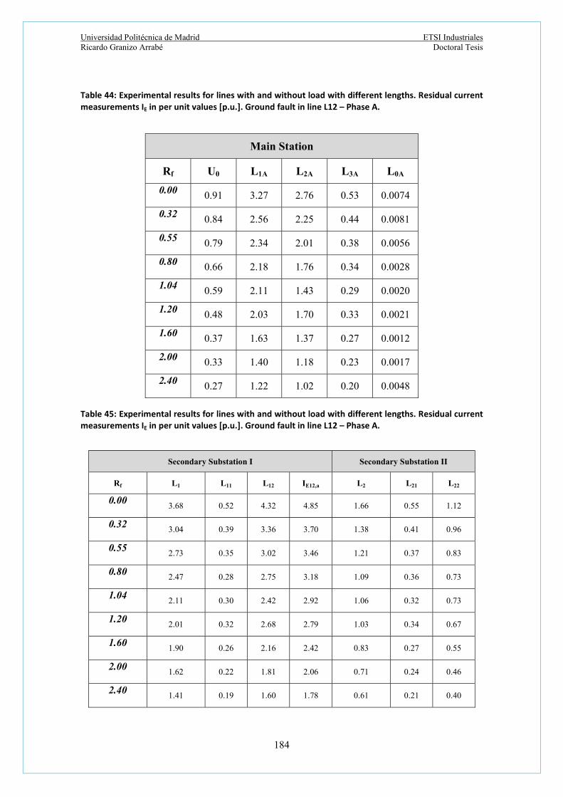
Universidad Politécnica de Madrid ETSI Industriales Ricardo Granizo Arrabé Doctoral Tesis
184
Table 44: Experimental results for lines with and without load with different lengths. Residual current measurements IE in per unit values [p.u.]. Ground fault in line L12 – Phase A.
Main Station
Rf U0 L1A L2A L3A L0A
0.00 0.91 3.27 2.76 0.53 0.0074
0.32 0.84 2.56 2.25 0.44 0.0081
0.55 0.79 2.34 2.01 0.38 0.0056
0.80 0.66 2.18 1.76 0.34 0.0028
1.04 0.59 2.11 1.43 0.29 0.0020
1.20 0.48 2.03 1.70 0.33 0.0021
1.60 0.37 1.63 1.37 0.27 0.0012
2.00 0.33 1.40 1.18 0.23 0.0017
2.40 0.27 1.22 1.02 0.20 0.0048
Table 45: Experimental results for lines with and without load with different lengths. Residual current measurements IE in per unit values [p.u.]. Ground fault in line L12 – Phase A.
Secondary Substation I Secondary Substation II
Rf L1 L11 L12 IE12,a L2 L21 L22
0.00 3.68 0.52 4.32 4.85 1.66 0.55 1.12
0.32 3.04 0.39 3.36 3.70 1.38 0.41 0.96
0.55 2.73 0.35 3.02 3.46 1.21 0.37 0.83
0.80 2.47 0.28 2.75 3.18 1.09 0.36 0.73
1.04 2.11 0.30 2.42 2.92 1.06 0.32 0.73
1.20 2.01 0.32 2.68 2.79 1.03 0.34 0.67
1.60 1.90 0.26 2.16 2.42 0.83 0.27 0.55
2.00 1.62 0.22 1.81 2.06 0.71 0.24 0.46
2.40 1.41 0.19 1.60 1.78 0.61 0.21 0.40

Universidad Politécnica de Madrid ETSI Industriales Ricardo Granizo Arrabé Doctoral Tesis
185
4.3.4.4. Conclusions.
This new selective ground fault technique for ungrounded networks has been researches, simulated and tested. This new method is suitable for all kinds of main substations with at least three feeders and secondary substations. The proposed non directional detection technique is based on the comparison of the value of the ground fault currents at each line position of each substation. At main substations, the highest ground fault current module belongs to the line with the ground fault. At secondary substations, if the ground fault current at the incoming line of the main busbars has the same value as the arithmetic sum of all outgoing ground fault currents, the fault is not located at any of the outgoing lines connected to those busbars, provided that a minimum residual voltage over an established setting value is present. ATP simulations with different substation configurations turned out to be totally satisfactory as well as the experimental results of the laboratory tests. All of them show that the localization of the ground fault is easy to find, without any possible mistake, identifying the corresponding line as the “line with ground fault condition". This new protection technique has the following advantages, when compared to traditional directional ground fault protection devices:
1. It is much easier to measure the values of the ground defect currents than evaluate the direction of the ground defect currents compared to the residual voltage.
2. In substations that can´t be removed from service, primary injection tests aren´t able to be developed and the correct operation of the directional ground fault protection relays is not secured whereas this new method is able to be totally commissioned without primary injection tests and its good performance can be granted without removing the substation from service.
3. Unintentional wrong tripping commands given by directional protection relays due to wrong CT´s and VT´s polarities connections are avoided as directional criterion are not used.
4. It reduces dramatically the time and costs of installation and commissioning compared to the use of directional ground fault protection relays. The costs of three voltage transformers in medium voltage systems are estimated in 1.500 EUR/unit, 1.200 EUR/unit for a directional ground fault protection relay and about 200 EUR/unit for the ring core currents transformer or 1.300 EUR/unit for outdoor current transformers. The new method only needs the current transformers and the protection relay which cost is estimated in 3.500 EUR/unit.
The aforementioned advantages provide a great improvement in the network protection system as unintended trips caused by single ground faults are eliminated.
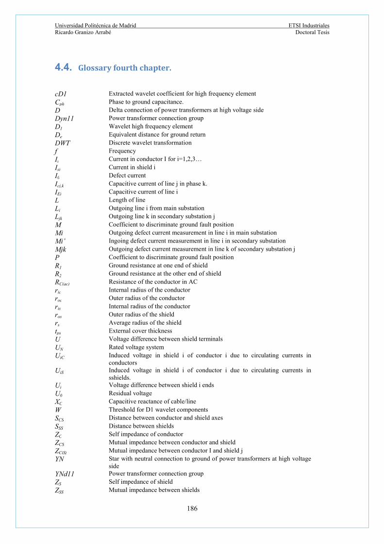
Universidad Politécnica de Madrid ETSI Industriales Ricardo Granizo Arrabé Doctoral Tesis
186
4.4. Glossary fourth chapter.
cD1 Extracted wavelet coefficient for high frequency element Cph Phase to ground capacitance. D Delta connection of power transformers at high voltage side Dyn11 Power transformer connection group D1 Wavelet high frequency element De Equivalent distance for ground return DWT Discrete wavelet transformation f Frequency Ii Current in conductor I for i=1,2,3… Isi Current in shield i I0 Defect current Icj,k Capacitive current of line j in phase k. IEi Capacitive current of line i L Length of line Li Outgoing line i from main substation Ljk Outgoing line k in secondary substation j M Coefficient to discriminate ground fault position Mi Outgoing defect current measurement in line i in main substation Mi’ Ingoing defect current measurement in line i in secondary substation Mjk Outgoing defect current measurement in line k of secondary substation j P Coefficient to discriminate ground fault position R1 Ground resistance at one end of shield R2 Ground resistance at the other end of shield RC(ac) Resistance of the conductor in AC ric Internal radius of the conductor roc Outer radius of the conductor ris Internal radius of the conductor ros Outer radius of the shield rs Average radius of the shield tps External cover thickness
U Voltage difference between shield terminals UN Rated voltage system UiC Induced voltage in shield i of conductor i due to circulating currents in
conductors UiS Induced voltage in shield i of conductor i due to circulating currents in
sshields. Ui Voltage difference between shield i ends U0 Residual voltage XC Capacitive reactance of cable/line W Threshold for D1 wavelet components SCS Distance between conductor and shield axes SSS Distance between shields ZC Self impedance of conductor ZCS Mutual impedance between conductor and shield ZCiSj Mutual impedance between conductor I and shield j YN Star with neutral connection to ground of power transformers at high voltage
side YNd11 Power transformer connection group ZS Self impedance of shield ZSS Mutual impedance between shields
Universidad Politécnica de Madrid ETSI Industriales Ricardo Granizo Arrabé Doctoral Tesis
187
ZSiSj Mutual impedance between shields i-j ΔLiSi Angle difference between conductor i and shield i ρe Ground resistivity μ0 Vacuum permeability

Universidad Politécnica de Madrid ETSI Industriales Ricardo Granizo Arrabé Doctoral Tesis
188

Universidad Politécnica de Madrid ETSI Industriales Ricardo Granizo Arrabé Doctoral Tesis
189
5. NEW PROTECTION METHODS FOR DC
POWER SYSTEMS.

Universidad Politécnica de Madrid ETSI Industriales Ricardo Granizo Arrabé Doctoral Tesis
190
his chapter describes the High Voltage Direct Current (HVDC) systems normally used in transmission systems that use insulated power cables. Again, the circulation of currents in the shields of the power cables is studied, simulated and tested in laboratory
with the aim of finding out new trends to find out new detection methods to locate the ground faults in a selective way.
5.
T

Universidad Politécnica de Madrid ETSI Industriales Ricardo Granizo Arrabé Doctoral Tesis
191
5.1. Introduction.
The use of electrical direct current power systems in transmision and distribution is having relevant importance worldwide as there are many new HVDCs systems set in operation year after year: three in Africa, five in Oceania, fifty five in Asia, sixty five in Europe, twenty one in North America and four in South America [141]. As result of the amount of HVDCs systems planned to be erected worldwide, new protection methods for ground fault detection have been developed within this research works.
The results concude with three new methods for ground fault detection in HVDCs power cable systems:
- Diferential ground fault detection method. - Directional ground fault detection method. - Method for discrimination between switching-on and ground fault currents.
5.2. MATLAB-SIMULINK model implemented for new protection methods for HVDC power cable systems.
The model used in Matlab-Simulink is illustrated in Fig. 129. Three different sections of cable rated 220 kV and lengths of 100 km each one are considered.

Universidad Politécnica de Madrid ETSI Industriales Ricardo Granizo Arrabé Doctoral Tesis
192
Fig. 129: Model for new methods of ground fault and energizing currents.
Continuous
powergui
v+-
Ucarga
Con
n1
Subsystem
Series RLC Branch2Series RLC Branch1
Scope6
Scope5
Scope4
Scope3
Scope2
Scope10
Scope1
i+
-
Retorno1
R9
R25R24
R10
R1
i+
-
Icarga
i+-
I2
i+-
I1
2
I(R1)5
1
I(R1)4
1
I(R1)3
1
I(R1)2
1
I(R1)1
1
I(R1)
Co
nn2
Co
nn1
Generación2
Carga50 MW
Cable 1
screen 1
Cable 1
screen 1
Cable + Pantalla2
Cable 1
screen 1
Cable 1
screen 1
Cable + Pantalla1
Cable 1
screen 1
Cable 1
screen 1
Cable + Pantalla
Breaker2
Breaker1
Breaker

Universidad Politécnica de Madrid Ricardo Granizo Arrabé
193
The technical characteristics of the cable used in the model are:
Table 46 Main characteristics of 220 kV cable.
Library: Simscape
Category: SimPowerSystems
Element: Mutual Inductance + Series RLC Branch
Parameters:
R= detailed matrix. L= detailed matrix. C= detailed matrix. ρAl =2,82.10-8 Ω.m ρCu =1,71.10-8 Ω.m
ρe =100 Ω.m εcs=2,5 εse=2,3 r=3%
f=50 Hz
Length= 100 km trams
Table 47: Dimensional characteristics of 220 kV cable.
Nominal voltage
(kV)
Cross section
Cu (mm2)
Shield cross
section
Cu (mm2)
Outer diameter
(mm)
Maximum insulation
temperature (ºC)
Maximum cover
temperature
(ºC)
220 2000 165 130 90 70
A cross section is shown in Fig. 130.

Universidad Politécnica de Madrid ETSI Industriales Ricardo Granizo Arrabé Doctoral Tesis
194
Fig. 130: Physical dimensions of the cable used in the model.
The equivalent PI circuit of this cable considers the mutual impedance between the conductor and the shield as well as the capacitances conductor-shield and shield-ground.
Fig. 131: PI model of the cable used.
The model circuit used is shown in Fig. 132. It consists in three cable stretches, two HVDC generation systems, one load placed at HVDC generation system G2 and a fault circuit breaker that allows us to place the ground fault at any position along the cables.
Simulations have shown the next values for the currents circulating in the shields for ground faults that take place at different positions. The power system simulated has different loads.
The simulation model considers a system rated 220 kVdc and loads from 0 to 50 MW connected.

Universidad Politécnica de Madrid ETSI Industriales Ricardo Granizo Arrabé Doctoral Tesis
195
Fig. 132: Model for analysis switching-on currents in shields of a cable 220 kVdc without load connected.

Universidad Politécnica de Madrid Ricardo Granizo Arrabé
196
5.3. Differential ground fault detection method for DC insulated cables.
This research presents a novel method for selective detection of ground faults in DC cables that have their shields grounded at both ends [142]. It is so the cable that has a ground fault is identified by measuring the currents of the defect at the ends of the two cable shields. These two currents have opposite polarity if the cable is not faulty. On the other hand, if the cable is defective, the two currents have equal polarities. It also knows and identifies the cable with ground fault by measuring and comparing the currents that circulate at the two ends of the shield. Therefore the discrimination between the currents corresponding to switching maneuvers of connection of protected cables and the corresponding currents with ground faults is achieved. This way, erroneous or improper tripping commands are eliminated.
5.3.1. Background of the method.
This method presents a new method and for differential detection of ground faults in DC power networks with insulated cables. This method offers a perfect detection of the defective insulated cable, ensuring total selectivity to avoid unwanted or erroneous tripping commands. It does not use any DC busbar voltage value that could be measured in the network protected by this method.
When a ground fault occurs in DC networks, the value of said defect intensity can have very high values. Fast detection and clearing are a must since all power elements that make up the DC grid are subjected to high thermal stresses, being able to deteriorate their insulation and cause severe damage. In some applications, a system is used to detect the fault not yet being selective has good results. This system injects a voltage signal of small amplitude. This way the value of the insulation resistance in each cable is calculated continuously. Once the value of the level of isolation descends to values corresponding to situations considered defective, the system first provides an alarm signal and, in case of progressive descent of the insulation, a second tripping signal is released. This technique has been used normally in low voltage electrical distribution networks.
Some patents describe possible solutions to this technical problem, such as:
- EN 2 231 270 B2 ("System and method for detecting ground faults in DC systems fed by rectifiers "). Although the systema and method described in this patent detect defects to earth in DC networks, mainly in the excitation systems of synchronous generators, their application is not suitable for the protection of long DC cables.
- WO2011157305 ("FAULT PROTECTION OF HVDC TRANSMISSION LINES"). This patent detects and clears defects in DC cables reading the values of voltage and intensity that appear in coils arranged in series with the DC cable itself and the
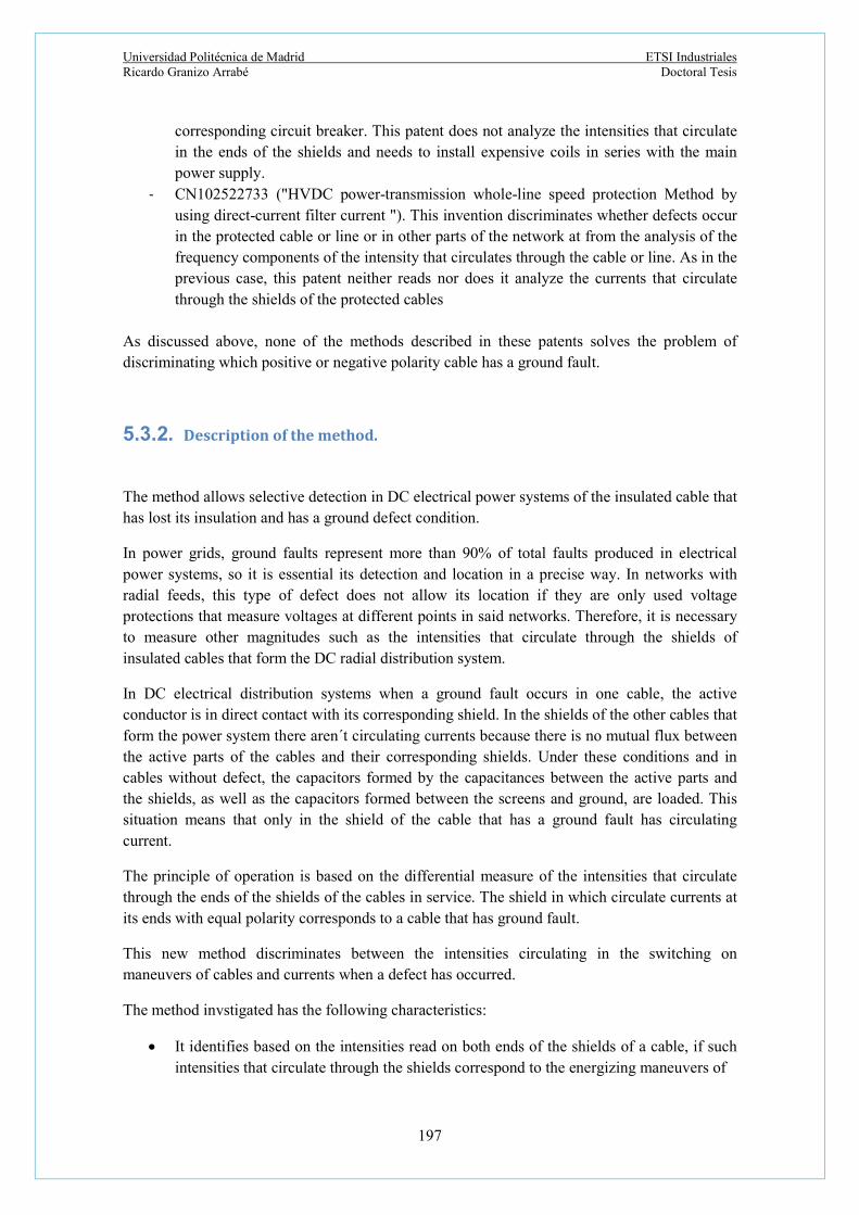
Universidad Politécnica de Madrid ETSI Industriales Ricardo Granizo Arrabé Doctoral Tesis
197
corresponding circuit breaker. This patent does not analyze the intensities that circulate in the ends of the shields and needs to install expensive coils in series with the main power supply.
- CN102522733 ("HVDC power-transmission whole-line speed protection Method by using direct-current filter current "). This invention discriminates whether defects occur in the protected cable or line or in other parts of the network at from the analysis of the frequency components of the intensity that circulates through the cable or line. As in the previous case, this patent neither reads nor does it analyze the currents that circulate through the shields of the protected cables
As discussed above, none of the methods described in these patents solves the problem of discriminating which positive or negative polarity cable has a ground fault.
5.3.2. Description of the method.
The method allows selective detection in DC electrical power systems of the insulated cable that has lost its insulation and has a ground defect condition.
In power grids, ground faults represent more than 90% of total faults produced in electrical power systems, so it is essential its detection and location in a precise way. In networks with radial feeds, this type of defect does not allow its location if they are only used voltage protections that measure voltages at different points in said networks. Therefore, it is necessary to measure other magnitudes such as the intensities that circulate through the shields of insulated cables that form the DC radial distribution system.
In DC electrical distribution systems when a ground fault occurs in one cable, the active conductor is in direct contact with its corresponding shield. In the shields of the other cables that form the power system there aren´t circulating currents because there is no mutual flux between the active parts of the cables and their corresponding shields. Under these conditions and in cables without defect, the capacitors formed by the capacitances between the active parts and the shields, as well as the capacitors formed between the screens and ground, are loaded. This situation means that only in the shield of the cable that has a ground fault has circulating current.
The principle of operation is based on the differential measure of the intensities that circulate through the ends of the shields of the cables in service. The shield in which circulate currents at its ends with equal polarity corresponds to a cable that has ground fault.
This new method discriminates between the intensities circulating in the switching on maneuvers of cables and currents when a defect has occurred.
The method invstigated has the following characteristics:
It identifies based on the intensities read on both ends of the shields of a cable, if such intensities that circulate through the shields correspond to the energizing maneuvers of

Universidad Politécnica de Madrid ETSI Industriales Ricardo Granizo Arrabé Doctoral Tesis
198
the cables. For this, the polarities of the intensities that circulate at both ends of the shield of the protected cable are evaluated and don´t indicate any defect if:
1. The polarities of said intensities are of different sign until the attenuation of
both intensities to values due to the ripple of the system.
2. The polarity of the currents at the ends of the shield change sign at least once until they dim.
It identifies on the basis of the intensities read in the shields of the cables, if such
intensities correspond to ground faults in the DC cables. To do this, it identifies the polarities of the intensities that circulate at both ends of the shield of the protected cable and gives indication when the polarities of said currents have equal sign.
5.3.3. Simulations results: Differential ground fault detection method.
When this kind of fault happens, the trends of currents that circulate in the shield at both ends appear in next figure.
Fig. 133: Current waveforms for ground fault currents in the shield of a faulty conductor without load connected.
It can be observed how different the currents in the shields are from a switching on command to a ground fault. Ground fault current values reach now 8.814 A and 5.904 A.
0 0.5 1 1.5 2 2.5 3-2000
0
2000
4000
6000
8000
10000
Time (s)
Cu
rren
t a
t th
e e
nd
s o
f sh
ield
(A
)
Ground fault at 200 km inside a cable - Currents in shields.
Current in shield - End far away to the fault.Current in shield - End closer to the fault.

Universidad Politécnica de Madrid ETSI Industriales Ricardo Granizo Arrabé Doctoral Tesis
199
Fig. 134: Current waveforms for ground fault currents in the shield of a non-faulty conductor without load connected.
For the same ground fault, Fig. 134 shows the current circulating in the shield of a stretch without defect. At both ends such current has the same value about 5.815 A, and different polarity. Tables 48, 49 and 50 show the polarity of currents circulating at both ends of the shield in every stretch for different ground faults along the conductor. It has also been considered three stretches with 100 km each one. At every end of any shield, currents leaving the shield have been considered as positive and currents entering in the shield negative.
Table 48: Polarities of ground fault shield currents in stretch 1 with 50 MW load connected.
Ground fault in stretch 1
Polarity in currents at ends of the shield
Ground fault
position in
stretch
(km)
Stretch 1 Stretch 2 Stretch 3
End A End B End A End B End A End B
0 positive positive negative positive negative positive
25 positive positive negative positive negative positive
50 positive positive negative positive negative positive
75 positive positive negative positive negative positive
100 positive positive negative positive negative positive
0 0.5 1 1.5 2 2.5 3-6000
-4000
-2000
0
2000
4000
6000
Time (s)
Cu
rre
nt in
sh
ield
s (A
).Current at both ends of a shield in a cable strecht without defect.
Current in shield - left sideCurrent in shield - right side

Universidad Politécnica de Madrid ETSI Industriales Ricardo Granizo Arrabé Doctoral Tesis
200
Table 49: Polarities of ground fault currents in stretch 2 with 50 MW load connected.
Ground fault in stretch 2
Polarity in currents at ends of the shield
Ground fault
position in
stretch
(km)
Stretch 1 Stretch 2 Stretch 3
End A End B End A End B End A End B
0 negative positive positive positive negative positive
25 negative positive positive positive negative positive
50 negative positive positive positive negative positive
75 negative positive positive positive negative positive
100 negative positive positive positive negative positive
Table 50: Polarities of ground fault currents in stretch 3 with 50 MW load connected.
Ground fault in stretch 3
Polarity in currents at ends of the shield
Ground fault
position in
stretch
(km)
Stretch 1 Stretch 2 Stretch 3
End A End B End A End B End A End B
0 negative positive negative positive positive positive
25 negative positive negative positive positive positive
50 negative positive negative positive positive positive
75 negative positive negative positive positive positive
100 negative positive negative positive positive positive
Now, simulations without any load have been developed and their results are listed below.

Universidad Politécnica de Madrid ETSI Industriales Ricardo Granizo Arrabé Doctoral Tesis
201
Table 51: Polarities of ground fault currents in stretch 1 without load connected.
Ground fault in stretch 1
Polarity in currents at ends of the shield
Ground fault
position in
stretch
(km)
Stretch 1 Stretch 2 Stretch 3
End A End B End A End B End A End B
0 positive positive negative positive negative positive
25 positive positive negative positive negative positive
50 positive positive negative positive negative positive
75 positive positive negative positive negative positive
100 positive positive negative positive negative positive
Table 52: Polarities of ground fault currents in stretch 2 without load connected.
Ground fault in stretch 2
Polarity in currents at ends of the shield
Ground fault
position in
stretch
(km)
Stretch 1 Stretch 2 Stretch 3
End A End B End A End B End A End B
0 negative positive positive positive negative positive
25 negative positive positive positive negative positive
50 negative positive positive positive negative positive
75 negative positive positive positive negative positive
100 negative positive positive positive negative positive

Universidad Politécnica de Madrid ETSI Industriales Ricardo Granizo Arrabé Doctoral Tesis
202
Table 53: Polarities of ground fault currents in stretch 3 without load connected.
Ground fault in stretch 3
Polarity in currents at ends of the shield
Ground fault
position in
stretch
(km)
Stretch 1 Stretch 2 Stretch 3
End A End B End A End B End A End B
0 negative positive negative positive positive positive
25 negative positive negative positive positive positive
50 negative positive negative positive positive positive
75 negative positive negative positive positive positive
100 negative positive negative positive positive positive
It has been observed how the results are identical. Polarities of currents in the shields are the same when there is any load connected or not. These results give good evidence of the discrimination of the stretch where the ground fault took place.
5.3.4. Experimental model implemented in laboratory.
The test circuit implemented in the laboratory is formed by:
- Three cable sections with 100 m length each one. Such cables are the same ones used
for the AC test and are described in Section 3.1.3.3.
- One resistor load with range 0-150 Ω.
- One DC rectifying bridge.
- One AC power supply unit.
- One circuit breaker to develop ground faults.
- Clamps FLUKE I30S for measuring currents in the conductor and in its two shield ends.
- An oscilloscope Tektronix TPS2024 with a memory card to save test currents.

Universidad Politécnica de Madrid ETSI Industriales Ricardo Granizo Arrabé Doctoral Tesis
203
Such test configuration appears in Fig. 135:
Fig. 135: Experimental set-up. (1: DC power supply unit; 2: AC power supply; 3: Oscilloscope; 4: Rectifying bridge; 5: Current measurement units; 6: Fault switch; 7: Cables; 8: Current measurement
unit; 9: resistor load; 10: Conductors and shields arrangements.
The lay-out of the ground fault postions in indicated in Fig. 136.
Fig. 136: Lay-out of experimental ground faults positions in A, B, C and D. Switching on commands and different ground faults were carried out along the three sections of the cable with and without resistive load connected. Tests were developed from 40 to 100 Vdc.

Universidad Politécnica de Madrid ETSI Industriales Ricardo Granizo Arrabé Doctoral Tesis
204
5.3.5. Experimental results: Ground fault.
Different ground fault tests at positions A, B, C and D in the layout shown in previous Fig. 136 were performed with resistive loads from 0 to 150 Ω. Fig. 137 shows the ground fault currents for a defect in position B from positive conductor to the corresponding shield with a 1 A load current.
Fig. 137: Ground fault currents with 150 Ω load connected.
It can be observed how the currents circulating at both shield ends of the positive conductor have the same polarity, which represents a clear indication that the cable has a defect. Next figure gives a visual indication of the fault current circulation when a fault happens in stretch 1 and outside the cable.
Fig. 138: Current circulation for a ground fault in stretch 1 and outside the cable.
-0.005 0 0.005 0.01 0.015 0.02 0.025 0.03-0.5
0
0.5
1
1.5
2
2.5
3
3.5
Time (s)
Cu
rre
nts
(A
)
Ground fault currents with load connected
CH1: Current in conductorCH3: Current in shield - Load sideCH4: Current in shield - DC Power Supply Side

Universidad Politécnica de Madrid ETSI Industriales Ricardo Granizo Arrabé Doctoral Tesis
205
Fault currents registered with defects produced at points a, b, c and d are listed in Tables 54 and 55.
Table 54: Ground fault currents in shields with load connected.
Position of the fault
Cable end close to power supply
(A)
Cable length
(m)
Cable end away to power supply
(A)
a 1.416 300 0.511
b 1.408 300 0.508
c 0.584 300 0.372
d 0.328 300 0.304
An example of current trends is included in next figure and tests results without any load connected from the beginning are listed following:
Fig. 139: Ground fault currents without any load connected.
0.07 0.072 0.074 0.076 0.078 0.08 0.082 0.084 0.086 0.088 0.09-0.5
0
0.5
1
1.5
Time (s)
Cu
ren
ts (
A)
Ground fault without load connected
CH1: Current in conductorCH3: Current in shield - end close to the DC Power supplyCH4: Current in shield - end away from the DC Power Supply

Universidad Politécnica de Madrid ETSI Industriales Ricardo Granizo Arrabé Doctoral Tesis
206
Table 55: Ground fault currents in shields without load connected.
Position of the fault
Cable end close to power supply
(A)
Cable length
(m)
Cable end away to power supply
(A)
a 0.372 300 1.032
b 0.360 300 0.363
c 0.360 300 0.363
d 0.330 300 1.041
5.4. Directional ground fault detection method for DC insulated cables.
This research presents a novel directional method for selective detection of ground faults in DC cables that have their shields grounded at both ends. It is so the cable that has a ground fault is identified by measuring the polarity of the currents at the ends of the cable shield and comparing such polarities to the polarity of the corresponding active pole positive or negative. If those polarities are identical, such cable is faulty. On the other hand, if the cable is not defective, the polarities are not all equal. Therefore the discrimination between the currents corresponding to fault and non fault situations is achieved. This way, wrong tripping commands are eliminated.
5.4.1. Background of the method.
This method presents a new method and for directional detection of ground faults in DC power networks with insulated cables. This method also offers a perfect detection of the defective insulated cable, ensuring total selectivity to avoid wrong tripping commands. It uses the DC busbar voltage polarity value that could be measured in the network protected by this method.
When a ground fault occurs in DC networks, the value of said defect intensity normally has very high values. Fast detection and clearing are always a must to avoid damage in the power elemsnt as well as to reduce instability of the DC power system.
Some patents describe possible solutions to this technical problem, such as:
- WO2011157305 ("FAULT PROTECTION OF HVDC TRANSMISSION LINES"). This patent detects and clears defects in DC cables reading the values of voltage and intensity that appear in coils arranged in series with the DC cable itself and the

Universidad Politécnica de Madrid ETSI Industriales Ricardo Granizo Arrabé Doctoral Tesis
207
corresponding circuit breaker. This patent does not analyze the intensities that circulate in the ends of the shields and needs to install expensive coils in series with the main power supply.
- CN102522733 ("HVDC power-transmission whole-line speed protection Method by using direct-current filter current "). This invention discriminates whether defects occur in the protected cable or line or in other parts of the network at from the analysis of the frequency components of the intensity that circulates through the cable or line. As in the previous case, this patent neither reads nor does it analyze the currents that circulate through the shields of the protected cables.
As discussed above, none of the methods described in these patents solves the problem of discriminating which positive or negative polarity cable has a ground fault.
5.4.2. Description of the method.
This method serves to solve the problem mentioned above, solving the drawbacks of the solutions discussed in the state of the art, by measuring the current intensities that circulate through the screens arranged at the ends of the isolated cables that make up any DC distribution network, to compare them with a previously defined threshold and analyzing its polarity to allow or not the shot. The present invention allows to selectively detecting in DC power supply systems, the isolated cable or cables that are in ground fault condition, offering a perfect detection of the isolated cable with defect, besides guaranteeing the indication of the defective cable providing total selectivity to avoid unwanted or erroneous trippings. The operating principle of the present invention is based on the measurement and analysis of the current intensities that circulate through the screens of the cables in service connected to the same supply bars. The screen (s) by which the current is being circulated with the same polarity as the supply voltage of said cables during times exceeding previously established thresholds corresponds to the cables with defect . On the other hand, the screens of the cables through which they circulate intensities with different polarity always or with alternating polarity with respect to the polarity of the supply voltage of said cables, during times higher than previously established thresholds, correspond to the cables without defect. The present invention thus realizes discrimination between the intensities that circulate through the screens in the maneuvers of connection of the cables and the intensities that circulate through the screens when a defect has occurred. In the case of connection maneuvers, the intensities that circulate through the screens of the cables present the following characteristics:
1.- They take positive and negative values until their complete attenuation.
2.- There appear, therefore, oscillations of sign in its derivative with respect to the time until its complete attenuation.

Universidad Politécnica de Madrid ETSI Industriales Ricardo Granizo Arrabé Doctoral Tesis
208
In the case of a defect in the cable, the measured currents present the following characteristics:
1.- The values of the intensity are always positive or negative, they do not change sign.
2.- Oscillations may appear in the sign of its derivative with respect to time.
3.- The values of the intensity have the same polarity as the supply voltage of the cable.
One aspect of the invention relates to a method for detecting faults or ground faults in DC systems of isolated cables, where the grounding of the insulated cables is carried out by means of screens arranged at both ends of the cable to be protected from such defects. , which comprises the following stages:
- Reading / measuring the intensities circulating through the screens to obtain a signal measuring the intensity that flows through the screen of the protected cable, identifying an intensity value and a current polarity value in the intensity measurement signal.
- Comparing the intensity value of the intensity measurement signal with a previously determined reference threshold and comparing the intensity polarity value read with a polarity sign defined for the detection of defects.
- Indicate that there is a defect in the cable based on the previous comparison.
In a possible embodiment, if the intensities read on the screens are higher than the reference threshold, the method proceeds to evaluate the polarities of said intensities with respect to the polarity of the protected cable to obtain a signal indicating failure or defect. If the polarities of the currents flowing through the screens are the same and match the polarity of the protected cable, it is indicated that the cable has a ground fault. And if the polarities of the currents that circulate through the screens of the protected cable are different, said cable has no ground fault.
This method can be summarized as follows:
a. The ground fault detection includes:
- The measuring of the current that circulates through the cable screen. This measurement has a modulus value as well as a polarity.
- The comparisons of the current measured to a threshold previously determined and the current polarity value to the polarity of the voltage supply of the cable.
- The indication that there is a defect in the cable if the current value of the current measurement signal exceeds the previously determined threshold during a time interval that was previously set, and the current polarity value is equal to the supply voltage polarity of the cable.

Universidad Politécnica de Madrid ETSI Industriales Ricardo Granizo Arrabé Doctoral Tesis
209
5.4.3. Simulations results: Directional ground fault detection method.
The simulation circuit used to give evidence of this directional ground fault detection method is the same as employed for the differential ground fault detection method. When this kind of fault happens, the trends of voltages and currents that circulate in the shield at both ends appear in next figures where a fault has been simulated at the positive cable in a DC power system. In Fig. 140 can be seen that after the first 3-5 ms of the fault inception, the polarities of the voltage as well as the currents circulating at the ends of the cable shield have are equal in the stretch with fault. However, in Fig. 141 the polarities of them are not identical in a stretch where the defect is not placed.
Fig. 140: Ground fault at positive pole: DC voltage supply and currents at shield ends in stretch with fault. Currents affected by a scale factor x10.
Fig. 141: Ground fault at positive pole: DC voltage supply and currents at shield ends in stretch without fault. Currents affected by a scale factor x10.
0.98 0.99 1 1.01 1.02 1.03 1.04
-1
-0.5
0
0.5
1
1.5
2
x 105
Time (s)
DC
vo
ltage
/ F
au
lt cu
rre
nts
at t
he
en
ds
of
the
sh
ield
DC Voltage sourceShield current x 10 - End A Shield current x 10 - End B
1 1.005 1.01 1.015 1.02 1.025 1.03 1.035 1.04
-2
-1.5
-1
-0.5
0
0.5
1
1.5
2
x 105
Time (s)
DC
Vo
ltag
e/ C
urr
ent
s in
sh
ield
sof
str
etc
h w
itho
ut
defe
ct
DC Voltage supplyShield current x10 - End AShield current x10 - End B
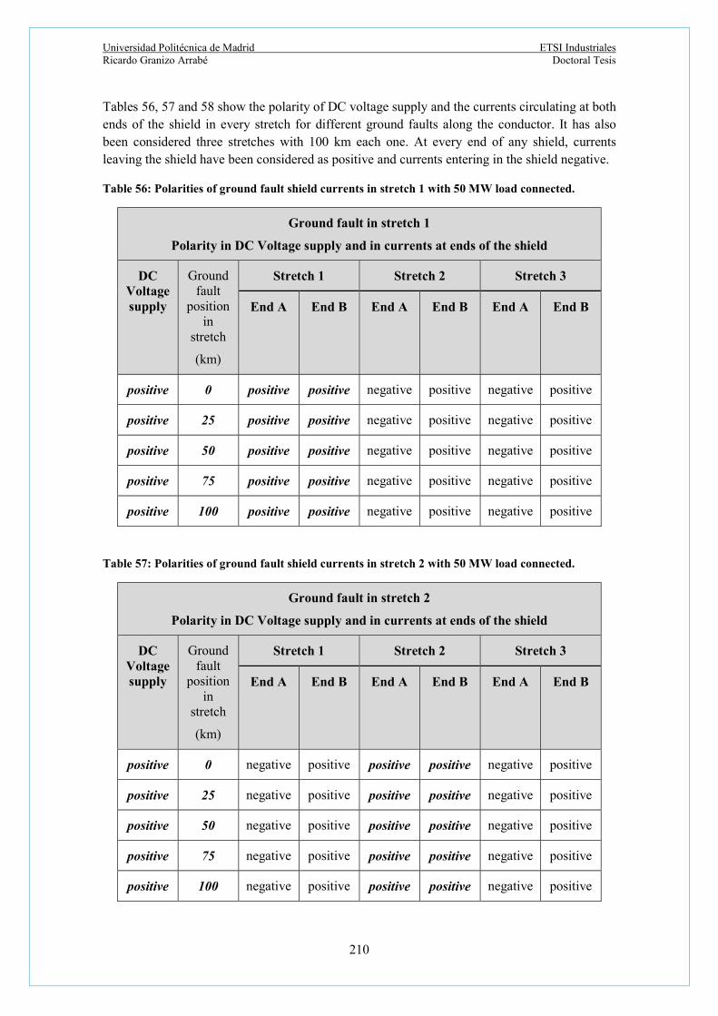
Universidad Politécnica de Madrid ETSI Industriales Ricardo Granizo Arrabé Doctoral Tesis
210
Tables 56, 57 and 58 show the polarity of DC voltage supply and the currents circulating at both ends of the shield in every stretch for different ground faults along the conductor. It has also been considered three stretches with 100 km each one. At every end of any shield, currents leaving the shield have been considered as positive and currents entering in the shield negative.
Table 56: Polarities of ground fault shield currents in stretch 1 with 50 MW load connected.
Ground fault in stretch 1
Polarity in DC Voltage supply and in currents at ends of the shield
DC Voltage supply
Ground fault
position in
stretch
(km)
Stretch 1 Stretch 2 Stretch 3
End A End B End A End B End A End B
positive 0 positive positive negative positive negative positive
positive 25 positive positive negative positive negative positive
positive 50 positive positive negative positive negative positive
positive 75 positive positive negative positive negative positive
positive 100 positive positive negative positive negative positive
Table 57: Polarities of ground fault shield currents in stretch 2 with 50 MW load connected.
Ground fault in stretch 2
Polarity in DC Voltage supply and in currents at ends of the shield
DC Voltage supply
Ground fault
position in
stretch
(km)
Stretch 1 Stretch 2 Stretch 3
End A End B End A End B End A End B
positive 0 negative positive positive positive negative positive
positive 25 negative positive positive positive negative positive
positive 50 negative positive positive positive negative positive
positive 75 negative positive positive positive negative positive
positive 100 negative positive positive positive negative positive

Universidad Politécnica de Madrid ETSI Industriales Ricardo Granizo Arrabé Doctoral Tesis
211
Table 58: Polarities of ground fault shield currents in stretch 3 with 50 MW load connected.
Ground fault in stretch 3
Polarity in DC Voltage supply and in currents at ends of the shield
DC Voltage supply
Ground fault
position in
stretch
(km)
Stretch 1 Stretch 2 Stretch 3
End A End B End A End B End A End B
positive 0 negative positive negative positive positive positive
positive 25 negative positive negative positive positive positive
positive 50 negative positive negative positive positive positive
positive 75 negative positive negative positive positive positive
positive 100 negative positive negative positive positive positive
Simulations without any load have been developed and their results are identical as shown in Tables 56, 57 and 58. Polarities of currents in the shields and DC voltage supply are the same when there is any load connected or not. Modulus of currents in shields before a defect happens are very small compared to the values of those currents when there is a fault. In these simulations the prefault shield currents modules are close to 50 A. However, the fault module currents in shields reach values from 7 to 16 kA. All these results give good evidence of the discrimination of the stretch where the ground fault was placed.
5.4.4. Experimental results: Ground fault.
The experimental set-up is the same as illustrated in 5.3.4. Different ground fault tests at positions A, B, C and D in the layout shown in previous Fig. 136 were performed with resistive loads from 0 to 150 Ω. Fig. 142 shows the ground fault currents for a defect in position B from positive conductor to the corresponding shield with 1 A load current.

Universidad Politécnica de Madrid ETSI Industriales Ricardo Granizo Arrabé Doctoral Tesis
212
Fig. 142: Ground fault currents with 150 Ω load connected.
Table 59: Polarities of ground fault shield currents with 27 Ω load connected.
Ground fault in stretch 1
Polarity in DC Voltage supply and in currents at ends of the shield
DC Voltage supply
Ground fault
position in
stretch
(km)
Stretch 1 Stretch 2 Stretch 3
End A End B End A End B End A End B
positive a positive positive negative positive negative positive
positive b positive negative negative positive negative positive
positive c positive negative positive negative negative positive
positive d positive negative positive negative positive positive
5.5. Identification of switching-on currents in DC insulated cables.
This research presents an identification method for detection of switching-on currents that allows distinguishing between fault and switching-on currents in shields of DC cables that have their shields grounded at both ends [143]. It is so the cable that has a ground fault is identified by analyzing the features of the currents at the ends of the shields of the cables and comparing such values to specific thresholds as well as to their oscillating characteristics. If the modules of the currents at both ends of the shield of a DC cable have values over a reference value and
-0.005 0 0.005 0.01 0.015 0.02 0.025 0.03-0.5
0
0.5
1
1.5
2
2.5
3
3.5
Time (s)
Cu
rre
nts
(A
)
Ground fault currents with load connected
CH1: Current in conductorCH3: Current in shield - Load sideCH4: Current in shield - DC Power Supply Side

Universidad Politécnica de Madrid ETSI Industriales Ricardo Granizo Arrabé Doctoral Tesis
213
there are no oscillations, the DC cable has a defect. Whenever there is no defect, the current presents oscillations until reaching its steady state. Therefore the discrimination between the currents corresponding to fault and switching-on actions is achieved. This way, false tripping commands are eliminated.
5.5.1. Description of the method.
This method identifies on the basis of the characteristics of the currents measured on cable screens, if such currents circulate through the screens correspond to energization maneuvers of the cables or defect situations. In the case of connection maneuvers, the currents read have the following characteristics:
a. They take positive and negative values until their complete attenuation.
b. So sign oscillations appear in their derivative with respect to time until their complete attenuation.
In the case of a defect in the cable, the measured currents present the following characteristics:
1. There aren´t variations in their signs.
2. Therefore, there are no oscillations in the sign of its derivative with respect to time.
In short, the detection of the ground fault is made by checking that the current in the cable screen with defect is higher than an adjustable threshold that has been previously adjusted by a predefined time, and whose adjusted threshold will depend on the value of the current on the screen.
In addition, the threshold previously adjusted for a certain time, must overcome the current in the screen of the isolated cable based on an expression that relates time and current, so that the greater the current of the effect, the shorter the tripping time. Also, it should be noted that only a defect in a cable will be considered, if the current on the corresponding screen does not show changes of sign during a defined time threshold, or if the derivative with respect to the time of the current on the screen does not show sign changes during a defined time threshold.
It is also important to consider the fact that by circulating an current along the screen of a cable without defect due to a defect that occurs in another cable, the blocking of the tripping of the cable without defect is related to the sign of the derivative of the current that circulates through the corresponding screen. It has opposite sign to the derivative of the current of the screen of the defective cable during a defined time threshold. Blocking of tripping is also possible when the derivative of the current with respect to the time in the isolated cable without defect, presents positive and negative slopes.

Universidad Politécnica de Madrid ETSI Industriales Ricardo Granizo Arrabé Doctoral Tesis
214
5.5.2. Simulation results: Switching-on currents in DC insulated cables.
The simulation circuit used to give evidence for this identification of switching-on currents method is the same as employed for the differential and directional ground fault detection methods.Simulations have shown the next values for the currents circulating in the shield when switching on commands take place. A 50 MW load was connected from the beginning. Fig. 143 shows the trends of such currents circulating at both ends of the cable set in operation.
Fig. 143: Switching-on currents in shields of a cable 220 kVdc with 50 MW load.
Simulations results for switching-on commands with 50 MW load are listed in Table 60. Such simulations show how up to 300 km cable length, the maximum current at the end of the shield close to the power supply with 50 MW load reaches 6.159 times the full load current value which is 227.27 A. On the other hand, oscillations remain stable from 175 km to 300 km cable length. Next simulations show the values for the currents circulating in the shield when switching on commands take place. This time, no load was connected from the beginning.
0 0.1 0.2 0.3 0.4 0.5 0.6 0.7 0.8 0.9 1-1500
-1000
-500
0
500
1000
1500
2000
Time (s)
Sw
itch
ing
curr
en
ts in
sh
ield
s (A
)
Switching currents in shields - 220 kVdc conductor with 50 MW load
Switching current in shield at the left endSwitching current in shield at the right end

Universidad Politécnica de Madrid ETSI Industriales Ricardo Granizo Arrabé Doctoral Tesis
215
Table 60: Switching-on shield currents with 50 MW load connected.
Peak value shield end close to power supply
(A)
Cable length
(km)
Peak value shield end away to power supply
(A)
Oscillating currents
851.91 100 639.03 YES
927.62 125 704.61 YES
999.56 150 775.69 YES
1067.51 175 840.51 YES
1127.64 200 889.86 YES
1187.17 225 946.88 YES
1239.11 250 989.70 YES
1291.51 275 1038.56 YES
1339.98 300 1082.75 YES
Fig. 144: Switching-on waveform currents in shields of a cable 220 kVdc without load connected.
Simulations results for switching-on commands without any load connected are listed in Table 61.
0 0.1 0.2 0.3 0.4 0.5 0.6 0.7 0.8 0.9 1-2000
-1500
-1000
-500
0
500
1000
1500
2000
Time (s)
Sw
itch
ing
curr
en
ts in
sh
ield
s (A
)
Switching currents in shields in 220 kVdc - No load connected.
Switching current at the shield - right sideSwitching current at the shield - left side
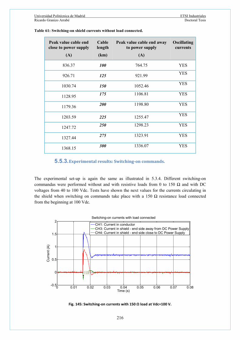
Universidad Politécnica de Madrid ETSI Industriales Ricardo Granizo Arrabé Doctoral Tesis
216
Table 61: Switching-on shield currents without load connected.
Peak value cable end close to power supply
(A)
Cable length
(km)
Peak value cable end away to power supply
(A)
Oscillating currents
836.37 100 764.75 YES
926.71 125 921.99 YES
1030.74 150 1052.46 YES
1128.95 175 1106.81 YES
1179.36 200 1198.80 YES
1203.59 225 1255.47 YES
1247.72 250 1298.23 YES
1327.44 275 1323.91 YES
1368.15 300 1336.07 YES
5.5.3. Experimental results: Switching-on commands.
The experimental set-up is again the same as illustrated in 5.3.4. Different switching-on commandas were performed without and with resistive loads from 0 to 150 Ω and with DC voltages from 40 to 100 Vdc. Tests have shown the next values for the currents circulating in the shield when switching on commands take place with a 150 Ω resistance load connected from the beginning at 100 Vdc.
Fig. 145: Switching-on currents with 150 Ω load at Vdc=100 V.
0 0.01 0.02 0.03 0.04 0.05 0.06 0.07 0.08-0.5
0
0.5
1
1.5
2
X: 0.0158Y: -0.127
Time (s)
Cu
rre
nt
(A)
Switching-on currents with load connected
CH1: Current in conductorCH3: Current in shield - end side away from DC Power SupplyCH4: Current in shield - end side close to DC Power Supply

Universidad Politécnica de Madrid ETSI Industriales Ricardo Granizo Arrabé Doctoral Tesis
217
Table 62 includes the tests results for switching-on commands with loads from 27.10 to 150 Ω and voltages from 40.62 to 100.20 Vdc.
Table 62: Switching-on shield currents with load connected.
DC Voltage
(V)
Load
(Ω)
Peak value shield end
close to power supply
(A)
Cable length
(m)
Peak value shield end
away to power supply
(A)
Oscillations
100.2 150
0.892 300 0.287 YES
0.881 300 0.283 YES
0.896 300 0.290 YES
0.890 300 0.288 YES
38.98 108.50
0.361 300 0.156 YES
0.332 300 0.143 YES
0.301 300 0.130 YES
0.314 300 0.134 YES
40.69 80.50
0.390 300 0.169 YES
0.421 300 0.182 YES
0.393 300 0.169 YES
0.403 300 0.175 YES
40,75 54.40
0.542 300 0.234 YES
0.511 300 0.221 YES
0.544 300 0.235 YES
0.527 300 0.229 YES
40.62 27.10
0.692 300 0.304 YES
0.721 300 0.313 YES
0.694 300 0.302 YES
0.744 300 0.323 YES

Universidad Politécnica de Madrid ETSI Industriales Ricardo Granizo Arrabé Doctoral Tesis
218
Next tests show the values for the currents circulating in the shield when switching on commands take place. This time, no load was connected from the beginning.
Fig. 146: Switching-on currents without any load connected.
Fig. 147: Switching-on current in shield without any load connected.
0.015 0.016 0.017 0.018 0.019 0.02 0.021 0.022 0.023 0.024 0.025-0.5
0
0.5
1
1.5
Time (s)
Cur
ren
t (A
)
Switching on currents with no load connected
CH1: Current in conductorCH4: Current in shield - end side away from DC Power SupplyCH3: Current in shield - end side near to DC Power Supply
4.4 4.6 4.8 5 5.2 5.4 5.6 5.8 6 6.2
x 10-6
-0.8
-0.6
-0.4
-0.2
0
0.2
0.4
0.6
0.8
1
Time (microseconds)
No
-lo
ad
sw
itch
-on
curr
en
t in
sh
ield
(A
)
Switch-on current in shield

Universidad Politécnica de Madrid ETSI Industriales Ricardo Granizo Arrabé Doctoral Tesis
219
Table 62: Switching-on conductor currents without load connected.
Peak value shield end
close to power supply
(A)
Cable length
(m)
Peak value shield end away to power supply
(A)
Oscillations
0.902 300 0.287 YES
0.905 300 0.288 YES
0.904 300 0.288 YES
1.081 300 0.344 YES
0.901 300 0.284 YES
5.6. Glossary fifth chapter.
f Frequency Gi Generation system i HVDC High voltage direct current εcs Relative permittivity conductor-shield εse Relative permittivity shield ρAl Resistivity of Aluminium ΡCu Resistivity of Copper ρe Ground resistivity

Universidad Politécnica de Madrid ETSI Industriales Ricardo Granizo Arrabé Doctoral Tesis
220
Universidad Politécnica de Madrid ETSI Industriales Ricardo Granizo Arrabé Doctoral Tesis
221
6. CONCLUSIONS AND FUTURE LINES OF
RESEARCH

Universidad Politécnica de Madrid ETSI Industriales Ricardo Granizo Arrabé Doctoral Tesis
222
his chapter summarizes the most relevant conclusions of this Doctoral Thesis. At the end there is a list of the patents and articles developed during the doctoral period. New concepts and methods for protection systems in ac networks have been defined,
simulated and tested in the laboratory of Electrical Machines inside the Electrical Engineering Department of ETSII. Some patents for DC power systems have been obtained as result of a common research for improvements in cable protection methods and systems.
6.
T

Universidad Politécnica de Madrid ETSI Industriales Ricardo Granizo Arrabé Doctoral Tesis
223
6.1. Conclusions.
The main conclusions from the new algorithm for blocking the auto-reclosing developed for AC combined overhead-cable lines that can be drawn are:
Development of a new algorithm that increases the accuracy in the determination of the position of ground faults in combined overhead-cable lines. Results from 1 m ahead from the transition overhead-cable in both directions have shown good results.
Development of a new algorithm that improves the auto-reclosing maneuvers to avoid reconnecting overhead-cable lines with active ground fault conditions. As result of a precise location of the ground fault, the power system is not exposed to unsuccessful reclosing attempts with the consequent improvement in the life of the power elements of the system.
o The reduction of wrong reclosings improves the power system stability because unsuccessful auto-reclosing commands are eliminated. Therefore power oscillations between synchronous generators are reduced to the inherent oscillations when ground faults happen in the system.
o The reduction of wrong reclosings orders reduces damages in cables and improves the cable protection due to the fact that there are no seconds or thirds auto-reclosing attempts if the ground fault has been classified as cable ground fault. Severe damages in cables as consequence of switching them on fault are knocked out
Application of Wavelet transformation is a valid tool for ground fault detection and location.
Standard and classical current transformers can be used for all these improvements in protection systems. It is important to highlight that no special sensors for high frequency measurements are needed so typical applications of them are considered.
Current measurements are only made at one end of the cable placed at the substation side, not at the transition overhead-cable station. This important fact makes easier to detect and locate ground faults as no physical connection by FO cable between devices at both cable ends are required. Also, a price reduction with higher protection performances is obtained.
Voltage measurements are not needed in these protection improvements. The necessity of installing voltage transformers for protection purposes is avoided as no directional features are requested or voltage increases or decreases are considered.
The measurements of currents on each conductor and on each shield allow determining the location of the ground fault. Normally, there are no current transformers measuring only current in shields so it use for measuring such currents allows increasing the protection performances for cable protection in general applications and also for reclosing commands improvements.

Universidad Politécnica de Madrid ETSI Industriales Ricardo Granizo Arrabé Doctoral Tesis
224
The main conclusions from the Novel Protection Method for Detection of Ground Faults in Cables Used in Combined Overhead-Cable Lines in Power Systems that can be drawn are:
Development of a new method for detection of ground faults in cables used in combined overhead-cable lines in power systems that only measures currents in the shields of the cables and allows determining where the ground fault happened by means of analyzing their modulus and angles.
Development of new protection system that evaluates the changes in the differences between angles of currents in conductors and in shields in function of the topology of shield connections.
The calculation of the covariance between the values of the modules of the intensities in the shields and their respective angles allows detecting if the cable has ground fault or not with an accuracy of 1 m, either from the transition to the cable side or to the line side.
Reductions of costs in protection systems used in combined overhead-cable lines, either for transmission or distribution networks. Standard ring core current transformers and a new protection relay that includes these new methods is a low budget investment for the problems that can clear in the power system.
The main conclusions from the Novel Ground Fault Non Directional Selective Protection Method for ungrounded distribution networks that can be drawn are:
Development of a new selective non-directional tripping criterion for main substations. The switchgear or position where the capacitive ground fault current value is higher is the line where there is a ground defect.
Developmenty of a new selective non-directional tripping criterion for secondary substations. The incoming capacitive defect current in the secondary substation is compared to the outgoing capacitive defect current. If both values are equal, the defect is located in other line or in other substation. If not, the line that has maximum capacitive defect current is the line with ground defect.
The main conclusions from the New Differential Ground Fault Detection Method for DC Insulated Cables that can be drawn are:
Development of a new differential method to detect which cable has a ground defect in a multiterminal cable DC network. This method measures the currents at the ends of the shields and evaluates their modulus and polarities:
o Any cable with ground defect has currents circulating at both ends of its shield with values over a reference threshold with identical polarities.
o Any cable without ground defect has currents circulating at both ends of its shield with different polarity.

Universidad Politécnica de Madrid ETSI Industriales Ricardo Granizo Arrabé Doctoral Tesis
225
The main conclusions from the New Directional Ground Fault Detection Method for DC Insulated Cables that can be drawn are:
Development of a New Directional Ground Fault Detection Method to detect which cable has a ground defect in a multiterminal cable DC network that measures the polarity of currents in shields and the main conductors as well as their modulus:
o Any cable that has a ground fault has intensities circulating at the ends of its shield with values over a defined threshold with the same polarity as the main conductor during a previous set time.
o Any cable without ground defect has intensities circulating at the ends of its shield with values over a defined threshold with different polarity than the main conductor at least at one end of the shield during a time set frame.
The main conclusions from the New Method for Identification of Switching-On Currents in DC insulated cables that can be drawn are:
Development of a new method that differentiates between connection or inrush currents and ground defect intensities if the current measured in shields is higher than a threshold during a time.
Development of a new method that detects connection or inrush currents if the current waveforms on the cable screens have positive and negative slopes in a time interval, the cable has no defect.
Development of a new method that detects cables with ground faults if the currents measured during a time interval always have a positive or negative slope.

Universidad Politécnica de Madrid ETSI Industriales Ricardo Granizo Arrabé Doctoral Tesis
226
6.2. Future lines of research.
The performances of protection systems can look further and achieve new challenges. Some of them are indicated below:
1. The research of the use of high frequency current transformers/sensors: It might be interesting to research with high frequency sensors and be able to obtain the location of ground faults in the range of 1 – 2 ms. If so, using the standard communication protocol IEC61850 might be a breakthrough in the coordination of protection function placed at different substations.
2. The research for obtaining the exact ground fault position measuring only currents in shields of power cables in only one end: So far all methods described in this Doctoral Thesis and the up and running methods applied to protection relays already in service can´t obtain such position.
3. The research of ground faults location using statistics variables: Statistic allows establishing and finding relations between fault currents that can improve protections methods for localization of the ground fault position. Covariance calculations have been used in this Doctoral Thesis with outstanding results for discrimination the fault zone in combined overhead-cable lines.
6.3. Publications.
The main contributions related to the work developed along this doctoral period are three articles published in journals indexed in the "Journal Citation Report (JCR)", one patent licensed for commercial purposes to a Spanish company and another six patents.
1.- Title: A Novel Ground Fault Non-Directional Selective Protection
Method for Ungrounded Distribution Networks Type of contribution:
Magazine.
Name: Energies Year: 2015. Summary: This paper presents a new selective and non-directional protection
method to detect ground faults in ungrounded power systems. The new proposed method is based on the comparison of the rms value of the residual current of all the lines connected to a bus, and it is able to determine the line with ground defect. Additionally, this method can be used for the protection of secondary substation. This protection method avoids the unwanted trips produced by wrong settings or wiring errors, which sometimes occur in the existing directional ground fault protections.

Universidad Politécnica de Madrid ETSI Industriales Ricardo Granizo Arrabé Doctoral Tesis
227
2.- Title: Novel Auto-Reclosing Blocking Method for Combined Overhead-Cable Lines in Power Networks
Type of contribution:
Magazine.
Name: Energies Year: 2016. Summary: This paper presents a novel auto-reclosing blocking method
for combined overhead-cable lines in power distribution networks that are solidly or impedance grounded, with distribution transformers in a delta connection in their high-voltage sides. The main contribution of this new technique is that it can detect whether a ground fault has been produced at the overhead line side or at the cable line side, thus improving the performance of the auto-reclosing functionality. This localization technique is based on the measurements and analysis of the argument differences between the load currents in the active conductors of the cable and the currents in the shields at the cable end where the transformers in delta connection are installed, including a wavelet analysis.
3.- Title: Novel Protection Method for Detection of ground Faults in
Cables Used in Combined Overhead-Cable Lines in Power Systems
Type of contribution:
Conference
Name: IEEE 17th International Conference on Environment and Electrical Engineering and 1st Industrial and Commercial Power Systems Europe
Year: 2017 Summary: This paper presents a new protection method for ground faults
detection in cables used in overhead-cable lines in power transmission systems where the shields of the cables are connected according to the cross-bonding method The main contribution of this new protection method is that it can distinguish ground faults in the cable line side from ground faults at the overhead-line side. The new protection method is based on the measurements and analysis of the currents in the shields of the conductors at the cable end at the substation side, not at the cable end in the transition overhead-cable. The new method considers that the shields of the cables at the transition overhead-cable are not grounded sharing the same ground than the ending tower. Shields of the cables are connected according to the cross-bonding method.
4.- Title: Method and System of Ground Fault Discrimination in
Circuits with Transitions Overhead-Cable Type of contribution:
Patent
Name: P201100343 Year: 04/06/2014 Summary: Method and system of discrimination of ground faults in circuits
Universidad Politécnica de Madrid ETSI Industriales Ricardo Granizo Arrabé Doctoral Tesis
228
with overhead-cable transitions. The present invention is a novel system for reclose locking for single-phase faults in electrical networks that have transitions overhead - cable in which said cables have their shields grounded in a single point. This system discriminates if the single-phase ground fault has occurred on the overhead or cable sides. In basis of this discrimination, the system will allow the reclosing command if the fault has occurred on the overhead side or block such reclosing if the fault has been produced in the cable side. This invention is addressed to electrical distribution networks with star points rigidly grounded or through impedance.
5.- Title: Method of Determining the Location where a Single-Phase
Ground Fault Occurs in Circuits with Transitions Overhead - Underground Cable
Type of contribution:
Patent licensed to the company DSF-TECNOLOGÍAS PARA MOTORES for commercial use.
Name: P201431962 Year: 22/09/2015 Summary: Method of determining the position where a ground fault occurs
in circuits with transitions overhead - underground cable, where the shields of the underground cables are connected in a transposed and grounded manner in both ends. Basically it comprises:
- Reception a trigger signal from one of the line protections with underground – overhead sides.
- Evaluation the relationships between the modules of the currents that circulate on the screens of the power cables, direct sequence and zero on the one hand, and inverse and zero by other.
- Evaluation of the angular differences between currents circulating on said shields.
- Comparison of the relationships between the modules of currents with a reference module value X, and the angular differences with an angular value of reference Z.
- Following the comparisons said before, the reclosing maneuver is allowed or blocked.
6.- Title: Method and Directional Detection System for Ground Faults
in DC Networks with insulated cables Type of
contribution: Patent
Name: P201431916 Year: 30/09/2016 Summary: Ground fault detection method and system for dc cable networks
which comprises at least one shield grounded, a measuring equipment of current flowing on the shield which obtains a current measurement signal, an analyzer device of the measurement signal and a current adjusting signal that circulates in the shield, which in turn comprises:
- Means for obtaining a polarity value of current and a signal value of such current.
- A divider which compares the strength of the signal of the current measured with a previous current setting value.

Universidad Politécnica de Madrid ETSI Industriales Ricardo Granizo Arrabé Doctoral Tesis
229
- A comparator that compares the polarity of current with a definite polarity sign previously defined.
- Means for generating a tripping signal which indicates a defect in the cable from the output signals of the divider and the comparator.
7.- Title: Differential Ground Fault Detection Method and System for
DC insulated cables Type of
contribution: Patent
Name: P201431014 Year: 05/05/2015 Summary: The present invention relates to a novel method and system for
selective detection of ground faults in DC cables that have their shields grounded at both ends. The cable that has a ground fault is identified by measuring the currents of the defect at the ends of the two cable shields. These two currents have opposite polarity if the cable is not faulty. On the other hand, if the cable is defective, the two currents have equal polarities. It also knows and identifies the cable with ground fault by measuring and comparing the currents that circulate at the two ends of the shield. This invention is capable of discriminating between the currents corresponding to the maneuvers of connection of protected cables and the corresponding currents with ground faults. This way, erroneous or improper tripping commands are eliminated.
8.- Title: Non-Directional Protection System and Method for Selective
Detection of Ground Faults in Ungrounded Networks Type of
contribution: Patent
Name: P201000510 Year: 31/01/2013 Summary: Single phase detection system and method to detect ground faults
in electrical power grids with star point ungrounded or with high impedance value, which offers total selectivity in the detection of the area in fault situation and is based in the comparison of the modules of the zero currents of the lines, being the line with defect the one which has the highest current. In electrical systems with secondary substations, it is determined whether the defect is in the secondary substation through the comparison of the sum of the modules of the incoming currents of the power lines to the currents in the outgoing lines. If there is a failure in the secondary substation, the faulty line is determined because its zero current is the largest of all outgoing lines.
9.- Title: Method and Protection System for Ungrounded Electrical
Grids Type of
contribution: Patent
Name: P201230777 Year: 09/06/2014 Summary: This invention is a novel method and system detection of ground
faults in ungrounded or high impedance grounding electrical distribution grids. The line that has a single-phase fault is identified based on directional comparisons between all the defect
Universidad Politécnica de Madrid ETSI Industriales Ricardo Granizo Arrabé Doctoral Tesis
230
currents that circulate in the lines in service and a reference current.
10.- Title: Ground Detection Method and System in DC Networks with
Insulated Cables Type of
contribution: Patent
Name: P201431003 Year: 30/10/2015 Summary: The present invention relates to a method and a system for
selective detection of ground faults in DC networks made up of insulated cables that have their shields grounded in at least one of its two ends. It identifies the cable that has a ground defect by measuring analyzing the currents that circulate in the shields of the cables. These defect currents that circulate in the screens can be measured in various ways. This patent tries to solve the problem of detecting a ground fault selectively in networks with insulated cables in DC power systems. It has the advantage that the current measurement in the shields is simpler than in the own conductor, since the insulation voltage required for the measuring equipment is much lower than measuring in the cable.
Universidad Politécnica de Madrid ETSI Industriales Ricardo Granizo Arrabé Doctoral Tesis
231
References.
Universidad Politécnica de Madrid ETSI Industriales Ricardo Granizo Arrabé Doctoral Tesis
232
[1] Saha, M.M.; Izykowsky, J; Rosolowsky, E. Fault Location on Power Networks. Springer Verlag. Berlin, 2009.
[2] Horowitz, S. H.; Phadke, A.G. Power System Relaying, Third Edition. Wiley. New York, 2008.
[3] Li, P.; Zhang, B.H.; Hao, Z.G.; Rao, Y.F.; Wang, Y.T.; Bo, Z.Q.; Klimek, A.; Zhao, Q.; He, W. Optimal Reclosing Time of Transmission Lines and its Application in Real Power System. Presented at the Developments in Power System Protection 9th International Conference, March 2008, vol. 110, no. 115, pp. 17-20.
[4] He Renwang, "A New Approach to the Calculation of Reclosing Time for Adaptive Auto-reclosure," in Power and Energy Engineering Conference (APPEEC), 2010 Asia-Pacific , vol., no., pp.1-2, 28-31 March 2010 doi: 10.1109/APPEEC.2010.5448457
[5] Jamali, S.; Parham, A., "New approach to adaptive single pole auto-reclosing of power transmission lines," Generation, Transmission & Distribution, IET , vol.4, no.1, pp.115,122, January 2010
[6] V. H. Makwana and B. R. Bhalja, "A New Digital Distance Relaying Scheme for Compensation of High-Resistance Faults on Transmission Line," in IEEE Transactions on Power Delivery, vol. 27, no. 4, pp. 2133-2140, Oct. 2012. doi: 10.1109/TPWRD.2012.2202922
[7] Su Sheng, Liu Jianhua, Xiao Hui and Jiang Dongjun, "Expert System for Wide Area Protection Zone Selection," 2005 IEEE/PES Transmission & Distribution Conference & Exposition: Asia and Pacific, Dalian, 2005, pp. 1-3. doi: 10.1109/TDC.2005.1547054
[8] P. Pierz, E. Rosolowski, J. Izykowski, P. Balcerek and M. M. Saha, "A method for internal and external fault discrimination for protection of series compensated double-circuit line," 2013 IEEE Grenoble Conference, Grenoble, 2013, pp. 1-6. doi: 10.1109/PTC.2013.6652404
[9] S. J. Jung and I. S. Kang, "Protection relay stability study for 115kV and 34.5kV transmission and distribution system," 2011 International Conference on Advanced Power System Automation and Protection, Beijing, 2011, pp. 1060-1064. doi: 10.1109/APAP.2011.6180533
[10] P. Crossley and J. Pugh, "Measuring the reliability of a protection scheme used for fault clearance on a transmission feeder," IEE Colloquium on The Impact of Protection and Control on Quality of Supply (Digest No: 1997/357), Glasgow, 1997, pp. 4/1-4/6. doi: 10.1049/ic:19971189
[11] W. Gai, W. Cong, Z. Zhang, Z. Zhang, J. Xiao and Y. Feng, "Research on distributed wide-area back-up protection system for high-voltage transmission system," 2016 IEEE

Universidad Politécnica de Madrid ETSI Industriales Ricardo Granizo Arrabé Doctoral Tesis
233
PES Asia-Pacific Power and Energy Engineering Conference (APPEEC), Xi'an, 2016, pp. 1269-1273. doi: 10.1109/APPEEC.2016.7779697
[12] B. Kasztenny et al., "Exploring the IEEE C37.234 Guide for Protective Relay Application to Power System Buses," in IEEE Transactions on Power Delivery, vol. 26, no. 2, pp. 936-943, April 2011. doi: 10.1109/TPWRD.2010.2048128
[13] DBT. Digital Trip Coil Supervision Relay. Instruction manual. GE publication code: GEK-105597E, December 2016.
[14] S. F. Tan and S. K. Salman, "Application of single pole auto reclosing in distributaion networks with high pentration of DGS," 2009 44th International Universities Power Engineering Conference (UPEC), Glasgow, 2009, pp. 1-5.
[15] J. Li, Y. Qi, Q. Gao and S. Sun, "Single phase to ground fault location based on phase of zero-sequence current," 2013 IEEE International Conference on Information and Automation (ICIA), Yinchuan, 2013, pp. 856-859. doi: 10.1109/ICInfA.2013.6720413
[16] S. Mangione, "A Simple Method for Evaluating Ground-Fault Current Transfer at the Transition Station of a Combined Overhead-Cable Line," in IEEE Transactions on Power Delivery, vol. 23, no. 3, pp. 1413-1418, July 2008.doi: 10.1109/TPWRD.2007.915895
[17] M. H. Idris, M. W. Mustafa and Y. Yatim, "Effective two-terminal single line to ground fault location algorithm," 2012 IEEE International Power Engineering and Optimization Conference Melaka, Malaysia, Melaka, 2012, pp. 246-251. doi: 10.1109/PEOCO.2012.6230869
[18] B. Wang, X. Dong, L. Lan and F. Xu, "Novel location algorithm for single-line-to-ground faults in transmission line with distributed parameters," in IET Generation, Transmission & Distribution, vol. 7, no. 6, pp. 560-566, June 2013. doi: 10.1049/iet-gtd.2012.0379
[19] R. Nandi and B. K. Panigrahi, "Detection of fault in a hybrid power system using wavelet transform," Michael Faraday IET International Summit 2015, Kolkata, 2015, pp. 203-206. doi: 10.1049/cp.2015.1631
[20] F. B. Costa, A. Monti and S. C. Paiva, "Overcurrent Protection in Distribution Systems With Distributed Generation Based on the Real-Time Boundary Wavelet Transform," in IEEE Transactions on Power Delivery, vol. 32, no. 1, pp. 462-473, Feb. 2017. doi: 10.1109/TPWRD.2015.2509460
[21] M. N. Mahmud, M. N. Ibrahim, M. K. Osman and Z. Hussain, "Selection of suitable features for fault classification in transmission line," 2015 IEEE International Conference on Control System, Computing and Engineering (ICCSCE), George Town, 2015, pp. 591-596. doi: 10.1109/ICCSCE.2015.7482253

Universidad Politécnica de Madrid ETSI Industriales Ricardo Granizo Arrabé Doctoral Tesis
234
[22] Diao-Yan Hua, Li-Chun Ming and Shang Yan, "Wavelet-based fault diagnosis scheme for power system relay protection," 2008 International Conference on Machine Learning and Cybernetics, Kunming, 2008, pp. 2187-2191. doi: 10.1109/ICMLC.2008.4620768
[23] D. Yanhua, W. Shuhai, P. Zhifeng and Li Yuping, "Reserch on Extracting the Features at Relay Protection Based on Wavelet Transform Modulus Maximum," 2007 8th International Conference on Electronic Measurement and Instruments, Xi'an, 2007, pp. 2-555-2-558. doi: 10.1109/ICEMI.2007.4350741
[24] G. Sudha and T. Basavaraju, "A comparison between different approaches for fault classification in transmission lines," 2007 IET-UK International Conference on Information and Communication Technology in Electrical Sciences (ICTES 2007), Tamil Nadu, 2007, pp. 398-403.
[25] H. Livani and C. Y. Evrenosoglu, "A traveling wave based single-ended fault location algorithm using DWT for overhead lines combined with underground cables," IEEE PES General Meeting, Providence, RI, 2010, pp. 1-6. doi: 10.1109/PES.2010.5590150
[26] A. Sharafi, P. Jafarian and M. Sanaye-Pasand, "A combined algorithm for high speed transmission-line protection based on traveling-wave," 2010 9th International Conference on Environment and Electrical Engineering, Prague, Czech Republic, 2010, pp. 132-135. doi: 10.1109/EEEIC.2010.5489973
[27] S. Beheshtaein, M. Savaghebi, J. C. Vasquez and J. M. Guerrero, "A hybrid algorithm for fault locating in looped microgrids," 2016 IEEE Energy Conversion Congress and Exposition (ECCE), Milwaukee, WI, 2016, pp. 1-6. doi: 10.1109/ECCE.2016.7855166
[28] Hosung Jung, Young Park, Moonseob Han, Changmu Lee, Hyunjune Park, Myongchul Shin, Novel technique for fault location estimation on parallel transmission lines using wavelet, International Journal of Electrical Power & Energy Systems, Volume 29, Issue 1, 2007, Pages 76-82, ISSN 0142-0615, http://dx.doi.org/10.1016/j.ijepes.2006.05.002.
[29] A. Ngaopitakkul, C. Pothisarn, S. Bunjongjit and B. Suechoey, "An Application of Discrete Wavelet Transform and Support Vector Machines Algorithm for Classification of Fault Types on Underground Cable," 2012 Third International Conference on Innovations in Bio-Inspired Computing and Applications, Kaohsiung, 2012, pp. 85-88. doi: 10.1109/IBICA.2012.21
[30] Martínez, F.; Peris, A.; Rodenas, F. Tratamiento de Señales Digitales Mediante Wavelets y su uso con Matlab. Editorial Club Universitario. Alicante, 2004.
[31] Stucke GmbH, SYMAP_Compact_Manual_v20.0_GB.
[32] MRA4 HighPROTEC Feeder Protection, Device Manual.
[33] Standard EN61869-2: 2012. Instrument transformers. Additional requirements for

Universidad Politécnica de Madrid ETSI Industriales Ricardo Granizo Arrabé Doctoral Tesis
235
current transformers.
[34] Nisha Das and M. K. Kazimierczuk, "An overview of technical challenges in the design of current transformers," Proceedings Electrical Insulation Conference and Electrical Manufacturing Expo, 2005., Indianapolis, IN, 2005, pp. 369-377.doi: 10.1109/EEIC.2005.1566323
[35] H. E. Mostafa, A. M. Shalltoot and H. K. M. Youssef, "Evaluation of current transformer performance in the presence of remnant flux and harmonics," 2011 IEEE Jordan Conference on Applied Electrical Engineering and Computing Technologies (AEECT), Amman, 2011, pp. 1-6. doi: 10.1109/AEECT.2011.6132490
[36] Technical guide. Protection criteria for medium voltage networks. ABB S.p.A. Unità Operativa Sace-MV.
[37] MRI3-IE - Digital multifunctional relay for earth fault protection. January 2010. Woodward SEG GmbH & Co. KG
[38] Schneider: Protección de las redes eléctricas. Sepam serie 10, página 41.
[39] S. Couture, R. Chang, I. Volvach, A. Goncharov and V. Lomakin, "Coupled Finite Element Micromagnetic - Integral Equation Electromagnetic Simulator for Modeling Magnetization - Eddy Currents Dynamics," in IEEE Transactions on Magnetics, vol. PP, no. 99, pp. 1-1. doi: 10.1109/TMAG.2017.2745470
[40] Karl Hess, "A Brief Review of the Relevant Basic Equations of Physics," in Advanced Theory of Semiconductor Devices , 1, Wiley-IEEE Press, 2000, pp.1-18. doi: 10.1109/9780470544105.ch1.
[41] A. Ponniran and M. S. Kamarudin, "Study on the performance of underground XLPE cables in service based on tan delta and capacitance measurements," 2008 IEEE 2nd International Power and Energy Conference, Johor Bahru, 2008, pp. 39-43. doi: 10.1109/PECON.2008.4762442.
[42] Lirong Chen, Rong Xia and Junhua Luo, "Technique research on the online detection and restraint of the induced voltage and circulating current on the metal sheath of 35kV 630mm2 single-core XLPE cable," CICED 2010 Proceedings, Nanjing, 2010, pp. 1-6.
[43] W. Moutassem and G. J. Anders, "Calculation of the Eddy Current and Hysteresis Losses in Sheathed Cables Inside a Steel Pipe," in IEEE Transactions on Power Delivery, vol. 25, no. 4, pp. 2054-2063, Oct. 2010. doi: 10.1109/TPWRD.2010.2049509
[44] X. p. Kong, Y. x. Wang, Z. Zhang, X. g. Yin and X. Deng, "Calculation of induced voltage in metal shield of single-core cable operated in parallel," 2010 International Conference on Power System Technology, Hangzhou, 2010, pp. 1-8. doi: 10.1109/POWERCON.2010.5666157

Universidad Politécnica de Madrid ETSI Industriales Ricardo Granizo Arrabé Doctoral Tesis
236
[45] Y. Lin and Z. Xu, "Cable Sheath Loss Reduction Strategy Research Based on the Coupled Line Model," in IEEE Transactions on Power Delivery, vol. 30, no. 5, pp. 2303-2311, Oct. 2015. doi: 10.1109/TPWRD.2015.2414655
[46] N. Theethayi and R. Thottappillil, "On Reducing the Lightning Transients in Buried Shielded Cables Using Follow-On Earth Wire," in IEEE Transactions on Electromagnetic Compatibility, vol. 49, no. 4, pp. 924-927, Nov. 2007. doi: 10.1109/TEMC.2007.908259
[47] G. Ban, L. Prikler, I. Fogarasi and I. Hajos, "Protection of MV covered conductor lines against overvoltages and fault arcs," 2005 IEEE Russia Power Tech, St. Petersburg, 2005, pp. 1-7. doi: 10.1109/PTC.2005.4524646
[48] Cálculo y Diseño de Líneas Eléctricas de Alta Tensión, Pascual Simón Comín, Fernando garnacho Vecino, Jorge Moreno Mohíno, Alberto González Sanz. ISBN:978-84-9281-286-8. Editorial Garceta, 2011.
[49] IEEE Guide for the Application of Sheath-Bonding Methods for Single-Conductor Cables and the Calculation of Induced Voltages and Currents in Cable Sheaths," in ANSI/IEEE Std 575-1988 , vol., no., pp.0_1-, 1987. doi: 10.1109/IEEESTD.1987.122985
[50] Y. Du, X. H. Wang and Z. H. Yuan, "Induced Voltages and Power Losses in Single-Conductor Armored Cables," in IEEE Transactions on Industry Applications, vol. 45, no. 6, pp. 2145-2151, Nov.-dec. 2009. doi: 10.1109/TIA.2009.2031904
[51] Connection of earthing circuits in high voltage systems. General Cable, ICAT 2005.
[52] IEEE Guide for Bonding Shields and Sheaths of Single-Conductor Power Cables Rated 5 kV through 500 kV," in IEEE Std 575-2014 (Revision of IEEE Std 575-1988) , vol., no., pp.1-83, Sept. 18 2014. doi: 10.1109/IEEESTD.2014.6905681
[53] M. Mahdipour, A. Akbari, M. Khalilzadeh and P. Werle, "Impact of different bonding methods on high voltage cable shield induced voltage and current in normal and fault conditions," 2017 Iranian Conference on Electrical Engineering (ICEE), Tehran, 2017, pp. 1308-1312. doi: 10.1109/IranianCEE.2017.7985244
[54] S. Czapp, K. Dobrzynski, J. Klucznik and Z. Lubosny, "Impact of configuration of earth continuity conductor on induced sheath voltages in power cables," 2016 International Conference on Information and Digital Technologies (IDT), Rzeszow, 2016, pp. 59-63. doi: 10.1109/DT.2016.7557150.
[55] M. Shaban, M. A. Salam, S. P. Ang, M. Norfauzi, F. Wen and W. Voon, "Calculation of induced sheath voltage for transposed and untransposed cable conductors," TENCON 2015 - 2015 IEEE Region 10 Conference, Macao, 2015, pp. 1-6. doi: 10.1109/TENCON.2015.7372833

Universidad Politécnica de Madrid ETSI Industriales Ricardo Granizo Arrabé Doctoral Tesis
237
[56] Mingzhen Li et al., "A novel fault localization method based on monitoring of sheath current in a cross-bonded HV cable system," 2017 IEEE Electrical Insulation Conference (EIC), Baltimore, MD, 2017, pp. 123-126. doi: 10.1109/EIC.2017.8004678
[57] Effects of un-transposed UHV transmission line on fault analysis of power systems, Transactions of Tianjin University, June 2008, Volume 14, Issue 3, pp 231-234.
[58] IEEE Approved Draft Guide for Bonding Shields and Sheaths of Single-Conductor Power Cables Rated 5 kV through 500 kV," in IEEE P575/D13, May 2014 , vol., no., pp.1-82, Sept. 18 2014
[59] P. Nichols, "Minimum voltage rating of sheath voltage limiters in underground cable systems: The influence of corrugated cable sheaths," 2012 47th International Universities Power Engineering Conference (UPEC), London, 2012, pp. 1-6. doi: 10.1109/UPEC.2012.6398659
[60] J. A. Calvillo, J. R. Morales and F. A. Uribe, "Sensitivity analysis of ground impedances of power cables in electromagnetic transient responses," 2016 IEEE International Autumn Meeting on Power, Electronics and Computing (ROPEC), Ixtapa, 2016, pp. 1-6. doi: 10.1109/ROPEC.2016.7830607.
[61] L. Xu and M. Xue, "Selection of optimal wavelet basis for singularity detection of non-stationary signal," 2011 International Conference on Electrical and Control Engineering, Yichang, 2011, pp. 4959-4962. doi: 10.1109/ICECENG.2011.6057359
[62] Z. Wang, S. McConnell, R. S. Balog and J. Johnson, "Arc fault signal detection - Fourier transformation vs. wavelet decomposition techniques using synthesized data," 2014 IEEE 40th Photovoltaic Specialist Conference (PVSC), Denver, CO, 2014, pp. 3239-3244. doi: 10.1109/PVSC.2014.6925625.
[63] A. Borghetti, M. Bosetti, M. Di Silvestro, C. A. Nucci and M. Paolone, "Continuous-Wavelet Transform for Fault Location in Distribution Power Networks: Definition of Mother Wavelets Inferred From Fault Originated Transients," in IEEE Transactions on Power Systems, vol. 23, no. 2, pp. 380-388, May 2008. doi: 10.1109/TPWRS.2008.919249
[64] F. E. Perez, R. Aguilar, E. Orduna, J. Jager and G. Guidi, "High-speed non-unit transmission line protection using single-phase measurements and an adaptive wavelet: zone detection and fault classification," in IET Generation, Transmission & Distribution, vol. 6, no. 7, pp. 593-604, July 2012. doi: 10.1049/iet-gtd.2011.0592
[65] J. Romberg, "Sampling and reconstruction in the 21st century," 2017 IEEE International Conference on Acoustics, Speech and Signal Processing (ICASSP), New Orleans, LA, 2017, pp. 6468-6472. doi: 10.1109/ICASSP.2017.7953402
[66] Z. Xiaoguang, H. Bingrong and W. Donqmu, "Implementation of time-scale
Universidad Politécnica de Madrid ETSI Industriales Ricardo Granizo Arrabé Doctoral Tesis
238
transformation based on continuous wavelet theory," in Journal of Systems Engineering and Electronics, vol. 11, no. 1, pp. 32-37, March 2000.
[67] Mathworks, Wavelet toolbox Software, version 4.8, 2011.
[68] Yilmazlar, I., & Kokturk, G. (2010, May). Power system failure analysis by using the discrete wavelet transform. In 10th WSEAS International Conference on Wavelet Analysis and Multirate Systems (pp. 56-60).
[69] R. H. G. Tan and V. K. Ramachandaramurthy, "Capacitor bank switching classification using scale selection continuous wavelet transform," 2009 International Conference on Power Electronics and Drive Systems (PEDS), Taipei, 2009, pp. 950-955. doi: 10.1109/PEDS.2009.5385785
[70] Y. Long, "An approach to identify magnettizing inrush currents and its simulation," Proceedings of 2011 International Conference on Electronic & Mechanical Engineering and Information Technology, Harbin, Heilongjiang, China, 2011, pp. 2377-2380. doi: 10.1109/EMEIT.2011.6023588
[71] Wavelets and their Applications, Michael Misiti, ISTE Ltd, United States 2007, ISBN: 978-1-905209-31-6.
[72] M. C. Xia and Y. Z. Huang, "Wavelet analysis in transient based protection for power system high voltage transmission line," 2010 International Conference on Wavelet Analysis and Pattern Recognition, Qingdao, 2010, pp. 427-430. doi: 10.1109/ICWAPR.2010.5576409
[73] A. H. Osman and O. P. Malik, "Experimental test results for a parallel transmission lines protection scheme using wavelet transform," in IEE Proceedings - Generation, Transmission and Distribution, vol. 151, no. 6, pp. 713-720, 12 Nov. 2004. doi: 10.1049/ip-gtd:20041071
[74] J. Klomjit and A. Ngaopitakkul, "Fault classification on the hybrid transmission line system between overhead line and underground cable," 2017 Joint 17th World Congress of International Fuzzy Systems Association and 9th International Conference on Soft Computing and Intelligent Systems (IFSA-SCIS), Otsu, Japan, 2017, pp. 1-6. doi: 10.1109/IFSA-SCIS.2017.8023263
[75] Tratamiento de señales digitales mediante wavelets y su uso con matlab, Félix Martínez Giménez, Editorial Club Universitario, ISBN:84-8454-387-0, 2004.
[76] S. A. Deokar, L. M. Waghmare and M. D. Takale, "Power system switching transients analysis using multiresolution signal decomposition," 2009 International Conference on Control, Automation, Communication and Energy Conservation, Perundurai, Tamilnadu, 2009, pp. 1-5.
[77] Liming Chen and Bin Xie, "A new signal denoising method based on wavelet threshold algorithm," 2016 2nd IEEE International Conference on Computer and Communications (ICCC), Chengdu, 2016, pp. 1961-1964. doi:

Universidad Politécnica de Madrid ETSI Industriales Ricardo Granizo Arrabé Doctoral Tesis
239
10.1109/CompComm.2016.7925044
[78] M. Srivastava, C. L. Anderson and J. H. Freed, "A New Wavelet Denoising Method for Selecting Decomposition Levels and Noise Thresholds," in IEEE Access, vol. 4, no. , pp. 3862-3877, 2016. doi: 10.1109/ACCESS.2016.2587581
[79] D. L. Donoho and I. M. Johnstone, "Threshold selection for wavelet shrinkage of noisy data," Proceedings of 16th Annual International Conference of the IEEE Engineering in Medicine and Biology Society, Baltimore, MD, 1994, pp. A24-A25 vol.1. doi: 10.1109/IEMBS.1994.412133
[80] Switch-on-to-fault schemes in the context of line relay loadability. North American Electric Reliability Council. May 2006.
[81] PJM Protection Standards. Revison 2. System Planning Division Transmission Planning Department. July 1, 2016.
[82] Protection System Review Program - Beyond Zone 3. EHV Report. System Protection and Control Task Force of the NERC Planning Committee. December 7th, 2006.
[83] O. U. Zachia, A. Tolea, G. Lazaroiu, M. Tirsu and V. Galbura, "Possibilities of connection for the offshore wind power plants: Comparison between HVAC and HVDC-LCC," 2017 International Conference on Modern Power Systems (MPS), Cluj-Napoca, 2017, pp. 1-6. doi: 10.1109/MPS.2017.7974467
[84] R. L. Sellick and M. Åkerberg, "Comparison of HVDC Light (VSC) and HVDC Classic (LCC) site aspects, for a 500MW 400kV HVDC transmission scheme," 10th IET International Conference on AC and DC Power Transmission (ACDC 2012), Birmingham, 2012, pp. 1-6. doi: 10.1049/cp.2012.1945
[85] Standard IEC 60287-2-1:2015, Electric cables - Calculation of the current rating - Part 2-1: Thermal resistance - Calculation of the thermal resistance.
[86] H. R. Parikh, R. S. M. Loeches, G. Tsolaridis, R. Teodorescu, L. Mathe and S. Chaudhary, "Capacitor voltage ripple reduction and arm energy balancing in MMC-HVDC," 2016 IEEE 16th International Conference on Environment and Electrical Engineering (EEEIC), Florence, 2016, pp. 1-6. doi: 10.1109/EEEIC.2016.7555778
[87] O. Udrea, G. Ungureanu, G. C. Lazaroiu and M. Costoiu, "AC vs. HVDC Back to Back Interconnection cost benefit analysis," 2014 16th International Conference on Harmonics and Quality of Power (ICHQP), Bucharest, 2014, pp. 72-76. doi: 10.1109/ICHQP.2014.6842834
[88] X. Xiang, M. M. C. Merlin and T. C. Green, "Cost analysis and comparison of HVAC, LFAC and HVDC for offshore wind power connection," 12th IET International Conference on AC and DC Power Transmission (ACDC 2016), Beijing, 2016, pp. 1-6. doi: 10.1049/cp.2016.0386
Universidad Politécnica de Madrid ETSI Industriales Ricardo Granizo Arrabé Doctoral Tesis
240
[89] Zhenguo Wang, T. Lu and X. Li, "Predictive analysis of ion flow field at the ground level under HVAC and HVDC hybrid transmission lines," 2014 IEEE Conference on Electrical Insulation and Dielectric Phenomena (CEIDP), Des Moines, IA, 2014, pp. 526-529. doi: 10.1109/CEIDP.2014.6995756
[90] Hualei Wang and M. A. Redfern, "The advantages and disadvantages of using HVDC to interconnect AC networks," 45th International Universities Power Engineering Conference UPEC2010, Cardiff, Wales, 2010, pp. 1-5.
[91] W. Leterme, P. Tielens, S. De Boeck and D. Van Hertem, "Overview of Grounding and Configuration Options for Meshed HVDC Grids," in IEEE Transactions on Power Delivery, vol. 29, no. 6, pp. 2467-2475, Dec. 2014. doi: 10.1109/TPWRD.2014.2331106
[92] M. K. Jäger, V. Staudt, A. Steimel, D. Meyer and C. Heising, "Power-transmission of a MMC-based multiterminal HVDC system in monoplar configuration," Mediterranean Conference on Power Generation, Transmission, Distribution and Energy Conversion (MedPower 2016), Belgrade, 2016, pp. 1-6. doi: 10.1049/cp.2016.1073
[93] Z. Shuo and L. Yongli, "Simulation and analysis of HVDC line protection under the single pole to ground fault with high transition resistance," 2011 4th International Conference on Electric Utility Deregulation and Restructuring and Power Technologies (DRPT), Weihai, Shandong, 2011, pp. 926-929. doi: 10.1109/DRPT.2011.5994026
[94] Power Electronics, Second Edition, M D Singh, McGraw-Hill ISBN: 978-0-07-058389-4.
[95] D. Van Hertem, M. Ghandhari, J. B. Curis, O. Despouys, and A. Marzin, “Protection requirements for a multi-terminal meshed DC grid,” in Proc. Cigr´e Bologna Symp., Bologna, Italy, 13–15 Sep. 2011, 8 pages.
[96] V. Lenz, T. Schultz and C. M. Franck, "Impact of topology and fault current on dimensioning and performance of HVDC circuit breakers," 2017 4th International Conference on Electric Power Equipment - Switching Technology (ICEPE-ST), Xi'an, 2017, pp. 356-364. doi: 10.1109/ICEPE-ST.2017.8188864
[97] T. Schultz, V. Lenz and C. M. Franck, "Circuit Breakers for Fault Current Interruption in HVDC Grids," VDE High Voltage Technology 2016; ETG-Symposium, Berlin, Deutschland, 2016, pp. 1-6
[98] Z. Wang, X. Shi, L. M. Tolbert, B. J. Blalock and M. Chinthavali, "A fast overcurrent protection scheme for IGBT modules through dynamic fault current evaluation," 2013 Twenty-Eighth Annual IEEE Applied Power Electronics Conference and Exposition (APEC), Long Beach, CA, USA, 2013, pp. 577-583.
doi: 10.1109/APEC.2013.6520268

Universidad Politécnica de Madrid ETSI Industriales Ricardo Granizo Arrabé Doctoral Tesis
241
[99] A. Artamonov, V. Nelayev and I. Shelibak, "Technology design of IGBT," 2011 11th International Conference The Experience of Designing and Application of CAD Systems in Microelectronics (CADSM), Polyana-Svalyava, 2011, pp. 8-9.
[100] Haileselassie, T., Control, Dynamics and Operation of Multi-Terminal VSC-HVDC Transmission Systems, NTNU, Norway, Trondheim, 2012.
[101] B. Chang, O. Cwikowski, M. Barnes, R. Shuttleworth, A. Beddard and P. Coventry, "Review of different fault detection methods and their impact on pre-emptive VSC-HVDC dc protection performance," in High Voltage, vol. 2, no. 4, pp. 211-219, 12 2017. doi: 10.1049/hve.2017.0024
[102] C. Peng, I. Husain, A. Q. Huang, B. Lequesne and R. Briggs, "A Fast Mechanical Switch for Medium-Voltage Hybrid DC and AC Circuit Breakers," in IEEE Transactions on Industry Applications, vol. 52, no. 4, pp. 2911-2918, July-Aug. 2016. doi: 10.1109/TIA.2016.2539122
[103] D. Schmitt, Y. Wang, T. Weyh and R. Marquardt, "DC-side fault current management in extended multiterminal-HVDC-grids," International Multi-Conference on Systems, Sygnals & Devices, Chemnitz, 2012, pp. 1-5. doi: 10.1109/SSD.2012.6198125
[104] M. M. C. Merlin et al., "The Alternate Arm Converter: A New Hybrid Multilevel Converter With DC-Fault Blocking Capability," in IEEE Transactions on Power Delivery, vol. 29, no. 1, pp. 310-317, Feb. 2014. doi: 10.1109/TPWRD.2013.2282171
[105] M. K. Bucher, M. M. Walter, M. Pfeiffer and C. M. Franck, "Options for ground fault clearance in HVDC offshore networks," 2012 IEEE Energy Conversion Congress and Exposition (ECCE), Raleigh, NC, 2012, pp. 2880-2887. doi: 10.1109/ECCE.2012.6342371
[106] C. C. Davidson, R. S. Whitehouse, C. D. Barker, J. P. Dupraz and W. Grieshaber, "A new ultra-fast HVDC Circuit breaker for meshed DC networks," 11th IET International Conference on AC and DC Power Transmission, Birmingham, 2015, pp. 1-7. doi: 10.1049/cp.2015.0021
[107] A. Daibo et al., "High-speed current interruption performance of hybrid DCCB for HVDC transmission system," 2017 4th International Conference on Electric Power Equipment - Switching Technology (ICEPE-ST), Xi'an, 2017, pp. 329-332. doi: 10.1109/ICEPE-ST.2017.8188857
[108] M. Hajian, Lu Zhang and D. Jovcic, "DC transmission grid with low speed protection using mechanical DC circuit breakers," 2015 IEEE Power & Energy Society General Meeting, Denver, CO, 2015, pp. 1-1. doi: 10.1109/PESGM.2015.7286107
[109] L. Wang, Z. H. Yang, X. Y. Lu and A. V. Prokhorov, "Stability Analysis of a Hybrid Multi-Infeed HVdc System Connected Between Two Offshore Wind Farms and Two Power Grids," in IEEE Transactions on Industry Applications, vol. 53, no. 3, pp. 1824-

Universidad Politécnica de Madrid ETSI Industriales Ricardo Granizo Arrabé Doctoral Tesis
242
1833, May-June 2017. doi: 10.1109/TIA.2017.2672669
[110] J. Sneath and A. D. Rajapakse, "Fault Detection and Interruption in an Earthed HVDC Grid Using ROCOV and Hybrid DC Breakers," in IEEE Transactions on Power Delivery, vol. 31, no. 3, pp. 973-981, June 2016. doi: 10.1109/TPWRD.2014.2364547.
[111] L. Tang and B. T. Ooi, "Locating and Isolating DC Faults in Multi-Terminal DC Systems," in IEEE Transactions on Power Delivery, vol. 22, no. 3, pp. 1877-1884, July 2007. doi: 10.1109/TPWRD.2007.899276
[112] D Jovcic and K Ahmed, "High-Voltage Direct Current Transmission: Converters Systems and DC Grids", Wiley 2015.
[113] M. Hajian, Lu Zhang and D. Jovcic, "DC transmission grid with low speed protection using mechanical DC circuit breakers," 2015 IEEE Power & Energy Society General Meeting, Denver, CO, 2015, pp. 1-1. doi: 10.1109/PESGM.2015.7286107.
[114] Z. Q. Shi, Y. K. Zhang, S. L. Jia, X. C. Song, L. J. Wang and M. Chen, "Design and numerical investigation of A HVDC vacuum switch based on artificial current zero," in IEEE Transactions on Dielectrics and Electrical Insulation, vol. 22, no. 1, pp. 135-141, Feb. 2015. doi: 10.1109/TDEI.2014.004533.
[115] K. Tahata et al., "HVDC circuit breakers for HVDC grid applications," 11th IET International Conference on AC and DC Power Transmission, Birmingham, 2015, pp. 1-9. doi: 10.1049/cp.2015.0018.
[116] B. Saha, B. Patel and P. Bera, "DWT and BPNN based fault detection, classification and estimation of location of HVAC transmission line," 2016 International Conference on Intelligent Control Power and Instrumentation (ICICPI), Kolkata, 2016, pp. 174-178. doi: 10.1109/ICICPI.2016.7859697.
[117] A. M. Ibrahim, M. Ezzat and A. Y. Abdelaziz, "Performance comparison of classification methods for line outage detection," 2016 Eighteenth International Middle East Power Systems Conference (MEPCON), Cairo, 2016, pp. 26-32. doi: 10.1109/MEPCON.2016.7836867.
[118] S. Mangione, P. L. Buccheri, M. L. Di Silvestre, L. Mineo and F. Casas Ospina, "Efficient modeling of a combined overhead-cable line for grounding-system analysis," 2008 IEEE/PES Transmission and Distribution Conference and Exposition: Latin America, Bogota, 2008, pp. 1-6. doi: 10.1109/TDC-LA.2008.4641721.
[119] N. Tleis. Power Systems Modelling and Fault Analysis, Newnes. Oxford, 2008.
[120] REE, Criterios generales de proteccion de los sistemas eléctricos insulares y extrapeninsulares, Madrid: REE, 2005.
[121] P. Li et al., "Optimal Reclosing Time of Transmission Lines and its Application in Real Power System," 2008 IET 9th International Conference on Developments in Power

Universidad Politécnica de Madrid ETSI Industriales Ricardo Granizo Arrabé Doctoral Tesis
243
System Protection (DPSP 2008), Glasgow, 2008, pp. 110-115. doi: 10.1049/cp:20080020.
[122] Standard IEEE 60909-3:2009, Short-circuit currents in three phase AC systems - Part 3: Currents during two separate simultaneous line-to-earth short circuits and partial short-circuit currents flowing through earth.
[123] L’Abbate, A.; Fulli, G.; Starr, F.; Peteves, S. Distributed power generation in Europe: Technical issues for further integration. JRC European Commission Scientific and Technical Report. EUR 23234 EN, 2007.
[124] Russell Mason, C. The Art and Science of Protective Relaying; Wiley: New York, NY, USA, 1956; (sixth enlarged edition, 1967).
[125] Horowitz, S.H.; Phadke, A.G. Power System Relaying, 3rd ed.; Wiley: New York, NY, USA, 2008.
[126] S. J. Huang and H. H. Wan, "A Method to Enhance Ground-Fault Computation," in IEEE Transactions on Power Systems, vol. 25, no. 2, pp. 1190-1191, May 2010. doi: 10.1109/TPWRS.2009.2036331.
[127] W. M. Lin and T. C. Ou, "Unbalanced distribution network fault analysis with hybrid compensation," in IET Generation, Transmission & Distribution, vol. 5, no. 1, pp. 92-100, Jan. 2011. doi: 10.1049/iet-gtd.2008.0627
[128] Ou, T.C. A novel unsymmetrical faults analysis for microgrid distribution systems. Int. J. Electr. Power Energy Syst. 2012, 43, 1017–1024.
[129] Ou, T.C. Ground fault current analysis with a direct building algorithm for microgrid distribution. Int. J. Electr. Power Energy Syst. 2013, 53, 867–875.
[130] Lin, X.; Ke, S.; Gao, Y.; Wang, B.; Liu, P. A selective single phase-to-ground fault protection for neutral uneffectively grounded systems. IJEPES 2011, 33, 1012–1017.
[131] Henriksen, T. Faulty feeder identification in high impedance grounded network using charge-voltage relationship. Electr. Power Syst. Res. 2011, 81, 1832–1839.
[132] Tamo, T.; Voufo, J. Fault diagnosis on medium voltage (MV) electric power distribution networks: The case of the downstream network of the AES-SONEL Ngousso sub-station. Energies 2009, 2, 243–257.
[133] Conti, S.; Nicotra, S. Procedures for fault location and isolation to solve protection selectivity problems in MV distribution networks with dispersed generation. Electr. Power Syst. Res. 2009, 79, 57–64.
[134] Granizo, R.; Blánquez, F.R.; Rebollo, E.; Platero, C.A. New selective earth faults only current directional method for isolated neutral systems. In Proceedings of the Environment and Electrical Engineering (EEEIC), Venice, Italy, 18–25 May 2012; pp. 18–25.

Universidad Politécnica de Madrid ETSI Industriales Ricardo Granizo Arrabé Doctoral Tesis
244
[135] Chen, L.; Yang, Q.; Wang, J.; Sima, W.; Yuan, T. Classification of fundamental ferroresonance, single phase-to-ground and wire breakage over-voltages in isolated neutral networks. Energies 2011, 4, 1301–1320.
[136] Magnano, F.H.; Bur, A. Fault location using Wavelets. IEEE Trans. Power Deliv. 1998, 13, 1475–1480.
[137] Huang, J.; Hu, X.; Li, X.; Hu, H.; Lv, Y. A novel single-phase earth fault feeder detection by traveling wave and wavelets. In Proceedings of the International Conference on Power System Technology, Chongqing, China, 22–26 October 2006; pp. 22–26.
[138] SMC: Mentor-12 Universal relay testing system. EuroSMC, S.A. November 2014.
[139] ISOMETER iso685. Insulation monitoring device for unearthed AC, AC/DC abd DC systems (IT systems). Bender, iso685-D_D00022_05_D_XXEN/12.2016.
[140] Elkalashy, N.; Lehtonen, M.; Darwish, H.; Taalab, A.M.; Izzularab, M. Operation evaluation of DWT-based earth fault detection in unearthed MV networks. In Proceedings of the MEPCON International Middle-East Power System Conference, Aswan, Egypt, 12–15 March 2008; pp. 208–212.
[141] Vijay K. Sood. HVDC and FACTS Controllers: Applications Of Static Converters In Power Systems. Springer-Verlag. p. 2. ISBN 978-1-4020-7890-3.
[142] A. K. Khaimar and P. J. Shah, "Study of various types of faults in HVDC transmission system," 2016 International Conference on Global Trends in Signal Processing, Information Computing and Communication (ICGTSPICC), Jalgaon, 2016, pp. 480-484. doi: 10.1109/ICGTSPICC.2016.7955349.
[143] J. Vassallo, K. Agius, J. Cassar, A. Camilleri, E. Olsen and M. M. Hatlo, "Engineering and operating the 230kV, 50Hz interconnector between Malta and Italy," 2016 IEEE International Energy Conference (ENERGYCON), Leuven, 2016, pp. 1-6. doi: 10.1109/ENERGYCON.2016.7514036.


![7KLV LV D FKDQFH SURFHVV RU VLWXDWLRQ WKDW …...wkdw wkh slorw ghwhuplqhv wkh vroglhu zloo odqg vrphzkhuh lq dq irrw udglxv odqg ]rqh 7kh slorw irujrw wr phqwlrq wr wkh vroglhu wkdw](https://static.fdocuments.us/doc/165x107/6070ef33928be110c44ec371/7klv-lv-d-fkdqfh-surfhvv-ru-vlwxdwlrq-wkdw-wkdw-wkh-slorw-ghwhuplqhv-wkh-vroglhu.jpg)


![Water Leakage Detecting SystemWR-10A WR-10A9 WR-20A WR-20A9 WR-0A WR-0A9 WR-0A WR-0A9 ª5_Aª55 AC100V00はAC200V00] dª5. yÈ0W'Ã&t yÈ100W'Ã&t yÈ10W'Ã&t yÈ10W'Ã&t 検知 10](https://static.fdocuments.us/doc/165x107/5f05a78d7e708231d41409c0/water-leakage-detecting-system-wr-10a-wr-10a9-wr-20a-wr-20a9-wr-0a-wr-0a9-wr-0a.jpg)
