Meet the professor

Friday, January 23 at SFU

4:30 Beer and snacks reception

Spatial Covariance

NRCSE

Valid covariance functions

Bochner’s theorem: The class of covariance functions is the class of positive definite functions C:

Why?

aij∑

i∑ ajC(si,sj)≥0

aij∑

i∑ ajC(s i,s j ) =Var( ai∑ Z(s i ))

By the spectral representation any isotropic continuous correlation on Rd is of the form

By isotropy, the expectation depends only on the distribution G of . Let Y be uniform on the unit sphere. Then

€

ρ(v) = E eiuTX ⎛ ⎝

⎞ ⎠, v = u , X ∈Rd

€

X

€

ρ(v) = Eeiv X Y = EΦY (v X )

Spectral representation

Isotropic correlation

Jv(u) is a Bessel function of the first kind and order v.Hence

and in the case d=2

(Hankel transform)

€

ρ(v) = ΦY (sv)0

∞

∫ dG(s)

€

ΦY (u) =2

u ⎛ ⎝

⎞ ⎠

d

2−1

Γd

2 ⎛ ⎝

⎞ ⎠Jd

2−1

(u)

ρ(v) = J0 (sv)dG(s)0

∞

∫

The Bessel function J0

0 200 400 600 800 1000 1200 1400 1600-0.5

0

0.5

1

–0.403

The exponential correlation

A commonly used correlation function is ρ(v) = e–v/. Corresponds to a Gaussian process with continuous but not differentiable sample paths.More generally, ρ(v) = c(v=0) + (1-c)e–v/ has a nugget c, corresponding to measurement error and spatial correlation at small distances.All isotropic correlations are a mixture of a nugget and a continuous isotropic correlation.

The squared exponential

Using yields

corresponding to an underlying Gaussian field with analytic paths.

This is sometimes called the Gaussian covariance, for no really good reason.

A generalization is the power(ed) exponential correlation function,

G'(x) =2xφ2 e−4x2 / φ2

ρ(v) = e− v

φ( )2

ρ(v) = exp − vφ⎡⎣ ⎤⎦

κ

( ), 0 < κ ≤ 2

The spherical

Corresponding variogram

ρ(h) =1− 1.5 h

φ + 0.5 hφ( )

3; h < φ

0, otherwise

⎧⎨⎪

⎩⎪

τ2 +σ2

23 t

φ − ( tφ)3

( ); 0 ≤ t ≤ φ

τ2 + σ2; t > φ

nugget

sill range

The Matérn class

where is a modified Bessel function of the third kind and order . It corresponds to a spatial field with [–1] continuous derivatives=1/2 is exponential; =1 is Whittle’s spatial correlation; yields squared exponential.

G'(x) =2φ2

x(x2 + φ−2 )1+

ρ(v) =

1

2κ−1Γ(κ)

v

φ

⎛⎝⎜

⎞⎠⎟

κ

K κ

v

φ

⎛⎝⎜

⎞⎠⎟

K

→ ∞

Some other covariance/variogram

families

Name Covariance Variogram

Wave

Rational quadratic

Linear None

Power law None

σ2 sin(φt)

φt

σ2 (1−t2

1+ φt2 )

τ2 + σ2 (1−sin(φt)

φt)

τ2 +σ2t2

1+ φt2

τ2 + σ2t

τ2 + σ2tφ

Recall

Method of moments: square of all pairwise differences, smoothed over lag bins

Problems: Not necessarily a valid variogram

Not very robust

Estimation of variograms

γ(h) =1

N(h)(Z(si ) − Z(s j ))

2

i,j∈N(h)∑

N(h) = (i, j) : h−Δh2

≤ s i −s j ≤h+Δh2

⎧⎨⎩

⎫⎬⎭

γ(v) = σ2 (1− ρ(v))

A robust empirical variogram estimator

(Z(x)-Z(y))2 is chi-squared for Gaussian data

Fourth root is variance stabilizing

Cressie and Hawkins:

%γ(h) =

1N(h)

Z(si ) − Z(s j )12∑

⎧⎨⎩

⎫⎬⎭

4

0.457 +0.494N(h)

Least squares

Minimize

Alternatives:

•fourth root transformation

•weighting by 1/γ2

•generalized least squares

€

θ a ([ Z(si ) − Z(s j)]2 − γ( si − s j ;θ)( )

j∑

i∑

2

Maximum likelihood

Z~Nn(,) = [ρ(si-sj;θ)] = V(θ)

Maximize

and θ maximizes the profile likelihood

€

l (μ,α,θ) = −n

2log(2πα ) −

1

2logdetV(θ)

+1

2α(Z − μ)TV(θ)−1(Z − μ)

€

ˆ μ = 1TZ / n ˆ α = G(ˆ θ ) / n G(θ) = (Z − ˆ μ )TV(θ)−1(Z − ˆ μ )

€

l * (θ) = −n

2log

G2(θ)

n−

1

2logdetV(θ)

A peculiar ml fit

Some more fits

All together now...

Asymptotics

Increasing domain asymptotics: let region of interest grow. Station density stays the same

Bad estimation at short distances, but effectively independent blocks far apart

Infill asymptotics: let station density grow, keeping region fixed.

Good estimates at short distances. No effectively independent blocks, so technically trickier

Stein’s result

Covariance functions C0 and C1 are compatible if their Gaussian measures are mutually absolutely continuous. Sample at {si, i=1,...,n}, predict at s (limit point of sampling points). Let ei(n) be kriging prediction error at s for Ci, and V0 the variance under C0 of some random variable.

If limnV0(e0(n))=0, then

€

n→ ∞lim

V0 (e0 (n))

V0 (e1(n))= 1

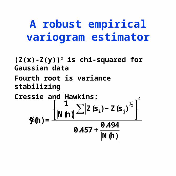
The Fourier transform

g:Rd → R

G(ω) =F (g) = g(s)exp(iωTs)ds∫

g(s) =F −1(G) =

12π( )

d exp(-iωTs)G(ω)dω∫

Properties of Fourier transforms

Convolution

Scaling

Translation

F (f∗g) =F (f)F (g)

F (f(ag)) =

1a

F(ω / a)

F (f(g−b)) =exp(ib)F (f)

Parceval’s theorem

Relates space integration to frequency integration. Decomposes variability.

f(s)2ds∫ = F(ω) 2dω∫

Aliasing

Observe field at lattice of spacing Δ. Since

the frequencies ω and ω’=ω+2πm/Δ are aliases of each other, and indistinguishable.

The highest distinguishable frequency is πΔ, the Nyquist frequency.

ΔZd

exp(iωTkΔ) = exp(i ωT+ 2π mT

Δ⎛

⎝⎜⎞

⎠⎟kΔ)

= exp(iωTkΔ)exp(i2πmTk)

Illustration of aliasing

Aliasing applet

Spectral representation

Stationary processes

Spectral process Y has stationary increments

If F has a density f, it is called the spectral density.

Z(s) = exp(isTω)dY(ω)Rd∫

E dY(ω) 2 =dF(ω)

Cov(Z(s1),Z(s2 )) = e i(s1-s2 )Tωf(ω)dωR2∫

Estimating the spectrum

For process observed on nxn grid, estimate spectrum by periodogram

Equivalent to DFT of sample covariance

In,n (ω) =1

(2πn)2z(j)eiωTj

j∈J∑

2

ω =2πj

n; J = (n − 1) / 2⎢⎣ ⎥⎦,...,n − (n − 1) / 2⎢⎣ ⎥⎦{ }

2

Properties of the periodogram

Periodogram values at Fourier frequencies (j,k)πΔ are

•uncorrelated

•asymptotically unbiased

•not consistent

To get a consistent estimate of the spectrum, smooth over nearby frequencies

Some common isotropic spectra

Squared exponential

Matérn

f(ω)=σ2

2πexp(− ω 2 / 4)

C(r) =σ2 exp(− r2 )

f(ω) =φ(2 + ω 2 )−ν−1

C(r) =πφ( r )νK ν ( r )2 ν−1Γ(ν + 1)2 ν

A simulated process

Z(s) = gjk cos 2πjs1

m+

ks2

n⎡⎣⎢

⎤⎦⎥+Ujk

⎛⎝⎜

⎞⎠⎟k=−15

15

∑j=0

15

∑

gjk =exp(− j+ 6 −ktan(20°) )

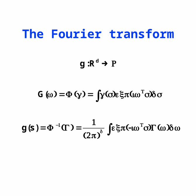
Thetford canopy heights

39-year thinned commercial plantation of Scots pine in Thetford Forest, UK

Density 1000 trees/ha

36m x 120m area surveyed for crown height

Focus on 32 x 32 subset

Spectrum of canopy heights

Whittle likelihood

Approximation to Gaussian likelihood using periodogram:

where the sum is over Fourier frequencies, avoiding 0, and f is the spectral density

Takes O(N logN) operations to calculate

instead of O(N3).

l (θ) = logf(ω;θ) +

IN,N(ω)f(ω;θ)

⎧⎨⎩

⎫⎬⎭ω

∑

Using non-gridded data

Consider

where

Then Y is stationary with spectral density

Viewing Y as a lattice process, it has spectral density

Y(x) =Δ−2 h(x−s)∫ Z(s)ds

h(x) =1( xi ≤Δ / 2, i =1,2)

fY (ω) =1Δ2 H(ω) 2

fZ(ω)

fΔ,Y (ω) = H(ω +2πqΔ

)2

fZq∈Z2∑ (ω +

2πqΔ

)

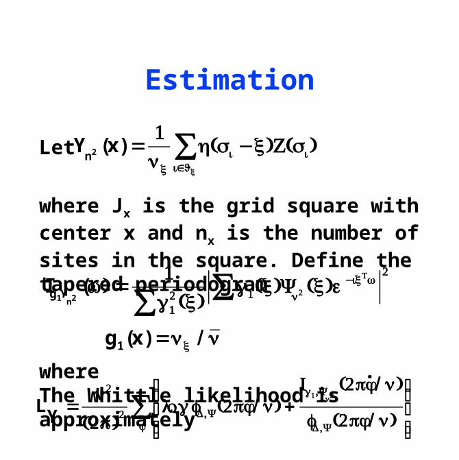
Estimation

Let

where Jx is the grid square with center x and nx is the number of sites in the square. Define the tapered periodogram

where . The Whittle likelihood is approximately

Yn2 (x) =

1nx

h(s i −x)Z(s i )i∈J x

∑

Ig1Yn2(ω) =

1g1

2 (x)∑g1(x)Yn2 (x)e−ixTω∑

2

g1(x) =nx / n

LY

=n2

2π( )2 logfΔ,Y (2πj / n) +

Ig1,Yn2(2πj / n)

fΔ,Y (2πj / n)

⎧⎨⎪

⎩⎪

⎫⎬⎪

⎭⎪j∑

A simulated example

Estimated variogram