Mechanics of Biomaterials - University of Sydney
37
The University of Sydney Slide 1 Mechanics of Biomaterials Presented by Andrian Sue AMME4981/9981 Semester 1, 2016 Lecture 7
Transcript of Mechanics of Biomaterials - University of Sydney

The University of Sydney Slide 1
Mechanics of Biomaterials
Presented byAndrian SueAMME4981/9981Semester 1, 2016
Lecture 7
The University of Sydney Slide 2
Mechanics Models

The University of Sydney Slide 3
Last Week
– Using motion to find forces and moments in the body (inverse problems)

The University of Sydney Slide 4
This Week
– Using the forces and moments to determine the stresses

The University of Sydney Slide 5
Elastic Behaviour
Hooke’s Law (Uniaxial) 𝜎 = 𝐸ϵ– Strain is directly proportional to the stress (Young’s modulus)
Hooke’s Law (General) [𝜎] = [𝑆][𝜖]– Stress tensor [𝜎]– Strain tensor [𝜖]– Stiffness tensor [𝑆]
[𝜖] = [𝑆])*[𝜎] = [𝐶][𝜎]– Compliance tensor [𝐶] = [𝑆])*
The University of Sydney Slide 6
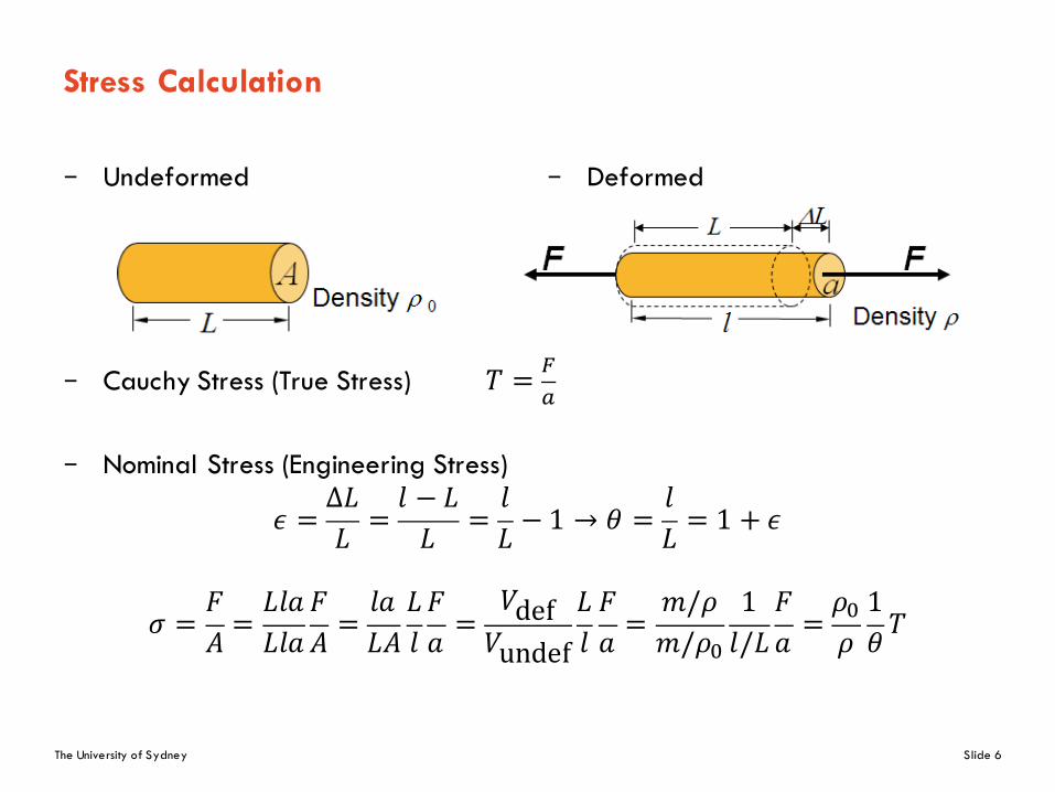
Stress Calculation
– Undeformed
– Cauchy Stress (True Stress) 𝑇 = -.
– Nominal Stress (Engineering Stress)
𝜖 =Δ𝐿𝐿 =
𝑙 − 𝐿𝐿 =
𝑙𝐿 − 1 → 𝜃 =
𝑙𝐿 = 1 + 𝜖
𝜎 =𝐹𝐴 =
𝐿𝑙𝑎𝐿𝑙𝑎
𝐹𝐴 =
𝑙𝑎𝐿𝐴
𝐿𝑙𝐹𝑎 =
𝑉def𝑉undef
𝐿𝑙𝐹𝑎 =
𝑚/𝜌𝑚/𝜌C
1𝑙/𝐿
𝐹𝑎 =
𝜌C𝜌1𝜃 𝑇
– Deformed

The University of Sydney Slide 7
Elastic Constants
Young’s Modulus, E– Relationship between tensile or compressive stress and strain– Only applies for small strains (within the elastic range)
*Assume linear, elastic, isotropic material
Biomaterial E (GPa)*Cancellous bone 0.49Cortical bone 14.7Long bone - Femur 17.2Long bone - Humerus 17.2Long bone - Radius 18.6Long bone - Tibia 18.1Vertebrae - Cervical 0.23Vertebrae - Lumbar 0.16

The University of Sydney Slide 8
Elastic Constants
Poisson’s Ratio, ν– Describes the lateral deformation in response to an axial load
𝜈 = −𝜖lateral𝜖axial
aFF
l Density ρ
L ΔL
r R

The University of Sydney Slide 9
Elastic Constants
Shear Modulus (or Lame’s second constant), G, μ– Describes the relationship between applied torque and angle of
deformation
𝐺 = 𝜇 =𝜏𝛾 =
ShearStressShearStrain
Bulk Modulus, K– Describes the resistance to uniform compression (hydrostatic pressure)
𝐾 = −Δ𝑃𝑒 = −
Δ𝑃Δ𝑉/𝑉 ≈ −𝑉
𝜕𝑃𝜕𝑉
Lame’s first constant, λ– Used to simplify the stiffness matrix in Hooke’s law

The University of Sydney Slide 10
Elastic Constants
– Young’s Modulus, E 𝐸 = X(Z[\]X)[\X = [(*\_)(*)]_)
_ = 2𝐺(1 + 𝜈)
– Poisson’s Ratio, ν 𝜈 = []([\X) =
[(Za)[) =
b]X − 1
– Shear Modulus, G, μ 𝐺 = [(*)]_)]_ = b
](*\_)
– Bulk Modulus, K 𝐾 = bZ(*)]_)
– Lame’s Constant, λ 𝜆 = ]X_*)]_ =
X(b)]X)ZX)b = b_
(*\_)(*)]_)
The University of Sydney Slide 11
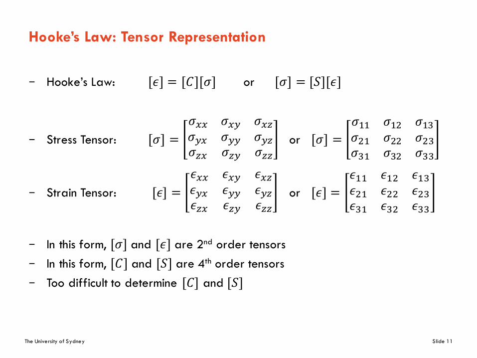
Hooke’s Law: Tensor Representation
– Hooke’s Law: [𝜖] = [𝐶][𝜎] or [𝜎] = [𝑆][𝜖]
– Stress Tensor: [𝜎] =𝜎dd 𝜎de 𝜎df𝜎ed 𝜎ee 𝜎ef𝜎fd 𝜎fe 𝜎ff
or [𝜎] =𝜎** 𝜎*] 𝜎*Z𝜎]* 𝜎]] 𝜎]Z𝜎Z* 𝜎Z] 𝜎ZZ
– Strain Tensor: [𝜖] =𝜖dd 𝜖de 𝜖df𝜖ed 𝜖ee 𝜖ef𝜖fd 𝜖fe 𝜖ff
or [𝜖] =𝜖** 𝜖*] 𝜖*Z𝜖]* 𝜖]] 𝜖]Z𝜖Z* 𝜖Z] 𝜖ZZ
– In this form, [𝜎] and [𝜖] are 2nd order tensors– In this form, [𝐶] and [𝑆] are 4th order tensors– Too difficult to determine [𝐶] and [𝑆]

The University of Sydney Slide 12
Hooke’s Law: Matrix Representation
– Hooke’s Law: {𝜖} = [𝐶]{𝜎}
𝜖 =
𝜖*𝜖]𝜖Z𝜖i𝜖j𝜖k
=
𝜖**𝜖]]𝜖ZZ2𝜖]Z2𝜖*Z2𝜖*]
[𝐶] =
𝐶** 𝐶*] 𝐶*Z𝐶]* 𝐶]] 𝐶]Z𝐶Z* 𝐶Z] 𝐶ZZ𝐶i* 𝐶i] 𝐶iZ𝐶j* 𝐶j] 𝐶jZ𝐶k* 𝐶k] 𝐶kZ
𝐶*i 𝐶*j 𝐶*k𝐶]i 𝐶]j 𝐶]k𝐶Zi 𝐶Zj 𝐶Zk𝐶ii 𝐶ij 𝐶ik𝐶ji 𝐶jj 𝐶jk𝐶kj 𝐶kj 𝐶kk
𝜎 =
𝜎*𝜎]𝜎Z𝜎i𝜎j𝜎k
=
𝜎**𝜎]]𝜎ZZ𝜎]Z𝜎*Z𝜎*]
– In this form, {𝜎} and {𝜖} are 1st order vectors– In this form, [𝐶] is a 2nd order tensor– Much easier to determine [𝐶]– This is called the Voigt notation – reduces the order of the symmetric tensor

The University of Sydney Slide 13
Constitutive Material Models
The University of Sydney Slide 14
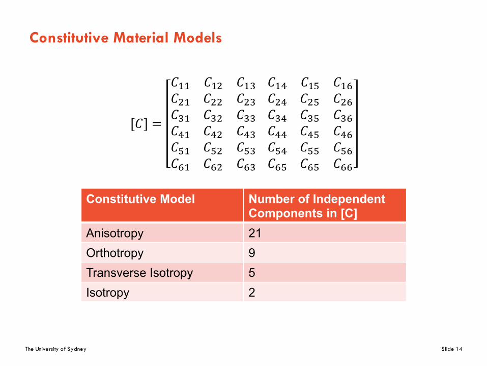
Constitutive Material Models
[𝐶] =
𝐶** 𝐶*] 𝐶*Z𝐶]* 𝐶]] 𝐶]Z𝐶Z* 𝐶Z] 𝐶ZZ𝐶i* 𝐶i] 𝐶iZ𝐶j* 𝐶j] 𝐶jZ𝐶k* 𝐶k] 𝐶kZ
𝐶*i 𝐶*j 𝐶*k𝐶]i 𝐶]j 𝐶]k𝐶Zi 𝐶Zj 𝐶Zk𝐶ii 𝐶ij 𝐶ik𝐶ji 𝐶jj 𝐶jk𝐶kj 𝐶kj 𝐶kk
Constitutive Model Number of Independent Components in [C]
Anisotropy 21Orthotropy 9Transverse Isotropy 5Isotropy 2

The University of Sydney Slide 15
Anisotropy
– Most general form of Hooke’s law– 21 independent components– Example: wood
{𝜖} = [𝐶]{𝜎}
𝜖**𝜖]]𝜖ZZ2𝜖]Z2𝜖*Z2𝜖*]
=
𝐶** 𝐶*] 𝐶*Z𝐶]* 𝐶]] 𝐶]Z𝐶Z* 𝐶Z] 𝐶ZZ𝐶i* 𝐶i] 𝐶iZ𝐶j* 𝐶j] 𝐶jZ𝐶k* 𝐶k] 𝐶kZ
𝐶*i 𝐶*j 𝐶*k𝐶]i 𝐶]j 𝐶]k𝐶Zi 𝐶Zj 𝐶Zk𝐶ii 𝐶ij 𝐶ik𝐶ji 𝐶jj 𝐶jk𝐶ki 𝐶kj 𝐶kk
𝜎**𝜎]]𝜎ZZ𝜎]Z𝜎*Z𝜎*]
– Symmetric matrix: 𝐶*] = 𝐶]*,𝐶*Z = 𝐶Z*,𝑒𝑡𝑐.
The University of Sydney Slide 16
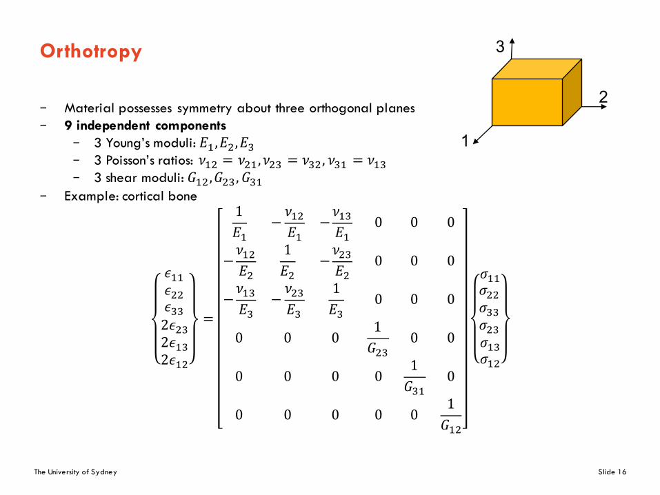
Orthotropy
– Material possesses symmetry about three orthogonal planes– 9 independent components
– 3 Young’s moduli: 𝐸*,𝐸],𝐸Z– 3 Poisson’s ratios: 𝜈*] = 𝜈]*,𝜈]Z = 𝜈Z], 𝜈Z* = 𝜈*Z– 3 shear moduli: 𝐺*],𝐺]Z, 𝐺Z*
– Example: cortical bone
𝜖**𝜖]]𝜖ZZ2𝜖]Z2𝜖*Z2𝜖*]
=
1𝐸*
−𝜈*]𝐸*
−𝜈*Z𝐸*
0 0 0
−𝜈*]𝐸]
1𝐸]
−𝜈]Z𝐸]
0 0 0
−𝜈*Z𝐸Z
−𝜈]Z𝐸Z
1𝐸Z
0 0 0
0 0 01𝐺]Z
0 0
0 0 0 01𝐺Z*
0
0 0 0 0 01𝐺*]
𝜎**𝜎]]𝜎ZZ𝜎]Z𝜎*Z𝜎*]
1
2
3
The University of Sydney Slide 17
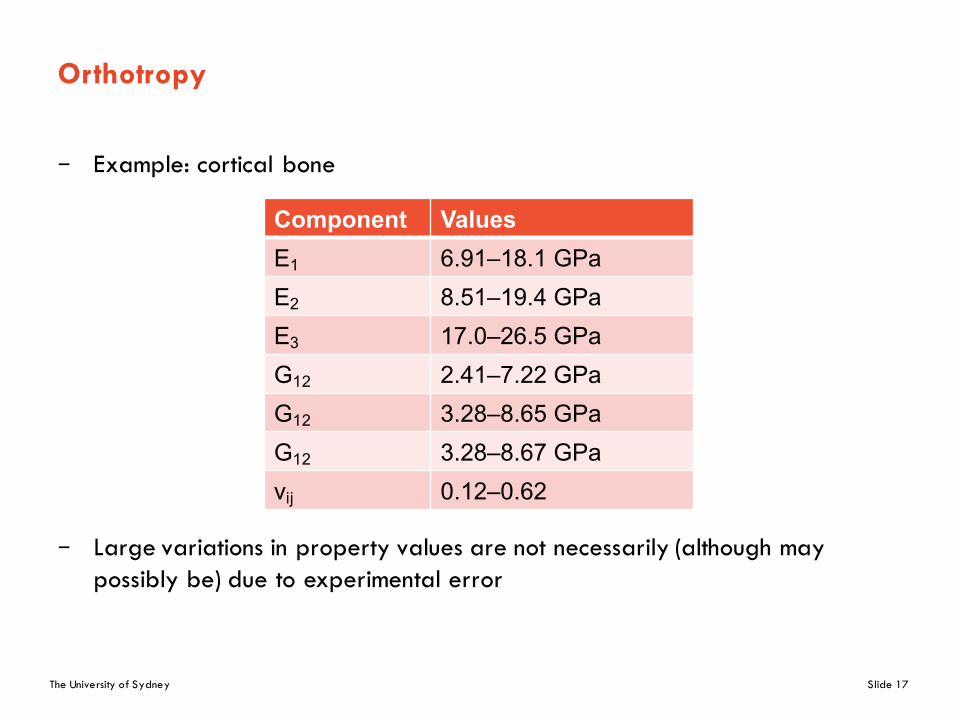
Orthotropy
– Example: cortical bone
– Large variations in property values are not necessarily (although may possibly be) due to experimental error
Component ValuesE1 6.91–18.1 GPaE2 8.51–19.4 GPaE3 17.0–26.5 GPaG12 2.41–7.22 GPaG12 3.28–8.65 GPaG12 3.28–8.67 GPaνij 0.12–0.62

The University of Sydney Slide 18
Transverse Isotropy
– 5 independent components– Young’s moduli: 𝐸* = 𝐸], 𝐸Z– Poisson’s ratios: 𝜈*] = 𝜈]*, 𝜈]Z = 𝜈Z] = 𝜈Z* = 𝜈*Z– Shear modulus: 𝐺]Z = 𝐺Z*, 𝐺*] =
bq](*\_qr)
– Example: skin
𝜖**𝜖]]𝜖ZZ2𝜖]Z2𝜖*Z2𝜖*]
=
1𝐸*
−𝜈*]𝐸*
−𝜈*Z𝐸*
0 0 0
−𝜈*]𝐸*
1𝐸*
−𝜈*Z𝐸*
0 0 0
−𝜈*Z𝐸Z
−𝜈*Z𝐸Z
1𝐸Z
0 0 0
0 0 01𝐺Z*
0 0
0 0 0 01𝐺Z*
0
0 0 0 0 02(1 + 𝜈*])
𝐸*
𝜎**𝜎]]𝜎ZZ𝜎]Z𝜎*Z𝜎*]
1
23

The University of Sydney Slide 19
Isotropy
– 2 independent components
– Young’s modulus: 𝐸 = 𝐸* = 𝐸] = 𝐸Z– Poisson’s ratio: 𝜈 = 𝜈*] = 𝜈]Z = 𝜈Z*, 𝐺 = 𝐺]Z = 𝐺Z* = 𝐺*] =
b](*\_)
– Example: Ti-6Al-4V
𝜖**𝜖]]𝜖ZZ2𝜖]Z2𝜖*Z2𝜖*]
=
1𝐸 −
𝜈𝐸 −
𝜈𝐸 0 0 0
−𝜈𝐸
1𝐸 −
𝜈𝐸 0 0 0
−𝜈𝐸 −
𝜈𝐸
1𝐸 0 0 0
0 0 02(1 + 𝜈)
𝐸 0 0
0 0 0 02(1 + 𝜈)
𝐸 0
0 0 0 0 02(1 + 𝜈)
𝐸
𝜎**𝜎]]𝜎ZZ𝜎]Z𝜎*Z𝜎*]
1
2
3

The University of Sydney Slide 20
Hooke’s Law (Isotropic): Stress-Strain Relationship
𝜎 = 𝑆 𝜖 ⇔ 𝜎tu = 𝜆𝑡𝑟 𝜖 𝛿tu + 2𝜇𝜖tu
𝑡𝑟 𝜖 = 𝜖dd + 𝜖ee + 𝜖ff 𝛿tu = x1𝑖𝑓𝑖 = 𝑗0𝑖𝑓𝑖 ≠ 𝑗
𝜎dd =b
*\_ *)]_[ 1 − 𝜈 𝜖dd + 𝜈 𝜖ee + 𝜖ff ]
𝜎ee =b
*\_ *)]_[ 1 − 𝜈 𝜖ee + 𝜈 𝜖ff + 𝜖dd ]
𝜎ff =b
*\_ *)]_[ 1 − 𝜈 𝜖ff + 𝜈 𝜖dd + 𝜖ee ]
𝜎de =b
*\_𝜖de
𝜎ef =b
*\_𝜖ef
𝜎fd =b
*\_𝜖fd
or
𝜎dd = 𝜆 𝜖dd + 𝜖ee + 𝜖ff + 2𝐺𝜖dd𝜎ee = 𝜆 𝜖dd + 𝜖ee + 𝜖ff + 2𝐺𝜖ee𝜎ff = 𝜆 𝜖dd + 𝜖ee + 𝜖ff + 2𝐺𝜖ff
𝜎de = 2𝐺𝜖de𝜎ef = 2𝐺𝜖ef𝜎fd = 2𝐺𝜖fd

The University of Sydney Slide 21
Hooke’s Law (Isotropic): Strain-Stress Relationship
𝜖 = 𝐶 𝜎 ⇔ 𝜖tu =1 + 𝜈𝐸
𝜎tu −𝜈𝐸𝑡𝑟 𝜎 𝛿tu
𝑡𝑟 𝜎 = 𝜎dd + 𝜎ee + 𝜎ff 𝛿tu = x1𝑖𝑓𝑖 = 𝑗0𝑖𝑓𝑖 ≠ 𝑗
𝜖dd =*b[𝜎dd − 𝜈 𝜎ee + 𝜎ff ]
𝜖ee =*b[𝜎ee − 𝜈 𝜎ff + 𝜎dd ]
𝜖ff =*b[𝜎ff − 𝜈 𝜎dd + 𝜎ee ]
𝜖de =*\_b
𝜎de
𝜖ef =*\_b
𝜎ef
𝜖fd =*\_b
𝜎fd
or
𝜖dd =*b[𝜎dd − 𝜈 𝜎ee + 𝜎ff ]
𝜖ee =*b[𝜎ee − 𝜈 𝜎ff + 𝜎dd ]
𝜖ff =*b[𝜎ff − 𝜈 𝜎dd + 𝜎ee ]
𝜖de =*]X𝜎de
𝜖ef =*]X𝜎ef
𝜖fd =*]X𝜎fd

The University of Sydney Slide 22
Biomechanics

The University of Sydney Slide 23
Biomechanics Methods
There are three methods that can be used to determine the biomechanical responses to loads:
1. Analytical method (Mechanics of Solids 1 and 2)
2. Biomechanical experimentation (testing)
3. Numerical techniques (FEM)

The University of Sydney Slide 24
Analytical Method: General Case
𝜖}}𝜖~~𝜖ff2𝜖~f2𝜖f}2𝜖}~
=
1𝐸}
−𝜈~}𝐸~
−𝜈f}𝐸f
0 0 0
−𝜈}~𝐸}
1𝐸~
−𝜈f~𝐸f
0 0 0
−𝜈}f𝐸}
−𝜈~f𝐸~
1𝐸f
0 0 0
0 0 01𝐺~f
0 0
0 0 0 01𝐺f}
0
0 0 0 0 01𝐺}~
𝜎}}𝜎~~𝜎ff𝜎~f𝜎f}𝜎}~
z (3)
y (2) x (1)
ez
et
en

The University of Sydney Slide 25
𝜎ff = −-��
𝜖}}𝜖~~𝜖ff2𝜖~f2𝜖f}2𝜖}~
=
1𝐸}
−𝜈~}𝐸~
−𝜈f}𝐸f
0 0 0
−𝜈}~𝐸}
1𝐸~
−𝜈f~𝐸f
0 0 0
−𝜈}f𝐸}
−𝜈~f𝐸~
1𝐸f
0 0 0
0 0 01𝐺~f
0 0
0 0 0 01𝐺f}
0
0 0 0 0 01𝐺}~
00𝜎ff000
=
−𝜈f}𝜎ff𝐸f
−𝜈f~𝜎ff𝐸f𝜎ff𝐸f000
z (3)
y (2) x (1)
ez
et
en
Fz Fz
Analytical Method: Pure Axial Load
The University of Sydney Slide 26
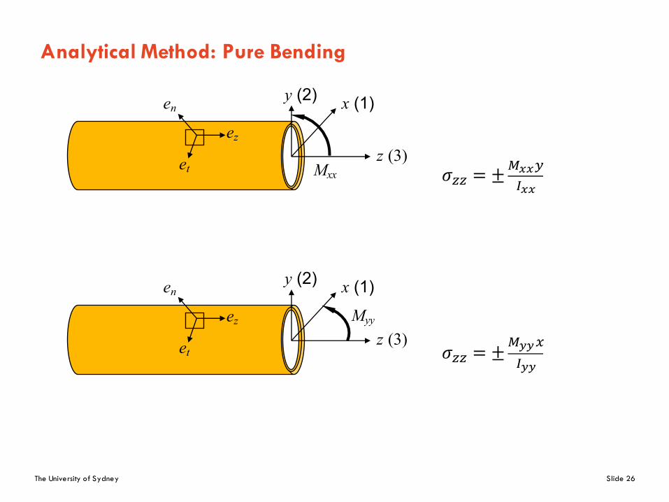
Analytical Method: Pure Bending
𝜎ff = ±���e���
𝜎ff = ±���d���
z (3)
y (2) x (1)
ez
et
en
Mxx
z (3)
y (2) x (1)
ez
et
en
Myy

The University of Sydney Slide 27
Analytical Method: Eccentric Axial Load
Using the principle of superposition
𝜎ff = −-�� ±
���e���
± ���d���
= 𝐹f −*� ±
e�e���± d�d
���
𝜎 = − -�
𝜎 = ±�e�
z (3)
y (2) x (1)
ez
et
enFz Fz ( )y~,x~
x
y

The University of Sydney Slide 28
Example: Analytical Method
Determine the maximum compressive stress on the bone, given F=200N, M=10Nm, the outer diameter of the bone is do=5cm, and the inner diameter of the bone is di=3cm.
Using the principle of superposition:
𝜎 = −�e� −
-� [𝐼 = �
i (𝑟�i − 𝑟ti), 𝐴 = 𝜋 𝑟�] − 𝑟t] ]
𝜎 = − *C×C.C]j��× C.C]j�)C.C*j� −
]CC�× C.C]jr)C.C*jr
𝜎 = −1.095𝑀𝑃𝑎
F FMM
The University of Sydney Slide 29
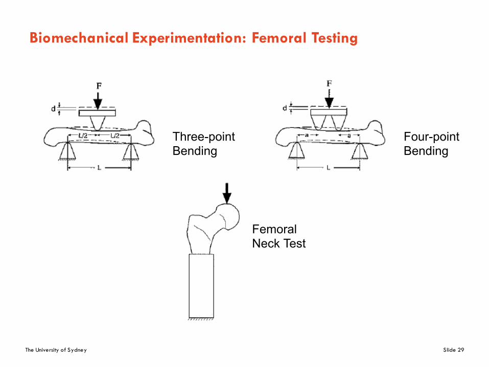
Biomechanical Experimentation: Femoral Testing
Three-pointBending
Four-pointBending
FemoralNeck Test

The University of Sydney Slide 30
Numerical Techniques: Bovine Femur Modelling
Bovine Femur Sample CT Scanning ScanIP Modelling
Angela Shi, 2010 (Thesis)

The University of Sydney Slide 31
Experimentation & Numerical Techniques: Bovine Femur
Specimen from bovine femur sample
in-vitro experimental setup
ScanCAD model
Angela Shi, 2010 (Thesis)

The University of Sydney Slide 32
Experimentation & Numerical Techniques: Bovine Femur
XFEM fracture analysis
Angela Shi, 2010 (Thesis)

The University of Sydney Slide 33
Numerical Techniques: Inhomogeneity of Bone
HU
E
pCEHU ρρ =→∝
Material relationAngela Shi, 2010 (Thesis)

The University of Sydney Slide 34
Experimentation & Numerical Techniques: Femur Fracture
– In-vitro test of cadaver model – eXtend FEM (XFEM) in Abaqus
Angela Shi, 2010 (Thesis)

The University of Sydney Slide 35
Numerical Techniques: Dental Prostheses
– Whole Jaw Model
– Partial Jaw Model
CT Image Segmentation Sectional Curves CAD Model FE Model
PDLMolar

The University of Sydney Slide 36
Numerical Techniques: Dental Prostheses
– 3 unit, all ceramic dental bridge
Solid Model Von Mises Stress

The University of Sydney Slide 37
Summary
– Mechanics models– Elastic constants
– Constitutive material models– Number of independent components required to describe the material
model– Biomechanics
– Determining the biomechanical response to loads through analytical methods, biomechanical experimentation, and numerical techniques