Meat Demand in South Korea: An Application of the...

Meat Demand in South Korea: An Application of the Restricted Source

Differentiated AIDS Model

Shida Rastegari Henneberry and Seong–huyk Hwang

The first difference version of the restricted source–differentiated almost ideal demand system is

used to estimate South Korean meat demand. The results of this study indicate that the United

States has most to gain from an increase in the size of the South Korean imported meat market in

terms of its beef exports, while South Korea has the most to gain from this expansion in the pork

market. Moreover, the results indicate that the United States has a competitive advantage to

Australia in the South Korean beef market. Results of this study have implications for U.S. meat

exports in this ever–changing policy environment.

Key words: AIDS, source differentiation, South Korean meat demand, U.S. competitiveness

JEL Classifications: D12, Q17.

The authors are professor and graduate student, respectively, in the Department of Agricultural Economics, Oklahoma State University. Senior authorship is shared. This study was partially funded by the Hatch Project No. 2537 of the Oklahoma State University Agricultural Experiment Station. The authors wish to thank three anonymous reviewers and the editor of the Journal for their useful comments and insights.

Rising per capita incomes and the rapid economic growth in South Korea during the last two

decades, has brought about a significant change towards western life styles and diets in urban

areas. This change has led to an increase in consumption of animal protein compared to the

traditional Korean staple food of cereal and vegetables. From 1980 to 2003, per capita meat

consumption (beef, pork and chicken) changed from 11.3 kg to 30.9 kg, an increase of 173%.

During the same period; self–sufficiency for beef, pork, and chicken decreased from 97.8% to

36.3%, 100% to 93.8%, and 100% to 76.7%, respectively. In 2003, South Koreans consumed the

greatest amount of pork (16.9 kg/person) followed by beef (7.9 kg/person) and chicken (6.1

kg/person), (KREI). The size of the South Korean imported meat market is expected to grow

even further in the future with expectations of continued economic growth and market–access

measures negotiated in bilateral and multilateral agreements.

The South Korean government has taken major steps in the last decade to open their borders

to foreign meat suppliers, which had led to South Korea becoming an increasingly important

player in the global markets (MAF). In 2003, South Korea was the second largest market for U.S.

beef, fourth for U.S. pork, and sixth for U.S. poultry; importing $816 million, $79 million, and

$50 million of U.S. beef, pork, and poultry meats, respectively. Understanding this emerging

market and factors shaping it, are of importance to the U.S. meat producers, marketers and policy

makers in developing effective marketing programs targeted towards expanding sales and market

shares in South Korea and in future trade negotiations.

In this light, the primary objective of this study is to estimate a meat demand system for

South Korea, differentiating meats by type and by source of origin. More specifically, the

objective of this study is to analyze the impact of economic factors on U.S. competitiveness in

the South Korean meat import market and to provide estimates of meat import demand

elasticities for this market.

Following a historical overview of the South Korean meat trade policies and review of other

studies related to Pacific Rim meat markets, a model of South Korean meat demand is specified

and the estimation results are discussed.

South Korean Meat Trade Policies and Related Studies

In the past, the South Korean government restricted the importation of meats through a quota

system, which had been in effect since 1988. Given the rapid growth of meat product markets in

Korea, major meat–exporting countries such as the United States and Australia requested an

opening of the South Korean market for beef imports through GATT and WTO negotiations.

With the establishment of the quota system, importation of beef resumed after six years of no

trade (USDA–ERS).

During 1988–2003, significant progress was made in reducing South Korean meat import

barriers. Beef quotas were raised from 123,000 tons in 1995 to 225,000 tons in 2000. The beef

market became liberalized on January 1, 2001, when a tariff–only system became effective and

the state trading of beef imports were discontinued. With regards to frozen pork and chicken,

quotas were raised from 1995 through the first half of 1997; and absolute quotas were ended on

July 1, 1997. Tariffs were lowered from 1995 levels to 25% and 20% in 2004 for frozen pork and

poultry, respectively (Dyck and Nelson). However, at the end of 2003, this liberalization

progress was interrupted when South Korea banned beef imports from the United States because

of a case of mad cow disease in the United States (USDA–ERS).

As a result of the liberalization, South Korea became the world’s ninth largest meat

importing country and the world’s fourth largest beef importing country in 2003. Furthermore,

among the Asian countries, South Korea has become the second largest imported meat market

after Japan; with imports accounting for two–thirds of volume of beef consumed in 2003 (MAF).

In particular, Korean meat imports from the United States have increased significantly during the

last several years with the U.S. share of the Korean imported meat market in terms of volume

increasing from 40% in 1993 to 53% in 2003 (KATI). As a percentage of total South Korean

meat consumption volume, imports from the United States grew from accounting for 4% in 1993

to 19% in 2003 (KATI & KREI).

The South Korean market is differentiated in terms of buyers’ attitudes towards meats

imported from various sources. The grain–fed beef imported from the United States, accounting

for 69% of volume of imports, has generally been viewed as having a higher quality than beef

imported from other sources. About 70% of imports from the United States were under the high

price category of ribs, loin, strip loin, and tenderloin; while this figure was only 29% for

Australia. Over 88% of U.S. exports and about 42% of Australian exports to South Korea were

in the form of ribs and chuck roll. It is important to recognize these quality differences in meats

when analyzing the South Korean meat import demand. Through a market research survey, Kim

et al. examined the attitude of the hotel sector beef purchasers towards the grain–fed beef

products from major potential supplying countries. Survey results indicated that the United

States has been successful in creating a positive image with the Korean international hotel sector

for grain–fed “made in the U.S.A.” brand beef, while the Canadian beef does not have the same

perceived customer value in the hotel sector. Australian beef exporters in the past have targeted

their grass–fed beef to the price–sensitive general retail sector.

Despite becoming an emerging market for U.S. meats, published research on the analysis of

South Korean meat demand is limited. Most of the previous studies addressing global demand

have focused on Japan as an important export destination for U.S. meats (Hayes, Wahl, and

Williams; Wahl and Hayes; Yang and Koo). Regarding South Korean meat demand, most of the

past studies have used aggregate consumer or wholesale–level data, without differentiating

imported meats as a separate category (Koo, Yang, and Lee; Hayes, Ahn, and Baumel; Byrne, et

al.). Jung and Koo, in their study of South Korean demand for meat and fish products,

differentiated beef into Hanwoo (beef from domestic cattle) and import quality beef. However; in

their study, imported beef was included as an aggregate category (not differentiated by supply

source) and imported pork and chicken were not included.

A Model of South Korean Meat Import Demand System

The Armington trade model and the Almost Ideal Demand System (AIDS) have been used in the

literature for the analysis of source–differentiated import demands. Although the Armington

trade model differentiates goods by countries of origin, it suffers from the restrictive assumptions

of a single constant elasticity of substitution (CES) and homotheticity, which may lead to biased

parameter estimates (Yang and Koo). As an alternative to the Armington trade model, AIDS

model has been used in import demand estimations. The AIDS model represents a flexible

complete demand system and it does not require the additivity of the utility function. It satisfies

the axioms of choice exactly and under certain conditions, aggregates perfectly over consumers

(Deaton and Muellbauer). Due to its advantages, the AIDS model has been utilized in the

analysis of both macro and micro demand systems and has been a popular tool for researchers.

Since the main objective of this study is to analyze the impact of economic variables on U.S.

competitiveness in the South Korean meat import market, a Source Differentiated AIDS

(SDAIDS) model is used. The SDAIDS is a modified version of the AIDS model, which allows

for source differentiation of various types of meats without imposing block separability. One of

the main advantages of SDAIDS includes estimates that do not suffer from aggregation bias over

import sources or over goods. The SDAIDS model is generally estimated using instrumental

variable techniques (Yang and Koo), which are expected to result in more reliable parameter

estimates.

Following Yang and Koo, the SDAIDS model is specified as:

(1) *

ln( ) lnh h h k k hi i i j j i

j k

Ew p

Pα γ β = + +

∑∑

where subscripts i and j indicate goods ( , 1,2, ,i j N= K ), and h and k indicate countries of

origin or sources. Good i may be imported from m different origins, while good j may

have n origins (where i j≠ , 1, ,h m= K , and 1, ,k n= K ). hi

w measures the budget share of good

i imported from source h (product hi ), kj

p is the price of good j imported from source k

(product kj ), E is the total expenditure on all goods in this demand system, and *P is a price

index defined as:

(2) * *

0

1ln( ) ln( ) ln( ) ln( )

2h h h k h ki i i j i j

i h i h j k

P p p pα α γ= + +∑∑ ∑∑∑∑

The SDAIDS model in (1) above is nonlinear due to the nonlinear price index in (2). To

make the system linear, Deaton and Muellbauer suggest using the Stone’s price index, here

specified as:

*ln ln( )h hi ii h

P w p=∑ ∑

However, using the above price index may create a simultaneous–equation bias ashi

w , which is

used as a dependent variable in equation (1), is employed as an independent variable in the

Stone’s price index. To avoid simultaneity, Eales and Unnevehr suggest using lagged hi

w in the

Stone’s price index.

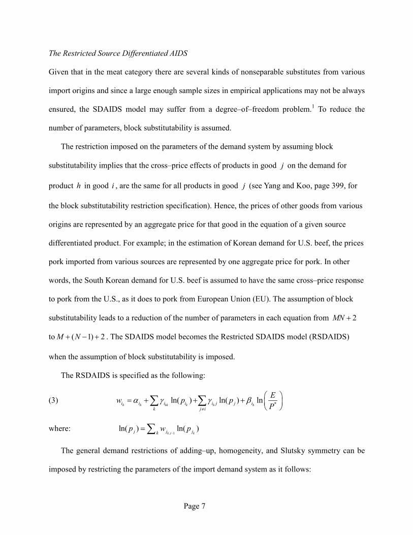
The Restricted Source Differentiated AIDS

Given that in the meat category there are several kinds of nonseparable substitutes from various

import origins and since a large enough sample sizes in empirical applications may not be always

ensured, the SDAIDS model may suffer from a degree–of–freedom problem.1 To reduce the

number of parameters, block substitutability is assumed.

The restriction imposed on the parameters of the demand system by assuming block

substitutability implies that the cross–price effects of products in good j on the demand for

product h in good i , are the same for all products in good j (see Yang and Koo, page 399, for

the block substitutability restriction specification). Hence, the prices of other goods from various

origins are represented by an aggregate price for that good in the equation of a given source

differentiated product. For example; in the estimation of Korean demand for U.S. beef, the prices

pork imported from various sources are represented by one aggregate price for pork. In other

words, the South Korean demand for U.S. beef is assumed to have the same cross–price response

to pork from the U.S., as it does to pork from European Union (EU). The assumption of block

substitutability leads to a reduction of the number of parameters in each equation from 2MN +

to ( 1) 2M N+ − + . The SDAIDS model becomes the Restricted SDAIDS model (RSDAIDS)

when the assumption of block substitutability is imposed.

The RSDAIDS is specified as the following:

(3) *

ln( ) ln( ) lnh h hk k h hi i i i i j j i

k j i

Ew p p

Pα γ γ β

≠

= + + +

∑ ∑

where: , 1

ln( ) ln( )k t kj j jk

p w p−

=∑

The general demand restrictions of adding–up, homogeneity, and Slutsky symmetry can be

imposed by restricting the parameters of the import demand system as it follows:

(4) Adding–up: 1hi

i h

α =∑∑ ; 0hki

h

γ =∑ ; 0hi j

i h

γ =∑∑ ; 0hi

i h

β =∑∑

(5) Homogeneity: 0hk hi i j

k j i

γ γ≠

+ =∑ ∑

(6) Symmetry: hk khi iγ γ=

Because of block substitutability, the symmetry conditions among goods do not apply here.

Marshallian measures of price elasticities are computed from the estimated parameters as:

(7) 1 hh

h h h

h

i

i i i

iw

γε β= − + −

(8) hk k

h k h

h h

i i

i i i

i i

w

w w

γε β

= −

(9) h

h h

h h

i j j

i j i

i i

w

w w

γε β

= −

Equation (7) represents own–price elasticities, (8) represents cross–price elasticities between the

same goods from different sources, and (9) represents cross–price elasticities between different

goods.

Expenditure elasticity is specified as:

(10) 1 h

h

h

i

i

iw

βη = +

To test for the statistical significance of price and expenditure elasticities, standard errors were

calculated using the variance of a linear transformation of the elasticity formulas (equations 7–

10). The method offered by Mdafri and Brorsen was used here to calculate the standard errors

and subsequently the statistical significance of the elasticities.2

The Empirical Model

In the empirical analysis of the demand system, the properties of homogeneity and/or symmetry

are often rejected. This is normally due to the fact that consumers are unlikely to adjust

instantaneously to changes in price, income, or other determinants of demand. Such consumers’

behavior might be caused by psychological factors, such as habit formation, habit persistence, or

due to inventory adjustments (Kesavan et al.). Likewise; institutional factors, such as changing

from an import quota system to liberalized trade, contribute to the observed lagged effects in the

analysis of import demand. Therefore, the demand behavior might be best represented by models

allowing for dynamic adjustments. To allow for lagged effects, dynamic models include lagged

dependent variables and lagged residuals as exogenous variables. However, due to the small

sample size in this study, the first difference AIDS model is used here as suggested by Ealse and

Unnevehr.3

(11) *

ln( ) ln( ) lnh hk k h hi i i i j j i

k j i

Ew p p

Pγ γ β

≠

∆ = ∆ + ∆ + ∆

∑ ∑

Data and Estimation Procedure

Quarterly data from 1996 to 2003 were used to estimate the parameters of the RSDAIDS. The

meats studied here are: pork, poultry, and other meats. Other meats include offal, mutton, lamb,

and meats of horse, rabbit, and deer. In this study, weak separability of fish and nonfish meats is

assumed, as this assumption could not be tested due to data limitations on domestic fish

consumption for the period of this study.4 However, separability of fish and nonfish meats in

South Korea has been tested and supported in the literature (Koo, Yang, and Lee; Bryne, et al.;

Capps, et al.). Nevertheless; following Hayes, Wahl, and Williams, a test of separability in the

South Korean imported meat market between fish and nonfish meats (as an aggregate group and

nonsource differentiated) was conducted. Results indicate that separability could not be rejected

at the 5% significance level.

South Korea imports meats from various sources. A country was identified as a supply source

if imports from that source constituted over 10% of the total South Korean imports of the

selected meat. Otherwise, importations are included in the Rest–of–the–World (ROW) category.

Using this criterion, the source differentiated imported meats are: beef from the United States

and Australia; pork from Canada, the U.S., and EU; and poultry from the United States and

Thailand. The other meats category is not separated by import sources.

Because retail/wholesale level prices for imported meats were not available, unit value

import prices were used to measure market prices for imported meats. Data on import value (in

thousand dollars) and quantity (in metric tons) were from KCS. Source–differentiated import

prices (unit values) for individual meats were calculated by dividing the total import value by the

total import quantity.5 Data were then converted from U.S. dollars into Won (South Korean

currency), using current exchange rates from KCS. Quantities of domestic meat consumption and

prices were reported at the wholesale level and were obtained from NACF. The summary of

sample statistics of source–differentiated expenditure shares for each meat is presented in Table 1.

[Place Table 1 Approximately Here]

In order to take into account the impact of foot and mouth disease (FMD) outbreak in 1999

and 2002; in another version of the model, a dummy variable for FMD was included as an

intercept shifter. However, this dummy variable was not statistically significant. In addition,

dummy variables reflecting seasonality in meat demand were included in the pretest estimation.

Although the variables were significant, they were not included in the final version of the model

because of the small sample size and the subsequent degrees–of–freedom problem. Instead, data

were adjusted for seasonality using the X–11 method developed by the U.S. Bureau of the

Census (SAS). The X–11 procedure provides seasonal adjustment of time series data.

Various hypotheses regarding South Korean consumer behavior were tested and applied to

the RSDAIDS model of the South Korean meat import demand system (equation 11). These

hypotheses include: product aggregation, block separability, and the endogeneity of expenditure

and prices. System misspecification is also tested.

Product Aggregation and Block Separability

The RSDAIDS model used in this study is based on the assumption that consumers place

different values on the same commodity, originating from different countries. However, this

assumption needs to be tested. Product aggregation test is used to assess whether various

products (e.g., beef supplied from various origins) could be considered as one aggregate group

(nonsource differentiation).6

Additionally, in a two–stage demand analysis, weak separability is frequently assumed as a

maintained hypothesis. Here, for parsimonious estimations, we are interested to know whether

we could study various types of meats separate from each other. The meats studied here are beef,

pork, poultry and other meats (including mutton and lamb). If separability is assumed, each type

of meat (e.g., beef) could be considered as separable from other meats (e.g., pork and poultry) at

a more aggregate level. Block separability allows for each type of meat to be estimated

individually, without having to incorporate price of other meats. In this study, the test by

Moschini, Moro, and Green is used to test for block separability. Using the following parametric

restrictions, the block separability in the RSDAIDS model is tested:

(12) ( ) ( )( )

( ) ( )( )

h h h h

h m h h

i j i j i i j j

k m k m k k m m

w w w w

w w w w

γ β β

γ β β

+ + +=

+ + +

for ( , )h hi k A∈ and ( , )j m B∈ , for all A B≠

where A and B refer to commodity groups (e.g., beef or pork) and other variables are as defined

before.

The Wald F–test was used to test the hypothesis of product aggregation over different supply

sources. This test was conducted by imposing restrictions related to the assumptions of product

aggregation (as described earlier), on the parameters of the RSDAIDS model.

Test results for block separability indicate the rejection of the null hypothesis that beef, pork,

poultry, and other meats are separable from one another at the 1% significance level (Table 2).

Therefore, the results indicate that studying each meat separate from each other is not an

appropriate assumption for the South Korean source–differentiated meat import demand

estimation. Subsequently, the null hypothesis of product aggregation was tested and was rejected

at the 1% significance level, supporting the use of a source–differentiated model. More

specifically, the results give support to studying domestically produced meats along with source–

differentiated imported meats.


Test of Endogeneity

Endogenous prices and expenditure might lead to biased and inconsistent parameter estimates. In

the model used in this study, the expenditure variable (E in equation 11) might not be truly

exogenous as expenditure is used to compute the dependent variable (Henneberry,

Piewthongngam, and Qiang; Thompson). In addition; since the import quota system was in effect

during part of the estimation period of this study, this would have meant that meat import

quantities were first set by source of origin and then prices were determined by forces of demand

and given the fixed supplies. Therefore, meat prices may be endogenous during the study period.

Moreover, long lags (exceeding one year in the case of beef) in production response to prices,

might result in relatively fixed meat supply in the short–run leading to simultaneous–equation

bias (Wahl and Hayes).

Wu–Hausman endogeneity test as described by Johnston and DiNardo (See, p.342), was

employed in this study to test for endogeneity of price and expenditure variables. This test was

performed by regressing potentially endogenous variables (prices and expenditures) on a set of

instrumental variables (auxiliary regression).7 From this regression, the residuals were calculated

and were included in the RSDAIDS as additional explanatory variables. A joint test was

conducted to see whether the coefficients of these residuals equal to zero. If these coefficients

statistically equal to zero, it can be concluded that endogeneity does not exist. From the test

results; the endogeneity of the expenditure and prices of beef from the United States, Australia,

and the ROW, and prices for pork from Canada and EU could not be rejected (Table 3).

Interestingly, test results suggest that poultry prices are uniformly exogenous. These results are

expected as the production cycle for poultry is less than one year, allowing producers to respond

to price changes within the observation period.


System Misspecification Tests

Functional form, static and dynamic homoskedasticity, and autocorrelation tests, as suggested by

McGuirk et al., are used here to test for system misspecification. Test results are presented in

Table 4. From the results of the system misspecification tests (Table 4), it can be concluded that

the null hypotheses of linearity, static and dynamic homoskedasticity, and no autocorrelation can

not be rejected at the 1% significance level. To test for parameter stability, this study employed

the single–equation Chow test and the period at the elimination of trade barriers was determined

as a dividing point for the Chow test. From the test results, the null hypothesis that variance

during the first period equals to variance during the second period cannot be rejected at the 5%

significance level. To test for normality, the Jarque–Bera test was performed. Results show that

the assumption of normality of the error terms, in each of the estimated equations, can not be

rejected at the 5% significance level.


Results

Prior to model estimation, it is necessary to test the stochastic properties of the data. Thus,

using the standard augmented Dickey–Fuller (ADF) unit root test, it was checked whether data

were stationary or nonstationary. From the results of the ADF unit root test; it was concluded that

all variables in levels were nonstationary, while all the first difference variables were stationary.8

Therefore, the results imply that given the utilized data in this study; the first difference

RSDAIDS model, as compared with the static RSDAIDS, is appropriate for estimations.

Moreover, the adjusted Wald F–test as described in Eales and Unnevehr was used to test for

homogeneity and symmetry restrictions. Results for homogeneity (across commodities) and

symmetry (for each commodity, across sources) in the first difference RSDAIDS (equation 11)

showed that these properties could not be rejected at the 5% significance level.

Because of the endogeneity of some of the prices and expenditure; the model (equation 11)

was estimated using an iterative 3SLS method of estimation, assuming block substitutability and

with homogeneity and symmetry (applied to products belonging to same category of good)

imposed. Because of the assumption of block substitutability, the symmetry condition among

goods could not be imposed.

Because meat expenditure shares (hi

w ) sum to one, the demand system composed of

expenditure share equations for the four source–differentiated meats would be singular.

Therefore, the last equation (other meats) was dropped from the system for estimation purposes.

The coefficients of the dropped equation were then calculated from the adding–up restriction.

Here, we dropped another equation and reestimated the system in order to determine the

parameters and the standard errors of the last equation. The results are the same as calculating the

parameters of the last equations from the adding–up condition.

Marshallian demand elasticities were calculated from the estimated parameters (Table 5).9 In

the beef market, all expenditure elasticities are positive and beef from Korea and the United

States have statistically significant expenditure elasticities. Beef from the South Korean domestic

cattle (Hanwoo) shows the highest expenditure elasticity (1.67), as compared to the imported

beef. This result is consistent with the general preference of South Korean consumers for

Hanwoo beef over any imported beef, because of its perceived superior quality. Among the

imported beef products, the demand for U.S. beef is more expenditure elastic (1.59) compared to

the demand for Australian beef (0.52 and nonsignificant) and beef from the ROW (0.55 and

nonsignificant); implying a higher percentage of beef would be imported from the United States

compared to Australia and the ROW, given an increase in the size of the meat market in South

Korea. This is also consistent with the South Korean consumer preferences; as in general, U.S.

grain–fed beef is preferred to the Australian grass–fed beef.

With regard to pork expenditure elasticities; all elasticities are positive, but only the elasticity

for South Korean pork is statistically significant (0.39). These results are also consistent with

South Korean consumer strong preferences for fresh domestically produced pork.10 Consistent

with what is expected from economic theory, the results of this study show negative source–

differentiated own–price elasticities for individual meats (except for the statistically

nonsignificant elasticities for pork imported from the United States, EU, the ROW, and poultry

from the ROW). Among these; own–price elasticities for South Korean domestically produced

beef, beef from Australia and the ROW, and poultry from Thailand are greater than one and

statistically significant. Inelastic and significant own–price responses were found for beef from

the U.S., pork from South Korea and Canada, and poultry from South Korea and the United

States.

Cross–price elasticities may indicate substitutability or complementary relationships among

products from various sources. The nonsignificant cross–price elasticities between Korean

produced Hanwoo beef and source–differentiated imported beef and pork imply no significant

impact on Hanwoo consumption as a result of imported beef or pork price changes. Therefore,

results confirm prior expectations that Hanwoo beef has the high–quality product image and

therefore is not expected to be a substitute for imported beef nor for pork. The Cross–price

elasticities between U.S. and Australian beef, although positive implying a substitute

relationship; are not significant. This is consistent with the fact that during a segment of the

period of this study, import quotas were in effect and therefore prices were not necessarily

determinant of the quantity of imports (as confirmed by price endogeneity test described earlier).

Regarding the pork market; the statistically significant and positive cross–price elasticity

shows that pork from the United States is a substitute for Canadian pork. This strong competition

is consistent with prior expectations as Canada and the United States both produce pork of

similar quality. The South Korean pork shows a statistically significant, although weak,

substitute relationship with pork from the United States and the ROW. As expected, Korean pork

shows a substitute relationship with beef. However, a statistically significant complementary

relationship is found between the EU pork on one hand and the United States and Canadian pork

on the other hand. The lack of competitiveness might be due to different pork products and cuts

of meat originating from North America and the EU. In the poultry market, the United States and

Thailand show a strong competitive relationship. Other cross–price elasticities are nonstatically

significant.

Among other cross–commodity relationships; Korean beef and poultry show a weak

complementary relationship, while Australian beef shows substitutability with poultry, and South

Korean and U.S. poultry show a complementary relationship with pork. In the next section, we

will look at the implications of these relationships.

Elasticities were also estimated from other estimations using other types of data on

consumption and imports, as well as prices. The model (equation 11) was estimated using retail

(instead of wholesale) level data for the domestic meat prices and quantities obtained from

NACF. The estimated elasticities were very similar in the pattern of change among supply

sources and commodities, to the elasticities reported in Table 5. Only, the elasticities were

slightly larger in absolute values. The model (equation 11) was also estimated assuming

exogenous prices and expenditures, using seemingly unrelated regression analysis. Although

some of the price and expenditure elasticities were similar to those reported in Table 5, others

were quite different in their magnitude and significance. Following Eakins and Gallagher,

another version of the dynamic AIDS model was also estimated which included the first

difference of the lagged values (two–lags) of variables in addition to the variables included in

equation 11. Although; the likelihood ratio test showed that the model was a slightly better fit for

the data, the results were not presented here due to the increase in the number of parameters

(more than double of those included in equation 11) and the significant decrease in the degrees of

freedom associated with the Eakins and Gallagher model.


Summary and Conclusions

This study estimates the impact of prices and expenditures on the South Korean quantity

demanded of source–differentiated meats, using the first difference version of the restricted

source–differentiated almost ideal demand system and assuming block substitutability. Tests of

three hypothesis regarding the behavior of South Korean meat consumers were conducted: (a)

separability of meat categories from one another (beef, pork, poultry, and other meats), (b)

nonsource differentiation (product aggregation) of individual meats, and (c) price and

expenditure endogeneity.

Results of separability tests indicate that the various studied meats are not separable from one

another. Additionally, nonsource differentiation was rejected and therefore domestically

produced meats as well as meats from various sources, were treated as different products and

demand estimation were conducted for these disaggregated products. Moreover, the endogeneity

of the price and expenditure variables were not rejected and therefore the demand system was

estimated using an iterative 3SLS method of estimation.

Results of this study shed light on South Korean consumer preferences with regard to

imported meats. This is one of the first studies which analyzes the South Korean meat demand,

differentiated by supply source. The calculated expenditure elasticities indicate that the U.S. has

the most to gain from an increase in the size of the imported meat market in terms of its beef

exports. Moreover, the results of this study show that in the South Korean beef market, the

United States has a competitive advantage compared to Australia. This is judging by the United

States’ relatively low own–price elasticity and high expenditure elasticity compared to Australia,

and considering the growth in South Korean consumers’ per capita incomes and the type of

meats that the United States exports. As was mentioned earlier; most of the U.S. exports are in

the form of high valued grain–fed beef, compared to Australia’s grass–fed lean beef. Therefore,

the growing per capita incomes in South Korea is expected to expand marketing potentials for

U.S. beef exporters in the future.

For pork, estimation results show that South Korea has the only significant expenditure

elasticity; which may reflect South Korean consumer preference for fresh domestically produced

pork. Moreover, the results indicate a competitive relationship between the United States and

Canada. In the poultry market, Thailand and the United States have the largest (in absolute value)

and statistically significant own–price elasticities compared to the competitors.

In an ever–changing policy environment, the results of this study would have implications for

the U.S. meat market share in South Korea. For example, U.S. pork producers might be

interested in knowing by how much they can increase their market share in South Korea after the

U.S. beef ban resulting from the discovery of BSE in December 2003 is lifted. A reduced beef

supply in South Korea has driven up local beef prices and has led to higher prices for domestic

pork. Judging from the cross–price elasticities; it can be concluded that the United States does

not have much to gain in terms of its pork exports from beef price increases in South Korea,

while most of the gain will be incurred by the South Korean domestic pork producers. Another

current application of this study is the implication of the recent Avian Influenza pandemics scare

which has reduced the consumption of poultry in South Korea. The competitive relationship

between poultry and Australian beef supports higher beef consumption in South Korea, and

might imply benefits to the Australian beef producers in terms of increased exports. Although all

imported pork show a competitive relationship with poultry, none are statistically significant.

Footnotes

1. For example; suppose we estimate SDAIDS model for South Korean meat import demand for

three types of meats, each imported from three sources. The SDAIDS model will include eleven

parameters (9 own–and cross–price parameters, plus intercept and expenditure coefficient), to be

estimated in each of the nine equations for each type of source–differentiated meat.

2. For calculating the standard errors of the estimated elasticities, the estimated parameters in

model (11) were first linearly transformed as the following:

(13) e Ab=

where e is the vector of estimated elasticities (ε ’s,η ’s), b is the vector of estimated RSDAIDS

model parameters (γ ’s, β ’s), and A is a matrix of constants (budget shares). Then, the variance

covariance matrix of e [VAR( e )] was calculated as:

(14) 'VAR( ) VAR( )e A b A=

where VAR(b ) is the variance covariance matrix of b.

3. Eales and Unnevehr mentioned that the first difference AIDS model is marginally inferior to a

dynamic AIDS model but the first difference AIDS model produces similar results. In this study

the first difference AIDS model was used to obtain more power due to the small sample size.

Considering that it is likely for the various meat prices to affect budget shares with different

lengths of lags, we employed Schwartz Information Criterion (SIC) in order to determine the

lengths of lags associated with various prices and expenditures. Although the results showed

varying numbers of lags; due to the small sample size and subsequent degrees of freedom

problems, we stayed with the first difference model.

4. In demand analysis, researchers often use multi–stage budgeting in order to reduce the number

of estimated parameters (Eales and Unnevehr). This study assumes two–stage budgeting of total

meat expenditure, with the first stage consisting of fish and nonfish meats. In the second stage,

the nonfish meats group is divided into beef, pork, and poultry, and other meats; each

differentiated by supply sources. The separability of South Korean meats from imported meats

was tested and separability was rejected. Therefore, South Korean produced meats were included

in the model.

5. Due to the lack of data on wholesale price for source–differentiated imported meats, unit

values (value divided by volume of imports) are used here to proxy market prices. However, unit

values might not be a perfect measure of wholesale market prices. For example; trade restrictions

(such as quotas) might not change the unit value for a meat from a particular import source, but

they might change wholesale market prices of meats due to supply restrictions.

6. The assumption of product aggregation has been used in part, in the literature to test perfect

substitutability among products. Perfect substitutability implies that the source differentiated

product prices are expected to be perfectly correlated and to react similarly to relevant price

changes (Hayes, Wahl and Williams). However, product aggregation may not necessarily imply

perfect substitutability. For details of product aggregation test refer to Yang and Koo, pp. 400–01.

7. In auxiliary regressions; the following instrumental variables were used in the estimation of

predicted values of prices and expenditures: source–differentiated lagged prices, consumer price

index, GDP, lagged real expenditure, and unit price of imported feed corn.

8. To save space, these results were not reported here.

9. Hicksian elasticities were not presented here as meats account for only a tiny fraction of

Korean consumers’ income and thus Marshallian and Hicksian elasticities are nearly identical.

10. However, Korean consumers do also have a preference for a small segment of the imported

pork (mainly from the EU) which is in the form of Sam–Gyup–Sal. This is one of the most

preferred parts of the pork belly and consists of alternating meat and fat layers and is used in

traditional Korean dishes.

References

Byrne, P.J., O.Jr. Capps, R. Tsai, and G.W. Williams. “Policy Implication of Trade Liberalization:

The Case of Meat Products in Taiwan and South Korea.” Agribusiness 11,4(1995): 297–

307.

Deaton, A., and J. Muellbauer. “An Almost Ideal Demand System.” American Economic Review

70(June 1980):312–26.

Dyck, J.H., and K.E. Nelson. Structure of the Global Markets for Meat. Agricultural Information

Bulletin No.785. Washington, DC:USDA–ERS, September 2003.

Eakins, J.M., and L.A. Gallagher. “Dynamic Almost Ideal Demand Systems: An Empirical

Analysis of Alcohol Expenditure.” Applied Economics 35(2003):1025–36.

Eales, J., and L. J. Unnevehr. “Demand for Beef and Chicken Products: Separability and

Structural Change.” American Journal of Agricultural Econmics 70(August 1988):521–

32.

Hayes, D.J., H. Ahn, and C.P. Baumel. “Meat demand in South Korea: A System Estimate and

Policy Projections.” Agribusiness 7,5(1991):433–46.

Hayes, D.J., T.I. Wahl, and G.W. Williams. “Testing Restriction on a Model of Japanese Meat

Demand.” American Journal of Agricultural Economics 72(August 1990):556–66.

Henneberry, S.R., K. Piewthongngam, and H. Qiang. “Consumer Food Safety Concerns and

Fresh Produce Consumption.” Journal of Agricultural and Resource Economics 24,1

(1999):98–113.

Johnston, J., and J. DiNardo. Econometric Methods, 4th ed. New York:McGraw Hill Book Co,

1997.

Jung, J., and W.W. Koo. “Demand for Meat and Fish Products in Korea.” Journal of Rural

Development 25(Winter 2002):133–52.

Kesavan, T., Z.A. Hassan, H.H. Jensen, and S.R. Johnson. “Dynamic and Long–run Structure in

U.S. Meat Demand.” Canadian Journal of Agricultural Economics 41(1993):139–53.

Kim, R.B.Y., J. Unterschultz, M. Veeman, and P. Jelen. “Analysis of the Korean Beef Market: A

study of Hotel Buyers’ Perspectives of Beef Imports From Three Major Sources.”

Agribusiness 13,4(1997):445–55.

Koo, W.W., S.R. Yang, and C.B. Lee. “Estimation of Demand for Meat in Korea.” Journal of

Rural Development 16(1993):205–22.

Korea Agricultural Trade Information (KATI). Statistics of Export and Import. Internet site:

http://www.kati.net/statistic/tradestat/interiorstat.jsp (Accessed October, 2004).

Korea Customs Service (KCS). Statistics of Export and Import. Internet site:

http://www.customs.go.kr/hp/cms/pc___000/stat/pcfe_000/pcfe_020/pcfe_020.html

(Accessed March, 2005).

Korea Rural Economic Institute (KREI). Food Balance Sheet in Korea. Internet site:

http://203.255.236.5:8000/kreistats/src/list_1.jsp?pclass=1 (Accessed May, 2005).

Mdafri, A., and B.W. Brorsen. “Demand for Red Meat, Poultry, and Fish in Morocco: An Almost

Ideal Demand System.” Agricultural Economics 9(1993):155–163.

McGuirk, A., P. Driscoll, J. Alwang, and H. Huang. “System Misspecification Testing and

Structural Change in the Demand for Meats.” Journal of Agricultural and Resource

Economics 20,1(1995):1–21.

Ministry of Agricultural and Forestry (MAF). Statistical Database. Internet site:

http://www.maf.go.kr/download.tdf?table=&f=/home/WebRoot/www/upload/data/2005/C

–7.pdf&fn=C–7.pdf (Accessed June, 2005).

Moschini, G., D. Moro, and R.D. Green. “Maintaining and Testing Separability in Demand

Systems.” American Jouranl of Agricultural Economics 76(February 1994):61–73.

National Agricultural Cooperative Federation (NACF). Data on price, supply and demand of

livestock products. Internet site: http://nature.nonghyup.com/jsp/live/animal/live1.jsp


Statistical Analysis System (SAS). Internet site: (Is there a text citation for this reference, please

check.)http://support.sas.com/onlinedoc/913/geDoc/en/etsug.hlp/x11_sect1.htm


Thompson, W. “Using Elasticities from an Almost Ideal Demand System? Watch Out for Group

Expenditure!” American Journal of Agricultural Economics 86(2004):1108–16.

U.S. Department of Agricultural, Economic Research Service (USDA–ERS). Briefing room:

South Korea. Internet site:

http://www.ers.usda.gov/Briefing/SouthKorea/basicinformation.htm (Accessed May,

2005).

Wahl, T.I., and D.J. Hayes. “Demand System Estimation with Upward–Sloping Supply.”

Canadian Journal of Agricultural Economics 38(1990):107–22.

Yang, S.R., and W.W. Koo. “Japanese Meat Import Demand Estimation with the Source

Differentiated AIDS Model.” Journal of Agricultural Resource Economics 19(2)

(1994):396–408.

Meat Demand in South Korea: An Application of the...

Documents

Transcript of Meat Demand in South Korea: An Application of the...