Measuring Polarization in High-Dimensional Data:Method and Application to Congressional Speech

Matthew Gentzkow, Stanford University and NBER∗

Jesse M. Shapiro, Brown University and NBER

Matt Taddy, Microsoft and Chicago Booth

May 2017

Abstract

We study trends in the partisanship of congressional speech from 1873 to 2016. We define

partisanship to be the ease with which an observer could infer a congressperson’s party from

a fixed amount of speech, and we estimate it using a structural choice model and methods

from machine learning. Our method corrects a severe finite-sample bias that we show arises

with standard estimators. The results reveal that partisanship is far greater in recent years than

in the past, and that it increased sharply in the early 1990s after remaining low and relatively

constant over the preceding century. Our method is applicable to the study of high-dimensional

choices in many domains, and we illustrate its broader utility with an application to residential

segregation.

∗E-mail: gentzkow@stanford.edu, jesse shapiro 1@brown.edu, taddy@microsoft.com. We acknowledge fundingfrom the Initiative on Global Markets and the Stigler Center at Chicago Booth, the National Science Foundation, theBrown University Population Studies and Training Center, and the Stanford Institute for Economic Policy Research(SIEPR). This work was completed in part with resources provided by the University of Chicago Research ComputingCenter. We thank Egor Abramov, Brian Knight, John Marshall, Suresh Naidu, Vincent Pons, Justin Rao, and GauravSood for their comments and suggestions. We also thank numerous seminar audiences and our many dedicated re-search assistants for their contributions to this project. The Pew Research Center, American National Election Studies,and the relevant funding agencies bear no responsibility for use of the data or for interpretations or inferences basedupon such uses.

1

1 Introduction

America’s two political parties speak different languages. Democrats talk about “estate taxes,”

“undocumented workers,” and “tax breaks for the wealthy,” while Republicans refer to “death

taxes,” “illegal aliens,” and “tax reform.” The 2010 Affordable Care Act was “comprehensive

health reform” to Democrats and a “Washington takeover of health care” to Republicans. Within

hours of the 2016 killing of 49 people in a nightclub in Orlando, Democrats were calling the

event a “mass shooting”—linking it to the broader problem of gun violence—while Republicans

were calling it an act of “radical Islamic terrorism”—linking it to concerns about national security

and immigration.1 Partisan language diffuses into media coverage (Gentzkow and Shapiro 2010;

Martin and Yurukoglu forthcoming) and other domains of public discourse (Greenstein and Zhu

2012; Jensen et al. 2012). Experiments and surveys show that partisan framing can have large

effects on public opinion (Nelson et al. 1997; Graetz and Shapiro 2006; Chong and Druckman

2007), and that language is one of the most basic determinants of group identity (Kinzler et al.

2007).

Is today’s partisan language a new phenomenon? In one sense, the answer is clearly no: one

can easily find examples of partisan terms in America’s distant past.2 Yet the magnitude of the

differences, the deliberate strategic choices that seem to underlie them, and the expanding role of

consultants, focus groups, and polls (Bai 2005; Luntz 2006; Issenberg 2012) suggest that what

we see today might represent a consequential change (Lakoff 2003). If the language of politics is

more partisan today than in the past, it could be contributing to deeper polarization and cross-party

animus, both in Congress and in the broader public.

In this paper, we apply tools from structural estimation and machine learning to study the

partisanship of language in the US Congress from 1873 to 2016. We specify a discrete-choice

model of speech in which political actors choose phrases to influence an audience. We define the

1The use of individual phrases such as “estate taxes” and “undocumented workers” is based on our analysis of con-gressional speech data below. For discussion of the Affordable Care Act, see Luntz (2009) and Democratic NationalCommittee (2016). For discussion of the Orlando shooting, see Andrews and Buchanan (2016).

2In the 1946 essay “Politics and the English Language,” George Orwell discusses the widespread use of politicaleuphemisms (Orwell 1946). Northerners referred to the American Civil War as the “War of the Rebellion” or the“Great Rebellion,” while southerners called it the “War for Southern Independence” or, in later years, the “War ofNorthern Aggression” (McCardell 2004). The bulk of the land occupied by Israel during the Six-Day War in 1967 iscommonly called the “West Bank,” but some groups within Israel prefer the name “Judea and Samaria,” which evokeshistorical and Biblical connections (Newman 1985). The rebels fighting the Sandinista government in Nicaragua werecommonly called “Contras,” but were referred to as “freedom fighters” by Ronald Reagan and Republican politicianswho supported them (Peace 2010).

2

overall partisanship of speech in a given period to be the ease with which an observer could guess

a speaker’s party based solely on the speaker’s choice of words. We estimate the model using the

text of speeches from the United States Congressional Record.

To compute an accurate estimate of partisanship, we must grapple with two methodological

challenges. First, natural plug-in estimators of our model suffer from severe finite-sample bias.

The bias arises because the number of phrases a speaker could choose is large relative to the total

amount of speech we observe, meaning that many phrases are said mostly by one party or the

other purely by chance. Second, although our discrete-choice model takes a standard multinomial

logit form, the large number of choices and parameters makes standard approaches to estimation

computationally infeasible. We address these challenges, respectively, by using an L1 or lasso-type

penalty on key model parameters to control bias, and a Poisson approximation to the multinomial

logit likelihood to permit distributed computing. We also suggest two tools for model-free inspec-

tion of the data: a permutation test to assess the magnitude of small-sample bias, and a leave-out

estimator for partisanship.

The methods we develop here can be applied to a broad class of problems in which the goal

is to characterize the polarization or segregation of choices in high-dimensional data. Examples

include measuring residential segregation across small geographies, polarization of web browsing

or social media behavior, and between-group differences in consumption. Whenever the number

of possible choices is large relative to the number of actual choices observed, naive estimates will

tend to suffer from finite-sample bias similar to the one we document for speech, and our penalized

estimator can provide an accurate and computationally feasible solution.

We find that the partisanship of language has exploded in recent decades, reaching an unprece-

dented level. From 1873 to the early 1990s, partisanship was relatively constant and fairly small

in magnitude: in the 43rd session of Congress (1873-75), the probability of correctly guessing a

speaker’s party based on a one-minute speech was 54 percent; by the 101st session (1989-1990)

this figure had increased to 57 percent. Beginning with the congressional election of 1994, parti-

sanship turned sharply upward, with the probability of guessing correctly based on a one-minute

speech climbing to 73 percent by the 110th session (2007-09). Methods that do not correct for

finite-sample bias—including both the maximum likelihood estimator of our model and estimates

previously published by Jensen et al. (2012)—imply instead that partisanship is no higher today

than in the past.

We unpack the recent increase in partisanship along a number of dimensions. The most partisan

3

phrases in each period—defined as those phrases most diagnostic of the speaker’s party—align well

with the issues emphasized in party platforms and, in recent years, include well-known partisan

phrases like those mentioned above. Manually classifying phrases into substantive topics shows

that the increase in partisanship is due more to changes in the language used to discuss a given topic

(e.g., “estate tax” vs. “death tax”) than to changes in the topics parties emphasize (e.g., Republicans

focusing more on taxes and Democrats focusing more on labor issues). The topics that show the

sharpest increase in recent years include taxes, immigration, crime, and religion. Separating out

phrases that first appear in the vocabulary after 1980, we find that such “neologisms” exhibit a

particularly dramatic rise in partisanship, though they are not the main driver of the overall rise

in partisanship. Comparing our measure to a standard measure of polarization based on roll-call

votes, we find that the two are correlated in the cross section but exhibit very different dynamics

in the time series. We see this as evidence that partisan language is not merely another measure of

a single latent dimension of ideological polarization, but a distinct phenomenon that has evolved

independently.

While we cannot say definitively why partisanship of language increased when it did, the evi-

dence points to innovation in political persuasion as a proximate cause. The 1994 inflection point

in our series coincides precisely with the Republican takeover of Congress led by Newt Gingrich,

under a platform called the Contract with America (Gingrich and Armey 1994). This election is

widely considered a watershed moment in political marketing, as consultants such as Frank Luntz

applied novel focus group technologies to identify effective language and disseminate it broadly to

candidates (Lakoff 2004; Luntz 2004; Bai 2005). Consistent with this, we show that phrases from

the text of the Contract with America see a spike in usage in 1994, and then exhibit a particularly

strong upward trend in partisanship. As a related factor, the years leading up to this inflection

point had seen important changes in the media environment: the introduction of television cameras

as a permanent presence in the chamber, the live broadcast of proceedings on the C-SPAN cable

channels, and the emergence of the twenty-four hour cable news cycle. Prior work suggests that

these media changes strengthened the incentive to engineer language and impose party discipline

on floor speeches (Frantzich and Sullivan 1996).

To illustrate the broader utility of our methods, the final section presents an application to

partisan residential segregation. The extent to which such polarization has been increasing is a

point of contention in the literature, with Bishop (2008) famously arguing that there has been a

“big sort” of American voters into politically homogeneous enclaves, and Glaeser and Ward (2006)

4

and Abrams and Fiorina (2012) among others arguing that this is a myth. We show that standard

segregation measures applied to this problem are severely distorted by the same finite-sample bias

that we highlight in our main application. Applying our methods to correct for this bias reveals

that the level of segregation is much lower than naive measures would suggest, and that it has not

increased significantly over time.

Our analysis relates most closely to recent work by Jensen et al. (2012). They use text from

the Congressional Record to characterize party differences in language from the late nineteenth

century to the present. Their index, which is based on the observed correlation of phrases with

party labels, implies that partisanship has been rising recently but was even higher in the past.

We apply a new method that addresses finite-sample bias and leads to substantially different con-

clusions. Lauderdale and Herzog (2016) specify a generative hierarchical model of floor debates

and estimate the model on speech data from the Irish Dail and the US Senate. They study trends

in polarization in the US Senate from 1995 to 2014 and find that polarization in speech has in-

creased faster over that period than polarization in roll-call voting. Peterson and Spirling (2016)

study trends in the polarization of speech in the UK House of Commons. In contrast to Lauderdale

and Herzog’s (2016) analysis (and ours), Peterson and Spirling (2016) do not specify a generative

model of speech. Instead, Peterson and Spirling (2016) measure polarization using the predictive

accuracy of several machine-learning algorithms. They cite our article to justify using random-

ization tests to check for spurious trends in their measure. These tests show that their measure

implies significant and time-varying polarization even in fictitious data in which speech patterns

are independent of party.

Our segregation results relate to the broader literature on residential segregation, which is sur-

veyed in Reardon and Firebaugh (2002). The finite-sample bias we highlight has been noted in

that context by Cortese et al. (1976) and Carrington and Troske (1997). Recent work has derived

axiomatic foundations for segregation measures (Echenique and Fryer 2007; Frankel and Volij

2011), asking which measures of segregation satisfy certain intuitive properties.3 Our approach

is, instead, to specify a generative model of the data and to measure segregation using objects that

have a well-defined meaning in the context of the model.4 To our knowledge, ours is among the

first papers to estimate group differences based on preference parameters in a structural model.5

3See also Mele (2013) and Ballester and Vorsatz (2014). Our measure is also related to measures of cohesiveness inpreferences of social groups, as in Alcalde-Unzu and Vorsatz (2013).

4In this respect, our paper builds on Ellison and Glaeser (1997), who use a model-based approach to measure agglom-eration spillovers in US manufacturing.

5Davis et al. (2016) use a structural demand model to estimate racial segregation in restaurant choices in a sample

5

We know of no other attempt to use a penalization scheme to address the finite-sample bias arising

in segregation measurement, which has previously been addressed by benchmarking against ran-

dom allocation (Carrington and Troske 1997), applying asymptotic or bootstrap bias corrections

(Allen et al. 2015), and estimating mixture models (Rathelot 2012, D’Haultfœuille and Rathelot

2017).6

Substantively, our findings speak to a broader literature on trends in political polarization. A

large body of work builds on the ideal point model of Poole and Rosenthal (1985) to analyze

polarization in congressional roll-call votes, finding that inter-party differences fell from the late

nineteenth to the mid-twentieth century, and have increased steadily since (McCarty et al. 2015).

We show that the dynamics of polarization in language are very different, suggesting that language

is a distinct dimension of party differentiation.7

The next sections introduce our data, model, and approach to estimation. We then present

our main estimates, along with evidence that unpacks the recent increase in partisanship. In the

following section, we discuss possible explanations for this change. In a final section, we present

results on the residential segregation of voters. We conclude by considering the wider implications

of increasing partisanship and discussing other applications of our method.

2 Congressional Speech Data

Our primary data source is the text of the United States Congressional Record (hereafter, the

Record) from the 43rd Congress to the 114th Congress. We obtain digital text from HeinOnline,

who performed optical character recognition (OCR) on scanned print volumes. The Record is

a “substantially verbatim” record of speech on the floor of Congress (Amer 1993). We exclude

of New York City Yelp reviewers. Mele (forthcoming) shows how to estimate preferences in a random-graph modelof network formation and measures the degree of homophily in preferences. Bayer et al. (2002) use an equilibriummodel of a housing market to study the effect of changes in preferences on patterns of residential segregation. Fossett(2011) uses an agent-based model to study the effect of agent preferences on the degree of segregation.

6Within the literature on measuring document partisanship (e.g., Laver et al. 2003; Gentzkow and Shapiro 2010; Kimet al. forthcoming), our approach is closest to that of Taddy (2013), but unlike Taddy (2013), we allow for a rich setof covariates and we target faithful estimation of partisanship rather than classification performance. More broadly,our paper relates to work in statistics on authorship determination (Mosteller and Wallace 1963), work in economicsthat uses text to measure the sentiment of a document (e.g., Antweiler and Frank 2004; Tetlock 2007), and work thatclassifies documents according to similarity of text (Blei and Lafferty 2007; Grimmer 2010).

7A related literature considers polarization among American voters, with most measures offering little support for thewidespread view that voters are more polarized today than in the past (Fiorina et al. 2005; Glaeser and Ward 2006;Fiorina and Abrams 2008). An exception is measures of inter-party dislike or distrust, which do show a sharp increasein recent years (Iyengar et al. 2012).

6

Extensions of Remarks, which are used to print unspoken additions by members of the House that

are not germane to the day’s proceedings.8

The modern Record is issued in a daily edition, printed at the end of each day that Congress is

in session, and in a bound edition that collects the content for an entire Congress. These editions

differ in formatting and in some minor elements of content (Amer 1993). Our data contains bound

editions for the 43rd to 111th Congresses, and daily editions for the 97th to 114th Congresses.

We use the bound edition in the sessions where it is available and the daily edition thereafter. The

Online Appendix shows that the two editions give qualitatively similar results in the years in which

they overlap.

We use an automated script to parse the raw text into individual speeches. Beginnings of

speeches are demarcated in the Record by speaker names, usually in all caps (e.g., “Mr. ALLEN

of Illinois.”). We determine the identity of each speaker using a combination of manual and au-

tomated procedures, and append data on the state, chamber, and gender of each member from

historical sources.9 We exclude any speaker who is not a Republican or a Democrat, speakers who

are identified by office rather than name, non-voting delegates, and speakers whose identities we

cannot determine.10 The results of a manual audit of the reliability of our parsing are presented in

the Online Appendix and indicate good accuracy.

The input to our main analysis is a matrix Ct whose rows correspond to speakers and whose

8The Record seeks to capture speech as it was intended to have been said (Amer 1993). Speakers are allowed to insertnew remarks, extend their remarks on a specific topic, and remove errors from their own remarks before the Recordis printed. The rules for such insertions and edits, as well as the way they appear in print, differ between the Houseand Senate, and have changed to some degree over time (Amer 1993; Johnson 1997; Haas 2015). We are not awareof any significant changes that align with the changing partisanship we observe in our data. We present our resultsseparately for the House and Senate in the Online Appendix.

9Our main source for congresspeople is the congress-legislators GitHub repositoryhttps://github.com/unitedstates/congress-legislators/tree/1473ea983d5538c25f5d315626445ab038d8141b accessedon November 15, 2016. We make manual corrections, and add additional information from ICPSR and McKibbin(1997), the Voteview Roll Call Data (Carroll et al. 2015a,b), and the King (1995) election returns. Both the publicdomain and Voteview datasets include metadata from Martis (1989).

10In the rare case in which a speaker switches parties during a term, we assign the new party to all the speechin that term. We handle the similarly rare case in which a speaker switches chambers in a single ses-sion (usually from the House to the Senate) by treating the text from each chamber as a distinct speaker-session. If a speaker begins a session in the House as a non-voting delegate of a territory and receives vot-ing privileges after the territory gains statehood, we treat the speaker as a voting delegate for the entiretyof that speaker-session. If a non-voting delegate of the House later becomes a senator, we treat each po-sition as a separate speaker-session. We obtain data on the acquisition of statehood from http://www.thirty-thousand.org/pages/QHA-02.htm (accessed on January 18, 2017) and data on the initial delegates for eachstate from https://web.archive.org/web/20060601025644/http://www.gpoaccess.gov/serialset/cdocuments/hd108-222/index.html. When we assign a majority party in each session, we count the handful of independents that caucuswith the Republicans or Democrats as contributing to the party’s majority in the Senate. Due to path dependence inour data build, such independents are omitted when computing the majority party in the House.

7

columns correspond to distinct two-word phrases or bigrams (hereafter, simply “phrases”). An

element ci jt thus gives the number of times speaker i has spoken phrase j in session (Congress)

t. To create these counts, we first perform the following pre-processing steps: (i) delete hyphens

and apostrophes; (ii) replace all other punctuation with spaces; (iii) remove non-spoken paren-

thetical insertions; (iv) drop a list of extremely common words;11 and (v) reduce words to their

stems according to the Porter2 stemming algorithm (Porter 2009).12 We then drop phrases that are

likely to be procedural or have low semantic meaning according to criteria we define in the Online

Appendix. Finally, we restrict attention to phrases spoken at least 10 times in at least one session,

spoken in at least 10 unique speaker-sessions, and spoken at least 100 times across all sessions.

The Online Appendix presents results from a sample in which we tighten each of these restrictions

by 10 percent.

The resulting vocabulary contains 508,352 unique phrases spoken a total of 287 million times

by 7,732 unique speakers. We analyze data at the level of the speaker-session, of which there are

36,161. The Online Appendix reports additional summary statistics for our estimation sample and

the phrases used to construct it.

We manually classify a subset of phrases into 22 non-mutually exclusive topics as follows.

We begin with a set of partisan phrases which we group into 22 topics (e.g., taxes, defense, etc.).

For each topic, we create a set of keywords consisting of relevant words contained in one of the

categorized phrases, plus a set of additional manually included words. Finally, we identify all

phrases in the vocabulary that include one of the topic keywords, are used more frequently than

a topic-specific occurrence threshold, and are not obvious false matches. The Online Appendix

lists, for each topic, the keywords, the occurrence threshold, and a random sample of included and

excluded phrases.

3 Model and Measure of Partisanship

3.1 Probability Model

Let cit be the J-vector of phrase counts for speaker i in session t, with mit = ∑ j ci jt denoting the

total amount of speech by speaker i in session t. Let P(i) ∈ {R,D} denote the party affiliation of

11The set of these “stopwords” we drop is defined by a list obtained fromhttp://snowball.tartarus.org/algorithms/english/stop.txt on November 11, 2010.

12Gentzkow et al. (2017) provide more intuition on the decision to represent raw text as phrase counts and on thepre-processing steps, both of which are standard in the text analysis literature.

8

speaker i, and let Rt = {i : P(i) = R,mit > 0} and Dt = {i : P(i) = D,mit > 0} denote the set of

Republicans and Democrats, respectively, active in session t. Let xit be a K-vector of (possibly

time-varying) speaker characteristics.

We assume that:

cit ∼MN(

mit ,qP(i)t (xit)

), (1)

where qPt (xit) ∈ (0,1)J for all P, i, and t. The speech-generating process is fully characterized by

the verbosity mit and the probability qPt (·) of speaking each phrase.

3.2 Choice Model

As a microfoundation for (1), suppose that at the end of session t speaker i receives a payoff:

uit =

δyt +(1−δ )(

ααα′t +x′itγγγ t

)cit , i ∈ Rt

−δyt +(1−δ )(

ααα′t +x′itγγγ t

)cit , i ∈ Dt

(2)

where

yt = ϕϕϕ′t ∑

icit (3)

is an index of public opinion that can be affected by political rhetoric. Here, ϕϕϕ t is a J-vector

mapping speech into public opinion, δ is a scalar denoting the relative importance of public opinion

in a speaker’s utility, ααα t is a J-vector denoting the baseline popularity of each phrase at time t, and

γγγ t is a K× J matrix mapping speaker characteristics into the utility of using each phrase.

Each speaker chooses each phrase she speaks to maximize uit up to a choice-specific i.i.d. type

1 extreme value shock, so that:

qP(i)jt (xit) = eui jt/∑

leuilt (4)

ui jt = δ (2 ·1i∈Rt −1)ϕ jt +(1−δ )(

α jt +x′itγγγ jt

).

Note that if xit is a constant (xit := xt), any interior phrase probabilities qPt (·) are consistent

with equation (4). In this sense, the choice model in this subsection only restricts the model in

(1) by pinning down how phrase probabilities depend on speaker characteristics. Note also that,

according to equation (4), if a phrase (or set of phrases) is excluded from the choice set, the relative

frequencies of the remaining phrases are unchanged. We exploit this fact in Sections 5 and 6 to

9

compute average partisanship for interesting subsets of the full vocabulary.

3.3 Measure of Partisanship

For given characteristics x, we think of the degree of partisanship as the divergence between qRt (x)

and qDt (x). When these vectors are close, Republicans and Democrats speak similarly and we say

that partisanship is low. When they are far from each other, languages diverge and we say that

partisanship is high.

We choose a particular measure of this divergence that has a clear interpretation in the context

of our model: the posterior probability that an observer with a neutral prior expects to assign to a

speaker’s true party after hearing the speaker speak a single phrase.

Definition. The partisanship of speech at x is:

πt (x) =12

qRt (x) ·ρρρ t (x)+

12

qDt (x) · (1−ρρρ t (x)) , (5)

where

ρ jt (x) =qR

jt (x)qR

jt (x)+qDjt (x)

. (6)

Average partisanship in session t is:

πt =1

|Rt ∪Dt | ∑i∈Rt∪Dt

πt (xit) . (7)

To understand these definitions, note that ρ jt (x) is the posterior belief that an observer with a

neutral prior assigns to a speaker being Republican if the speaker chooses phrase j in session t and

has characteristics x. Partisanship πt (x) averages ρ jt (x) over the possible parties and phrases: if

the speaker is a Republican (which occurs with probability 12 ), the probability of a given phrase j

is qRjt (x) and the probability assigned to the true party after hearing j is ρ jt (x); if the speaker is

a Democrat, these probabilities are qDjt (x) and 1−ρ jt (x), respectively. Average partisanship πt ,

which is our target for estimation, averages πt (xit) over the characteristics xit of speakers active in

session t.

10

3.4 Discussion

We frame our model in terms of our application to partisan speech. Both the model and the ap-

proaches we develop to estimation, however, are applicable to any multinomial choice problem

where we wish to characterize the divergence in choices between two groups. In Section 7 below,

we illustrate with an application to residential segregation of political parties, where i indexes US

adults rather than speakers, and the choices j are residential locations rather than phrases.

Our notion of partisanship is closely related to isolation, a common measure of residential

segregation (White 1986; Cutler et al. 1999). To see this, let mit = 1 for all i and t, so that each adult

chooses one and only one residential location. Isolation is the difference in the share Republican of

the average Republican’s location and the average Democrat’s location. In an infinite population

with an equal share of Republicans and Democrats, all with characteristics x, this is:

Isolationt (x) = qRt (x) ·ρρρ t (x)−qD

t (x) ·ρρρ t (x) (8)

= 2πt (x)−1.

Thus, isolation is an affine transformation of partisanship.

Frankel and Volij (2011) characterize a large set of segregation indices based on a set of ordinal

axioms. Ignoring covariates x, our measure satisfies six of these axioms: Non-triviality, Continuity,

Scale Invariance, Symmetry, Composition Invariance, and the School Division Property. It fails to

satisfy one axiom: Independence.13

4 Estimation

4.1 Plug-in Estimators

Ignoring covariates x, a straightforward way to estimate partisanship is to plug in empirical ana-

logues for the terms that appear in equation (5). This approach yields the maximum likelihood

estimator (MLE) of our model.

More precisely, let q̂it = cit/mit be the empirical phrase frequencies for speaker i. Let q̂Pt =

∑i∈Pt cit/∑i∈Pt mit be the empirical phrase frequencies for party P, and let ρ̂ jt = q̂Rjt/(

q̂Rjt + q̂D

jt

),

13In our context, Independence would require that the ranking in terms of partisanship of two years t and s remainsunchanged if we add a new set of phrases J∗ to the vocabulary whose probabilities are the same in both years(qP

jt = qPjs∀P, j ∈ J∗). Frankel and Volij (2011) list one other axiom, the Group Division Property, which is only

applicable for indices where the number of groups (i.e., parties in our case) is allowed to vary.

11

excluding from the choice set any phrases that are not spoken in session t. Then the MLE of πt

when xit := xt is:

π̂MLEt =

12(q̂R

t)· ρ̂ρρ t +

12(q̂D

t)· (1− ρ̂ρρ t) . (9)

Standard results imply that this estimator is consistent and efficient in the limit as the amount of

speech grows large, holding fixed the set of phrases in the vocabulary.

The MLE can, however, be severely biased in finite samples. As π̂MLEt is a convex function of

q̂Rt and q̂D

t , Jensen’s inequality implies that it has a positive bias. To build intuition for the form of

the bias, use the fact that E(q̂R

t , q̂Dt)=(qR

t ,qDt)

to decompose the bias of a generic term(q̂R

t)· ρ̂ρρ t

as:

E((

q̂Rt)· ρ̂ρρ t−

(qR

t)·ρρρ t)=(qR

t)·E(ρ̂ρρ t−ρρρ t)+Cov

((q̂R

t −qRt),(ρ̂ρρ t−ρρρ t)

). (10)

The first term is nonzero because ρ̂ρρ t is a nonlinear transformation of(q̂R

t , q̂Dt).14 Far more impor-

tant in practice, however, is that the second term is nonzero because the sampling error in ρ̂ρρ t is

mechanically related to the sampling error in(q̂R

t , q̂Dt). Intuitively, as the asymptotic properties of

the MLE require that we observe a large number of occurrences of each phrase, the bias will tend

to be greatest whenever the number of phrases (i.e., the dimensionality of the choice set) is large

relative to the total amount of speech.

A similar bias arises for plug-in estimators of polarization measures other than partisanship,

because sampling variability means that q̂Rt and q̂D

t will tend to differ by more than qRt and qD

t .

This is especially transparent if we use a norm such as Euclidean distance as a metric: Jensen’s

inequality implies that for any norm ‖·‖, E∥∥q̂R

t − q̂Dt∥∥ > ∥∥qR

t −qDt∥∥. Similar issues arise for the

measure of Jensen et al. (2012), which is given by 1mt

∑ j m jt∣∣corr

(ci jt ,1i∈Rt

)∣∣. If speech is in-

dependent of party (qRt = qD

t ), then the population value of corr(ci jt ,1i∈Rt

), conditional on total

verbosity mi, is zero. But in any finite sample the correlation will be nonzero with positive prob-

ability, so the measure may imply some amount of polarization even when speech is unrelated to

party.

One appealing approach to addressing finite-sample bias in π̂MLEt is to use different samples

to estimate q̂Pt and ρ̂ρρ t , making the errors in the former orthogonal to the errors in the latter and so

14Suppose that there are two speakers, one Democrat and one Republican, each with mit = 1. There are two phrases.The Republican says the second phrase with certainty and the Democrat says the second phrase with probability0.01. Then E(ρ̂2t) = 0.01( 1

2 )+0.99(1) = 0.995 > ρ2t = 1/1.01≈ 0.990.

12

eliminating the second bias term in equation (10). This leads naturally to a leave-out estimator:

π̂LOt =

12

1|Rt | ∑i∈Rt

q̂i,t · ρ̂ρρ−i,t +12

1|Dt | ∑

i∈Dt

q̂i,t ·(1− ρ̂ρρ−i,t

), (11)

where ρ̂ρρ−i,t is the analogue of ρ̂ρρ t computed from the empirical frequencies q̂P−i,t of all speakers

other than i.15 This estimator is consistent in the limit as the amount of speech grows, fixing the

number of phrases. It is still biased for πt (because ρ̂ρρ−i,t is biased for ρρρ t), but we show below that

the bias appears small in practice.

4.2 Penalized Estimator

Our preferred estimation method draws on the structure of the choice model in Section 3.2, allow-

ing us to include speaker characteristics xit and to control bias through penalization. Rewrite ui jt

as:16

ui jt = α̃ jt +x′it γ̃γγ jt + ϕ̃ jt1i∈Rt . (12)

The α̃ jt are phrase-time-specific intercepts and the ϕ̃ jt are phrase-time-specific party loadings. In

our baseline specification, xit consists of indicators for state, chamber, gender, Census region, and

whether the party is in the majority for the entirety of the session. The coefficients γ̃γγ jt on these

attributes are static in time (i.e., γ̃ jtk := γ̃ jk) except for those on Census region, which are allowed

to vary freely across sessions. We also explore specifications in which xit includes unobserved

speaker-level preference shocks.

We estimate the parameters {α̃αα t , γ̃γγ t , ϕ̃ϕϕ t}Tt=1 of equation (12) by minimization of the following

penalized objective function:

∑j

{∑t

∑i

[mit exp(α̃ jt +x′it γ̃γγ jt + ϕ̃ jt1i∈Rt )− ci jt(α̃ jt +x′it γ̃γγ jt + ϕ̃ jt1i∈Rt )+

ψ

(∣∣α̃ jt∣∣+∥∥∥γ̃γγ jt

∥∥∥1

)+λ j

∣∣ϕ̃ jt∣∣]}. (13)

We form an estimate π̂∗t of πt by substituting estimated parameters into the probability objects in

equation (7).

15Implicitly, in each session t we exclude any phrase that is spoken only by a single speaker.16This parameterization is observationally equivalent to equation (4), with ϕ̃ jt = 2δϕ jt , γ̃γγ jt = γγγ jt (1−δ ), and α̃ jt =(1−δ )α jt −δϕ jt .

13

The minimand in (13) encodes two key decisions. First, we approximate the likelihood of

our multinomial logit model with the likelihood of a Poisson model (Palmgren 1981; Baker 1994;

Taddy 2015), where ci jt ∼ Pois(exp[µit +ui jt

]), and we use the plug-in estimate µ̂it = logmit

of µit . Because the Poisson and the multinomial logit share the same conditional likelihood

Pr(cit | mit), their MLEs coincide when µ̂it is the MLE. Although our plug-in is not the MLE,

Taddy (2015) shows that our approach often performs well in related settings. In the Online Ap-

pendix, we show that our estimator performs well on data simulated from the multinomial logit

model.

We adopt the Poisson approximation because, fixing µ̂it , the likelihood of the Poisson is sep-

arable across phrases. This feature allows us to use distributed computing to estimate the model

parameters (Taddy 2015). Without the Poisson approximation, computation of our estimator would

be infeasible due to the cost of repeatedly calculating the denominator of the logit choice proba-

bilities.

The second key decision is the use of an L1 penalty λ j∣∣ϕ̃ jt∣∣, which imposes sparsity on the

party loadings and shrinks them toward 0 (Tibshirani 1996). We determine the penalties λλλ by reg-

ularization path estimation, first finding λ 1j large enough so that ϕ̃ jt is estimated to be 0, and then

incrementally decreasing λ 2j , ...,λ

Gj and updating parameter estimates accordingly. An attractive

computational property of this approach is that the coefficient estimates change smoothly along

the path of penalties, so each segment’s solution acts as a hot-start for the next segment and the

optimizations are fast to solve. We then choose the value of λ j that minimizes a Bayesian Infor-

mation Criterion.17 The Online Appendix reports a qualitatively similar result when we use 5-fold

cross-validation to select the λ j that minimizes average out-of-sample deviance.

We also impose a minimal penalty of ψ = 10−5 on the phrase-specific intercepts α̃ jt and the

covariate coefficients γ̃γγ jt . We do this to handle the fact that some combinations of data and covari-

ate design do not have an MLE in the Poisson model (Haberman 1973, Silva and Tenreyro 2010).

A small penalty allows us to achieve numerical convergence while still treating the covariates in a

flexible way.18

17The Bayesian Information Criterion we use is ∑i,t logPois(ci jt ; exp[µ̂i +ui jt ])+d f logn, where n = ∑t (|Dt |+ |Rt |)is the number of speaker-sessions and d f is a degrees-of-freedom term that (following Zou et al. 2007) is given bythe number of parameters estimated with nonzero values (excluding the µ̂it , as outlined in Taddy 2015).

18The Online Appendix shows how our results vary with alternative values of ψ . Larger values of ψ decrease com-putational time for a given problem. Note that in practice we implement our regularization path computationally asψλ̃ 2

j , ...,ψλ̃ Gj where λ̃ G

j = ιλ̃ 1j , ι = 10−5, and G = 100. To ensure that the choice of λ̃ j is not constrained by the

regularization path, we recommend that users choose values of ψ and ι small enough that forcing λ̃ j = λ̃ Gj for all j

14

If the penalty shrinks quickly enough with the amount of speech then, for fixed vocabulary, our

estimator behaves asymptotically like the MLE and is root-n consistent. However, as we will see,

our estimator is far less biased than the MLE. Moreover, for fixed penalty λλλ , our estimator can be

interpreted as the unique posterior mode of a Bayesian model with a diffuse Laplace prior on the

coefficients γ̃γγ , an informative Laplace prior on the party loadings ϕ̃ϕϕ , and an uninformative prior

on the intercepts α̃αα . Our parameter estimates are thus optimal for this prior against a “0-1” loss

function (Murphy 2012).

For all of our main results, we perform inference via subsampling (Politis et al. 1999). We

partition the data into 10 random subsets and re-estimate on each subset. We then report confidence

intervals based on the distribution of the estimator across these subsets, under the assumption of

root-n convergence.19 We center these confidence intervals around the estimated series and report

uncentered bias-corrected confidence intervals for our main estimator in the Online Appendix.

The Online Appendix also reports confidence intervals based on a parametric bootstrap. We do not

report results for a nonparametric bootstrap; the standard nonparametric bootstrap is known to be

invalid for lasso regression (Chatterjee and Lahiri 2011).

5 Results

5.1 Trends in Partisanship

We now turn to our main results on trends in the partisanship of speech over time. As a diagnostic

for finite-sample bias, we present, for each measure, a placebo series where we reassign parties

to speakers at random and then re-estimate the measure on the resulting data. In this “random”

series, qRt = qD

t by construction, so the true value of πt is equal to 12 in all years. We thus expect

the random series for an unbiased estimator of πt to have value 12 in each session t, and we can

measure the bias of an estimator by its deviation from 12 .

Figure 1 presents results for the maximum likelihood estimator π̂MLEt of our model, and the

index reported by Jensen et al. (2012) computed using their publicly available data.20 Panel A

shows that the random series for π̂MLE is far from 12 , indicating that the bias in the MLE is severe

either leads to π̂∗t ≈ π̂MLEt or to an estimator π̂∗t that substantially differs from the one chosen by BIC.

19The Online Appendix shows that confidence intervals based on five subsamples have similar width to those basedon ten subsamples, suggesting that our assumed learning rate is a reasonable approximation over the relevant range.

20Downloaded from http://www.brookings.edu/∼/media/Projects/BPEA/Fall-2012/Jensen-Data.zip?la=en on March25, 2016.

15

in practice. Variation over time in the magnitude of the bias dominates the series, leading the

random series and the real series to be highly correlated. Taking the MLE at face value, we would

conclude that language was much more partisan in the past and that the upward trend in recent

years is small by historical standards.

Because bias is a finite-sample property, it is natural to expect that the severity of the bias in

π̂MLEt in a given session t depends on the amount of speech, i.e., on the verbosity mt of speakers in

that session. The Online Appendix shows that this is indeed the case: a first-order approximation

to the bias in π̂MLEt as a function of verbosity follows a similar path to the random series in Panel

A of Figure 1, and the dynamics of π̂MLEt are similar to those in the real series when we allow

verbosity to follow its empirical distribution but fix phrase frequencies(qR

t ,qDt)

at those observed

in a particular session t∗. The Online Appendix also shows that while the severity of the bias falls

as we exclude less frequently spoken phrases, very severe sample restrictions are needed to control

bias, and there remains a significant time-varying bias even when we exclude 99 percent of phrases

from our calculations.

Panel B of Figure 1 shows that the Jensen et al. (2012) measure behaves similarly to the MLE.

The plot for the real series replicates the published version. The random series is again far from 12 ,

and the real and random series both trend downward in the first part of the sample period. Jensen et

al. (2012) conclude that polarization has been increasing recently, but that it was as high or higher

in earlier years. The results in Panel B suggest that the second part of this conclusion could be an

artifact of the finite-sample mechanics of their index.21

Figure 2 shows the leave-out estimator π̂LOt . The random series suggests that the leave-out

correction largely purges the estimator of bias: the series is close to 12 throughout the period. The

real series suggests that partisanship is roughly constant for much of the sample period, then rises

rapidly beginning in the 1990s.

Figure 3 presents our main result: the time series of partisanship from our preferred penalized

estimator described in Section 4.2. Panel A shows the full series, and Panel B zooms in on the most

recent years, indicating some events of interest. These estimates have two important advantages

relative to π̂LOt : they control for observables xit , and they use penalization to control bias and

reduce variance. The results show that this approach reduces both the bias and the amount of noise

in the series. The Online Appendix shows that the use of regularization is the key to this increased

21In the Online Appendix, we show that the dynamics of π̂MLEt in Jensen et al.’s (2012) data are similar to those in our

own data, which is reassuring as Jensen et al. (2012) obtain the Congressional Record independently, use differentprocessing algorithms, and use a vocabulary of three-word phrases rather than two-word phrases.

16

performance: imposing only a minimal penalty (i.e., set λλλ ≈ 0) leads to behavior qualitatively

similar to that of the MLE. The Online Appendix also shows that, in contrast to the MLE, the

dynamics of our preferred penalized estimator cannot be explained by changes in verbosity over

time.

Looking at the data through the sharper lens of our preferred estimator reveals that partisan-

ship was low and relatively constant until the early 1990s, then exploded, reaching unprecedented

heights in recent years. The plot also shows that the recent change in partisanship in our preferred

estimates is statistically significant based on our subsampling confidence intervals.

The Online Appendix presents a range of alternative series based on variants of our baseline

target, model, estimator, and sample. Targeting average Euclidian distance or average mutual infor-

mation shows a large rise in partisanship following the 1990s, though the Euclidean distance series

is noisier than our baseline measure. Removing covariates leads to greater estimated partisan-

ship while adding more controls or speaker random effects leads to lower estimated partisanship,

though all of these variants imply a large rise in partisanship following the 1990s. Dropping the

South from the sample does not meaningfully change the estimates, nor does excluding data from

early decades.

The recent increase in partisanship implied by our baseline estimates is large. Recall that

average partisanship is the posterior that a neutral observer expects to assign to a speaker’s true

party after hearing a single phrase. Figure 4 extends this concept to show the expected posterior

for speeches of various lengths. An average one-minute speech in our data contains around 33

phrases (after pre-processing). In 1874, an observer hearing such a speech would expect to have a

posterior of around 0.54 on the speaker’s true party, only slightly above the prior of 0.5. By 1990,

this value increased slightly to 0.57. Between 1990 and 2008, however, it leaped up to 0.73.

In Figure 5, we compare our speech-based measure of partisanship to the standard measure

of ideological polarization based on roll-call votes (Carroll et al. 2015a). The latter is based on

an ideal-point model that places both speakers and legislation in a latent space; polarization is

the distance between the average Republican and the average Democrat along the first dimension.

Panel A shows that the dynamics of these two series are very different: though both indicate

a large increase in recent years, the roll-call series is about as high in the late nineteenth and

early twentieth century as it is today, and its current upward trend begins around 1950 rather than

1990. We conclude from this that speech and roll-call votes should not be seen as two different

manifestations of a single underlying ideological dimension. Rather, speech appears to respond to

17

a distinct set of incentives and constraints.

Panel B of Figure 5 shows that a measure of the Republican-ness of an individual’s speech from

our model and the individual Common Space DW-NOMINATE scores from the roll-call voting

data are nevertheless strongly correlated in the cross section. Across all sessions, the correlation

between speech and roll-call based partisanship measures is 0.537 (p = 0.000). After controlling

for party, the correlation is 0.129 and remains highly statistically significant (p = 0.000).22 Thus,

members who vote more conservatively also use more conservative language on average, even

though the time-series dynamics of voting and speech diverge. As another way to validate this

relationship, we show in the Online Appendix that average partisanship exhibits a discontinuity

in vote margin analogous to the discontinuity in vote margin of the non-Common-Space DW-

NOMINATE scores (Lee et al. 2004; Carroll et al. 2015b). The Online Appendix also shows

that the divergence in speech between parties in recent years is not matched by an equally large

divergence in speech between the more moderate and more extreme wings within each party.

5.2 Partisan Phrases

Our model provides a natural way to define the partisanship of an individual phrase. For an ob-

server with a neutral prior, the expected posterior that a speaker with characteristics xit is Repub-

lican is 12 = q̄t (xit) ·ρρρ t (xit), where q̄t (·) = 1

2qRt (·)+ 1

2qDt (·) . Suppose that, unbeknownst to the

observer, phrase j is removed from the vocabulary, and the marginal probabilities of the remaining

phrases k 6= j are rescaled to q̄kt(xit)1−q̄ jt(xit)

. This corresponds to an experiment where anytime phrase j

would have been chosen, both the speaker’s party and the phrase are redrawn.23 Then the change

in the expected posterior isq̄ jt (xit)

1− q̄ jt (xit)

(ρ jt (xit)−

12

).

We define the partisanship ζ jt of phrase j in session t to be the average of this value across all

active speakers i in session t. This measure has both direction and magnitude: positive numbers

are Republican phrases, negative numbers are Democratic phrases, and the absolute value gives

the magnitude of partisanship.

Table 1 lists the ten most partisan phrases in every tenth session plus the most recent session.

22These correlations are 0.685 (p = 0.000) and 0.212 (p = 0.000), respectively, when we use data only on speakerswho speak an average of at least 1000 phrases across the sessions in which they speak.

23We also implement an alternative measure of phrase partisanship where anytime phrase j would have been chosen,the phrase but not the speaker’s party is redrawn. We compute this alternative measure for sessions 50, 70, 90, and110. The lists of the 10 most partisan phrases in each of these sessions are unchanged.

18

The Online Appendix shows the list for all sessions. These lists illustrate the underlying variation

driving our measure, and give a sense of how partisan speech has changed over time. In the Online

Appendix, we argue in detail that the top phrases in each of these sessions align closely with

the policy positions and narrative strategies of the parties, confirming that our measure is indeed

picking up partisanship rather than some other dimension that happens to be correlated with it. In

this section, we highlight a few illustrative examples.

The 50th session of Congress (1887-88) occurred in a period where the cleavages of the Civil

War and Reconstruction Era were still fresh. Republican phrases like “union soldier” and “con-

feder soldier” relate to the ongoing debate over provision for veterans, echoing the 1888 Republi-

can platform’s commitment to show “[the] gratitude of the Nation to the defenders of the Union.”

The Republican phrase “color men” reflects the ongoing importance of racial issues. Many Demo-

cratic phrases from this Congress (“increase duti,” “ad valorem,” “high protect,” “tariff tax,” “high

tariff”) reflect a debate over reductions in trade barriers. The 1888 Democratic platform endorses

tariff reduction in its first sentence, whereas the Republican platform says Republicans are “un-

compromisingly in favor of the American system of protection.”

The 80th session (1947-1948) convened in the wake of the Second World War. Many Republican-

leaning phrases relate to the war and national defense (“arm forc,” “air forc,” “coast guard,” “stop

communism,” “foreign countri”), whereas “unit nation” is the only foreign-policy-related phrase

in the top ten Democratic phrases in the 80th session. The 1948 Democratic Party platform ad-

vocates amending the Fair Labor Standards Act to raise the minimum wage from 40 to 75 cents

an hour (“labor standard,” “standard act,” “depart labor,” “collect bargain,” “concili servic”).24 By

contrast, the Republican platform of the same year does not mention the Fair Labor Standards Act

or the minimum wage.

Language in the 110th session (2007-2008) follows partisan divides familiar to modern readers.

Republicans focus on taxes (“tax increas,” “rais tax,” “tax rate”) and immigration (“illeg immigr”),

while Democrats focus on the aftermath of the war in Iraq (“war iraq”, “troop iraq”) and social

domestic policy (“african american,” “children health,” and “middl class”). With regards to energy

policy, Republicans focus on the potential of American energy (“natural gas,” “american energi,”

“outer continent,” “continent shelf”), while Democrats focus on the role of oil companies (“oil

compani”).

24The Federal Mediation and Conciliation Service was created in 1947 and was “given the mission of preventingor minimizing the impact of labor-management disputes on the free flow of commerce by providing mediation,conciliation and voluntary arbitration” (see https://www.fmcs.gov/aboutus/our-history/ accessed on April 15, 2017).

19

The phrases from the 114th session (2015-2016) relate to current partisan cleavages and echo

themes in the 2016 presidential election. Republicans focus on terrorism, discussing “al qaeda” and

using the phrase “radic islam,” which echoes Donald Trump’s use of the phrase “radical Islamic

terrorism” during the campaign (Holley 2017). They also refer repeatedly to the “american peopl.”

Democrats focus on climate change (“climat chang”), civil rights issues (“african american,” “vote

right”), and gun control (“gun violenc”). When discussing public health, Republicans focus on

mental health (“mental health”) in correspondence to the Republican-sponsored “Helping Familes

in Mental Health Crisis Act of 2016,” while Democrats focus on public health more broadly (“pub-

lic health”), health insurance (“afford care”), and women’s health (“plan parenthood”).

5.3 Partisanship within and between Topics

Our baseline measure of partisanship captures changes both in the topics speakers choose to discuss

and in the phrases they use to discuss them. Whether a speech about taxes includes the phrases

“tax relief” or “tax breaks” will help an observer to guess the speaker’s party; so, too, will whether

the speaker chooses to talk about taxes or about the environment. To separate these, we present a

decomposition of partisanship into within- and between-topic components using our 22 manually

defined topics.

We define between-topic partisanship to be the expected posterior that a neutral observer ex-

pects to assign to a speaker’s true party when the observer knows only the topic a speaker chooses,

not the particular phrases chosen within the topic. Partisanship within a specific topic is the ex-

pected posterior when the vocabulary consists only of phrases in that topic. The overall within-

topic partisanship in a given session is the average of partisanship across all topics, weighting each

topic by its frequency of occurrence.

Figure 6 shows that the rise in partisanship is driven mainly by divergence in how the parties

talk about a given substantive topic, rather than by divergence in which topics they talk about.

According to our estimates, choice of topic encodes much less information about a speaker’s party

than does choice of phrases within a topic.

Figure 7 shows estimated partisanship for phrases within each of the 22 topics. Partisanship

has increased within many topics in recent years, with the largest increases in the immigration,

crime, and religion topics. Other topics with large increases include taxes, environmental policy,

and minorities. Not all topics have increased recently however. Alcohol, for example, was fairly

partisan in the Prohibition Era but is not especially partisan today. Figure 7 also shows that the

20

partisanship of a topic is not strongly related in general to the frequency with which the topic is

discussed. For example, the world wars are associated with a surge in the frequency of discussion

of defense, but not with an increase in the partisanship of that topic.

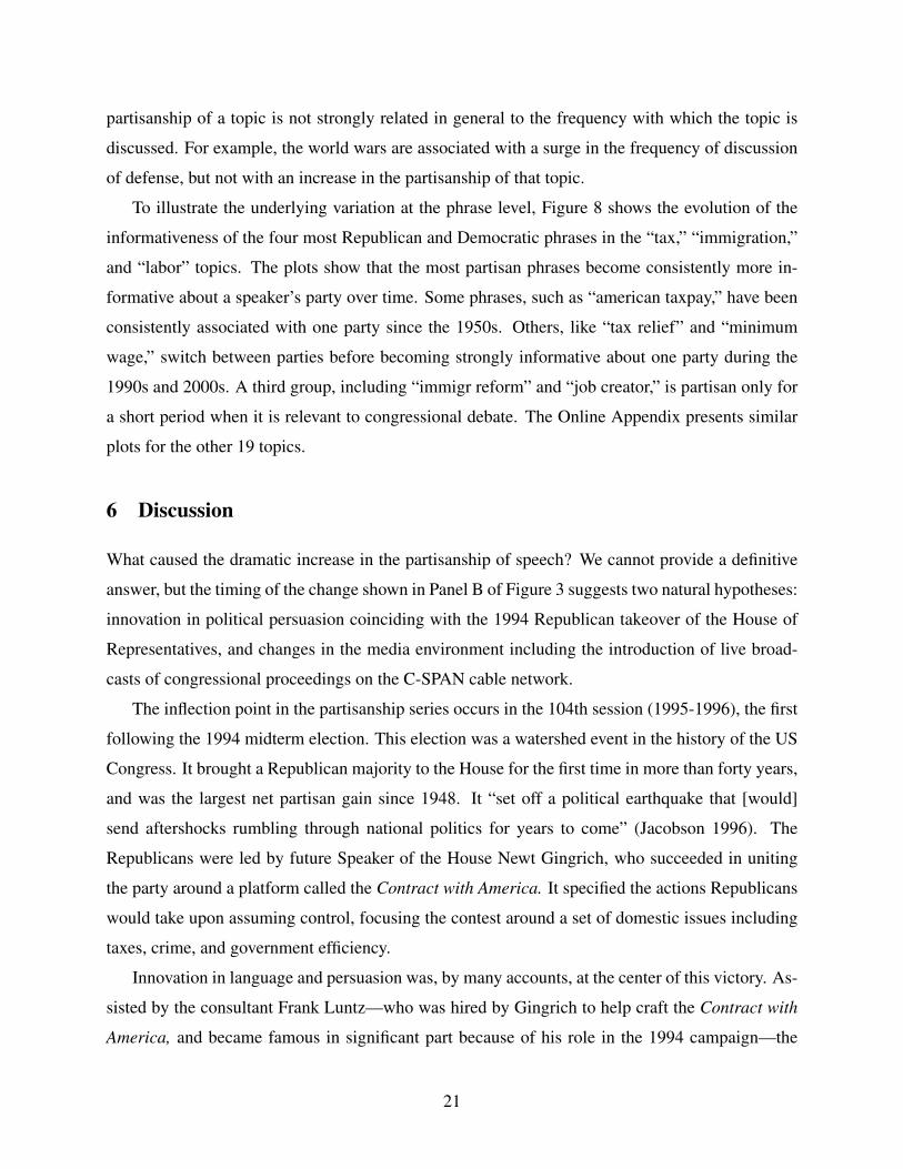
To illustrate the underlying variation at the phrase level, Figure 8 shows the evolution of the

informativeness of the four most Republican and Democratic phrases in the “tax,” “immigration,”

and “labor” topics. The plots show that the most partisan phrases become consistently more in-

formative about a speaker’s party over time. Some phrases, such as “american taxpay,” have been

consistently associated with one party since the 1950s. Others, like “tax relief” and “minimum

wage,” switch between parties before becoming strongly informative about one party during the

1990s and 2000s. A third group, including “immigr reform” and “job creator,” is partisan only for

a short period when it is relevant to congressional debate. The Online Appendix presents similar

plots for the other 19 topics.

6 Discussion

What caused the dramatic increase in the partisanship of speech? We cannot provide a definitive

answer, but the timing of the change shown in Panel B of Figure 3 suggests two natural hypotheses:

innovation in political persuasion coinciding with the 1994 Republican takeover of the House of

Representatives, and changes in the media environment including the introduction of live broad-

casts of congressional proceedings on the C-SPAN cable network.

The inflection point in the partisanship series occurs in the 104th session (1995-1996), the first

following the 1994 midterm election. This election was a watershed event in the history of the US

Congress. It brought a Republican majority to the House for the first time in more than forty years,

and was the largest net partisan gain since 1948. It “set off a political earthquake that [would]

send aftershocks rumbling through national politics for years to come” (Jacobson 1996). The

Republicans were led by future Speaker of the House Newt Gingrich, who succeeded in uniting

the party around a platform called the Contract with America. It specified the actions Republicans

would take upon assuming control, focusing the contest around a set of domestic issues including

taxes, crime, and government efficiency.

Innovation in language and persuasion was, by many accounts, at the center of this victory. As-

sisted by the consultant Frank Luntz—who was hired by Gingrich to help craft the Contract with

America, and became famous in significant part because of his role in the 1994 campaign—the

21

Republicans used focus groups and polling to identify rhetoric that resonated with voters (Bai

2005).25 Important technological advances included the use of instant feedback “dials” that al-

lowed focus group participants to respond to the content they were hearing in real time.26 Asked

in an interview whether “language can change a paradigm,” Luntz replied:

I don’t believe it—I know it. I’ve seen it with my own eyes.... I watched in 1994 when

the group of Republicans got together and said: “We’re going to do this completely

differently than it’s ever been done before....” Every politician and every political party

issues a platform, but only these people signed a contract (Luntz 2004).

A 2006 memorandum written by Luntz and distributed to Republican congressional candidates

provides detailed advice on the language to use on topics including taxes, budgets, social security,

and trade (Luntz 2006).

We can use our data to look directly at the importance of the Contract with America in shaping

congressional speech. We extract all phrases that appear in the text of the Contract and treat them

as a single “topic,” computing both their frequency and their partisanship in each session. Figure

9 reports the results. As expected, the frequency of these phrases spikes in the 104th session

(1995-1996). Their partisanship rises sharply in that year and continues to increase even as their

frequency declines.27

In the years after 1994, Democrats sought to replicate what they perceived to have been a

highly successful Republican strategy. George Lakoff, a linguist who advised many Democratic

candidates, writes: “Republican framing superiority had played a major role in their takeover of

Congress in 1994. I and others had hoped that... a widespread understanding of how framing

worked would allow Democrats to reverse the trend” (Lakoff 2014).

The new attention to crafting language coincided with attempts to impose greater party dis-

cipline in speech. In the 101st session (1989-1991), the Democrats established the “Democratic

Message Board” which would “defin[e] a cohesive national Democratic perspective” (quoted from

25By his own description, Luntz specializes in “testing language and finding words that will help his clients... turnpublic opinion on an issue or a candidate” (Luntz 2004). A memo called “Language: A Key Mechanism of Control”circulated in 1994 to Republican candidates under a cover letter from Gingrich stating that the memo contained“tested language from a recent series of focus groups” (GOPAC 1994).

26Luntz said, “[The dial technology is] like an X-ray that gets inside [the subject’s] head... it picks out every singleword, every single phrase [that the subject hears], and you know what works and what doesn’t” (Luntz 2004).

27According to the metric defined in Table 1, the most Republican phrases in the 104th session (1995-1996) thatappear in the Contract are “american peopl,” “tax increas,” “term limit,” “lineitem veto,” “tax relief,” “save ac-count,” “creat job,” “tax credit,” “wast fraud,” and “fiscal respons.” We accessed the text of the Contract athttp://wps.prenhall.com/wps/media/objects/434/445252/DocumentsLibrary/docs/contract.htm on May 18, 2016.

22

party documents in Harris 2013). The “Republican Theme Team” formed in the 102nd session

(1991-1993) sought likewise to “develop ideas and phrases to be used by all Republicans” (Michel

1993 and quoted in Harris 2013).

Consistent with this trend towards greater party discipline, Figure 10 shows that the recent

increase in partisanship is concentrated in a small minority of highly partisan phrases. The figure

plots quantiles of the estimated average value of the partisanship of all individual phrases in each

session. The plot shows a marked increase in the partisanship of the highest quantiles, while even

the quantiles at 0.9 and 0.99 remain relatively flat.

In a similar vein, Figure 11 shows that a vocabulary consisting of neologisms—which we define

to be phrases first spoken in our data after 1980 (the 96th session)—exhibits very high and sharply

rising partisanship. The figure also shows that a large increase in partisanship remains even when

we exclude neologisms from the choice set.28

Changes in the media environment may also have contributed to the increase in partisanship.29

Prior to the late 1970s, television cameras were only allowed on the floor of Congress for special

hearings and events. With the introduction of the C-SPAN cable network to the House in 1979,

and the C-SPAN2 cable network to the Senate in 1986, every speech was recorded and broadcast

live. While live viewership of these networks has always been limited, they created a video record

of speeches that could be used for subsequent press coverage and in candidates’ advertising. This

plausibly increased the return to carefully crafted language, both by widening the reach of success-

ful sound bites, and by dialing up the cost of careless mistakes.30 The subsequent introduction of

the Fox News cable network and the increasing partisanship of cable news more generally (Martin

and Yurukoglu forthcoming) may have further increased this return.

The timing shown in Figure 3 is inconsistent with the C-SPAN networks being the proximate

cause of increased partisanship. But it seems likely that they provided an important complement

to linguistic innovation in the 1990s. Gingrich particularly encouraged the use of “special order”

speeches outside of the usual legislative debate protocol, which allowed congresspeople to speak

directly for the benefit of the television cameras. The importance of television in this period is

underscored by Frantzich and Sullivan (1996): “When asked whether he would be the Republican

leader without C-SPAN, Ginigrich... [replied] ‘No’... C-SPAN provided a group of media-savvy28The Online Appendix shows that results are very similar when we instead define a neologism to be a phrase such

that at least 99 percent of its occurrences are after 1980 (the 96th session).29Our discussion of C-SPAN is based on Frantzich and Sullivan (1996).30Mixon et al. (2001) and Mixon et al. (2003) provide evidence that the introduction of C-SPAN changed the nature

of legislative debate.

23

House conservatives in the mid-1980s with a method of... winning a prime-time audience.”

7 Extension: Residential Segregation of Voters

In this section, we apply our method to generate new measures of the segregation of US voters

by party. Trends in political segregation have been a major point of contention in the literature,

with Bishop (2008) among others arguing that there has been a “big sort” of American voters into

politically homogeneous enclaves, while Glaeser and Ward (2006) and Abrams and Fiorina (2012)

among others argue that such increasing segregation is a myth. A key stumbling block has been

that existing analysis is based on voting patterns, which confound changes in the distribution of

voters with changes in the positions of candidates: a pattern of more districts voting exclusively

Republican or exclusively Democratic could be produced by either sorting of voters or increasing

extremity of candidates. Abrams and Fiorina (2012) argue that the appropriate measure should use

individuals’ party identification rather than their votes, and should consider sub-county-level data.

To our knowledge, no such analysis has yet been conducted, presumably in part because there is

no large-sample data on self-reported party affiliation by small geographies.

Our method allows us to get around this limitation because we can produce valid estimates us-

ing smaller samples from survey data. We combine county-level data from the American National

Election Studies (ANES 2015) and Pew Research Center (Pew 2016) to examine segregation in

party identification between 1956 and 2009, and zipcode-level data on political contributions from

the Federal Election Commission (FEC 2015) to examine sub-county segregation in contributions

between 1980 and 2015. The Online Appendix provides details on data sources and construction.

To apply our model, we let i index individuals and j index locations. We assume that each

individual makes a single choice, so that mit = 1 for all i, and the outcome ci jt is an indicator equal

to one if person i lives in location j in year t. Party P(i) ∈ {R,D} is either i’s self-described party

affiliation or the party to which they contribute. Partisanship is then defined as above, and can be

interpreted as the expected posterior a neutral observer would assign to an individual’s true party

after observing where they choose to live. We present both the MLE and our preferred penalized

estimator. Recall that partisanship in this case is an affine transformation of the isolation index

(White 1986; Cutler et al. 1999).

The results are presented in Figure 12. Panel A shows trends in county-level segregation by

party identification, and Panel B presents results for zipcode-level segregation by party contribu-

24

tions. Similar to the results for the main model, we present for each measure a placebo series where

the party-affiliation of each respondent is randomized. By construction, qRt = qD

t in the random

series and thus we can evaluate the bias of an estimator by the series’s deviation from the “true”

value of πt at 12 .

In both applications, we see that the MLE—and thus the standard estimator of the isolation

index—is severely biased upward, with considerable variation in the bias over time. Taking the

MLE results at face value, one would conclude that segregation by both party affiliation and con-

tributions have generally been declining over time, but that the former has seen a sharp increase in

recent years. The random series, however, suggests that both of these results may be spurious, and

that the overall degree of segregation may be much lower than the naive estimator would suggest.

Our preferred specification confirms that this is the case. The level of partisanship is mean-

ingfully lower in both cases, and especially so in the party identification application, where the

preferred estimate is in the range of 0.52 rather than 0.6. There is no meaningful trend in partisan-

ship in either series, consistent with the arguments of Glaeser and Ward (2006) and Abrams and

Fiorina (2012) that the perception of rising segregation is a myth.

8 Conclusion

A consistent theme of much prior literature is that political polarization today—both in Congress

and among voters—is not that different from what existed in the past (Glaeser and Ward 2006;

Fiorina and Abrams 2008; McCarty et al. 2015). We find that language is a striking exception:

Democrats and Republicans now speak different languages to a far greater degree than ever before.

The fact that partisan language diffuses widely through media and public discourse (Gentzkow and

Shapiro 2010; Greenstein and Zhu 2012; Jensen et al. 2012; Martin and Yurukoglu forthcoming)

implies that this could be true not only for congresspeople but for the American electorate more

broadly.

Does growing partisanship of language matter? Although measuring the effects of language

is beyond the scope of this paper, existing evidence suggests that these effects could be profound.

Laboratory experiments show that varying the way political issues are “framed” can have large ef-

fects on public opinion across a wide range of domains including free speech (Nelson et al. 1997),

immigration (Druckman et al. 2013), climate change (Whitmarsh 2009), and taxation (Birney et al.

2006; Graetz and Shapiro 2006). Politicians routinely hire consultants to help them craft messages

25

for election campaigns (Johnson 2015) and policy debates (Lathrop 2003), an investment that only

makes sense if language matters. Field studies reveal effects of language on outcomes including

marriage (Caminal and Di Paolo 2015), political preferences (Clots-Figueras and Masella 2013),

and savings and risk choices (Chen 2013).

Language is also one of the most fundamental cues of group identity, with differences in lan-

guage or accent producing own-group preferences even in infants and young children (Kinzler et

al. 2007). Imposing a common language was a key factor in the creation of a common French iden-

tity (Weber 1976), and Catalan-language education has been effective in strengthening a distinct

Catalan identity within Spain (Clots-Figueras and Masella 2013). That the two political camps in

the US increasingly speak different languages may contribute to the striking increase in inter-party

hostility evident in recent years (Iyengar et al. 2012).

Beyond our substantive findings, we introduce a method that can be applied to the many set-

tings in which researchers wish to characterize differences in behavior between groups and the

space of possible choices is high-dimensional. We illustrate with an application to residential seg-

regation, providing new evidence against the claim that Americans are sorting geographically by

party. Another potential application in the political sphere is media consumption online. Gentzkow

and Shapiro (2011) show that Internet news media are only slightly more segregated by political

ideology than traditional media. They provide only limited evidence on how segregation online has

evolved over time, and their data is at the domain level. Studying trends over time and accounting

for sub-domain behavior would almost certainly require confronting the finite-sample issues that

we highlight here.

More broadly, measuring trends in group differences, especially racial or gender differences, is

a core topic in quantitative social science. Finite-sample issues are pervasive in such measurement

problems, which range from studies of racial differences in first names (Fryer and Levitt 2004) to

studies of racial and gender segregation in the workplace (Carrington and Troske 1997; Bayard et

al. 2003; Hellerstein and Neumark 2008). Analysis of consumer choice in supermarkets or online

retail faces similar issues. This paper introduces a new method that is grounded in a choice model

and designed to control finite-sample bias through penalization.

26

References

Abrams, Samuel J. and Morris P. Fiorina. 2012. “The big sort” that wasn’t: A skeptical reexami-nation. PS: Political Science & Politics 45(2): 203–222.

Alcalde-Unzu, Jorge and Marc Vorsatz. 2013. Measuring the cohesiveness of preferences: Anaxiomatic analysis. Social Choice and Welfare 41(4): 965–988.

Allen, Rebecca, Simon Burgess, Russel Davidson, and Frank Windmeijer. 2015. More reliableinference for the dissimilarity index of segregation. Econometrics Journal 18(1): 40–66.

Amer, Mildred L. 1993. The Congressional Record; content, history, and issues. Washington DC:Congressional Research Service. CRS Report No. 93-60 GOV.

Andrews, Wilson and Larry Buchanan. 2016. Mass shooting or terrorist attack? Depends on yourparty. New York Times, June 13, 2016. Accessed at<http://www.nytimes.com/interactive/2016/06/13/us/politics/politicians-respond-to-orlando-nightclub-attack.html> on June 24, 2016.

ANES. 2015. The ANES 1948–2012 time series cumulative data file. Stanford University and theUniversity of Michigan. Accessed at<http://www.electionstudies.org/studypages/download/datacenter all datasets.php> on May14, 2015.

Antweiler, Werner and Murray Z. Frank. 2004. Is all that talk just noise? The information contentof internet stock message boards. Journal of Finance 59(3): 1259–1294.

Bai, Matt. 2005. The framing wars. New York Times, July 17, 2005. Accessed at<http://www.nytimes.com/2005/07/17/magazine/the-framing-wars.html> on June 16, 2016.

Baker, Stuart G. 1994. The multinomial-Poisson transformation. The Statistician: 495-504.Ballester, Coralio and Marc Vorsatz. 2014. Random walk-based segregation measures. Review of

Economics and Statistics 96(3): 383–401.Bayard, Kimberly, Judith Hellerstein, David Neumark, and Kenneth Troske. 2003. New evidence

on sex segregation and sex differences in wages and matched employee-employer data. Jour-

nal of Labor Economics 21(4): 887–922.Bayer, Patrick, Robert McMillan, and Kim Rueben. 2002. An equilibrium model of sorting in

an urban housing market: A study of the causes and consequences of residential segregation.NBER Working Paper No. 10865.

Birney, Mayling, Michael J. Graetz, and Ian Shapiro. 2006. Public opinion and the push to repealthe estate tax. National Tax Journal 59(3): 439-461.

Bishop, Bill. 2008. The big sort: why the clustering of like-minded America is tearing us apart.Boston: Houghton Mufflin.

Blei, David M. and John D. Lafferty. 2007. A correlated topic model of science. The Annals of

27

Applied Statistics: 17-35.Caminal, Ramon and Antonio Di Paolo. 2015. Your language or mine?. Barcelona GSE Working

Paper No. 852.Carrington, William J. and Kenneth R. Troske. 1997. On measuring segregation in samples with

small units. Journal of Business & Economic Statistics 15(4): 402–409.Carroll, Royce, Jeff Lewis, James Lo, Nolan McCarty, Keith Poole, and Howard Rosenthal. 2015a.

“Common Space” DW-NOMINATE scores with bootstrapped standard errors. Accessed at<http://www.voteview.com/dwnomin joint house and senate.htm> on November 18, 2016.

—. 2015b. DW-NOMINATE scores with bootstrapped standard errors. Accessed at<http://www.voteview.com/dwnomin.htm> on March 30, 2017.

Chatterjee, A. and S. N. Lahiri (2011). Bootstrapping lasso estimators. Journal of the American

Statistical Association 106(494): 608-625.Chen, M. Keith. 2013. The effect of language on economic behavior: Evidence from savings rates,

health behaviors, and retirement assets. The American Economic Review 103(2): 690-731.Chong, Dennis and James N. Druckman. 2007. Framing public opinion in competitive democra-

cies. American Political Science Review 101(4): 637–655.Clots-Figueras, Irma, and Paolo Masella. 2013. Education, language and identity. The Economic

Journal 123(570): F332-F357.Cortese, Charles F., R. Frank Falk, and Jack K. Cohen. 1976. Further considerations on the

methodological analysis of segregation indices. American Sociological Review 41(4): 630–637.Cutler, David M., Edward L. Glaeser, and Jacob L. Vigdor. 1999. The rise and decline of the

American ghetto. Journal of Political Economy 107(3): 455–506.D’Haultfœuille, Xavier and Roland Rathelot. 2017. Measuring segregation on small units: A

partial identification analysis. Quantitative Economics 8: 39-73.Davis, Donald, Jonathan I. Dingel, Joan Monras, and Eduardo Morales. 2016. How segregated is

urban consumption?. University of Chicago mimeo. Accessed at<http://faculty.chicagobooth.edu/jonathan.dingel/research/davisdingelmonrasmorales.pdf>on March 30, 2017.

Democratic National Committee. 2016. Health Care. Accessed at<https://www.democrats.org/issues/health-care> on June 24, 2016.

Druckman, James N., Erik Peterson, and Rune Slothuus. 2013. How elite partisan polarizationaffects public opinion formation. American Political Science Review 107(1): 57-79.

Echenique, Frederico and Roland G. Fryer Jr. 2007. A measure of segregation based on socialinteractions. Quarterly Journal of Economics 122(2): 441–485.

Ellison, Glenn and Edward L. Glaeser. 1997. Geographic concentration in US manufacturingindustries: A dartboard approach. Journal of Political Economy 105(5): 889–927.

28

FEC. 2015. Detailed files about candidates, parties, and other committees. Accessed at<http://www.fec.gov/finance/disclosure/ftpdet.shtml> in September, 2015.

Fiorina, Morris P., Samuel J. Abrams, and Jeremy C. Pope. 2005. Culture war? The myth of a

polarized America. New York: Pearson Longman.Fiorina, Morris P. and Samuel J. Abrams. 2008. Political polarization in the American public.

Annual Review of Political Science 11: 563-588.Fossett, Mark. 2011. Generative models of segregation: Investigating model-generated patterns

of residential segregation by ethnicity and socioeconomic status. Journal of Mathematical

Sociology 35(1–3): 114–145.Frankel, David M. and Oscar Volij. 2011. Measuring school segregation. Journal of Economic

Theory 146(1): 1–38.Frantzich, Stephen and John Sullivan. 1996. The C-SPAN revolution. Norman OK: University of

Oklahoma Press.Fryer, Roland G., Jr. and Steven D. Levitt. 2004. The causes and consequences of distinctively

black names. Quarterly Journal of Economics 119(3): 767–805.Gentzkow, Matthew and Jesse M. Shapiro. 2010. What drives media slant? Evidence from U.S.

daily newspapers. Econometrica 78(1): 35–71.Gentzkow, Matthew and Jesse M. Shapiro. 2011. Ideological segregation online and offline. Quar-

terly Journal of Economics 126(4): 1799–1839.Gentzkow, Matthew, Bryan T. Kelly, and Matt Taddy. 2017. Text as data. NBER Working Paper

No. 23276.Gingrich, Newt, and Dick Armey. 1994. Contract with America.

Glaeser, Edward L. and Bryce A. Ward. 2006. Myths and realities of American political geogra-phy. The Journal of Economic Perspectives 20(2): 119-144.

GOPAC. 1994. Language: A key mechanism of control. Memo. Accessed at<http://fair.org/extra/language-a-key-mechanism-of-control/> on March 30, 2017.

Graetz, Michael J. and Ian Shapiro. 2006. Death by a thousand cuts: The fight over taxing

inherited wealth. Princeton, NJ: Princeton University Press.Greenstein, Shane and Feng Zhu. 2012. Is Wikipedia biased? American Economic Review: Papers

and Proceedings. 102(3): 343-348.Grimmer, Justin. 2010. A Bayesian hierarchical topic model for political texts: Measuring ex-

pressed agendas in Senate press releases. Political Analysis 18(1): 1–35.Haberman, Shelby J. 1973. Log-linear models for frequency data: Sufficient statistics and likeli-

hood equations. Annals of Statistics 1(4): 617–632.Haas, Karen L. 2015. Rules of the House of Representatives — one hundred fourteenth Congress.

Accessed at <http://clerk.house.gov/legislative/house-rules.pdf> on March 1, 2017.

29

Harris, Douglas B. 2013. Let’s play hardball: Congressional partisanship in the television era. InPolitics to the extreme: American political institutions in the twenty-first century, ed. Scott A.Frisch and Sean Q. Kelly, 93-115. New York: Palgrave MacMillan.

Hellerstein, Judith K. and David Neumark. 2008. Workplace segregation in the United States:Race, ethnicity, and skill. Review of Economics and Statistics 90(3): 459–477.

Holley, Peter. ‘Radical Islamic terrorism’: Three words that separate Trump from most of Wash-ington. Washington Post, March 1, 2017. Accessed at<https://www.washingtonpost.com/news/the-fix/wp/2017/02/28/radical-islamic-terrorism-three-words-that-separate-trump-from-most-of-washington/?utm term=.055e7d927bcf> on May15, 2017.

Issenberg, Sasha. 2012. The death of the hunch. Slate, May 22, 2012. Accessed at<http://www.slate.com/articles/news and politics/victory lab/2012/05/obama campaign adshow the analyst institute is helping him hone his message .html> on June 16, 2016.

Inter-university Consortium for Political and Social Research (ICPSR) and Carroll McKibbin.1997. Roster of United States congressional officeholders and biographical characteristics ofmembers of the United States Congress, 1789-1996: merged data. ICPSR07803-v10. ICPSR

Study No. 7803. Accessed at <http://www.icpsr.umich.edu/icpsrweb/ICPSR/studies/7803>on March 1, 2017.

Iyengar, Shanto, Gaurav Sood, and Yphtach Lelkes. 2012. Affect, not ideology a social identityperspective of polarization. Public Opinion Quarterly 76(3): 405-431.

Jacobson, Gary C. 1996. The 1994 House elections in perspective. Political Science Quaterly

111(2): 203–223.Jensen, Jacob, Suresh Naidu, Ethan Kaplan, and Laurence Wilse-Samson. 2012. Political polar-

ization and the dynamics of political language: Evidence from 130 years of partisan speech.Brookings Papers on Economic Activity: 1–81.

Johnson, Charles W. 1997. House rules and manual—one hundred fifth Congress. WashingtonDC: U.S. Government Printing Office. H. Doc. no. 104-272.

Johnson, Dennis W. 2015. Political consultants and American elections: Hired to fight, hired to

win. Routledge.Kim, In Song, John Londregan, and Marc Ratkovic. Forthcoming. Estimating ideal points from

votes and text. Political Analysis.

King, Gary. 1995. Elections to the United States House of Representatives, 1898-1992. ICPSRversion. Inter-university Consortium for Political and Social Research. Accessed at<http://www.icpsr.umich.edu/icpsrweb/ICPSR/studies/6311> on April 7, 2017.

Kinzler, Katherine D., Emmanuel Dupoux, and Elizabeth S. Spelke. 2007. The native language ofsocial cognition. Proceedings of the National Academy of Sciences 104(30): 12577-12580.

30

Lakoff, George. 2003. Framing the issues: UC Berkeley professor George Lakoff tells how conser-vatives use language to dominate politics. UC Berkeley News, October 27, 2003. Accessed at<http://www.berkeley.edu/news/media/releases/2003/10/27 lakoff.shtml> on June 16, 2016.

—. 2004. Don’t think of an elephant! Know your values and frame the debate the essential guide

for progressives. White River Junction, VT: Chelsea Green.—. 2014. The all new don’t think of an elephant!: Know your values and frame the debate. White

River Junction, VT: Chelsea Green.Lathrop, Douglas A. 2003. The campaign continues: How political consultants and campaign

tactics affect public policy. ABC-CLIO.Lauderdale, Benjamin E. and Alexander Herzog. 2016. Measuring political positions from leg-

islative speech. Political Analysis 24(3): 374-394.Laver, Michael, Kenneth Benoit, and John Garry. 2003. Extracting policy positions from political

texts using words as data. American Political Science Review 97(2): 311–331.Lee, David S., Enrico Moretti, and Matthew J. Butler. 2004. Do voters affect or elect policies?

Evidence from the U.S. House. Quarterly Journal of Economics. 119(3): 807–859.Luntz, Frank I. 2004. Interview Frank Luntz. Frontline, November 9, 2004. Accessed at

<http://www.pbs.org/wgbh/pages/frontline/shows/persuaders/interviews/luntz.html>on June 16, 2016.

—. 2006. The new American lexicon. Luntz Research Companies. Accessed at<https://drive.google.com/file/d/0B 2I29KBujFwNWY2MzZmZjctMjdmOS00ZGRhLWEyY2MtMGE1MDMyYzVjYWM2/view> on June 16, 2016.

—. 2009. The language of healthcare. Accessed at<http://thinkprogress.org/wp-content/uploads/2009/05/frank-luntz-the-language-of-healthcare-20091.pdf> on June 24, 2016.

Martin, Gregory J. and Ali Yurukoglu. Forthcoming. Bias in cable news: Persuasion and polariza-tion. American Economic Review.

Martis, Kenneth C. 1989. The Historical Atlas of Political Parties in the United States Congress,

1789-1989. New York: Macmillan Publishing Company.McCardell, John M., Jr. 2004. Reflections on the Civil War. Sewanee Review 122(2): 295-303.McCarty, Nolan, Keith Poole, and Howard Rosenthal. 2015. The polarization of congressional

parties. Voteview, March 21, 2015. Accessed at<http://voteview.com/political polarization 2014.html> on June 16, 2016.

Mele, Angelo. 2013. Poisson indices of segregation. Regional Science and Urban Economics

43(1): 65–85.—. Forthcoming. A structural model of segregation in social networks. Econometrica.Michel, Robert Henry. 1993. The theme team. Accessed at

31

<http://www.robertmichel.name/RHM blueprint/blueprint Theme%20Team.pdf> on June 16,2016.

Mixon, Franklin G., Jr., David L. Hobson, and Kamal P. Upadhyaya. 2001. Gavel-to-gavel con-gressional television coverage as political advertising: the impact of C-SPAN on legislativesessions. Economic Inquiry 39(3): 351-364.

Mixon, Franklin G., Jr., M. Troy Gibson, and Kamal P. Upadhyaya. 2003. Has legislative televisionchanged legislator behavior? C-SPAN2 and the frequency of Senate filibustering. Public

Choice 115(1): 139-162.Mosteller, Frederick and David L. Wallace. 1963. Inference in an authorship problem. Journal of

the American Statistical Association 58(302): 275–309.Murphy, Kevin P. 2012. Machine learning: A probabilistic perspective. Cambridge, MA: MIT

Press.Nelson, Thomas E., Rosalee A. Clawson, and Zoe M. Oxley. 1997. Media framing of a civil liber-

ties conflict and its effect on tolerence. American Political Science Review 91(3): 567–583.Newman, David. 1985. The evolution of a political landscape: Geographical and territorial impli-

cations of Jewish colonization in the West Bank. Middle Eastern Studies 21(2): 192-205.Orwell, George. 1946. Politics and the English language. Horizon 13(76): 252–265.Palmgren, Juni. 1981. The Fisher information matrix for log linear models arguing conditionally

on observed explanatory variable. Biometrika 68 (2): 563-566.Peace, Roger. 2010. Winning hearts and minds: The debate over U.S. intervention in Nicaragua in

the 1980s. Peace & Change 35(1): 1-38.Peterson, Andrew and Arthur Spirling. 2016. Parliamentary polarization: Cohort effects and ide-

ological dynamics in the UK House of Commons, 1935–2013. New York University mimeo.Accessed at <http://www.nyu.edu/projects/spirling/documents/polarization.pdf>on March 30, 2017.

Pew Research Center. 2016. Datasets.Politis, Dimitris N., Joseph P. Romano, and Michael Wolf. 1999. Subsampling. New York:

Springer series in statistics.Poole, Keith T. and Howard Rosenthal. 1985. A spatial model for legislative roll call analysis.

American Journal of Political Science 29(2): 357–384.Porter, Martin. 2009. The English (Porter2) stemming algorithm. Accessed at

<http://snowball.tartarus.org/algorithms/english/stemmer.html> on March 31, 2017.Rathelot, Roland. 2012. Measuring segregation when units are small: A parametric approach.

Journal of Business & Economic Statistics 30(4): 546–533.Reardon, Sean F. and Glenn Firebaugh. 2002. Measures of multigroup segregation. Sociological

Methodology 32(1): 33–67.

32

Silva, J.M.C. Santos and Silvana Tenreyro. 2010. On the existence of the maximum likelihoodestimates in Poisson regression. Economics Letters 107(2): 310–312.

Taddy, Matt. 2013. Multinomial inverse regression for text analysis. Journal of the American

Statistical Association 108(503): 755–770.—. 2015. Distributed multinomial regression. The Annals of Applied Statistics 9(3): 1394-1414.Tetlock, Paul C. 2007. Giving content to investor sentiment: The role of media in the stock market.

Journal of Finance 62(3): 1139–1168.Tibshirani, Robert. 1996. Regression shrinkage and selection via the lasso. Journal of the Royal

Statistical Society, Series B (Methodological) 58(1): 267–288.Weber, Eugen. 1976. Peasants into Frenchmen: The modernization of rural France 1870-1914.

Stanford, CA: Stanford University Press.White, Michael J. 1986. Segregation and diversity measures in population distribution. Population

Index 52(2): 198–221.Whitmarsh, Lorraine. 2009. What’s in a name? Commonalities and differences in public under-

standing of “climate change” and “global warming”. Public Understanding of Science 18(4):401-420.

Zou, Hui, Trevor Hastie, and Robert Tibshirani. 2007. On the “degrees of freedom” of the lasso.Annals of Statistics 35(5): 2173–2192.

33

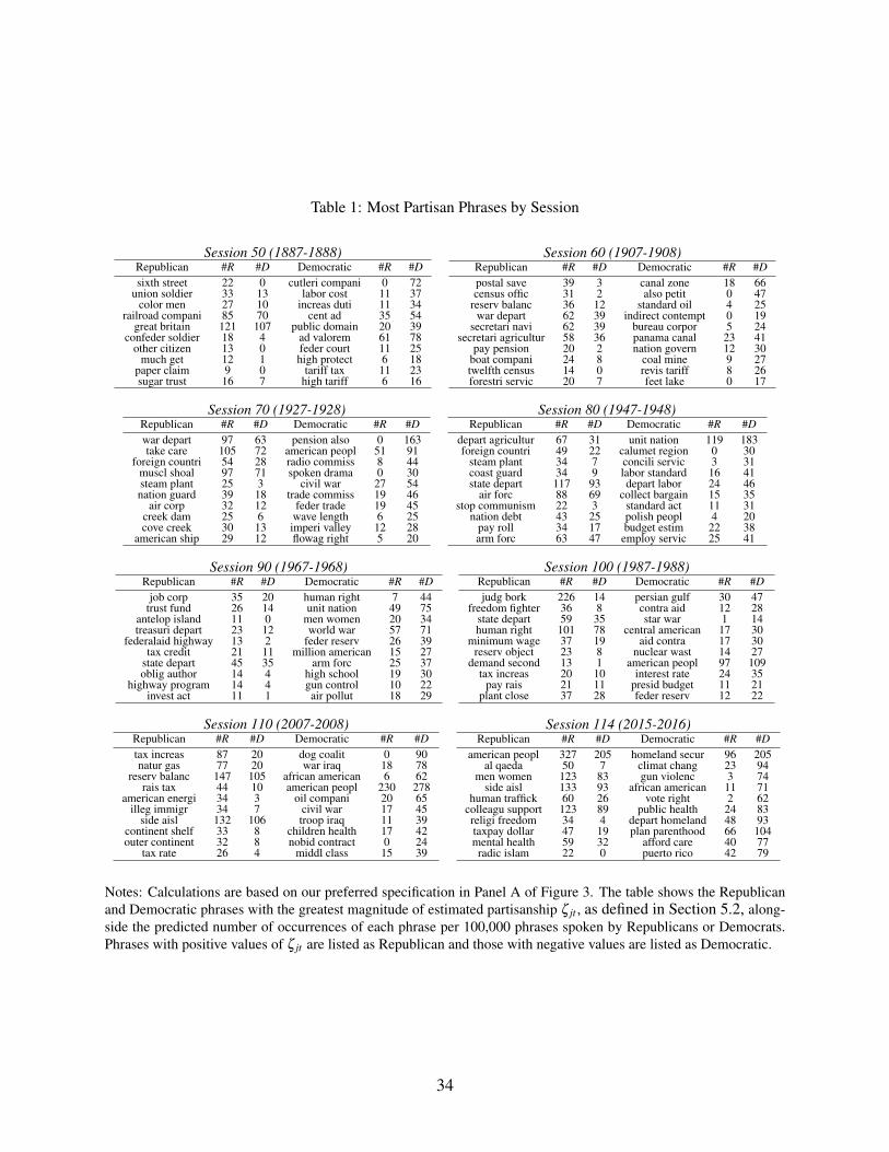
Table 1: Most Partisan Phrases by Session

Session 50 (1887-1888)Republican #R #D Democratic #R #Dsixth street 22 0 cutleri compani 0 72

union soldier 33 13 labor cost 11 37color men 27 10 increas duti 11 34

railroad compani 85 70 cent ad 35 54great britain 121 107 public domain 20 39

confeder soldier 18 4 ad valorem 61 78other citizen 13 0 feder court 11 25

much get 12 1 high protect 6 18paper claim 9 0 tariff tax 11 23sugar trust 16 7 high tariff 6 16

Session 60 (1907-1908)Republican #R #D Democratic #R #Dpostal save 39 3 canal zone 18 66census offic 31 2 also petit 0 47

reserv balanc 36 12 standard oil 4 25war depart 62 39 indirect contempt 0 19

secretari navi 62 39 bureau corpor 5 24secretari agricultur 58 36 panama canal 23 41

pay pension 20 2 nation govern 12 30boat compani 24 8 coal mine 9 27twelfth census 14 0 revis tariff 8 26forestri servic 20 7 feet lake 0 17

Session 70 (1927-1928)Republican #R #D Democratic #R #Dwar depart 97 63 pension also 0 163take care 105 72 american peopl 51 91

foreign countri 54 28 radio commiss 8 44muscl shoal 97 71 spoken drama 0 30steam plant 25 3 civil war 27 54nation guard 39 18 trade commiss 19 46

air corp 32 12 feder trade 19 45creek dam 25 6 wave length 6 25cove creek 30 13 imperi valley 12 28

american ship 29 12 flowag right 5 20

Session 80 (1947-1948)Republican #R #D Democratic #R #D

depart agricultur 67 31 unit nation 119 183foreign countri 49 22 calumet region 0 30

steam plant 34 7 concili servic 3 31coast guard 34 9 labor standard 16 41state depart 117 93 depart labor 24 46

air forc 88 69 collect bargain 15 35stop communism 22 3 standard act 11 31

nation debt 43 25 polish peopl 4 20pay roll 34 17 budget estim 22 38arm forc 63 47 employ servic 25 41

Session 90 (1967-1968)Republican #R #D Democratic #R #D

job corp 35 20 human right 7 44trust fund 26 14 unit nation 49 75

antelop island 11 0 men women 20 34treasuri depart 23 12 world war 57 71

federalaid highway 13 2 feder reserv 26 39tax credit 21 11 million american 15 27

state depart 45 35 arm forc 25 37oblig author 14 4 high school 19 30

highway program 14 4 gun control 10 22invest act 11 1 air pollut 18 29

Session 100 (1987-1988)Republican #R #D Democratic #R #Djudg bork 226 14 persian gulf 30 47

freedom fighter 36 8 contra aid 12 28state depart 59 35 star war 1 14human right 101 78 central american 17 30

minimum wage 37 19 aid contra 17 30reserv object 23 8 nuclear wast 14 27

demand second 13 1 american peopl 97 109tax increas 20 10 interest rate 24 35

pay rais 21 11 presid budget 11 21plant close 37 28 feder reserv 12 22

Session 110 (2007-2008)Republican #R #D Democratic #R #Dtax increas 87 20 dog coalit 0 90natur gas 77 20 war iraq 18 78

reserv balanc 147 105 african american 6 62rais tax 44 10 american peopl 230 278

american energi 34 3 oil compani 20 65illeg immigr 34 7 civil war 17 45

side aisl 132 106 troop iraq 11 39continent shelf 33 8 children health 17 42outer continent 32 8 nobid contract 0 24

tax rate 26 4 middl class 15 39

Session 114 (2015-2016)Republican #R #D Democratic #R #D

american peopl 327 205 homeland secur 96 205al qaeda 50 7 climat chang 23 94

men women 123 83 gun violenc 3 74side aisl 133 93 african american 11 71

human traffick 60 26 vote right 2 62colleagu support 123 89 public health 24 83religi freedom 34 4 depart homeland 48 93taxpay dollar 47 19 plan parenthood 66 104mental health 59 32 afford care 40 77radic islam 22 0 puerto rico 42 79

Notes: Calculations are based on our preferred specification in Panel A of Figure 3. The table shows the Republicanand Democratic phrases with the greatest magnitude of estimated partisanship ζ jt , as defined in Section 5.2, along-side the predicted number of occurrences of each phrase per 100,000 phrases spoken by Republicans or Democrats.Phrases with positive values of ζ jt are listed as Republican and those with negative values are listed as Democratic.

34

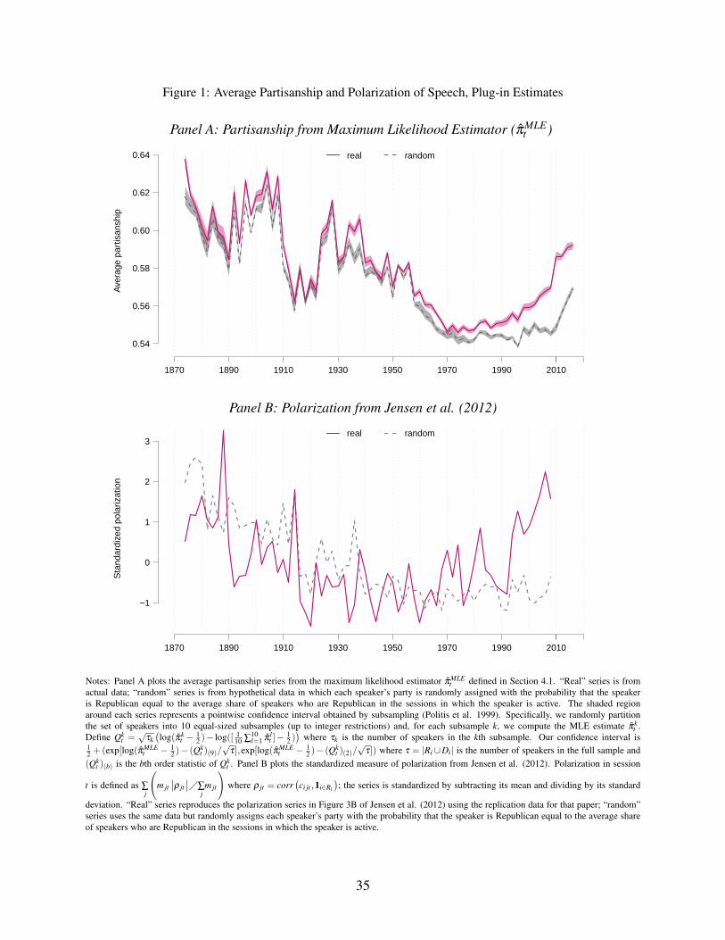
Figure 1: Average Partisanship and Polarization of Speech, Plug-in Estimates

Panel A: Partisanship from Maximum Likelihood Estimator (π̂MLEt )

Ave

rage

par

tisan

ship

1870 1890 1910 1930 1950 1970 1990 2010

0.54

0.56

0.58

0.60

0.62

0.64 real random

Panel B: Polarization from Jensen et al. (2012)

Sta

ndar

dize

d po

lariz

atio

n

1870 1890 1910 1930 1950 1970 1990 2010

−1

0

1

2

3real random

Notes: Panel A plots the average partisanship series from the maximum likelihood estimator π̂MLEt defined in Section 4.1. “Real” series is from

actual data; “random” series is from hypothetical data in which each speaker’s party is randomly assigned with the probability that the speakeris Republican equal to the average share of speakers who are Republican in the sessions in which the speaker is active. The shaded regionaround each series represents a pointwise confidence interval obtained by subsampling (Politis et al. 1999). Specifically, we randomly partitionthe set of speakers into 10 equal-sized subsamples (up to integer restrictions) and, for each subsample k, we compute the MLE estimate π̂k

t .Define Qk

t =√

τk(log(π̂k

t − 12 )− log([ 1

10 ∑10l=1 π̂ l

t ]− 12 ))

where τk is the number of speakers in the kth subsample. Our confidence interval is12 +(exp[log(π̂MLE

t − 12 )− (Qk

t )(9)/√

τ],exp[log(π̂MLEt − 1

2 )− (Qkt )(2)/

√τ]) where τ = |Ri ∪Di| is the number of speakers in the full sample and

(Qkt )(b) is the bth order statistic of Qk

t . Panel B plots the standardized measure of polarization from Jensen et al. (2012). Polarization in session

t is defined as ∑j

(m jt∣∣ρ jt∣∣�∑

jm jt

)where ρ jt = corr

(ci jt ,1i∈Rt

); the series is standardized by subtracting its mean and dividing by its standard

deviation. “Real” series reproduces the polarization series in Figure 3B of Jensen et al. (2012) using the replication data for that paper; “random”series uses the same data but randomly assigns each speaker’s party with the probability that the speaker is Republican equal to the average shareof speakers who are Republican in the sessions in which the speaker is active.

35

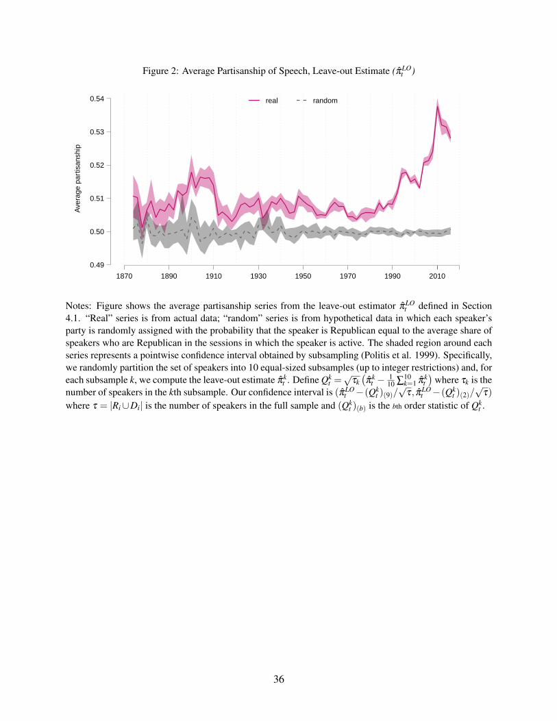
Figure 2: Average Partisanship of Speech, Leave-out Estimate (π̂LOt )

Ave

rage

par

tisan

ship

1870 1890 1910 1930 1950 1970 1990 2010

0.49

0.50

0.51

0.52

0.53

0.54 real random

Notes: Figure shows the average partisanship series from the leave-out estimator π̂LOt defined in Section

4.1. “Real” series is from actual data; “random” series is from hypothetical data in which each speaker’sparty is randomly assigned with the probability that the speaker is Republican equal to the average share ofspeakers who are Republican in the sessions in which the speaker is active. The shaded region around eachseries represents a pointwise confidence interval obtained by subsampling (Politis et al. 1999). Specifically,we randomly partition the set of speakers into 10 equal-sized subsamples (up to integer restrictions) and, foreach subsample k, we compute the leave-out estimate π̂k

t . Define Qkt =√

τk(π̂k

t − 110 ∑

10k=1 π̂k

t)

where τk is thenumber of speakers in the kth subsample. Our confidence interval is (π̂LO

t −(Qkt )(9)/

√τ, π̂LO

t −(Qkt )(2)/

√τ)

where τ = |Ri∪Di| is the number of speakers in the full sample and (Qkt )(b) is the bth order statistic of Qk

t .

36

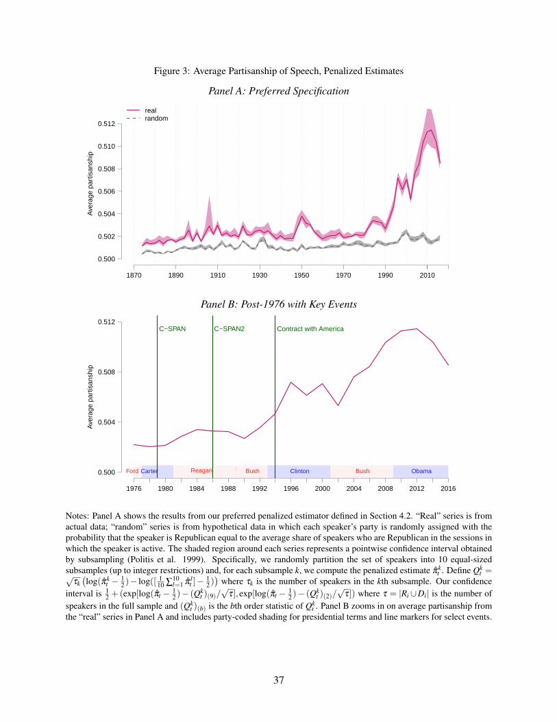
Figure 3: Average Partisanship of Speech, Penalized Estimates

Panel A: Preferred SpecificationA

vera

ge p

artis

ansh

ip

1870 1890 1910 1930 1950 1970 1990 2010

0.500

0.502

0.504

0.506

0.508

0.510

0.512

realrandom

Panel B: Post-1976 with Key Events

Ave

rage

par

tisan

ship

1976 1980 1984 1988 1992 1996 2000 2004 2008 2012 2016

0.500

0.504

0.508

0.512C−SPAN C−SPAN2 Contract with America

Ford Carter Reagan Bush Clinton Bush Obama

Notes: Panel A shows the results from our preferred penalized estimator defined in Section 4.2. “Real” series is fromactual data; “random” series is from hypothetical data in which each speaker’s party is randomly assigned with theprobability that the speaker is Republican equal to the average share of speakers who are Republican in the sessions inwhich the speaker is active. The shaded region around each series represents a pointwise confidence interval obtainedby subsampling (Politis et al. 1999). Specifically, we randomly partition the set of speakers into 10 equal-sizedsubsamples (up to integer restrictions) and, for each subsample k, we compute the penalized estimate π̂k

t . Define Qkt =√

τk(log(π̂k

t − 12 )− log([ 1

10 ∑10l=1 π̂ l

t ]− 12 ))

where τk is the number of speakers in the kth subsample. Our confidenceinterval is 1

2 +(exp[log(π̂t − 12 )− (Qk

t )(9)/√

τ],exp[log(π̂t − 12 )− (Qk

t )(2)/√

τ]) where τ = |Ri∪Di| is the number ofspeakers in the full sample and (Qk

t )(b) is the bth order statistic of Qkt . Panel B zooms in on average partisanship from

the “real” series in Panel A and includes party-coded shading for presidential terms and line markers for select events.

37

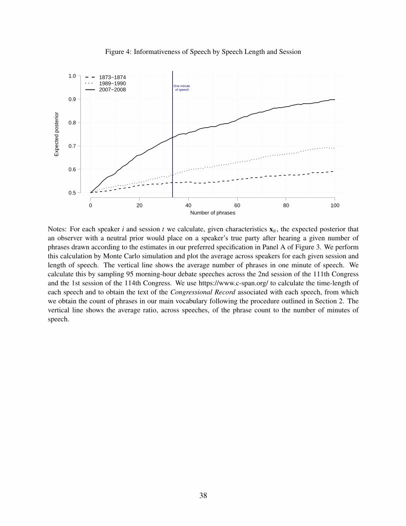
Figure 4: Informativeness of Speech by Speech Length and SessionE

xpec

ted

post

erio

r

0 20 40 60 80 100

0.5

0.6

0.7

0.8

0.9

1.0

Number of phrases

One minute of speech

1873−18741989−19902007−2008

Notes: For each speaker i and session t we calculate, given characteristics xit , the expected posterior thatan observer with a neutral prior would place on a speaker’s true party after hearing a given number ofphrases drawn according to the estimates in our preferred specification in Panel A of Figure 3. We performthis calculation by Monte Carlo simulation and plot the average across speakers for each given session andlength of speech. The vertical line shows the average number of phrases in one minute of speech. Wecalculate this by sampling 95 morning-hour debate speeches across the 2nd session of the 111th Congressand the 1st session of the 114th Congress. We use https://www.c-span.org/ to calculate the time-length ofeach speech and to obtain the text of the Congressional Record associated with each speech, from whichwe obtain the count of phrases in our main vocabulary following the procedure outlined in Section 2. Thevertical line shows the average ratio, across speeches, of the phrase count to the number of minutes ofspeech.

38

Figure 5: Partisanship vs. Roll-Call Voting

Panel A: Over Time

1870 1890 1910 1930 1950 1970 1990 2010

0.500

0.502

0.504

0.506

0.508

0.510

0.512

0.50

0.55

0.60

0.65

0.70

0.75

0.80

0.85

0.90average partisanship (speech)distance between parties (roll−call voting)

Panel B: Across Speakers

.44

.46

.48

.5

.52

.54

.56

−1.0 −0.5 0.0 0.5 1.0

NOMINATE

Par

tisan

ship

Democrat

Republican

Notes: Panel A shows our preferred estimate of average partisanship from Panel A of Figure 3 and the difference be-tween the average Republican and the average Democrat in the first dimension of the Common Space DW-NOMINATEscore from McCarty et al. (2015). Panel B plots a speaker’s posterior probability ρ̂i of being Republican based onspeech against the first dimension of the Common Space DW-NOMINATE score (McCarty et al. 2015). We dropobservations for which we cannot match a DW-NOMINATE score to the speaker. To compute ρ̂i, we first defineρ̂it = q̂it · ρ̂ρρ∗t (xit), where we recall that q̂it = cit/mit are the empirical phrase frequencies for speaker i in session tand where we define ρ̂ρρ

∗t (xit) as the estimated value of ρρρ t (xit) from our baseline penalized estimates. We then let

ρ̂i =1|Ti| ∑t∈Ti ρ̂it where Ti is the set of all sessions in which speaker i appears. Nine outliers are excluded from the plot.

The solid black line denotes the linear best fit among the points plotted.

39

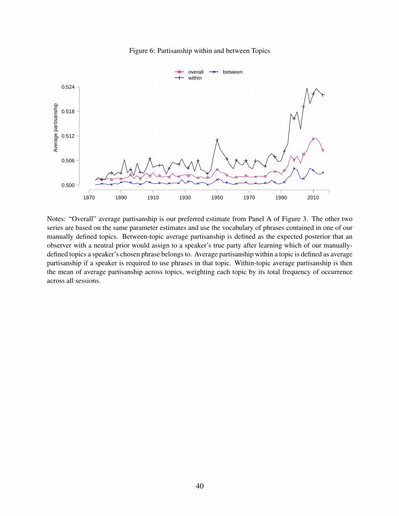
Figure 6: Partisanship within and between TopicsA

vera

ge p

artis

ansh

ip

1870 1890 1910 1930 1950 1970 1990 2010

0.500

0.506

0.512

0.518

0.524

overallwithin

between

Notes: “Overall” average partisanship is our preferred estimate from Panel A of Figure 3. The other twoseries are based on the same parameter estimates and use the vocabulary of phrases contained in one of ourmanually defined topics. Between-topic average partisanship is defined as the expected posterior that anobserver with a neutral prior would assign to a speaker’s true party after learning which of our manually-defined topics a speaker’s chosen phrase belongs to. Average partisanship within a topic is defined as averagepartisanship if a speaker is required to use phrases in that topic. Within-topic average partisanship is thenthe mean of average partisanship across topics, weighting each topic by its total frequency of occurrenceacross all sessions.

40

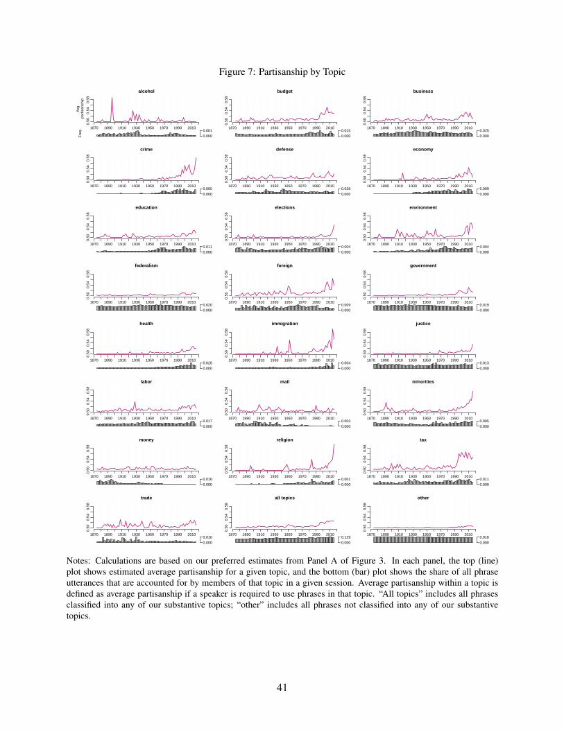
Figure 7: Partisanship by Topic0.

500.

540.

58alcohol

1870 1890 1910 1930 1950 1970 1990 2010

Avg

.pa

rtis

ansh

ip

0.50

0.54

0.58

budget

1870 1890 1910 1930 1950 1970 1990 2010

0.50

0.54

0.58

business

1870 1890 1910 1930 1950 1970 1990 2010

0.000

0.001

Fre

q.

0.000

0.015

0.000

0.025

0.50

0.54

0.58

crime

1870 1890 1910 1930 1950 1970 1990 2010

0.50

0.54

0.58

defense

1870 1890 1910 1930 1950 1970 1990 2010

0.50

0.54

0.58

economy

1870 1890 1910 1930 1950 1970 1990 2010

0.000

0.005

0.000

0.028

0.000

0.009

0.50

0.54

0.58

education

1870 1890 1910 1930 1950 1970 1990 2010

0.50

0.54

0.58

elections

1870 1890 1910 1930 1950 1970 1990 2010

0.50

0.54

0.58

environment

1870 1890 1910 1930 1950 1970 1990 2010

0.000

0.011

0.000

0.004

0.000

0.004

0.50

0.54

0.58

federalism

1870 1890 1910 1930 1950 1970 1990 2010

0.50

0.54

0.58

foreign

1870 1890 1910 1930 1950 1970 1990 2010

0.50

0.54

0.58

government

1870 1890 1910 1930 1950 1970 1990 2010

0.000

0.020

0.000

0.009

0.000

0.019

0.50

0.54

0.58

health

1870 1890 1910 1930 1950 1970 1990 2010

0.50

0.54

0.58

immigration

1870 1890 1910 1930 1950 1970 1990 20100.

500.

540.

58

justice

1870 1890 1910 1930 1950 1970 1990 2010

0.000

0.028

0.000

0.004

0.000

0.013

0.50

0.54

0.58

labor

1870 1890 1910 1930 1950 1970 1990 2010

0.50

0.54

0.58

mail

1870 1890 1910 1930 1950 1970 1990 2010

0.50

0.54

0.58

minorities

1870 1890 1910 1930 1950 1970 1990 2010

0.000

0.017

0.000

0.003

0.000

0.005

0.50

0.54

0.58

money

1870 1890 1910 1930 1950 1970 1990 2010

0.50

0.54

0.58

religion

1870 1890 1910 1930 1950 1970 1990 2010

0.50

0.54

0.58

tax

1870 1890 1910 1930 1950 1970 1990 2010

0.000

0.016

0.000

0.001

0.000

0.011

0.50

0.54

0.58

trade

1870 1890 1910 1930 1950 1970 1990 2010

0.50

0.54

0.58

all topics

1870 1890 1910 1930 1950 1970 1990 2010

0.50

0.54

0.58

other

1870 1890 1910 1930 1950 1970 1990 2010

0.000

0.010

0.000

0.129

0.000

0.918

Notes: Calculations are based on our preferred estimates from Panel A of Figure 3. In each panel, the top (line)plot shows estimated average partisanship for a given topic, and the bottom (bar) plot shows the share of all phraseutterances that are accounted for by members of that topic in a given session. Average partisanship within a topic isdefined as average partisanship if a speaker is required to use phrases in that topic. “All topics” includes all phrasesclassified into any of our substantive topics; “other” includes all phrases not classified into any of our substantivetopics.

41

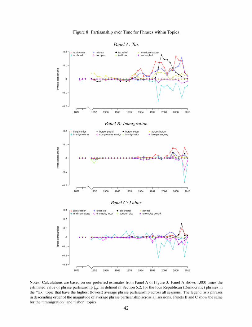
Figure 8: Partisanship over Time for Phrases within Topics

Panel A: Tax

Phr

ase

part

isan

ship

−0.2

−0.1

0

0.1

0.2

1872 1952 1960 1968 1976 1984 1992 2000 2008 2016

● ● ● ●●

● ●

● ● ● ● ● ●

●

●

●

●

●●

●●

●● ●

●

●

●

●

● ●

●

●

●

●

●

● ●

●tax increastax break

rais taxtax upon

tax relieftariff tax

american taxpaytax loophol

Panel B: Immigration

Phr

ase

part

isan

ship

−0.2

−0.1

0

0.1

0.2

1872 1952 1960 1968 1976 1984 1992 2000 2008 2016

● ● ● ● ● ● ● ● ● ● ● ● ● ● ● ● ● ● ● ● ● ● ● ● ● ● ● ● ● ● ●

●

● ● ●

●

●

●illeg immigrimmigr reform

border patrolcomprehens immigr

border securimmigr natur

across borderforeign languag

Panel C: Labor

Phr

ase

part

isan

ship

−0.3

−0.2

−0.1

0

0.1

0.2

0.3

1872 1952 1960 1968 1976 1984 1992 2000 2008 2016

● ● ● ● ● ● ● ● ● ● ● ● ● ● ● ● ● ● ● ● ● ● ● ● ● ● ● ● ● ●● ● ●

●

●

● ●

●job creationminimum wage

creat jobunemploy insur

job creatorpension also

pay rollunemploy benefit

Notes: Calculations are based on our preferred estimates from Panel A of Figure 3. Panel A shows 1,000 times theestimated value of phrase partisanship ζ jt , as defined in Section 5.2, for the four Republican (Democratic) phrases inthe “tax” topic that have the highest (lowest) average phrase partisanship across all sessions. The legend lists phrasesin descending order of the magnitude of average phrase partisanship across all sessions. Panels B and C show the samefor the “immigration” and “labor” topics.

42

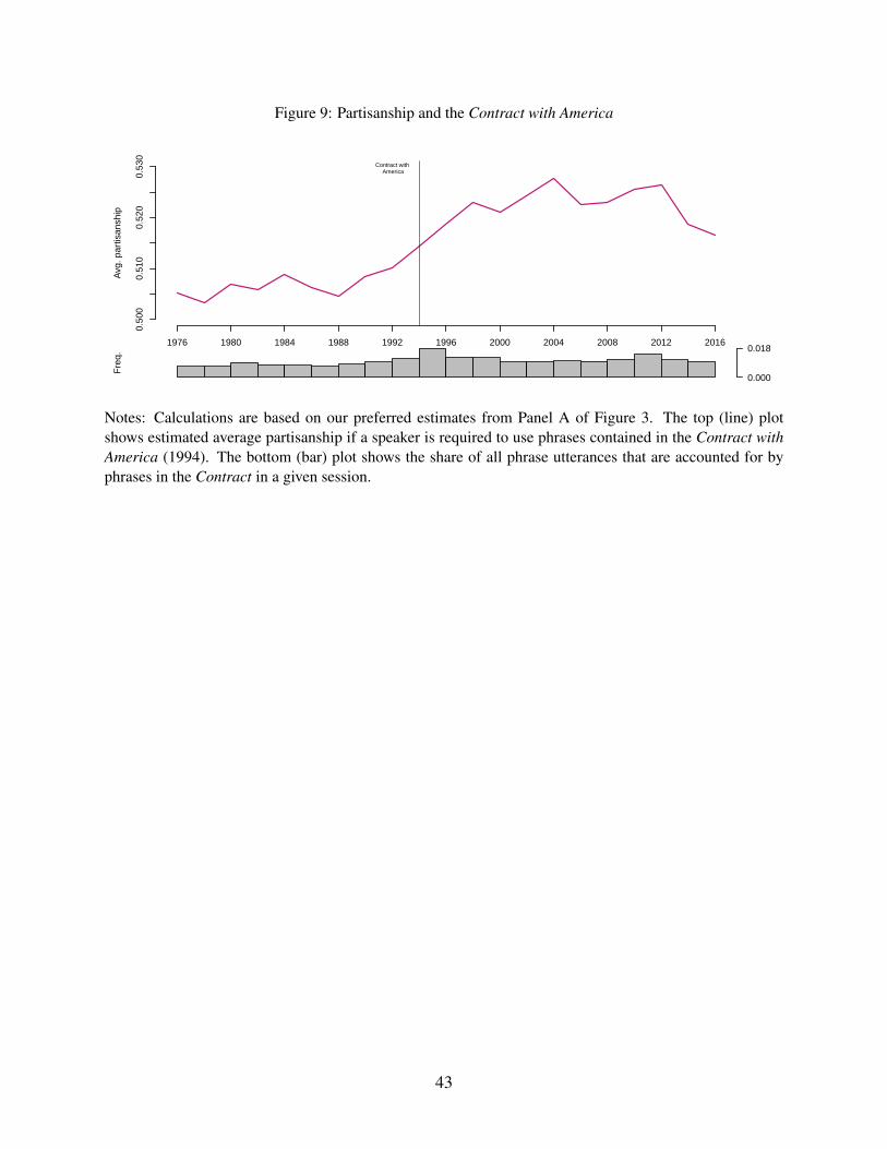
Figure 9: Partisanship and the Contract with America

0.50

00.

510

0.52

00.

530

1976 1980 1984 1988 1992 1996 2000 2004 2008 2012 2016

Avg

. par

tisan

ship

Contract with America

0.000

0.018

Fre

q.

Notes: Calculations are based on our preferred estimates from Panel A of Figure 3. The top (line) plotshows estimated average partisanship if a speaker is required to use phrases contained in the Contract withAmerica (1994). The bottom (bar) plot shows the share of all phrase utterances that are accounted for byphrases in the Contract in a given session.

43

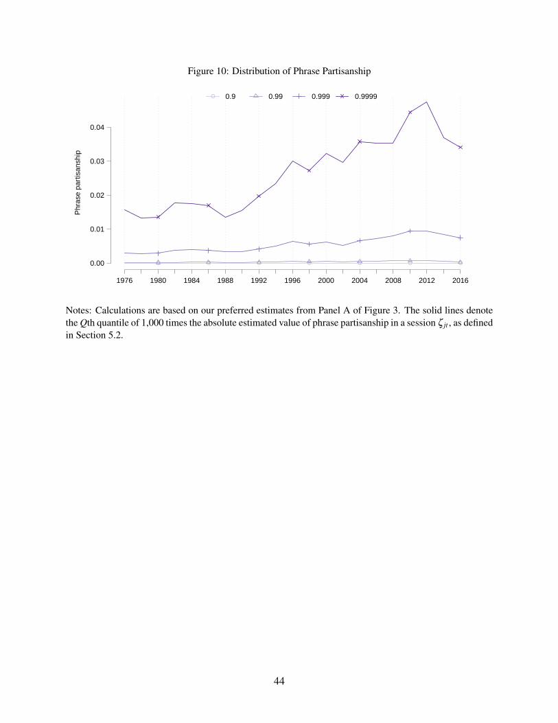
Figure 10: Distribution of Phrase PartisanshipP

hras

e pa

rtis

ansh

ip

1976 1980 1984 1988 1992 1996 2000 2004 2008 2012 2016

0.00

0.01

0.02

0.03

0.04

● ● ● ● ● ● ●

● 0.9 0.99 0.999 0.9999

Notes: Calculations are based on our preferred estimates from Panel A of Figure 3. The solid lines denotethe Qth quantile of 1,000 times the absolute estimated value of phrase partisanship in a session ζ jt , as definedin Section 5.2.

44

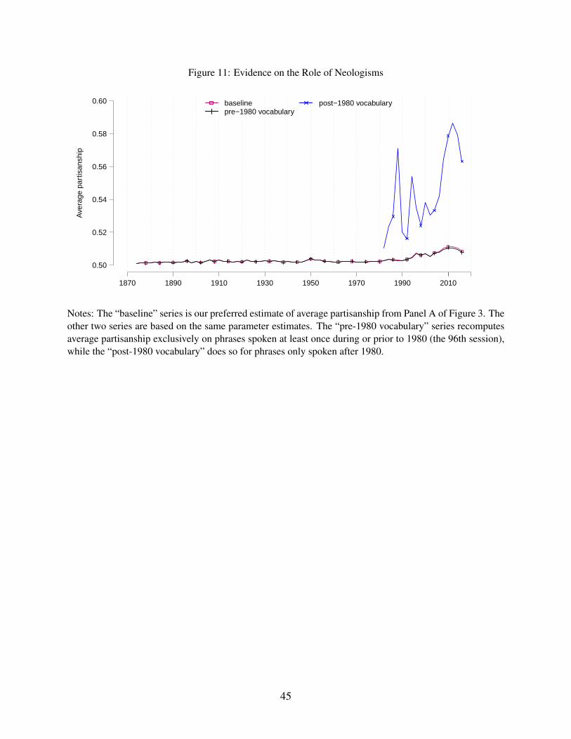
Figure 11: Evidence on the Role of NeologismsA

vera

ge p

artis

ansh

ip

1870 1890 1910 1930 1950 1970 1990 2010

0.50

0.52

0.54

0.56

0.58

0.60 baselinepre−1980 vocabulary

post−1980 vocabulary

Notes: The “baseline” series is our preferred estimate of average partisanship from Panel A of Figure 3. Theother two series are based on the same parameter estimates. The “pre-1980 vocabulary” series recomputesaverage partisanship exclusively on phrases spoken at least once during or prior to 1980 (the 96th session),while the “post-1980 vocabulary” does so for phrases only spoken after 1980.

45

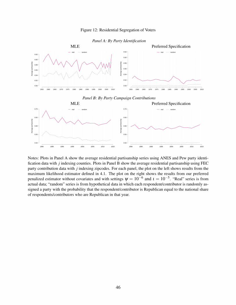
Figure 12: Residential Segregation of Voters

Panel A: By Party IdentificationMLE Preferred Specification

Ave

rage

par

tisan

ship

1955 1960 1965 1970 1975 1980 1985 1990 1995 2000 2005 2010

0.50

0.52

0.54

0.56

0.58

0.60

0.62real random

Ave

rage

par

tisan

ship

1955 1960 1965 1970 1975 1980 1985 1990 1995 2000 2005 2010

0.50

0.52

0.54

0.56

0.58

0.60

0.62 real random

Panel B: By Party Campaign ContributionsMLE Preferred Specification

Ave

rage

par

tisan

ship

1980 1985 1990 1995 2000 2005 2010 2015

0.50

0.55

0.60

0.65

0.70 real random

Ave

rage

par

tisan

ship

1980 1985 1990 1995 2000 2005 2010 2015

0.50

0.55

0.60

0.65

0.70 real random

Notes: Plots in Panel A show the average residential partisanship series using ANES and Pew party identi-fication data with j indexing counties. Plots in Panel B show the average residential partisanship using FECparty contribution data with j indexing zipcodes. For each panel, the plot on the left shows results from themaximum likelihood estimator defined in 4.1. The plot on the right shows the results from our preferredpenalized estimator without covariates and with settings ψ = 10−6 and ι = 10−5. “Real” series is fromactual data; “random” series is from hypothetical data in which each respondent/contributor is randomly as-signed a party with the probability that the respondent/contributor is Republican equal to the national shareof respondents/contributors who are Republican in that year.

46