Vibration Measurement and Prediction for Foundation Slab ...

1
MEASUREMENT AND PREDICTION OF THE
LOAD DISTRIBUTION AND PERFORMANCE
OF CONTINUOUS FLIGHT AUGER PILES
by
Thomas Leon Pine
BEng, BComm
This Thesis is presented for the Degree of Master of Engineering Science of the
University of Western Australia
School of Civil, Mining and Environmental Engineering
Civil Engineering
July 2016

3
Abstract
It is becoming increasingly important to not only reliably predict a pile’s ultimate load but to
also predict a piles load-displacement behaviour. In order to predict this behaviour, it is
imperative that the contribution of shaft friction and base load to the overall capacity can be
measured accurately. To determine the relative contributions in bored piles, strain gauged static
load tests are a commonly used. Their application and interpretation is not, however, as
straightforward as is often believed.
This thesis examines the measurement and prediction of load distribution and performance of
bored piles using a range of pile load tests recently performed by the author at a number of sites
in Perth, Australia. A number of analysis methods outlined in Lam and Jefferis (2011),
including the Tangent Method proposed by Fellenius (1989, 2001), are examined and applied to
the field tests. Insights into the strengths and weaknesses are provided in the thesis. The
increased insight that the Tangent Method provided to one case history suggests that it should
be considered in future instrumented test piles.
A load transfer program, referred to as RATZ, is used to derive parameters that gave a best fit to
the pile load-displacement data. Correlation with CPT resistances are examined and discussed,
and shown to be a reliable means of predicting pile axial response.

4
Table of Contents
1 Introduction ......................................................................................................................... 12
The need for pile research ........................................................................................... 12
Assessment of the axial response of bored piles ......................................................... 13
1.3 Primary objectives of thesis ......................................................................................... 14
1.4 Thesis Outline .............................................................................................................. 14
2 Literature Review ................................................................................................................ 16
Determination of Load Distribution from Static Load Tests ....................................... 16
2.1.1 Fundamentals ....................................................................................................... 16
2.1.2 Cross Sectional Area of a Bored Pile .................................................................. 16
2.1.3 Modulus of Elasticity of Concrete / Grout .......................................................... 18
2.1.4 Measuring Strain.................................................................................................. 20
2.1.5 Methods of converting strain to load ................................................................... 23
2.1.6 Stress to Shaft Friction ........................................................................................ 26
Parameter Selection for Bored Piles in Sand ............................................................... 28
2.2.1 Pile Capacity Fundamentals ................................................................................ 28
2.2.2 Pile Deformation Fundamentals .......................................................................... 29
2.2.3 RATZ ................................................................................................................... 31
2.2.4 Cone Penetrometer Test ....................................................................................... 33
2.2.5 Shaft Friction at Failure Correlations .................................................................. 36
2.2.6 Shear Modulus of Sand (G) ................................................................................. 37
2.2.7 Pile Base Capacity ............................................................................................... 38
3 Test Sites ............................................................................................................................. 41
500 Hay St Subiaco ..................................................................................................... 42
3.1.1 Location ............................................................................................................... 42
3.1.2 Ground Conditions .............................................................................................. 43
3.1.3 Test Pile Details ................................................................................................... 44
3.1.4 Testing Procedure and results .............................................................................. 45
Cloisters Redevelopment ............................................................................................. 48
3.2.1 Location ............................................................................................................... 48

5
3.2.2 Ground Conditions .............................................................................................. 48
3.2.3 Test Pile Details .................................................................................................. 50
3.2.4 Testing Procedure and Results ............................................................................ 51
Cockburn Gateway Shopping Centre .......................................................................... 53
3.3.1 Location .............................................................................................................. 53
3.3.2 Ground Conditions .............................................................................................. 54
3.3.3 Test Pile Details .................................................................................................. 54
3.3.4 Testing Procedure and Results ............................................................................ 56
999 Hay St, Perth ........................................................................................................ 59
3.4.1 Location .............................................................................................................. 59
3.4.2 Ground Conditions .............................................................................................. 60
3.4.3 Test Pile Details .................................................................................................. 61
3.4.4 Testing Procedure and Results ............................................................................ 61
UWA IOMRC ............................................................................................................. 64
3.5.1 Location .............................................................................................................. 64
3.5.2 Ground Conditions .............................................................................................. 65
3.5.3 Test Pile Details .................................................................................................. 66
3.5.4 Testing Procedure and Results ............................................................................ 66
4 Measuring Load Distribution in Bored Piles ...................................................................... 70
4.1.1 500 Hay St Strain Gauge Analysis ...................................................................... 70
4.1.2 Uncorrected Area Method ................................................................................... 71
4.1.3 Transformed Area Method .................................................................................. 72
4.1.4 Implicit Method................................................................................................... 73
4.1.5 Secant Modulus Method ..................................................................................... 74
4.1.6 Tangent Modulus Method ................................................................................... 75
4.1.7 Comparison ......................................................................................................... 80
Cloisters Redevelopment Strain Gauge Analysis ....................................................... 82
4.2.1 Uncorrected Area Method ................................................................................... 82
4.2.2 Transformed Area Method .................................................................................. 83
4.2.3 Implicit Method................................................................................................... 84
6
4.2.4 Secant Modulus Method ...................................................................................... 84
4.2.5 Tangent Method ................................................................................................... 86
4.2.6 Comparison .......................................................................................................... 87
Cockburn Gateway TP1 Strain Gauge Analysis .......................................................... 89
4.3.1 Uncorrected Area Method ................................................................................... 90
4.3.2 Other Methods ..................................................................................................... 92
4.3.3 Tangent Method ................................................................................................... 92
4.3.4 Uncorrected Area Method with 3.5m and 7.5m Switched .................................. 95
4.3.5 Summary .............................................................................................................. 96
Cockburn TP2 Strain Gauge Analysis ......................................................................... 97
4.4.1 Uncorrected Area Method ................................................................................... 98
4.4.2 Transformed Area Method .................................................................................. 99
4.4.3 Implicit Method ................................................................................................. 100
4.4.4 Secant Modulus Method .................................................................................... 100
4.4.5 Tangent Method ................................................................................................. 102
4.4.6 Comparison ........................................................................................................ 104
5 Pile Performance Parameter Selection .............................................................................. 107
500 Hay St Pile Parameters ....................................................................................... 107
5.1.1 Corrections for Axial Compression for Segment Analyses ............................... 107
5.1.2 Modelling Individual Segments Shaft Response in RATZ ............................... 110
5.1.3 Overall Shaft Friction Response ........................................................................ 114
5.1.4 Comparison of τp CPT qc Values ....................................................................... 115
5.1.5 Comparison of GRATZ CPT qc Values ................................................................ 116
5.1.6 Base Response ................................................................................................... 118
5.1.7 CPT Tip resistance to ultimate base pressure .................................................... 120
5.1.8 Overall Pile RATZ Model ................................................................................. 121
Application to Other Tests ......................................................................................... 122
5.2.1 UWA Load Test TP1, Crawley WA .................................................................. 122
5.2.2 UWA Load Test TP2, Crawley WA .................................................................. 124
5.2.3 999 Hay St Perth ................................................................................................ 125

7
6 Conclusions ....................................................................................................................... 127
Determination of load distribution from strain gauge data ....................................... 127
Correlating pile performance to CPT results ............................................................ 128
7 References ......................................................................................................................... 129

8
Figure 2.1: Calculated load errors resulting from pile diameter variation ................................... 17
Figure 2.2: Illustration of effect of pile diameter on the apparent Modulus of Elasticity ........... 17
Figure 2.3: Non-Linear stress vs normalised strain for local concrete specimen ........................ 19
Figure 2.4: Young’s Modulus vs w/c ratio for neat cement grouts (Hyen et al. 1992) ............... 20
Figure 2.5: Geokon 3911A Strain Gauge Sister bars .................................................................. 21
Figure 2.6: Typical normalised shaft friction vs displacement curves (Reece and Oneil 1988) . 25
Figure 2.7: Shaft friction t-z curves from SSTs on small dia. Jacked steel tubes ........................ 26
Figure 2.8: Summary of Analysis Methods from Lam (2011) .................................................... 27
Figure 2.9: RATZ shaft load transfer curve ................................................................................ 32
Figure 2.10:Typical CPT Cone .................................................................................................... 34
Figure 2.11:CPT qc relationship to Dr (Baldi et al 1988) ............................................................ 35
Figure 2.12: CPT qc relationship to pile shaft friction (De Cock) ............................................... 37
Figure 2.13: Self Boring Pressuremeter Test results at a Perth Sand Site (Fahey 2007) ............. 38
Figure 3.1: Location of Test Sites in the Perth Metropolitan region ........................................... 41
Figure 3.2: 500 Hay St Test Area Location ................................................................................. 42
Figure 3.3: 500 Hay St Test Area Detailed Layout ..................................................................... 43
Figure 3.4: 500 Hay St Subiaco Test Pile CPTs .......................................................................... 44
Figure 3.5: 500 Hay St Pile Test Setup ....................................................................................... 46
Figure 3.6: 500 Hay Sy Load Test Load vs Displacement Curve ............................................... 47
Figure 3.7: 500 Hay St Test Loading Schedule ........................................................................... 47
Figure 3.8: Cloister Redevelopment Test Location ..................................................................... 48
Figure 3.9: Cloisters Redevelopment CPT Profiles ..................................................................... 49
Figure 3.10: Cloisters Redevelopment Test Layout .................................................................... 49
Figure 3.11: Cloisters Redevelopment Test Loading Rate .......................................................... 51
Figure 3.12: Cloisters Redevelopment Load Test Setup ............................................................. 51
Figure 3.13: Cloisters Redevelopment Test Load vs Displacement Plot .................................... 52
Figure 3.14: Cockburn Gateway Test Pile Location ................................................................... 53
Figure 3.15: Cockburn Gateway Test Layout ............................................................................. 53
Figure 3.16: Cockburn Gateway Test Pile CPTs ......................................................................... 54
Figure 3.17: Cockburn Gateway Pile Test Setup......................................................................... 56
Figure 3.18: Cockburn Gateway Test Loading Rates (left) TP1, (right) TP2 ............................. 57
Figure 3.19: Cockburn Gateway TP1 Load Displacement Curve ............................................... 57
Figure 3.20: Cockburn Gateway TP2 Load Displacement Curve ............................................... 58
Figure 3.21: 999 Hay St Test Location ........................................................................................ 59
Figure 3.22: 999 Hay St Test Pile Layout ................................................................................... 59
Figure 3.23: 999 Hay St Test Pile CPT ....................................................................................... 60
Figure 3.24: 999 Hay St Pile Loading Rate ................................................................................. 62
Figure 3.25: 999 Hay St Pile Test Setup ..................................................................................... 62

9
Figure 3.26: 999 Hay St Load vs Displacement Curve ............................................................... 63
Figure 3.27: UWA Test Locations .............................................................................................. 64
Figure 3.28: UWA Test Pile 1 Layout ........................................................................................ 64
Figure 3.29: UWA Test Pile 2 Layout ........................................................................................ 65
Figure 3.30: UWA Test CPTs ..................................................................................................... 65
Figure 3.31: UWA Load Test Setup (TP2) ................................................................................. 67
Figure 3.32: UWA Test Load Rate (left) TP1; (right) TP2......................................................... 67
Figure 3.33: UWA Test Load vs Displacement Curves .............................................................. 68
Figure 4.1: 500 Hay St Strain vs time ......................................................................................... 70
Figure 4.2: 500 Hay St Shaft friction vs head displacement determined using the un-corrected
area method ................................................................................................................................. 72
Figure 4.3: 500 Hay St Shaft friction vs head displacement determined using the implicit
method ........................................................................................................................................ 73
Figure 4.4: 500 Hay St Secant Modulus Top Strain Gauge trendline ......................................... 74
Figure 4.5: 500 Hay St Shaft friction vs head displacement determined using the secant method
.................................................................................................................................................... 75
Figure 4.6: 500 Hay St Tangent Modulus Raw Data Noise ........................................................ 76
Figure 4.7: 500 Hay St Strain at 0.5m Reduced to 50kN Steps .................................................. 77
Figure 4.8: 500 Hay St Tangent Method Line of best fits for the 5 strain gauge levels ............. 78
Figure 4.9: 500 Hay St Shaft friction vs head displacement determined using the tangent method
.................................................................................................................................................... 80
Figure 4.10: 500 Hay St Comparison of Strain Gauge Interpretation Methods .......................... 81
Figure 4.11: Cloisters Redevelopment Test Strain vs time ......................................................... 82
Figure 4.12: Cloisters Uncorrected Area Shaft Friction vs Head Displacement ........................ 83
Figure 4.13: Cloisters Secant Modulus Top Strain Trendline ..................................................... 85
Figure 4.14: Cloisters Secant Method Shaft Friction vs Head Displacement ............................. 85
Figure 4.15: Cloisters Tangent Method Modulus Plot ................................................................ 86
Figure 4.16: Cloisters Pile Head Load vs Strain ......................................................................... 87
Figure 4.17: Cloisters Test Interpretation Comparison ............................................................... 88
Figure 4.18: Cockburn TP1 Average Strain vs Time .................................................................. 89
Figure 4.19: Cockburn TP1 Uncorrected Area Predicted load at 1.5 vs head load..................... 91
Figure 4.20: Cockburn TP1 Uncorrected Area Shaft Friction vs Head Displacement ............... 92
Figure 4.21: Cockburn TP1 Tangent Plot vs head load for all individual gauges ...................... 93
Figure 4.23: Cockburn TP1 Tangent Method Plot vs head load for Averaged Strain Gauges ... 94
Figure 4.22: Cockburn TP1 Tangent Modulus vs Strain with Equivalent Secant Modulus Plotted
.................................................................................................................................................... 94
Figure 4.24: Cockburn TP1 Uncorrected Area Shaft Friction plot with the 3.5m and 7.5m
gauges switched .......................................................................................................................... 95

10
Figure 4.25: Cockburn TP2 Strain vs Time ................................................................................. 97
Figure 4.26: Cockburn TP2 Uncorrected Area Shaft Friction vs Head Displacement ................ 98
Figure 4.27: Cockburn TP2 Uncorrected Area Shaft Friction development ............................... 99
Figure 4.28: Cockburn TP2 Implicit Method Shaft Friction Development ............................... 100
Figure 4.29: Secant Modulus Top Strain Gauge trendline ........................................................ 101
Figure 4.30: Cockburn TP2 Secant Method Shaft Friction Development ................................. 102
Figure 4.31: Cockburn TP2 Tangent Method Plot .................................................................... 102
Figure 4.32 Cockburn TP2 Tangent Method Trendlines (a) 1.5m (b) 7.5m .............................. 103
Figure 4.33: Cockburn TP2 Tangent Method Shaft Friction Development .............................. 104
Figure 4.34: Cockburn TP2 Comparison of Interpretations ...................................................... 105
Figure 5.1: 500 Hay St Axial Compression Corrections for pile segment analyses .................. 108
Figure 5.2: 500 Hay St Corrected Shaft Friction vs Displacement ........................................... 109
Figure 5.3: Normalised Corrected Shaft Friction vs Displacement ........................................... 110
Figure 5.4: RATZ models plotted against test data for segment between 0.5m and 3.0m ........ 111
Figure 5.5: RATZ models plotted against test data for segment between 3.0m and 6.0m ........ 112
Figure 5.6: RATZ models plotted against test data for segment between 6.0m and 10.0m ...... 113
Figure 5.7: RATZ models plotted against test data for segment between 10.0m and 13.5m .... 114
Figure 5.8: RATZ models plotted against test data for overall shaft friction response ............. 115
Figure 5.9: 500 Hay St β vs Depth ............................................................................................ 116
Figure 5.10: 500 Hay St qc vs GRATZ ......................................................................................... 116
Figure 5.11: 500 Hay St CPT plots with friction sleeve and friction ratio data ........................ 117
Figure 5.12: 500 Hay St σ’v0 vs GRATZ....................................................................................... 118
Figure 5.13: 500 Hay St σ’v00.33. qc
0.33 . pATM0.33 vs GRATZ .......................................................... 118
Figure 5.14: 500 Hay St Pile Base Response ............................................................................ 119
Figure 5.15: 500 Hay St RATZ Base Response wb comparison ............................................... 120
Figure 5.16: 500 Hay St Test t-z Curve vs RATZ model .......................................................... 121
Figure 5.17: UWA TP1 Test vs RATZ Model ......................................................................... 122
Figure 5.18: UWA TP1 Test vs Modified RATZ Models ......................................................... 123
Figure 5.19: UWA TP2 Test vs RATZ Model .......................................................................... 124
Figure 5.20: 999 Hay St Test vs RATZ Model ......................................................................... 125

11
Chapter 1
Introduction

12
1 Introduction
The need for pile research
Complete building collapse is extremely rare in Australia. There are, however, piled structures
being designed and built today that continue to experience problems. This typically manifests
itself in the form of excessive settlements that affect the serviceability performance of the
structure and can require expensive remediation. Whilst problems are still occurring, it is
evident that there is still much to learn about piled foundations, in particular their in-service
performance.
As cities grow and age, their structures increase in complexity which increases the demand
placed on the performance of piles. For example:
- Buildings are getting taller which is increasing the pressure on the founding materials
- Basements are getting deeper which will deepen the foundations to zones in which
there is less experience
- the move to higher density living increases the interactions between the foundations of
adjacent structures
- The use of top down construction is increasing, which places greater emphasis on the
performance of piles and creates additional design problems
- Redevelopment and/or repair of old buildings which require the new structures to not
adversely affect the existing structures
These are all increasing the demand placed on the foundations of buildings which, without
sufficient experience and research, will typically manifest itself in two ways:
1. Increased conservatism and resulting increased cost of piled structures due to
uncertainties around performance; and/or
2. Increase in the occurrence of problematic issues because of insufficient design
practice.
It is becoming increasingly important to not only ensure that a pile has a satisfactory factor of
safety against failure but also that more accurate predictions about their performance (load
deformation response) are developed. As nearly every city around the world has its own set of
geological conditions, these pile performance predictions need to be calibrated to local
conditions.

13
Assessment of the axial response of bored piles
The primary way to accurately measure the performance of a pile is to conduct static load tests.
Static load tests provide direct measurement of a pile head load vs displacement which is what
the intended structure relies on. The problem with static load tests is that they do not usually
give a direct measurement of a pile’s shaft vs base response which is fundamental in pile design
equations. Without this load distribution, it is very difficult to confidently analyse a load test,
compare it to soil investigation data and then apply it to piles in other locations or of different
dimensions.
One way to obtain a measure of both the shaft and base response is to conduct an Osterberg Cell
test, which involves installing a hydraulic jack at a point in the pile (usually the base) to obtain
direct measurements of the load at that point. However, these tests are expensive and do not
obtain a direct measurement of head load vs displacement, rather an interpreted one as the upper
part of the pile is being pushed out of the ground.
Another approach is to conduct a static load test that includes embedded strain gauges to
measure the stress throughout the pile. This method relies on a knowledge of the relationship
between strain and stress, i.e. the Modulus of Elasticity or Young’s Modulus. In steel the
Young’s Modulus is well defined at around 200GPa and due to the manufacturing process the
area of the steel is well known. However, relating strain to stress in a concrete bored pile is not
as simple. Compared to steel, the Young’s Modulus of concrete is quite variable, being time and
rate dependent as well as depending on the concrete’s composition. In addition, depending on
the piling method chosen, the cross sectional area of the pile can also be subject to variability.
These uncertainties can lead to interpretation of a large range of shaft and base responses when
interpreting the data. This difficulty has likely assisted in the development of the wide range of
design parameters that are currently in use around the globe. This is why it is necessary to
examine ways in which strain gauges can be applied and analysed more effectively in bored
piles to increase the confidence in the determination of shaft and base resistances.
Fellenius (1989, 2001) presented two papers which have examined this topic suggesting a
technique referred to as the Tangent Modulus Method. This work was built on by Lam and
Jefferis (2011) who wrote a paper entitled Critical assessment of pile modulus determination
methods which summarises most of the existing methods in use and then applies these methods
to strain gauge data from a static load test. A number of conclusions are made by the authors but
even they admit that these conclusions are specific to the pile they tested and suggest that other
researchers apply their logic to their own data.

14
1.3 Primary objectives of thesis
This thesis focusses on the axial performance of bored (continuous flight augered, CFA) piles.
The author conducted a number of instrumented and un-instrumented pile tests at construction
sites in Perth over the thesis period. These are used to:
1. Add further insights and understanding the problems associated with the measurement
of axial load distributions in bored piles, and
2. Examine and extend existing relationships between the Cone Penetration Test end
resistance and the axial performance of bored piles.
1.4 Thesis Outline
The thesis outline is as follows:
1. Literature review which examines the current practice of strain gauging piles and strain
gauge analysis techniques as well as current correlations to pile performance (Chapter 2)
2. Outline the various tests in this study (Chapter 3)
3. Apply the detailed strain gauge techniques to the pile tests in this study (Chapter 4)
4. Use the results to review the parameters used to model a pile’s behaviour (Chapter 5)
5. Apply these results to un-instrumented load tests (Chapter 5) to examine their applicability
to predicting the behaviour of other bored piles
6. Draw primary conclusions (Chapter 6)

15
Chapter 2
Literature Review
16
2 Literature Review
Determination of Load Distribution from Static Load Tests
2.1.1 Fundamentals
The fundamental equation of converting axial strain (ε) to axial stress (σ) is
Hookes law:
𝐸 = 𝜎
휀
If the axial force is F and acts on an area, A, this equation can be written as:
𝐸 = 𝐹
𝐴 . 휀
Rearranging this equation, we get:
𝐹 = 𝐸 . 𝐴 . 휀
This equation, although seemingly straightforward, is not simple to apply to the case of bored
piles because of the difficulties associated with each individual component, as described below.
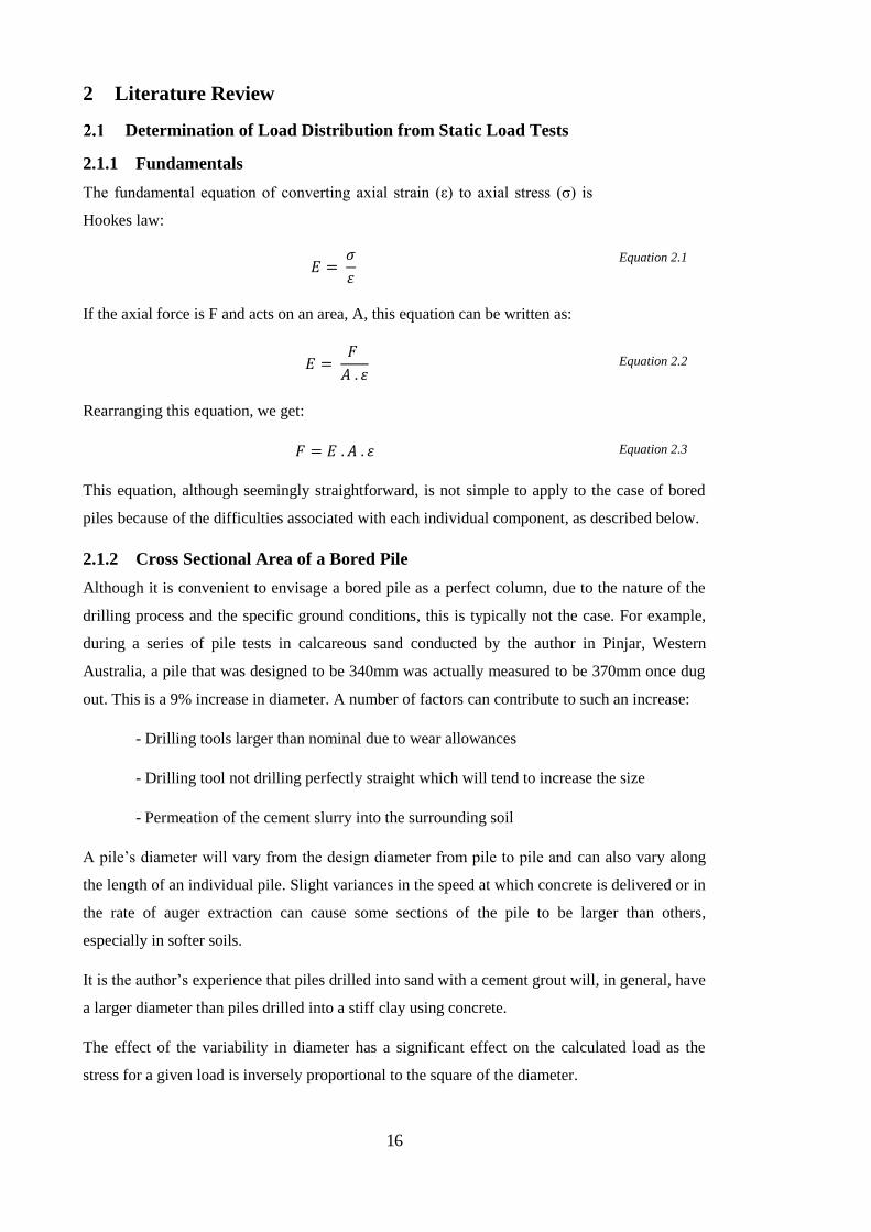
2.1.2 Cross Sectional Area of a Bored Pile
Although it is convenient to envisage a bored pile as a perfect column, due to the nature of the
drilling process and the specific ground conditions, this is typically not the case. For example,
during a series of pile tests in calcareous sand conducted by the author in Pinjar, Western
Australia, a pile that was designed to be 340mm was actually measured to be 370mm once dug
out. This is a 9% increase in diameter. A number of factors can contribute to such an increase:
- Drilling tools larger than nominal due to wear allowances
- Drilling tool not drilling perfectly straight which will tend to increase the size
- Permeation of the cement slurry into the surrounding soil
A pile’s diameter will vary from the design diameter from pile to pile and can also vary along
the length of an individual pile. Slight variances in the speed at which concrete is delivered or in
the rate of auger extraction can cause some sections of the pile to be larger than others,
especially in softer soils.
It is the author’s experience that piles drilled into sand with a cement grout will, in general, have
a larger diameter than piles drilled into a stiff clay using concrete.
The effect of the variability in diameter has a significant effect on the calculated load as the
stress for a given load is inversely proportional to the square of the diameter.
Equation 2.1
Equation 2.2
Equation 2.3

17
The cross-sectional area of a bored pile is a function of its Diameter:
𝐴 = 𝜋. 𝐷2
4
Inserting Equation 2.3a into Equation 2.3 and assuming E = 1, ɛ = 1 and varying D from 100%
Figure 2.1 is produced which shows the corresponding error in pile force that an error in the
assumed pile diameter would cause. As indicated by the Pinjar case history mentioned above, a
pile diameter 9% larger than nominal is possible and this would cause the calculated load to be
20% lower than actual. On the other hand, if the actual diameter was 95% of the design
diameter the calculated load would be 10% higher than actual.
It should also be noted that most methods of determining stress from strain assume a constant
diameter. This is not always the case with bored piles and this assumption can lead to apparent
variations in the modulus of elasticity at different depths. In a similar way to Figure 2.1, Figure
2.2 illustrates what an error in the diameter assumption can make to the calculation of the
modulus of elasticity (Ec). The Ec value has been chosen to have a nominal value of 35,000 MPa
for illustrative purposes. D and ɛ have been assumed constant at 1 and then Ec has been varied
Figure 2.1: Calculated load errors resulting from pile diameter variation
Figure 2.2: Illustration of effect of pile diameter on the apparent Modulus of Elasticity
Equation 2.3a

18
to show the resultant error in force. As can be seen, a typical error in the assumed diameter can
cause the apparent elastic modulus to vary over a range that is typically observed in concrete.
When applying the methods described later in this chapter, calculated changes in modulus
values are likely to indirectly include changes in cross sectional area.
It is clear that knowing the actual diameter or cross sectional area of a pile is fundamental in
analysing strain gauge data. It is however, practically impossible to accurately measure pile
dimensions. There are tools such as the Sonic Caliper test which can determine the actual
diameter for bored piles but the author knows of no current technologies to do this for CFA
piles. For CFA piles the top (exposed) diameter is generally assumed to continue down the rest
of the pile.
2.1.3 Modulus of Elasticity of Concrete / Grout
The modulus of elasticity determines the relationship between the stress and strain in concrete
and is fundamental in determining the stress at particular strain levels. In contrast to steel, for
which the modulus of elasticity is within a couple of percent of 200 GPa, the elastic modulus of
concrete / grout is not a fixed constant.
Concrete Ingredients
Concrete is a mixture of aggregates, cement and water. The aggregates and cement vary from
location to location due to the raw materials available. The variation in ingredients alone will
create variations in the specific properties. A broad range of mixes are used for piles, these
include; normal concrete, specially designed high slump concrete, sand grouts and cement
slurries. All of these mixes have different proportions of cement, aggregates and water and a
corresponding range of moduli should be expected.
The Australian Concrete Structures Standard AS3600 Clause 3.1.2 recommends the following
equations to estimate the modulus of elasticity of concrete (in MPa):
𝐸𝑐 = (𝜌1.5) . (0.043 . √𝑓𝑐𝑚𝑖 ) 𝑤ℎ𝑒𝑛 𝑓𝑐𝑚𝑖 ≤ 40 𝑀𝑃𝑎
𝐸𝑐 = (𝜌1.5) . (0.024 . √𝑓𝑐𝑚𝑖 + 0.12) 𝑤ℎ𝑒𝑛 𝑓𝑐𝑚𝑖 > 40 𝑀𝑃𝑎
Where ρ is the density of concrete, expressed in kg/m3 and
𝑓𝑐𝑚𝑖 is the mean in situ compressive strength (expressed in MPa), which is taken as 90% of the
cylinder tests mean
The Standard notes that “consideration should be given to the fact that this value has a range of
±20%”, this is reflective of the variable nature of concrete. Taking all the factors into account,
this level of accuracy isn’t surprising and is a large part of why there is difficulty converting
strain to load in concrete.
Equation 2.5
Equation 2.4

19
Non Linearity of Modulus
The modulus of elasticity for concrete is often assumed to be linear for simplicity but it is
known that it can be more accurately modelled using a quadratic function of strain.
Figure 2.3 shows a normalised stress strain curve for a local concrete supplied for pre cast piles
(Lehane et al 2003). This shows that the stress strain relationship is not linear. The linear
assumption is Ok for the working load ranges of piles. However, as the pile stress increases,
significant errors can be introduced depending on the value chosen for the slope of the linear
function. As it is reasonably simple to incorporate the non-linearity of concrete into
calculations, it should be done wherever possible to remove these errors.
Modulus of Neat Cement Grout
A neat cement grout is a mixture of cement, water and admixtures that typically increase fluidity
allowing lower w/c ratios. The absence of aggregates in these grouts leads to a lower modulus
of elasticity than concrete. These grouts are commonly used in micropiles and anchors so an
understanding of their Young’s moduli is clearly important. Hyett, Bawden and Coulson (1992)
studied the physical and mechanical properties of these grouts including the modulus of
elasticity. Figure 2.4 shows a plot they produced comparing the Young’s modulus to the water
cement ratio. It is evident that the Young’s modulus is substantially lower than that of concrete
and sand cement grouts that are used on larger CFA piles. There is strong correlation between
the w/c ratio and the Young’s modulus. Typical grouts used for micropiles and anchors will
have a w/c ratio of between 0.4 and 0.5 which suggests that the Young’s modulus of these
grouts should be in the 9 GPa to 13 GPa range.
Figure 2.3: Non-Linear stress vs normalised strain for local concrete specimen
--- Linear with σ/f’c = 0.2
--- Linear with σ/f’c = 0.4
--- Test Data
---

20
Concrete creep under load
Creep is the increase in strain under a constant load. It is independent of shrinkage or swelling
effects and is known to be greater in young concrete specimens. Piles that undergo a load test
are typically loaded within 2 weeks which would be considered at the early stages of the
concrete’s age so the creep effects will affect the development of strain in the pile.
The best way to isolate the creep effects is to load the pile at a constant rate. This means no load
holds or unloading loops. These holds and loops are almost always specified in pile load test
specifications so a decision needs to be made about what the pile test is aiming to achieve; a
more accurate measurement of the soil/pile behaviour or confirmation of the pile’s suitability to
the working loads.
2.1.4 Measuring Strain
Strain is a measurement of the relative expansion or contraction of a material. Strain is
essentially a measurement of displacement and there are two primary ways of measuring this in
piles:
- Tell-tale rods
- Embedded strain gauges
Tell-tales
Tell tales are stiff rods that are anchored at a certain point in a pile and de-bonded above this
point. They measure relative movement of this point in the pile against the pile head. These
have not been used in any of the cases studied (and usually only employed in Osterberg Cell
tests) and are therefore not considered in detail in this chapter.
Figure 2.4: Young’s Modulus vs w/c ratio for neat cement grouts (Hyett et al. 1992)

21
Strain gauges
Strain gauges take many forms but are fundamentally a sensor that measures the change in
displacement over a small length and then converts this into a signal for recording. Typically,
vibrating wire or electrical resistance strain gauges are used whilst the relatively newer fibre
optic technology has shown some potential. The National Instruments white paper FBG Optical
Sensing: A New Alternative for Challenging Strain Measurements (2016) provides a concise
description about each type of gauge and their advantages and limitations.
As with many aspects of the foundation industry, data logging systems can be expensive and
tend to be specifically designed for certain types of sensors, i.e. vibrating wire gauges will not
work on a system set up for electrical resistance gauges. This fact means that the type of gauge
used in a pile test can be more a function of what logging systems are available rather than the
best type of strain gauge for the test.
For the tests analysed in the following sections, electrical resistance strain gauge sister bars have
been used. Geokon 3911A sister bars (Figure 2.5) as well as sister bars manufactured by CMR
Tech (a local company in Perth, Western Australia) have been used in these studies. It is noted
that there has been a preference by piling engineers to use vibrating wire strain gauges. Their
robustness and reliability have been named as reasons for this. Common criticism of electrical
resistance strain gauges are that the long cables can distort the signal and they don’t last as long
as vibrating wire gauges over long periods. No significant issues are considered likely in this
study as the piles examined are short (<20m) and these are not monitored for long term
performance.
Geometrical Compatibility
An issue at the centre of using strain gauges for bored piles is the question of whether the strain
in the steel equals the strain in the concrete. Lam and Jeffries (2011) examined this in some
detail and came to the conclusion that this assumption appears reasonable as long as well-
designed strain gauges (with sufficient anchorage lengths either side of the strain measuring
Figure 2.5: Geokon 3911A Strain Gauge Sister bars

22
location) are used. This is consistent with general industry consensus and the widespread use of
embedment strain gauges and sister bars.
Strain Averaging
It is very common practice to install two or more strain gauges at each level spaced evenly
around the cage. This is to account for bending effects in the pile which will cause uneven
distribution of the axial load stress and, if only one strain gauge is used and is placed in the
wrong location, readings can be misleading. The measurement of dissimilar strains at a given
pile level can raise concerns about the reliability of the strain gauge outputs. As bending
moments are generally only significant in the upper few pile diameters, significantly dissimilar
strains at any given level below the upper pile section should not arise due to the application of
axial load.
Temperature Effects
Even when designed to compensate for temperature effects strain gauges can be sensitive to
temperature. This is due to two primary reasons:
- Thermal expansion of the gauge and/or the surrounding materials.
- Thermal effects in the strain measuring system. For example, a change in electrical
resistance in the system cables that will affect the raw voltage reading.
Assuming pile tests are conducted once the concrete/grout has sufficiently cured (i.e. dissipated
the majority of the heat created by the cement hydration), there would be very little change in
temperature in the gauges throughout the test as they are embedded in concrete which has high
insulation properties. Temperature effects would therefore be of little concern during a pile test
unless the test is on early age concrete and conducted over a long duration (>24 hours).
However, if the pile strains are monitored throughout curing to examine possible residual loads,
then the temperature effects are of great importance.
Other Possible Sources of Error
Even when perfectly manufactured gauges can still malfunction, other possible sources of error
or malfunction can be:
- Damaged or severed cable(s)
- Gauge not vertical in pile
- Pile cage not central, or possibly touching side of hole
- Defects in pile shaft
23
Once a pile is cast it is practically impossible to check for most of these errors so care must be
taken in the installation.
Logging Devices
There are a large number of logging devices available and it is beyond the scope of this thesis to
discuss different types. However, during one of the tests the author was involved with, the
logger malfunctioned and all the electronic data were lost. Luckily the load displacement data
were recorded manually at critical points throughout the test; no strain gauge data were recorded
manually which is a valuable lesson for anyone conducting load tests.
2.1.5 Methods of converting strain to load
The methods that have been used to convert strain to load are essentially Modulus of Elasticity
calculations as the cross sectional area is almost always assumed to be constant. However, it
needs to be remembered that, although the Modulus of Elasticity is being derived or calculated,
there will almost definitely be an error contribution from variations in pile cross sectional area.
In this chapter, the methods will only be briefly described. For more in depth descriptions of
each method, the reader should consult the literature and the paper by Lam and Jeffries (2011).
Figure 2.8 is an extract from this paper and provides a useful summary of the methods
examined.
Transformed Area Method
This method is a calculation of the modulus by looking at the proportion of steel and concrete in
the cross section. It relies on how the concrete’s modulus (Ec) is determined e.g. from historical
data, cylinder tests or cores direct from the pile. The combined axial rigidity can be described
as:
𝐸𝑃𝐴𝑃 = 𝐸𝑐 . 𝐴𝑐 + 𝐸𝑠 . 𝐴𝑠
Uncorrected Area Method
This method is a simplified version of the transformed area method in which only the area and
modulus of the concrete is considered:
𝐸𝑃 = 𝐸𝑐
The uncorrected area method and transformed area method are the least accurate methods as
they don’t utilise actual strain gauge readings to calculate the modulus. However, when strain
gauges have not been placed near the pile head, pile designers have little choice but to use these
equations.
Equation 2.6
Equation 2.7

24
It should also be considered that these methods provide a benchmark that other methods can be
compared against. Methods that calculate modulus values that significantly vary from those
used in the uncorrected and transformed area method should be treated with caution.
Dummy Pile Method
This method involves creating a pile model and testing it in the laboratory to measure the
modulus. Although significantly better than the two previously described methods, it will miss
variations in the pile and in situ effects that can modify the modulus and area values.
Implicit Method
This method is based on the assumption that the load at any point is simply the ratio of the strain
at that point to the strain at the pile head multiplied by the load at the pile
head:
𝑃𝑖 = 𝑃1 . (휀𝑖
휀1)
where Pi = Load at location i, P1 = load at top strain gauge, εi = strain at location i, ε1 = strain at
top strain gauge
This method also assumes that, at a given head load, the EA of the pile is constant throughout.
This method may also be extended to when the cross sectional area of the pile is known at
different levels by introducing A1 and Ai to the above equation.
Linearly Elastic Method
As the name suggests this method assumes a constant E value which is calculated from the
strain gauge at the top of the pile and then applied to the remainder of the strain
gauges.
𝐸 =∆𝑃
𝐴∆𝜀
Secant Modulus Method
This method allows the modulus to be varied in accordance with the strain reading at that gauge.
This method takes into account the non-linearity of the stress strain curve. To apply this method,
the stress strain curve at the uppermost gauge level is plotted and then a line of best fit is applied
to this typically in the form:
𝐸 = 𝑎 . 휀 + 𝑏
Where a and b are constants from the line of best fit.
Equation 2.8
Equation 2.9
Equation 2.10

25
Tangent Modulus
This method, as described by Fellenius (2001), is more involved than methods described above
and relies on the relatively high stiffness of pile shaft friction when a pile is loaded. As shown in
Figure 2.6 the displacement curve for shaft friction is typically assumed to reach peak stress by
1% of diameter and does not change thereafter. By comparing the change in stress to the change
in strain after the maximum shaft stress is reached, a ‘calibrated’ EA value can be derived for
each strain gauge level.
The equations for this method are as follows:
𝜎 = 𝑎휀2 + 𝑏휀
𝐸𝑡 = 𝑑𝜎
𝑑휀= 𝑎휀 + 𝑏
𝐸 = 0.5𝑎휀 + 𝑏
Where Et is the Tangent Modulus, E is the Secant Modulus
As these equations get applied at each gauge level this calibrated value should allow for changes
in the cross sectional area of the pile as well as variations in the modulus of the concrete but
cannot distinguish the contribution of each of them. This method should lead to more accurate
calculations of the pile load distribution.
As noted by Lam and Jeffries (2011) this method would only work for piles with significant pile
movement. It will be difficult to apply to piles tested to working load only.
As mentioned by Fellenius, to obtain the most reliable results, a pile should be loaded at a
continuous rate as creep holds and unload reload loops cause strains without extra load,
distorting the calculations.
Figure 2.6: Typical normalised shaft friction vs displacement curves (Reece and Oneil 1988)
Equation 2.11
Equation 2.13
Equation 2.12
26
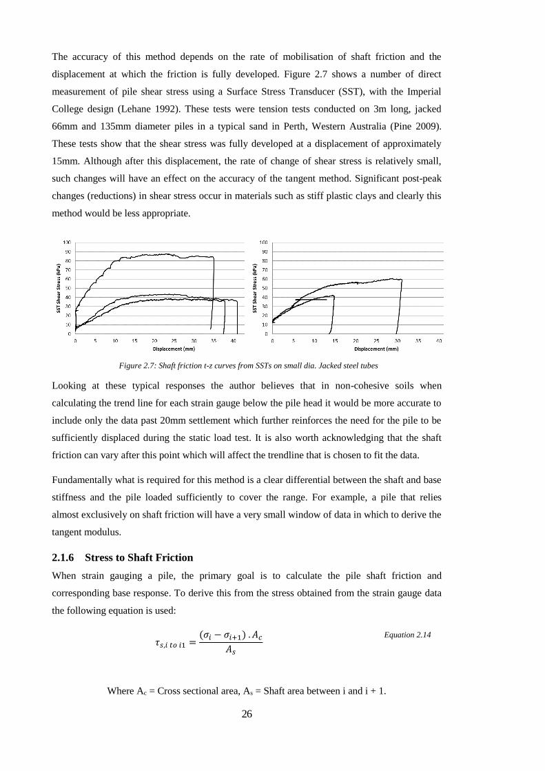
The accuracy of this method depends on the rate of mobilisation of shaft friction and the
displacement at which the friction is fully developed. Figure 2.7 shows a number of direct
measurement of pile shear stress using a Surface Stress Transducer (SST), with the Imperial
College design (Lehane 1992). These tests were tension tests conducted on 3m long, jacked
66mm and 135mm diameter piles in a typical sand in Perth, Western Australia (Pine 2009).
These tests show that the shear stress was fully developed at a displacement of approximately
15mm. Although after this displacement, the rate of change of shear stress is relatively small,
such changes will have an effect on the accuracy of the tangent method. Significant post-peak
changes (reductions) in shear stress occur in materials such as stiff plastic clays and clearly this
method would be less appropriate.
Looking at these typical responses the author believes that in non-cohesive soils when
calculating the trend line for each strain gauge below the pile head it would be more accurate to
include only the data past 20mm settlement which further reinforces the need for the pile to be
sufficiently displaced during the static load test. It is also worth acknowledging that the shaft
friction can vary after this point which will affect the trendline that is chosen to fit the data.
Fundamentally what is required for this method is a clear differential between the shaft and base
stiffness and the pile loaded sufficiently to cover the range. For example, a pile that relies
almost exclusively on shaft friction will have a very small window of data in which to derive the
tangent modulus.
2.1.6 Stress to Shaft Friction
When strain gauging a pile, the primary goal is to calculate the pile shaft friction and
corresponding base response. To derive this from the stress obtained from the strain gauge data
the following equation is used:
𝜏𝑠,𝑖 𝑡𝑜 𝑖1 =(𝜎𝑖 − 𝜎𝑖+1) . 𝐴𝑐
𝐴𝑠
Where Ac = Cross sectional area, As = Shaft area between i and i + 1.
Figure 2.7: Shaft friction t-z curves from SSTs on small dia. Jacked steel tubes
Equation 2.14

27
Fig
ure
2.8
: Su
mm
ary
of
Ana
lysi
s M
eth
od
s fr
om
La
m (
201
1)

28
Parameter Selection for Bored Piles in Sand
2.2.1 Pile Capacity Fundamentals
Static pile capacity calculations begin with Equation 2.15 which states that the pile total
capacity (Qt) is the sum of its base capacity (Qb) and its shaft capacity (Qs):
𝑄𝑡 = 𝑄𝑠 + 𝑄𝑏
Base Capacity (Qb)
A pile’s base capacity is typically defined as the force needed to cause a displacement of 10% of
the pile’s diameter and is represented by Equation 2.16:
𝑄𝑏 = 𝐴𝑏 . 𝑞𝑏0.1
Where Ab is the Area of a pile’s base and qb0.1 is the pressure at a displacement of 10% D
Shaft Capacity (Qs)
A pile’s shaft capacity is defined by Equation 2.17:
𝑄𝑠 = 𝐴𝑠 . 𝜏𝑓
Where As is the shaft area and τf is the shaft friction at failure
The shaft friction developed at failure is then expanded into the following
equations:
𝜏𝑓 = 𝜎′ℎ𝑓 . tan 𝛿
𝜎′ℎ𝑓 = 𝜎′ℎ0 + ∆𝜎′ℎ𝑐 + ∆𝜎′ℎ𝑑
Where: σ’hf is the horizontal effective stress at failure
σ’h0 is the initial horizontal effective stress
δ is the interface friction angle between the soil and the pile
Δσ’hc is the change in horizontal effective stress due to construction effects
Δσ’hd is the change in horizontal effective stress during shearing at the pile soil interface
(dilation)
These inputs and their relationship to CPTs will be discussed later in this section.
Equation 2.15
Equation 2.16
Equation 2.17
Equation 2.19
Equation 2.18

29
2.2.2 Pile Deformation Fundamentals
How a soil and pile responds to a load applied at the pile’s head is incredibly complex. As such
it is practically impossible to represent this completely by a set of equations. But in its basic
form a pile’s response can be described as the combination of three components:
1. The axial compression of the piles
2. Shear response of the pile’s shaft
3. The base response
Fleming et al. (1985) describes the basic solution for the deformation of a pile and splits it into
the above three components.
Axial Compression
This is the simplest of the components to evaluate as the Young’s Modulus of concrete and steel
are many times more certain than soil properties. The axial strain at any level down the pile is
defined by Equation 2.20:
휀𝑧 = −𝑑𝑤
𝑑𝑧=
𝑃
𝜋. 𝑟02. 𝐸𝑝
Where P is the axial load at that point, r0 is the pile radius and Ep is the Young’s Modulus of the
pile. Despite the Young’s modulus of concrete being shown to be non-linear, for simplicity, the
Young’s modulus of concrete in these equations will be assumed to be constant as the
uncertainty in soil parameters will far outweigh the error introduced by a constant Young’s
modulus.
Pile Shaft
Fleming et al. explains the deformation of a pile shaft in soil by considering the pile surrounded
by concentric cylinders of soil with shear stresses on the interface between each cylinder.
Vertical equilibrium requires that each cylinder will have the same total force as the cylinder
inside of it. As the area of the cylinders will increase linearly with their radius (r) then the shear
stress at any given cylinder can be represented by:
𝜏 =𝜏0𝑟0
𝑟
Where τ0 is the shear stress at the pile soil interface and r0 is the pile radius.
Equation 2.20
Equation 2.21

30
Fleming et al. (1985) describes the mode of deformation around a pile as primarily one of shear
therefore it is more natural to develop the solution in terms of shear modulus (G) and Poisson’s
ratio ν. Noting that the shear modulus may be related to the Young’s modulus by:
𝐺 =𝐸
2. (1 + 𝑣)
The shear strain (y) in the soil is given by:
𝑦 = 𝜏
𝐺
Since the main deformation in the soil will be vertical the shear strain will approximately equal:
𝑦 ≅ 𝑑𝑤
𝑑𝑟
Where w is the vertical deformation.
The total vertical deflection of the pile is therefore the sum of all the shear strains in the soil
mass (imagined as concentric cylinders sliding against each other). This can be calculated by
integrating the combination of the above equations which gives the following:
𝑤 = ∫𝜏0𝑟0
𝐺. 𝑟𝑑𝑟 =
𝜏0𝑟0
𝐺
𝑟𝑚
𝑟
ln(𝑟𝑚
𝑟⁄ )
Where rm is the maximum radius at which deflections in the soil are assumed to become
insignificant.
Randolph and Wroth (1978) empirically found this radius to be of the order of the length of the
pile. Typical pile dimensions lead to the value of ln(rm/r) to be between 3 and 5 averaging 4
(Baguelin and Frank 1979). Due to this small range ln(rm/r) it is typically represented by ζ.
Pile Base
The pile base can be treated as a bearing capacity problem therefore the standard settlement
solution equation can be used. Substituting in G, rb (radius of pile base) and Pb (Pile base load)
Timoshenko and Goodier (1970) showed that this can be written as:
𝑤𝑏 = 𝑃𝑏(1 − v)
𝑟𝑏𝐺𝑏 . 4
Overall
Combining these three components will give the solution to the pile’s displacement under a
given load. However, it is not that simple.
The main problem with the above equations is that the primary input, the shear modulus (G), is
difficult to derive from in situ tests and is not a constant value as shown further on it reduces
with increasing stress. Applied to the shaft stress equation above this means that as the shear
stress decreases away from the pile the shear modulus will be increasing. This results in a
unique value of G for every point between r0 to rm. Not only this but each point will then vary
Equation 2.22
Equation 2.23
Equation 2.24
Equation 2.25
Equation 2.26
31
with each change in shear stress. This makes solving Equation 2.25 extremely difficult, even
with the correct inputs this will require significant computational effort.
The difficulty in solving these problems is well documented and a number of computer
programs have been developed to assist in solving these. The program RATZ created by
Randolph is one of these programs and is commonly used to determine a pile’s load
deformation curve.
2.2.3 RATZ
RATZ is a Microsoft Excel based computer program that is designed to analyse a pile’s axial
load transfer. Its analysis uses the equations described above combined with load transfer curves
of the soil around and below the pile to produce a t-z curve for the pile. It utilises the explicit
time based approach (Cundall and Stack 1979) which avoids the need for large amounts of
computational power (ie Plaxis).
The program has three main inputs in line with the above equations:
1. Pile Structural parameters
2. Shaft Friction parameters
3. Pile Base parameters
Pile Structural Parameters
These parameters are straightforward and include pile dimensions and material properties. It is
sufficiently flexible so that piles of varying properties can be inputted (ie enlarged bases, hollow
etc)
Shaft friction Parameters
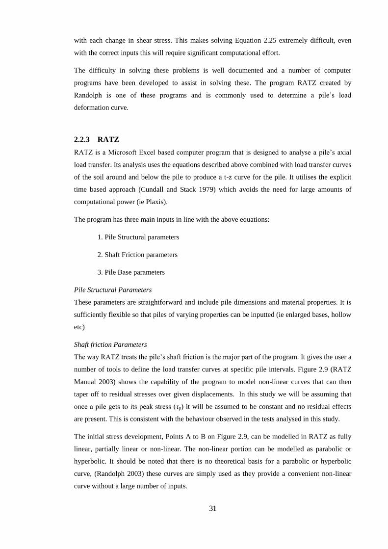
The way RATZ treats the pile’s shaft friction is the major part of the program. It gives the user a
number of tools to define the load transfer curves at specific pile intervals. Figure 2.9 (RATZ
Manual 2003) shows the capability of the program to model non-linear curves that can then
taper off to residual stresses over given displacements. In this study we will be assuming that
once a pile gets to its peak stress (τp) it will be assumed to be constant and no residual effects
are present. This is consistent with the behaviour observed in the tests analysed in this study.
The initial stress development, Points A to B on Figure 2.9, can be modelled in RATZ as fully
linear, partially linear or non-linear. The non-linear portion can be modelled as parabolic or
hyperbolic. It should be noted that there is no theoretical basis for a parabolic or hyperbolic
curve, (Randolph 2003) these curves are simply used as they provide a convenient non-linear
curve without a large number of inputs.
32
In order to determine the non-linear load transfer curve the program requires the following
inputs:
1. Shear modulus (G) at each pile segment, noting G is a program specific value that
can be determined from back analysing load tests
2. Load transfer parameter (ζ) as described previously represents at what distance the
shear strains are negligible
3. Peak shaft friction (τp)
4. Yield threshold (ξ). This determines how large the linear part of the curve is, if ξ=1
then the shaft stress is fully linear
Given these inputs it can be shown that there is only one parabolic or hyperbolic solution to the
non-linear part of the curve.
Pile Base Response
Similar to the pile shaft the program models the base response as either parabolic or hyperbolic.
Again there is no theoretical reason for this, it simply provides a conveniently solved non-linear
curve. Given a specified base pressure at a given movement the program uses the pile base
bearing capacity equation above (EQ 2.26) to derive an initial slope and then derive a curve.
Figure 2.9: RATZ shaft load transfer curve

33
RATZ is a useful program as it provides a convenient way to model the non-linear behaviour of
piles. Its relative simplicity comes from a number of simplifications that although have no
theoretical basis are necessary to model non-linear effects without making the program too
complicated. As such when using the program to match load testing data, a ‘perfect fit’ should
not be expected. Due to the large number of variables models that closely match test data can be
produced however care must be taken that these matches aren’t produced using parameters that
are outside established ranges or supported by other evidence.
2.2.4 Cone Penetrometer Test
When studying the correlation between the results of a CPT and a pile’s behaviour it is
fundamental to understand what a CPT is and what factors influence its results. A greater
understanding about what affects a CPT will lead to improved logic being applied to
correlations with pile design parameters.
Description of Test and Instrument
Introduced in its current form in about 1932 in the Netherlands the CPT is described by Lunne
(1997):
In the Cone Penetration Test (CPT), a cone on the end of a series of rods is pushed into the
ground at a constant rate and continuous or intermittent measurements are made of the
resistance to penetration of the cone. Measurements are also made of either the combined
resistance to penetration and the outer surface of a sleeve or the resistance of a surface sleeve.
Figure 2.10 shows a typical cone. Although many different cones are available, current industry
practise is to use Electrical Friction Cone Penetrometers almost exclusively. The International
Test Procedure ISSMFE 1989 has been established as the reference procedure for CPT tests.
This defines the following primary characteristics of the reference test:
- A cone of diameter 35.7mm and angle 60o (Area of cone (Ac) = 1,000 mm2)
- A friction sleeve of length 133.7mm and diameter 35.7mm (Sleeve Area (As) = 15,000mm2)
- Penetrated into the ground at a constant rate of 20mm/s

34
In Australia AS 1289.6.5.1 – 1999 governs the method however it is largely in line with the
International Test Procedure.
Compared to other soil investigation methods CPTs are lower cost, typically more repeatable
and provide a detailed soil stratigraphy profile. In addition to this there are obvious similarities
to how a CPT is conducted to how a pile is loaded. This has led to it becoming a popular soil
investigation method that pile performance can be related to. However, it does have some
drawbacks; in its standard form a CPT does not return physical samples back to the surface for
identification, it requires a large reaction force which limits its depth in dense soils and has
difficulty penetrating cemented materials.
Factors Affecting CPT Results in Coarse Grained Materials
Calibration chamber testing has shown that the cone resistance is controlled by sand density, in
situ vertical and horizontal effective stress and sand compressibility (Lunne 1997).
Figure 2.10:Typical CPT Cone

35
Sand Density
Typically described as the relative density (Dr) which is defined by Equation
2.27:
𝐷𝑟 = 𝑒𝑚𝑎𝑥 − 𝑒
𝑒𝑚𝑎𝑥 − 𝑒𝑚𝑖𝑛
Where e is the in situ void ratio and emin and emax are the soil’s minimum and maximum void
ratios as determined by laboratory methods.
Dr is important as it is commonly used to estimate a sand’s peak friction angle (φ’p). φ’p is the
upper limit of the interface friction angle above in Equation 2.18 (δ). φ’p is also a significant
factor in the equations that govern qb,0.1.
Baldi et al (1986) conducted an extensive calibration chamber testing and proposed the
following relationship between qc, σ’v0 and Dr.
𝐷𝑟 = 1
𝐶2 ln (
𝑞𝑐
𝐶0 . (𝜎′𝑣0)𝐶1 .
)
Where C0, C1 and C2 are soil constants. See Figure 2.11 for the curves produced using their
suggested constants.
Overall Lunne (1997) states that there is a high to moderate reliability of deriving Dr from a
CPT test which is why it has been typically used as an intermediate parameter.
Figure 2.11:CPT qc relationship to Dr (Baldi et al 1988)
Equation 2.27
Equation 2.28
36
Horizontal effective stress (𝜎′ℎ0)
The in situ horizontal stress is often represented by:
𝜎′ℎ0 = 𝐾0 . 𝜎′𝑣0
For normally consolidated soils K0 can be approximately related to the soils friction angle
however, in over consolidated soils it depends on the stress history of the soil and will have
significant variation.
It is an important parameter used in nearly all soil mechanics problems however it has
historically been a very difficult measurement to make with any device and such measurements
are usually unreliable (Lunne 1997). Although tests have shown that 𝜎′ℎ0 makes a significant
contribution to CPT results there are no reliable methods for determining 𝜎′ℎ0 from CPT results.
2.2.5 Shaft Friction at Failure Correlations
As described in Eq 2.19 the shaft friction is a factor of σ’h0, δ, Δσ’hc and Δσ’hd. σ’h0 has been
shown to have a significant effect on CPT tip resistances. Dr has also been shown to affect CPT
results and is also a large factor in determining δ. This is why correlation between a CPT test
and the shaft friction at failure on a pile is expected.
Because of this there has been a lot of effort into correlating CPT qc to shaft resistance through
the use of βc, defined as:
𝜏𝑓 = 𝑞𝑐
𝛽𝑐
However there has been no definitive answers with a wide range of βc values proposed. This
variation is best represented by the plot produced by De Cock et al. (2003) Figure 2.12 which
shows the various predicted shaft frictions for different countries in Europe.
Lehane (2009, 2012) conducted a study into the relationship between CPT qc and shaft friction
in Perth sands and found that the effects of dilation have a significant influence on this
relationship. There are important dilation effects at the pile soil interface which are dependent
on pile diameter and can increase Δσ’hf significantly (and hence reduce βc). He did note that the
βc values in his study ranged from 125 to 250 and averaged 175 which is the range and average
that appear in other studies.
Equation 2.29
Equation 2.30

37
2.2.6 Shear Modulus of Sand (G)
The Shear Modulus determines the relationship between shear stress (τ) and shear strain (γ), i.e..
𝐺 = 𝜏
𝛾
As seen in the pile deformation equations it is a fundamental parameter required to solve them.
As mentioned previously G is not linear and decreases from an initial value G0 as the shear
stress increases. Figure 2.13 shows the results from self-boring pressure meter tests conducted at
a site in Perth (Fahey 2007). This shows how the pressure and strain readings from the device
are varying. Although not a direct plot of shear stress vs shear strain, it is closely related and
shows the general non-linear nature of the shear modulus.
Due to the difficulty in obtaining undisturbed samples of cohesionless soils, in situ
measurements of G are preferred. Plate load tests can be used for shallow foundations however
the pressuremeter is the only real option of obtaining direct in situ measurements of G.
Unfortunately, pressuremeter testing is difficult and expensive so is not widely used in practise.
This is why correlating G to other in situ tests is necessary.
Past studies have related G0, E0 and Eequiv to 𝐶 √𝑞𝑐 . 𝜎′𝑣 . 𝑝𝑎𝑡𝑚3
(Robertson 1997, Baldi 1989,
Fahey 2003) where C is a constant depending on a number of factors including strain level.
These studies have had C ranging by a factor of 4 even assuming a constant strain which is
showing that the relationship between qc and stiffness is not that reliable.
Figure 2.12: CPT qc relationship to pile shaft friction (De Cock)
Equation 2.31

38
In addition to this nearly all the studies examine the soil stiffness in relation to a certain strain
level. When attempting to estimate a pile’s t-z curve the full range of strain levels are
experienced and an understanding of the change in soil modulus is needed however is
practically impossible to confidently predict this.
2.2.7 Pile Base Capacity
Bored piles in coarse grained soils will only experience a plunging type failure when the pile
has been displaced a distance of approximately one base diameter. A typical structure would
have failed far before movements of this magnitude are achieved; ie a 450mm pile that has
moved 450mm will have dire consequences for the structure it’s supporting. Because of this it
has been convention to determine a pile’s ultimate capacity when it has reached a displacement
of 10% of the diameter (qB,0.1D). As such determining the capacity of a bored pile in sand is
more a question of the soil’s stiffness rather than its true bearing capacity.
Past studies have correlated qB,0.1D directly to qc by Equation 4.18:
𝑞𝐵,0.1𝐷 = 𝑞𝑏 . 𝛼𝑏
Where qb is an appropriately averaged CPT tip resistance at the base and αb is a constant
Figure 2.13: Self Boring Pressuremeter Test results at a Perth Sand Site (Fahey 2007)
Equation 2.32

39
These studies generally suggest using an αb value of between 0.15 and 0.20 however some
recommend values up to and exceeding 0.5. Based on previous correlations on soil stiffness and
a database of bored piles in sand and numerical predictions by Lee & Salgado (1999), Lehane
(2009) proposed that qB,0.1D take the form
𝑞𝐵,0.1𝐷 = (2.4 ± 0.7). 𝑞𝑐 0.5 . 𝜎𝑣0
′ 0.25 . 𝑝𝐴𝑇𝑀 0.25
Equation 2.33

40
Chapter 3
Test Sites

41
3 Test Sites
This chapter describes the location, ground conditions, test details and results of the test sites
examined in this study. Five tests have been examined in this study; 500 Hay St Subiaco, 999
Hay St Perth, Cockburn Gateway Shopping Centre, Cloisters Redevelopment Perth and the
UWA IOMRC Crawley. These sites are identified on Figure 3.1 which shows their location in
the Perth Metropolitan Region. Geotech information is typically CPTs which will be plotted for
each test.
UWA IOMRC Crawley
500 Hay St Subiaco
Cloisters Redevelopment Perth
999 Hay St Perth
Cockburn Gateway Shopping Centre
Figure 3.1: Location of Test Sites in the Perth Metropolitan region

42
500 Hay St Subiaco
3.1.1 Location
This test site is located at 500 Hay St Subiaco approximately 3km west of the Perth CBD. The
site has an area of approximately 4,000 m2 and will comprise of a 3 level basement with a 6
level office occupying half the site above ground and a 10 storey hotel and cinema occupying
the remainder. The majority of the site was originally a cinema complex with a single level
underground carpark which has been demolished.
Figure 3.2 shows a general layout of the Northern portion of the site and a more detailed plan of
the test pile location is shown in Figure 3.3. The test piles were installed from the new B1 level
which was at an RL of 15.7m which is approximately 5.0m below existing ground level and
3.0m below the previous B1 level. The test pile location was determined by the project schedule
as it was a high priority and that area of site was available first.
Alv
an
St
North
Figure 3.2: 500 Hay St Test Area Location

43
3.1.2 Ground Conditions
The site is underlain by sand derived from Tamala Limestone. Due to the site’s size a large
number of CPTs were conducted however there are 4 CPTs in close vicinity to the test:
- CPT 14 was part of the original soils investigation and was conducted from the
original ground level (~5m above pile install). To account for the removal of
overburden pressure a correction was applied using a calibrated version of Equation
2.28. The CPTs on this site were conducted at various excavation depths which were
then compared to the values predicted using Equation 2.28. The constants in Equation
2.28 were then adjusted to provide a better fit. In this case C0 = 205, C1 = 0.53 and C2 =
2.93 were used. The corrected qc values are used in the plots.
-CPT 1, CPT 2 and CPT 2a were conducted after the load test from the pile install level.
CPT 1 and 2 refused at the pile base level however CPT 2a penetrated past the base but
is the furthest away from the test pile.
Figure 3.4 shows the tip resistance and friction ratio for the four CPTs. The tip resistance is very
consistent along the shaft however the base shows a large degree of variability which won’t
affect the strain gauge analysis in Chapter 4 however makes the parameter selection in Chapter
5 difficult. The water table was observed 9.0m below pile install level at an RL of 6.7m. It is
noted there is a consistent change in the friction ratio at this depth.
Figure 3.3: 500 Hay St Test Area Detailed Layout

44
Test Pile Details
The test pile on this site was a 600mm dia. 15.4m long CFA pile. Table 3.1 summarises the pile
details. The pile was instrumented with two types of strain gauges. Geokon 3911A Electrical
Resistance Sister Bars were placed in pairs at depths of 0.5m, 6.0m and 13.5m. These were at
the critical depths: 0.5m being the head value, 6.0m the final basement level and 13.5m near the
pile tip. Two pairs of strain gauges made by a local company CMR Technologies were also used
and place at levels of 3.0m and 10.0m. Ideally the base pair would have been a bit closer to the
toe but there were a number of reasons why they were higher:
1) For piles this deep the contractor tapers the bottom of the cage to assist with insertion. As the
gauges need to be as vertical as possible this meant they had to be placed above the taper.
2) The operator drilled the pile 400mm deeper than was planned.
All strain gauges were equipped with thermistors to monitor the pile temperature during curing.
Figure 3.4: 500 Hay St Subiaco Test Pile CPTs
Ele
vat
ion
(m
)
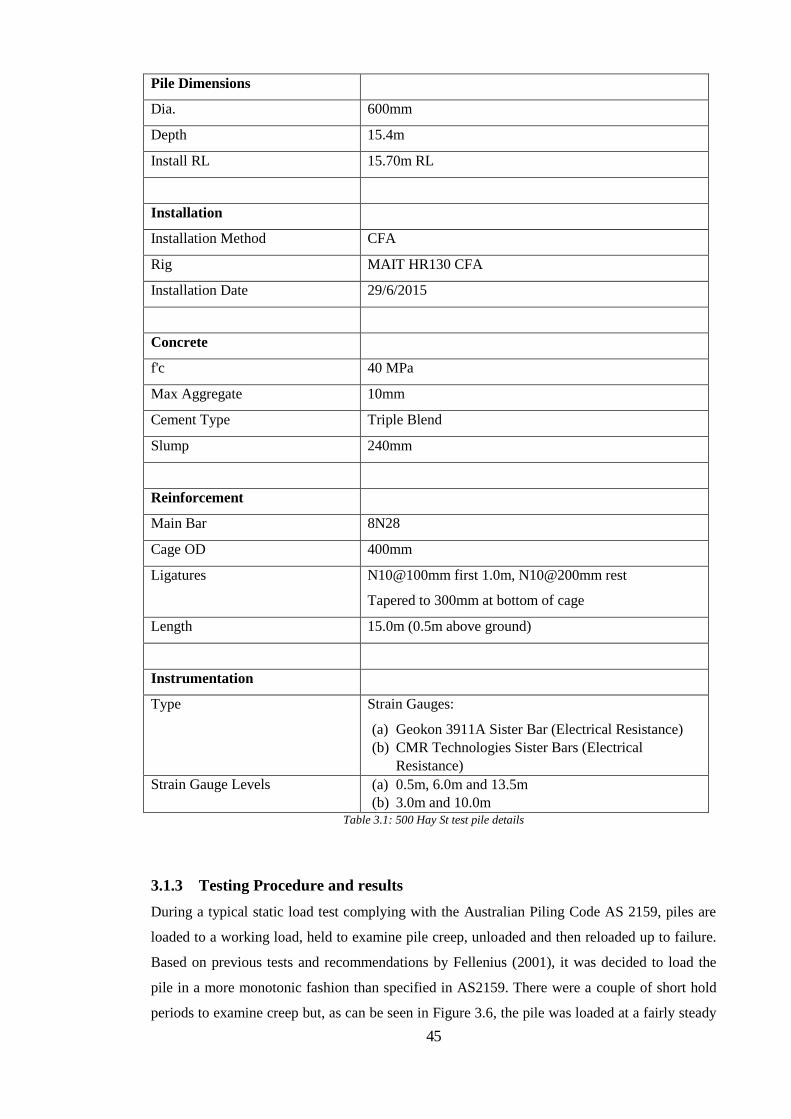
45
Pile Dimensions
Dia. 600mm
Depth 15.4m
Install RL 15.70m RL
Installation
Installation Method CFA
Rig MAIT HR130 CFA
Installation Date 29/6/2015
Concrete
f'c 40 MPa
Max Aggregate 10mm
Cement Type Triple Blend
Slump 240mm
Reinforcement
Main Bar 8N28
Cage OD 400mm
Ligatures N10@100mm first 1.0m, N10@200mm rest
Tapered to 300mm at bottom of cage
Length 15.0m (0.5m above ground)
Instrumentation
Type Strain Gauges:
(a) Geokon 3911A Sister Bar (Electrical Resistance)
(b) CMR Technologies Sister Bars (Electrical
Resistance)
Strain Gauge Levels (a) 0.5m, 6.0m and 13.5m
(b) 3.0m and 10.0m Table 3.1: 500 Hay St test pile details
3.1.3 Testing Procedure and results
During a typical static load test complying with the Australian Piling Code AS 2159, piles are
loaded to a working load, held to examine pile creep, unloaded and then reloaded up to failure.
Based on previous tests and recommendations by Fellenius (2001), it was decided to load the
pile in a more monotonic fashion than specified in AS2159. There were a couple of short hold
periods to examine creep but, as can be seen in Figure 3.6, the pile was loaded at a fairly steady

46
average rate of about 750kN per hour. There were a number of un-planned hold periods towards
failure which arose due to technical difficulties with the logging system.
Figure 3.5 shows the test pile setup. Reaction was provided by a series of test beams restrained
by tension piles. Load was applied using 6 x 100t hydraulic cylinders. Load was measured by a
load cell and displacement was measured at four points using displacement transducers attached
to reference beams. The hydraulic cylinders were controlled by a specially coded computer
program that also logs all the data. An advantage of the computer system is that the pile can be
loaded continuously as seen in Figure 3.6 and not with the typical stepped load seen in other
tests.
The measured pile load-displacement curve is shown on Figure 3.7, where it can be seen that the
pile reached an ultimate geotechnical load (RUG) of 4,664 kN, defined as the load at 10% of the
pile diameter (60mm). It can be seen that the load is still increasing at this point and a plunging
type failure has not occurred. This response is typical of a bored pile in sand, for which
additional resistance is developed up to pile displacements of about one pile diameter.
Figure 3.5: 500 Hay St Pile Test Setup

47
Figure 3.6: 500 Hay St Test Loading Schedule
Figure 3.7: 500 Hay Sy Load Test Load vs Displacement Curve
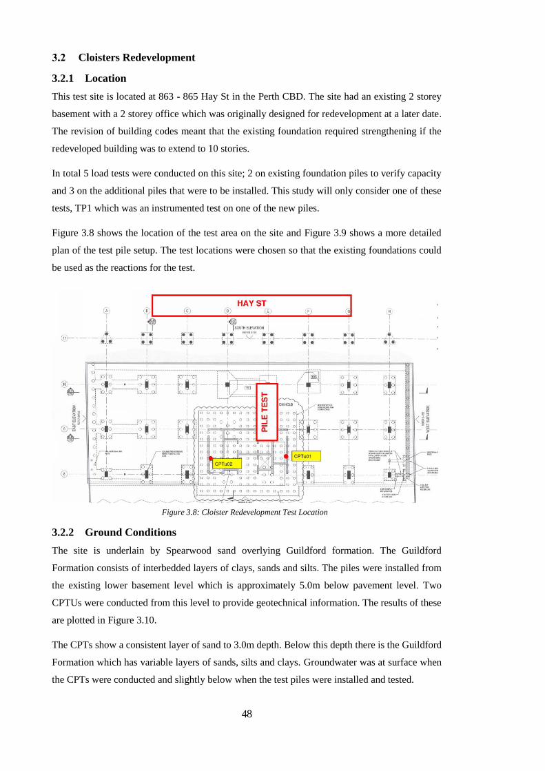
48
Cloisters Redevelopment
3.2.1 Location
This test site is located at 863 - 865 Hay St in the Perth CBD. The site had an existing 2 storey
basement with a 2 storey office which was originally designed for redevelopment at a later date.
The revision of building codes meant that the existing foundation required strengthening if the
redeveloped building was to extend to 10 stories.
In total 5 load tests were conducted on this site; 2 on existing foundation piles to verify capacity
and 3 on the additional piles that were to be installed. This study will only consider one of these
tests, TP1 which was an instrumented test on one of the new piles.
Figure 3.8 shows the location of the test area on the site and Figure 3.9 shows a more detailed
plan of the test pile setup. The test locations were chosen so that the existing foundations could
be used as the reactions for the test.
3.2.2 Ground Conditions
The site is underlain by Spearwood sand overlying Guildford formation. The Guildford
Formation consists of interbedded layers of clays, sands and silts. The piles were installed from
the existing lower basement level which is approximately 5.0m below pavement level. Two
CPTUs were conducted from this level to provide geotechnical information. The results of these
are plotted in Figure 3.10.
The CPTs show a consistent layer of sand to 3.0m depth. Below this depth there is the Guildford
Formation which has variable layers of sands, silts and clays. Groundwater was at surface when
the CPTs were conducted and slightly below when the test piles were installed and tested.
Figure 3.8: Cloister Redevelopment Test Location

49
Figure 3.9: Cloisters Redevelopment Test Layout
Figure 3.10: Cloisters Redevelopment CPT Profiles

50
3.2.3 Test Pile Details
The test pile on this site was a 300mm dia. 9.2m long CFA pile. Because of the headroom
restrictions (2.2m) this was installed using sectional augers. Table 3.2 summarises the pile
details. The pile was instrumented with two pairs of electrical resistance strain gauge sister bars
manufactured by CMR Technologies and were placed at levels of 1.5m and 9.0m.
Reaction for this test was provided by a series of loading beams and tension bars were anchored
in existing pile caps.
Table 3.2: Cloisters Redevelopment Test Pile Details
Pile Dimensions
Dia. 300mm
Depth 9.2m
Install RL 9.75m RL
Installation
Installation Method Sectional CFA
Rig Belpile PIG Rig
Installation Date 21/12/2012
Concrete
f'c 40 MPa (Neat cement grout)
Max Aggregate Nil
Cement Type GP
Slump N/A
Reinforcement
Main Bar 6N20 top of pile, 6N16 bottom of pile
Cage OD 190mm
Ligatures N10@200mm
Length 9.0m
Instrumentation
Type CMR Technologies Sister Bars (Electrical Resistance)
Strain Gauge Levels 1.5m and 9.0m

51
3.2.4 Testing Procedure and Results
The pile was loaded using the standard static load test procedure. The pile was loaded to its
working load, maintained at this load to check for creep, unloaded, and finally loaded to failure;
see Figure 3.11.
Figure 3.12 shows the test pile set-up. The pile was loaded using a 100t jack. Load was measured
by a standard load cell and displacement was measured at four points on the pile head using
displacement transducers attached to reference beams. The hydraulic cylinder was controlled by a
specially made computer program that also logs all the data.
Figure 3.11: Cloisters Redevelopment Test Loading Rate
Figure 3.12: Cloisters Redevelopment Load Test Setup
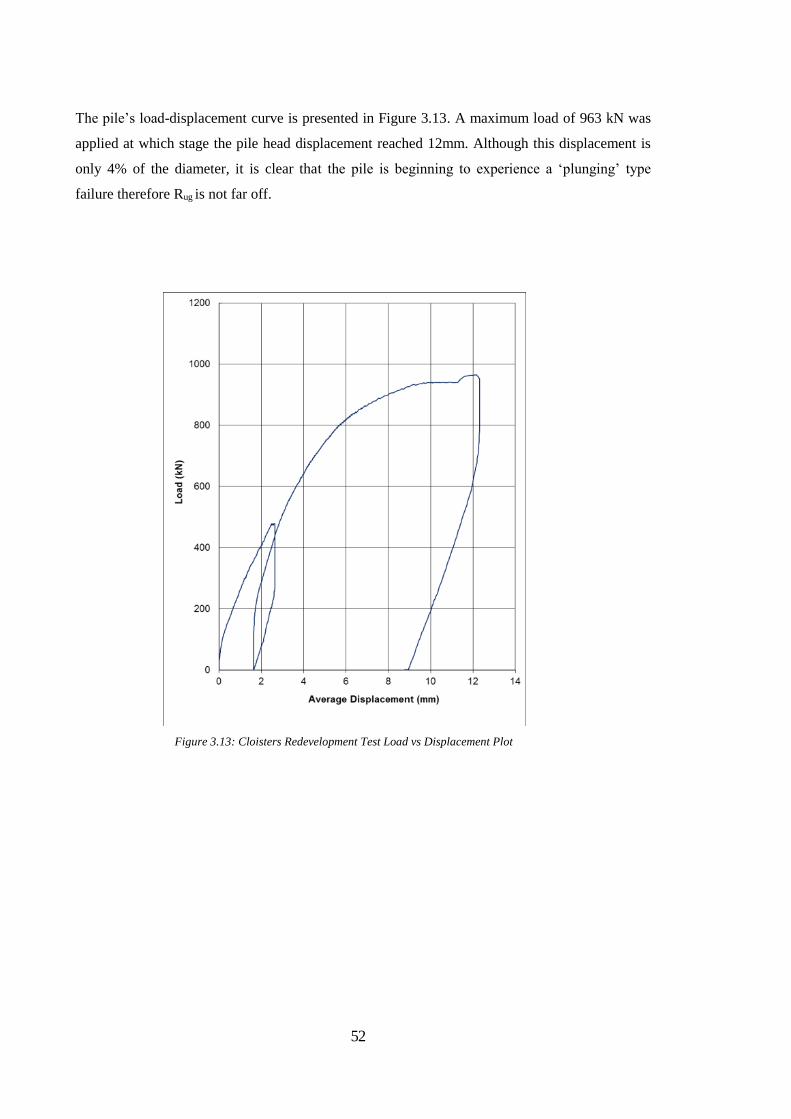
52
The pile’s load-displacement curve is presented in Figure 3.13. A maximum load of 963 kN was
applied at which stage the pile head displacement reached 12mm. Although this displacement is
only 4% of the diameter, it is clear that the pile is beginning to experience a ‘plunging’ type
failure therefore Rug is not far off.
Figure 3.13: Cloisters Redevelopment Test Load vs Displacement Plot

53
Cockburn Gateway Shopping Centre
3.3.1 Location
This test site is located at the Cockburn Gateway Shopping Centre which occupies a large site
South West of the Intersection between Kwinana Freeway and Beeliar Drive. The project was
an expansion to the existing shopping centre on vacant land. The expansion involved the top
down construction of a single storey basement carpark, one floor of retail and a rooftop carpark.
Figure 3.14 shows the new development highlighted and the test location identified.
There were two tests conducted on this site and both were instrumented. Figure 3.15 shows a
detailed layout of the test location.
TEST
Figure 3.15: Cockburn Gateway Test Pile Location
Figure 3.14: Cockburn Gateway Test Pile Layout

54
3.3.2 Ground Conditions
The site is underlain by Bassendean sand becoming very dense at depth. The overall site was
vast and a large number of CPTs were conducted across site to provide geotechnical
information. There were three CPTs conducted as part of the test program CPT 20, CPT 21 and
CPT 22A whose locations are shown in Figure 3.14. The CPTs are plotted in Figure 3.16.
Groundwater was approximately 9.0m below the toe of the piles
3.3.3 Test Pile Details
Two piles were tested on this site TP1 and TP2.
TP1 was a CFA pile 500mm diameter 9.2m long and TP2 was a 500/950 ‘belpile’ 9.2m long. A
belpile is a enlarged base pile drilled under bentonite where the top of the enlargement has the
same diameter as the bottom. In this case, the enlargement had a height of 950mm. Table 3.3
summarises the test pile details. TP2, the 500/950 ‘belpile’ was instrumented with pairs of
electrical resistance strain gauges which were manufactured by CMR Technologies. These were
placed at 1.5m, 3.5m and 7.5m. The top strain gauges were to facilitate analysis, the gauges at
Figure 3.16: Cockburn Gateway Test Pile CPTs
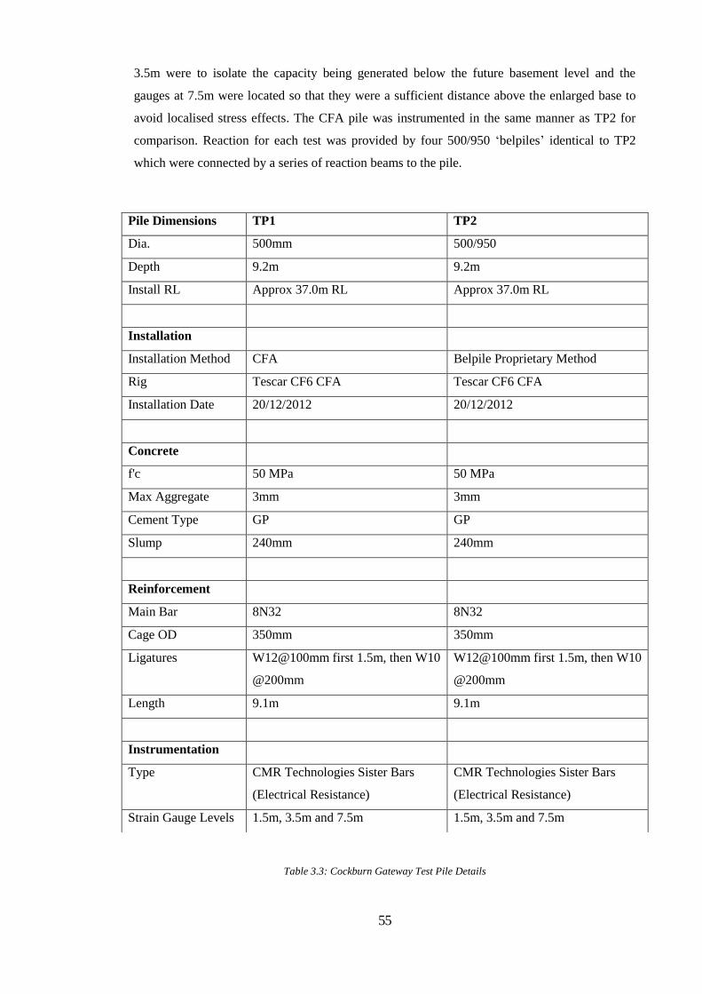
55
3.5m were to isolate the capacity being generated below the future basement level and the
gauges at 7.5m were located so that they were a sufficient distance above the enlarged base to
avoid localised stress effects. The CFA pile was instrumented in the same manner as TP2 for
comparison. Reaction for each test was provided by four 500/950 ‘belpiles’ identical to TP2
which were connected by a series of reaction beams to the pile.
Table 3.3: Cockburn Gateway Test Pile Details
Pile Dimensions TP1 TP2
Dia. 500mm 500/950
Depth 9.2m 9.2m
Install RL Approx 37.0m RL Approx 37.0m RL
Installation
Installation Method CFA Belpile Proprietary Method
Rig Tescar CF6 CFA Tescar CF6 CFA
Installation Date 20/12/2012 20/12/2012
Concrete
f'c 50 MPa 50 MPa
Max Aggregate 3mm 3mm
Cement Type GP GP
Slump 240mm 240mm
Reinforcement
Main Bar 8N32 8N32
Cage OD 350mm 350mm
Ligatures W12@100mm first 1.5m, then W10
@200mm
W12@100mm first 1.5m, then W10
@200mm
Length 9.1m 9.1m
Instrumentation
Type CMR Technologies Sister Bars
(Electrical Resistance)
CMR Technologies Sister Bars
(Electrical Resistance)
Strain Gauge Levels 1.5m, 3.5m and 7.5m 1.5m, 3.5m and 7.5m

56
3.3.4 Testing Procedure and Results
As can be seen in Figure 3.17 the piles were loaded using 6 x 100t jacks. Load was measured by
a load cell and displacement was measured at four points at the pile head using displacement
transducers attached to reference beams. The hydraulic cylinders were controlled by a specially
coded computer program that also logs all of the data.
The piles were loaded using a standard static load test procedure. The pile was loaded to its
working load, maintained at this load to check for creep, unloaded, and finally loaded to failure;
see Figure 3.18.
TP1 was initially loaded to 600kN when two things were noticed; one of the displacement
sensors was placed in a position where it was interacting with the test setup and the gauges
CCA3.5 and CCA7.5 were reading the same strain. Gauges CCB3.5 and CCB7.5 were similarly
reading the same strain. (To illustrate how similar they were the linest function in Excel gives a
correlation between both sets of data with a slope of 0.998 and an R2 value of 0.99999)
The author has never experienced that level of correlation even when the strain gauges are at the
same level. For two pairs of strain gauges to do this in one test when they are at different levels
is not considered possible. It was deemed to be more than just a mix up between CCA3.5 and
CCA7.5 or vice versa as it is still considered impossible for the reading to be so close. It was
determined there was some issue with how these strain gauges had been wired to the logging
system. TP1 was therefore unloaded to rectify the problems and the pile test was restarted as per
Figure 3.18 (a).
Figure 3.17: Cockburn Gateway Pile Test Setup

57
TP2 did not experience the same problems as TP1 and its loading history is shown in Figure
3.18 (b).
TP1 Results
The pile’s load-displacement curve measured after the re-start described above is presented in
Figure 3.19. It should be noted that all readings (displacement, load and strain) were reset to
zero for the test. This, as expected, resulted in a stiff response up to the maximum previously
applied load of 600kN; this response is not considered to have a large effect on the remainder of
the test, which involved application of a final load of 4,473 kN at a displacement of 53mm. The
load at a displacement of 0.1D was 4,444 kN which is considered to be RUG. The pile response
was as expected and is evidently capable of developing more load well past 0.1D (as is typical
for bored piles in sand).
Figure 3.18: Cockburn Gateway Test Loading Rates (left) TP1, (right) TP2
Figure 3.19: Cockburn Gateway TP1 Load Displacement Curve

58
TP2 Results
The pile’s load-displacement curve for pile TP2 at Cockburn is plotted in Figure 3.20. This
pile’s ultimate capacity exceeded the capacity of the loading system. A maximum load of 5,775
kN was applied at which point the pile head had displaced by 50mm. On inspection of Figure
3.20, it may be inferred that the ultimate capacity at a displacement of 10% of the pile base
(=95mm) is in the order of 6.5 – 7.0 MN
Figure 3.20: Cockburn Gateway TP2 Load Displacement Curve
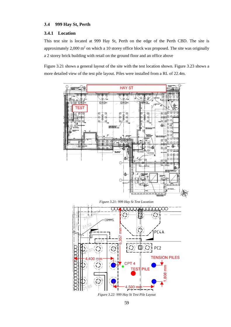
59
999 Hay St, Perth
3.4.1 Location
This test site is located at 999 Hay St, Perth on the edge of the Perth CBD. The site is
approximately 2,000 m2 on which a 10 storey office block was proposed. The site was originally
a 2 storey brick building with retail on the ground floor and an office above
Figure 3.21 shows a general layout of the site with the test location shown. Figure 3.23 shows a
more detailed view of the test pile layout. Piles were installed from a RL of 22.4m.
Figure 3.21: 999 Hay St Test Location
Figure 3.22: 999 Hay St Test Pile Layout

60
3.4.2 Ground Conditions
The site is underlain by sand derived from Tamala Limestone getting very dense at depth. Five
CPTs were conducted on site and produced consistent results. CPT 4 was very close to the load
test so is the only CPT plotted in Figure 3.23; it is noted that this CPT was conducted before any
piles were installed on site so isn’t affected by any drilling operations. Groundwater was at 10m
below surface so was just below the pile toe
Figure 3.23: 999 Hay St Test Pile CPT
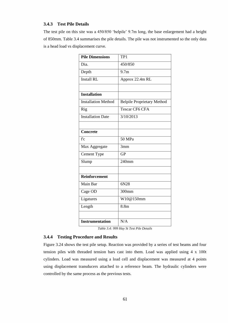
61
3.4.3 Test Pile Details
The test pile on this site was a 450/850 ‘belpile’ 9.7m long, the base enlargement had a height
of 850mm. Table 3.4 summarises the pile details. The pile was not instrumented so the only data
is a head load vs displacement curve.
Pile Dimensions TP1
Dia. 450/850
Depth 9.7m
Install RL Approx 22.4m RL
Installation
Installation Method Belpile Proprietary Method
Rig Tescar CF6 CFA
Installation Date 3/10/2013
Concrete
f'c 50 MPa
Max Aggregate 3mm
Cement Type GP
Slump 240mm
Reinforcement
Main Bar 6N28
Cage OD 300mm
Ligatures W10@150mm
Length 8.8m
Instrumentation N/A
Table 3.4: 999 Hay St Test Pile Details
3.4.4 Testing Procedure and Results
Figure 3.24 shows the test pile setup. Reaction was provided by a series of test beams and four
tension piles with threaded tension bars cast into them. Load was applied using 4 x 100t
cylinders. Load was measured using a load cell and displacement was measured at 4 points
using displacement transducers attached to a reference beam. The hydraulic cylinders were
controlled by the same process as the previous tests.

62
The pile was loaded in a typical fashion with a working load of 1,500 kN being applied and held
before being unloaded and reloaded to failure (Figure 3.25).
The measured load displacement curve can be seen in Figure 3.26, where it is shown that the
pile reached an ultimate geotechnical load (RUG) of 3,290 kN at 85mm of displacement. The pile
is still gaining load at this point so a plunging type failure has not occurred.
Figure 3.24: 999 Hay St Pile Test Setup
Figure 3.25: 999 Hay St Pile Loading Rate

63
Figure 3.26: 999 Hay St Load vs Displacement Curve

64
UWA IOMRC
3.5.1 Location
This site is located on the University of Western Australia’s Crawley campus, on Fairway Drive
at Entrance 4. The site is approximately 4,000 m2 and was previously an asphalt carpark. The
new building is to be a 6 storey marine research facility housing a number of centrifuges.
Figure 3.27 shows the site layout with the location of the two test piles marked. Figure 3.28 and
3.29 show the detailed view of each respective test.
Figure 3.27: UWA Test Locations
Figure 3.28: UWA Test Pile 1 Layout

65
3.5.2 Ground Conditions
The site is underlain by sand derived from Tamala Limestone getting very dense at depth. CPT
results were consistent across site. CPT 2 was conducted in the original geotechnical report and
is in close proximity to TP1 and CPT TP2 was conducted after the pile was installed so was
conducted 5.0m away from the test. The CPT results are displayed in Figure 3.30. The ground
water is relatively shallow approximately 4.0m below ground level.
Figure 3.29: UWA Test Pile 2 Layout
Figure 3.30: UWA Test CPTs

66
3.5.3 Test Pile Details
The test piles were both 600mm dia., 14m long CFA piles. Table 3.5 summarises the pile
details. The pile was not instrumented so the only the head load vs displacement curve was
recorded.
Pile Dimensions TP1 TP1
Dia. 600mm 600mm
Depth 14.0 14.0
Install RL Approx 5.3m RL Approx 5.3m RL
Installation
Installation
Method
CFA CFA
Rig MAIT HR130 CFA MAIT HR130 CFA
Installation Date 3/5 16/5
Concrete
f'c 50 MPa 50 MPa
Max Aggregate 3mm 3mm
Cement Type GP GP
Slump 240mm 240mm
Reinforcement
Main Bar 8N24 8N24
Cage OD 450mm 450mm
Ligatures W10@200mm W10@200mm
Length 12.0m 12.0m
Instrumentation N/A N/A
Table 3.5: UWA Test Pile Details
3.5.4 Testing Procedure and Results
Figure 3.31 shows the test pile setup. Reaction was provided by a series of test beams and four
tension piles with threaded tension bars cast into them. Load was applied using 4 x 100t
cylinders. Load was measured using a load cell and displacement was measured at 4 points
using displacement transducers attached to a reference beam. The hydraulic cylinders were
controlled by the same process as the previous tests.
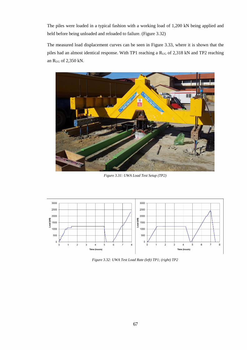
67
The piles were loaded in a typical fashion with a working load of 1,200 kN being applied and
held before being unloaded and reloaded to failure. (Figure 3.32)
The measured load displacement curves can be seen in Figure 3.33, where it is shown that the
piles had an almost identical response. With TP1 reaching a RUG of 2,318 kN and TP2 reaching
an RUG of 2,350 kN.
Figure 3.32: UWA Test Load Rate (left) TP1; (right) TP2
Figure 3.31: UWA Load Test Setup (TP2)
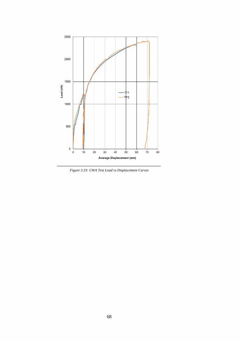
68
Figure 3.33: UWA Test Load vs Displacement Curves
69
Chapter 4
Measuring Load Distribution in Bored Piles

70
4 Measuring Load Distribution in Bored Piles
This chapter examines the load distributions measured in the instrumented test piles using the
following techniques outlined in Chapter 2:
- Uncorrected Area Method
- Transformed Area Method
- Implicit Method
- Secant Method
- Tangent Method
4.1.1 500 Hay St Strain Gauge Analysis
Figure 4.1 shows a plot of strain vs time for all the strain gauges. Taking a broad look at the
overall strain gauge data it can be seen that:
-All 10 strain gauges survived the test
-All pairs of strain gauges were reacting together
-Strain reduced with distance from the pile head
-The top two strain gauges had the largest difference which is likely to be a result of
slight eccentricity of the head load
-The bottom pair of gauges also had some deviation suggesting that there were small
bending stresses at the pile base
Figure 4.1: 500 Hay St Strain vs time
71
The gauges therefore appear to be behaving correctly and that good quality data was obtained.
As mentioned previously, the bottom strain gauge level is 1.9m above the pile toe. Therefore,
the shaft friction calculated between depths of 10.0m and 13.5m is also assumed to be the shaft
friction between 13.5m and the pile base at 15.4m.
4.1.2 Uncorrected Area Method
No specific ‘Modulus of Elasticity’ test was conducted so, to apply this method, a modulus has
to be derived indirectly from cylinder strengths. The cylinders were crushed at 7 days whilst the
test was conducted at 11 days and therefore the cylinder strength at 11 days was estimated using
the logarithmic relationship described by Neville (2014).
7 Day Strength 44 MPa
28 Day Strength 68 MPa
Estimated 11-day Strength 51 MPa
Table 4.1: 500 Hay St Concrete Strengths
Using the 11-day strength of 51 MPa in Equation 2.5, an estimated modulus of elasticity of 34.4
GPa is obtained for use in the Uncorrected Method. Applying this to the data obtained in the test
the following results are obtained at a pile head displacement of 60mm (=D/10):
Load at Pile Head 5212 kN Compared to 4664 kN measured
Load at Pile Base 1586 kN
Pressure at Pile
Base
5626 kPa
Table 4.2: 500 Hay St Uncorrected Area Strain Gauge Interpretation
It can readily be seen that, using this method, the head load is overestimated by 600kN which is
an error that is likely to be carried on down the pile; it follows that there is potentially a 40%
error in the base resistance. The Shaft friction vs pile head displacement curves between each
gauge level using this method are plotted on Figure 4.2.
What is immediately obvious on Figure 4.2 is that the interpreted shaft friction is, is some cases,
still increasing even after a pile head displacement of 60mm; this result is contrary to commonly
observed shaft friction t-z curves. The distribution of shaft friction is also contrary to commonly
held design assumptions with the highest calculated friction at the top of the pile where the CPT
tip resistances are lowest. The shaft friction between 6.0m and 10.0m is also a bit surprising as
the soil profile is not significantly worse at this depth. The average shaft friction over the strain
gauges is 130 kPa which is high but not unrealistic for this sand.

72
It can be concluded that, as may be expected, the ‘Uncorrected Area Method’ has some
shortcomings.
4.1.3 Transformed Area Method
The test pile was reinforced with 8N28 bars which gives a steel area of 4,928 mm2. Using
Equation 2.6 and the modulus used by the Uncorrected Area Method an equivalent axial
Young’s Modulus of 37.29 GPa is calculated.
As this method is very similar to the Uncorrected Area Method (except that it employs a higher
modulus) similar results were obtained. The primary differences were that the Transformed
Area method gives a higher head load, shaft friction values about 10% higher and a higher base
load. As the plot for shaft friction is almost identical to the uncorrected area method it has not
been included here.
Load at Pile Head 5650 kN Compared to 4664 kN measured
Load at pile Base 1708 kN
Pressure at Pile
Base
6059 kPa
Table 4.3: 500 Hay St Transformed Area Strain Gauge Interpretation
Although it was expected that this method should produce a more accurate calculation of the
pile loads the opposite is true. The already high modulus value calculated for the concrete has
been increased further by including the steel which has led to an even higher estimate of pile
head load of 5,650 kN compared to the measured value of 4,664 kN.
0
20
40
60
80
100
120
140
160
180
200
0 10 20 30 40 50 60
Pile
Sh
aft
Fric
tio
n (
kPa)
Pile Head Displacment (mm)
0.5m to 3.0m
3.0m to 6.0m
6.0m to 10.0m
10.0m to 13.5m
0.5m to 13.5m
Figure 4.2: 500 Hay St Shaft friction vs head displacement determined using the un-corrected
area method

73
4.1.4 Implicit Method
This method required no special modifications or inputs to the data. It is the first of the methods
examined to take into account the non-linearity of the pile’s modulus and calibrate the test to the
top strain gauge. This method by definition gets the pile head load correct which immediately
gives more confidence in the accuracy of this method. Table 4.4 shows the interpreted loads
using this approach.
Load at Pile Head 4664 kN Compared to 4664 kN Measured
Load at Pile Base 1410 kN
Pressure at Pile Base 5002 kPa
Table 4.4: 500 Hay St Implicit Method Strain Gauge Interpretation
This method gave a comparable distribution of shaft friction to that obtained with the methods
examined above. Shaft friction has reduced from the uncorrected area method (as the pile head
load is lower). The highest shaft friction is still being developed near the pile head and it is still
increasing right up to pile failure.
This method performs better than the previous two as it gets the head load right. However, in
terms of the pile load distribution apart from a small correction in the magnitude of the friction,
this method still suffers from the same assumptions as the other methods.
Figure 4.3: 500 Hay St Shaft friction vs head displacement determined using the implicit method
0
20
40
60
80
100
120
140
160
180
0 10 20 30 40 50 60
Pile
Sh
aft
Fric
tio
n (
kPa)
Pile Head Displacement (mm)
0.5m to 3.0m
3.0m to 6.0m
6.0m to 10.0m
10.0m to 13.5m
0.5m to 13.5m

74
4.1.5 Secant Modulus Method
This method calculated the modulus from the following relationship which was derived from
the pile head load and upper set of strain gauges:
𝐸 = −0.0071 . 휀 + 34.473
This equation is plotted in Figure 4.4 and was derived using a polynomial trend line in
Microsoft Excel (with R2 value of 0.9999). Using this relationship, the following interpreted
loads were calculated:
Load at Pile Head 4639 kN Compared to 4664 kN Measured
Load at Pile Base 1598 kN
Pressure at Pile Base 5667 kPa
Table 4.5: 500 Hay St Secant Method Strain Gauge Interpretation
This method has a very small error in the head load but again suffers the same problems as the
previous methods; with shaft friction increasing well into pile failure and an
abnormal/unexpected distribution of shaft shear stress.
Figure 4.4: 500 Hay St Secant Modulus Top Strain Gauge trendline
Equation 4.1

75
4.1.6 Tangent Modulus Method
Figure 4.5a plots the strain at each level against the pile head load. This plot allows a quick
assessment of the applicability of the Tangent Modulus Method. As can be seen the plot
towards the end of the test all of the strain gauge readings have a similar slope. This indicates
that peak shaft friction has been exceeded at all levels and there should be sufficient data to
derive specific modulus values for each level.
Figure 4.5: 500 Hay St Shaft friction vs head displacement determined using the secant method
Figure 4.5a: 500 Hay St Strain vs Head Load

76
Application of this method required some modification to the data. With the type of setup used
in this test over 1000 data points have been recorded. Although this produces more detailed
plots it creates a lot of noise once it is differentiated. Figure 4.6 plots the calculated tangent
moduli of the gauges at 0.5m using all available data points.
A general trend can be recognised in Figure 4.6 however the noise present in this data set makes
it difficult to accurately define a Tangent Modulus line. The trendline generated by Microsoft
Excel is displayed on the plot however it has been greatly distorted by the noise and not
representative of the trend. A more logical line can be drawn manually however this still won’t
be reliable enough to complete the analysis. In order to analyse the data reliably it is evident that
a smaller set of data is needed so that the Δstress/Δstrain is calculated over a larger range which
will average the data.
Figure 4.7 is the same data but has been reduced to load steps of 50kN. The data points between
these load steps have effectively been ‘deleted’. This has made the data much easier to interpret,
although a number of ‘dips’ in the plot are now evident. These coincide with the hold periods
during the pile loading and are a result of concrete creep. These dips distort the trendline but
cannot be ignored as the concrete is creeping throughout the test and to ignore these points
would distort the rest of the data.
It was found that reducing the data set to 21 points (250kN steps) provided a set that could be
analysed relatively easily. Figure 4.8 shows a plot of Δstress/Δstrain at each strain level reduced
to steps of 250 kN.
Figure 4.6: 500 Hay St Tangent Modulus Raw Data Noise
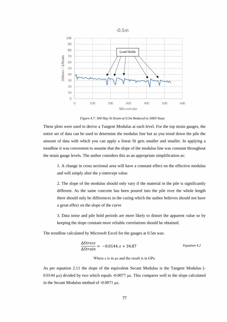
77
These plots were used to derive a Tangent Modulus at each level. For the top strain gauges, the
entire set of data can be used to determine the modulus line but as you trend down the pile the
amount of data with which you can apply a linear fit gets smaller and smaller. In applying a
trendline it was convenient to assume that the slope of the modulus line was constant throughout
the strain gauge levels. The author considers this as an appropriate simplification as:
1. A change in cross sectional area will have a constant effect on the effective modulus
and will simply alter the y-intercept value.
2. The slope of the modulus should only vary if the material in the pile is significantly
different. As the same concrete has been poured into the pile over the whole length
there should only be differences in the curing which the author believes should not have
a great effect on the slope of the curve
3. Data noise and pile hold periods are more likely to distort the apparent value so by
keeping the slope constant more reliable correlations should be obtained.
The trendline calculated by Microsoft Excel for the gauges at 0.5m was:
∆𝑆𝑡𝑟𝑒𝑠𝑠
∆𝑆𝑡𝑟𝑎𝑖𝑛= −0.0144. 휀 + 34.87
Where ε is in µε and the result is in GPa
As per equation 2.11 the slope of the equivalent Secant Modulus is the Tangent Modulus (-
0.0144 µε) divided by two which equals -0.0077 µε. This compares well to the slope calculated
in the Secant Modulus method of -0.0071 µε.
Equation 4.2
Figure 4.7: 500 Hay St Strain at 0.5m Reduced to 50kN Steps
Load Holds

78
The -0.0144 has been used as the assumed gradient of the line of best fit for the rest of the
gauges. These lines can be seen in Figure 4.8. The lines have been fitted once the ΔStress /
ΔStrain levels off which indicates that the pile has ceased generating capacity above this point.
Table 4.6 shows a summary of the y-intercept values. There is more variation in the y-intercept
concrete modulus values than the author would expect. Possible reasons for this variation
include; changes in diameter of the pile, variations in the curing conditions in the ground (i.e
groundwater depth and permeability) and the increasing pressure in the wet concrete column
increasing the density of the concrete at depth.
All strain gauge levels get a good fit using the slope derived from the gauge at 0.5m and only
altering the y-intercept. Although not displayed above the gauge at 13.5m didn’t level off at the
20mm head displacement as expected but continued to a head displacement of 30mm before
levelling off (approximately 125µε in Figure 4.8). This is credible as the pile axial compression
at this point will be around 5mm so the relative shaft movement is 25mm which is within
observed dilation displacement range.
Figure 4.8: 500 Hay St Tangent Method Line of best fits for the 5 strain gauge levels

79
Gauge y-intercept Strain at 20mm head displacement
0.5m 34.87 339
3.0m 39.5 286
6.0m 43.5 224
10.0m 41 163
13.5m 43 84
Table 4.6: 500 Hay St Tangent Method Modulus Summary
Using the above correlations, we get the following interpretation of the load test:
Load at Pile Head 4697 kN Compared to 4664 kN Measured
Load at Pile Base 2028 kN
Pressure at Pile Base 7195 kPa
Table 4.7: 500 Hay St Tangent Method Strain Gauge Interpretation
This method creates a different interpretation of the load test compared to the other methods.
This method has seen a decrease of the average shaft friction to 90 kPa, the shaft frictions have
levelled off after peaking and there is a tendency for increasing shaft friction with depth which
is in line with the increasing CPT resistance with depth on this site
Figure 4.9 shows that the shaft friction between 10.0m and 13.5m has taken approximately
24mm of head displacement to peak. This is less than what it took for the ΔStress / ΔStrain plot
to level off which is likely a result of reducing the data to large load steps.
Compared to the other methods the plots in Figure 4.9 are closer to the shear stress data
produced using direct shear stress transducers in Figure 2.7. This increases confidence in this
interpretation.

80
4.1.7 Comparison
To aid comparison with the tests analysed by Lam and Jefferis (2011), Figure 4.10 compares the
ultimate shaft and base values that each method calculated. The range of shaft frictions and base
resistances is wide which could have serious implications if incorrect values were then applied
to piles of different sizes or at different project locations.
The Tangent Method appears to give the most credible interpretation to this test as:
- The calculated shaft frictions reach a maximum ultimate values
- The shaft friction increases with increasing CPT tip resistance
- Large shaft frictions are not interpreted near the pile head
It is clear that the Tangent Method calculates a distinct interpretation to the other methods as it
is calibrating each strain gauge. The other methods all suffer from the same assumption that
each section of the pile is identical. This assumption holds true for other pile types like driven
steel tubes or driven precast piles. However, in the case of bored piles and especially CFA piles,
this test has shown that the assumption of a constant EA value is not valid.
Figure 4.9: 500 Hay St Shaft friction vs head displacement determined using the tangent method
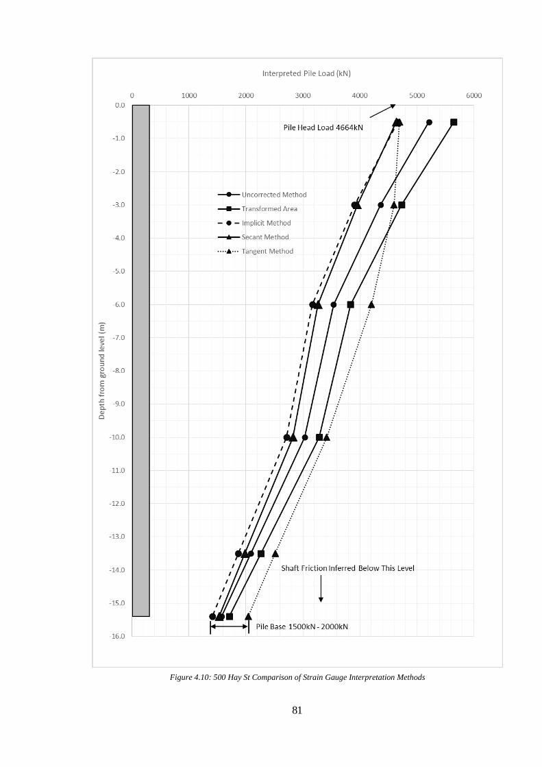
81
Figure 4.10: 500 Hay St Comparison of Strain Gauge Interpretation Methods

82
Cloisters Redevelopment Strain Gauge Analysis
Figure 4.11 plots strain vs time for the Cloisters Redevelopment Test. All 4 strain gauges
survived the test and taking a basic look at the data it can be seen that:
- All pairs of strain gauges were reacting together
- There was a decreasing amount of strain down the pile
-The top two strain gauges had a difference of 270µε which indicates bending at the
top of the pile caused by load eccentricity
- The bottom pair were very similar indicating that they worked reliably
- The large difference between the strain at 1.5m and 9.0m indicates most of the pile’s
capacity is provided by shaft friction
These observations indicate that the gauges appear to be behaving correctly and that good
quality has been obtained.
4.2.1 Uncorrected Area Method
No specific Modulus of Elasticity test was conducted for this pile and therefore a modulus was
derived from Figure 2.4. This project used a grout with a w/c ratio of 0.5 which gives an
estimated modulus of elasticity of 10 GPa. Applying this to the data obtained in the test gives
the results presented in Table 4.8.
Figure 4.11: Cloisters Redevelopment Test Strain vs time
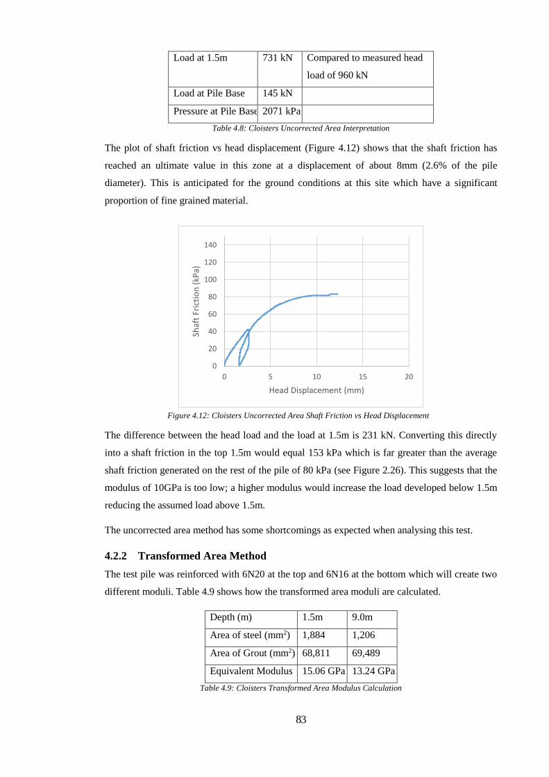
83
Load at 1.5m 731 kN Compared to measured head
load of 960 kN
Load at Pile Base 145 kN
Pressure at Pile Base 2071 kPa
Table 4.8: Cloisters Uncorrected Area Interpretation
The plot of shaft friction vs head displacement (Figure 4.12) shows that the shaft friction has
reached an ultimate value in this zone at a displacement of about 8mm (2.6% of the pile
diameter). This is anticipated for the ground conditions at this site which have a significant
proportion of fine grained material.
The difference between the head load and the load at 1.5m is 231 kN. Converting this directly
into a shaft friction in the top 1.5m would equal 153 kPa which is far greater than the average
shaft friction generated on the rest of the pile of 80 kPa (see Figure 2.26). This suggests that the
modulus of 10GPa is too low; a higher modulus would increase the load developed below 1.5m
reducing the assumed load above 1.5m.
The uncorrected area method has some shortcomings as expected when analysing this test.
4.2.2 Transformed Area Method
The test pile was reinforced with 6N20 at the top and 6N16 at the bottom which will create two
different moduli. Table 4.9 shows how the transformed area moduli are calculated.
Depth (m) 1.5m 9.0m
Area of steel (mm2) 1,884 1,206
Area of Grout (mm2) 68,811 69,489
Equivalent Modulus 15.06 GPa 13.24 GPa
Table 4.9: Cloisters Transformed Area Modulus Calculation
0
20
40
60
80
100
120
140
0 5 10 15 20
Shaf
t Fr
icti
on
(kP
a)
Head Displacement (mm)
Figure 4.12: Cloisters Uncorrected Area Shaft Friction vs Head Displacement

84
This method produced modulus values that are 30% to 50% higher than the modulus of the
grout alone. As there is a large percentage of steel (up to 2.7%) and the modulus of grout is low
the inclusion of steel in the calculation has had a large effect. Table 4.10 shows the loads
determined using this method.
Load at Pile Head 967 kN Compared to measured head load of 960 kN
Load at Pile Base 217 kN
Pressure at Pile Base 3,100 kPa
Table 4.10: Cloisters Transformed Area Interpretation
The higher moduli have increased the calculated load on the shaft between 1.5m and 9.0m,
giving an average shaft friction of 105kPa; this is 25% higher than that given by the uncorrected
area method. This method has practically eliminated all shaft friction in the top 1.5m which is
not realistic and is indicating that the modulus calculated is a bit high.
4.2.3 Implicit Method
To utilise this method, it had to be assumed that the strain at 1.5m is equivalent to the strain at
the pile head. This will have the effect of ignoring the top 1.5m of the pile and will slightly
increase the calculated average shaft friction as it assumes that the shaft friction is developed
over a shorter length than normal. This method produced the following results:
Load at Pile Head 960 kN Compared to measured head load of 960 kN
Load at Pile Base 189 kN
Pressure at Pile Base 2,700 kPa
Table 4.11: Cloisters Implicit Method Interpretation
As expected, this method predicts the pile head load exactly and has predicted a slightly higher
shaft friction than the Transformed Area method. This higher shaft friction has resulted in a
drop in the base capacity.
4.2.4 Secant Modulus Method
As with the Implicit Method it is necessary to make the assumption that the gauge at 1.5m is
equivalent to the strain at the pile head. It is expected that this assumption will create small
errors at low strains.
This method calculated that the modulus followed the following relationship:
𝐸 = −0.0012 . 휀 + 14.339
This equation is plotted in Figure 4.13 and was calculated using a polynomial trend line in
Microsoft Excel. This trend line had an R2 value of 0.9952.
Equation 4.3

85
It can be seen that the initial pile data deviates from the calculated line; this is likely because a
small amount of shaft friction is developing above the strain gauge level.
Applying this relationship to all of the gauges gives the following interpretation:
Load at -1.5m 956 kN Compared to measured head load of 960 kN
Load at Pile Base 203 kN
Pressure at Pile Base 2900 kPa
Table 4.12: Cloisters Secant Method Interpretation
Similarly to the Implicit Method, this interpretation suffers the same problem of the calculated
average shaft friction (of 106 kPa) may be a little high due to neglect of any friction generated
above the top level of strain gauges.
Figure 4.13: Cloisters Secant Modulus Top Strain Trendline
Figure 4.14: Cloisters Secant Method Shaft Friction vs Head Displacement
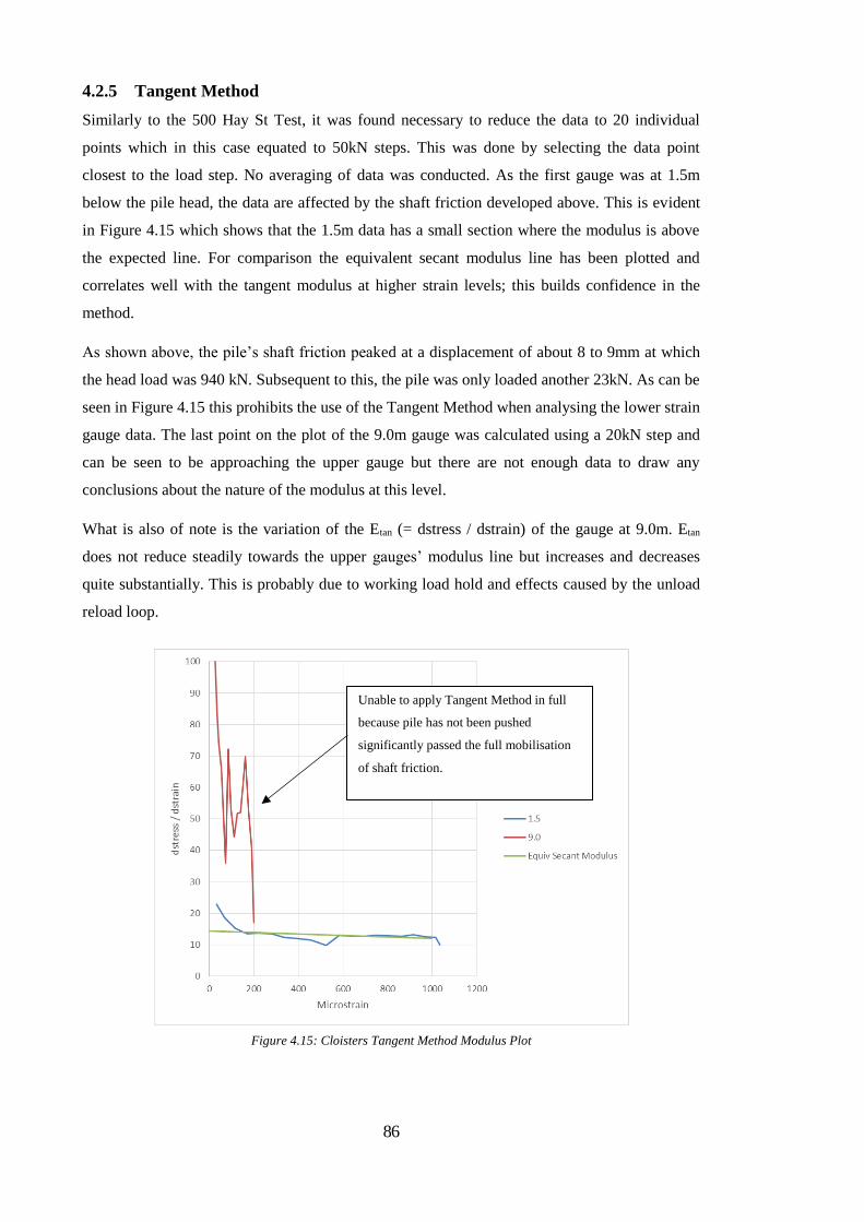
86
4.2.5 Tangent Method
Similarly to the 500 Hay St Test, it was found necessary to reduce the data to 20 individual
points which in this case equated to 50kN steps. This was done by selecting the data point
closest to the load step. No averaging of data was conducted. As the first gauge was at 1.5m
below the pile head, the data are affected by the shaft friction developed above. This is evident
in Figure 4.15 which shows that the 1.5m data has a small section where the modulus is above
the expected line. For comparison the equivalent secant modulus line has been plotted and
correlates well with the tangent modulus at higher strain levels; this builds confidence in the
method.
As shown above, the pile’s shaft friction peaked at a displacement of about 8 to 9mm at which
the head load was 940 kN. Subsequent to this, the pile was only loaded another 23kN. As can be
seen in Figure 4.15 this prohibits the use of the Tangent Method when analysing the lower strain
gauge data. The last point on the plot of the 9.0m gauge was calculated using a 20kN step and
can be seen to be approaching the upper gauge but there are not enough data to draw any
conclusions about the nature of the modulus at this level.
What is also of note is the variation of the Etan (= dstress / dstrain) of the gauge at 9.0m. Etan
does not reduce steadily towards the upper gauges’ modulus line but increases and decreases
quite substantially. This is probably due to working load hold and effects caused by the unload
reload loop.
Unable to apply Tangent Method in full
because pile has not been pushed
significantly passed the full mobilisation
of shaft friction.
Figure 4.15: Cloisters Tangent Method Modulus Plot

87
Figure 4.16 presents a plot of the variation of pile axial strain with pile head load. The gauge at
1.5m is approximately linear indicating that the pile shaft above is not generating much shaft
friction which allows most of the stress to reach the strain gauge. If a pile is displaced past its
peak shaft friction, then the lower gauge should have a gradient similar to that of the upper
gauge. This would indicate that between the gauges no further load is being transferred to the
soil. This test does not exhibit this response which prohibits the use of the Tangent Method to
back analyse the test.
It is clear that there are insufficient data from this test to apply the Tangent Method properly and
as such any analysis results would be identical to the Secant Method. This test also raises the
concern that the Tangent Method may not be effectively applied to piles with their bases
founded in clay as the base may not generate enough additional strain past the peak shaft
friction to derive the pile modulus.
4.2.6 Comparison
Figure 4.17 compares the results of the methods described above. The Tangent Method has been
left out for the reasons described above. In this case there has been good agreement between the
Transformed Area, Implicit and Secant Methods which increases the confidence in this
interpretation of the test.
These three interpretations predict essentially zero shaft friction in the top 1.5m. This could be a
result of the positioning of the top strain gauges or it could be that there is little resistance in this
Slope that would indicate shaft
friction has peaked and Tangent
Method Analysis is possible
Figure 4.16: Cloisters Pile Head Load vs Strain

88
zone. A small plastic sleeve was used to de-bond the pile from the slab and cast it above the slab
level. The actual depth of this sleeve is unknown but, if it continued 1.0m into the pile, it would
largely explain the low interpreted friction in the top 1.5m. The interpretation of the top strain
gauge by the Tangent Method also points to little resistance in this zone.
The main conclusion from this test is that application of the tangent method in tests on piles
with low base stiffness/capacity requires loads to be applied even after ultimate conditions are
attained. There may even be cases where the base capacity is so low that no that the Tangent
Method cannot be applied in its entirety.
This test has also shown that for slender piles (L/D = 30), a small change in the calculated shaft
friction causes a significant change in the pile base resistance. In this case a 4% change in shaft
friction has caused the calculated base resistance to decrease by 13%. It can be said that the
calculated base resistance in slender piles is, by nature, not as accurate as piles with a stronger
base response.
Figure 4.17: Cloisters Test Interpretation Comparison
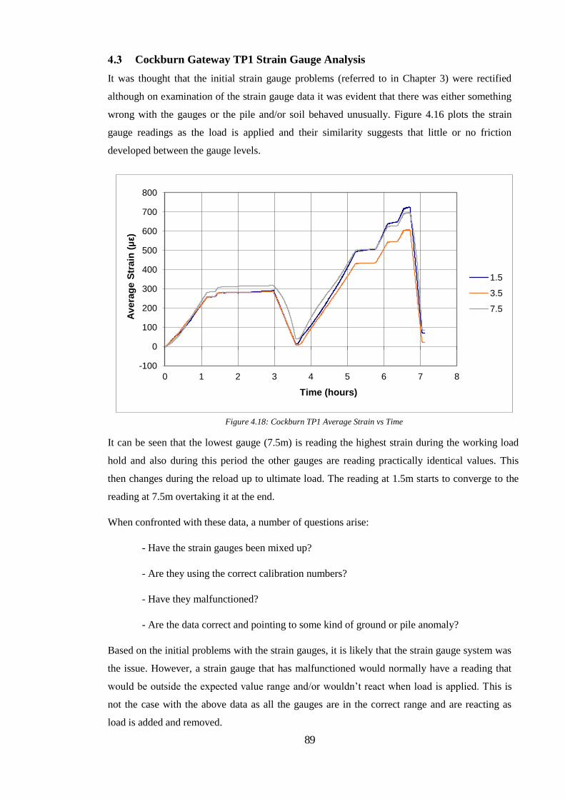
89
Cockburn Gateway TP1 Strain Gauge Analysis
It was thought that the initial strain gauge problems (referred to in Chapter 3) were rectified
although on examination of the strain gauge data it was evident that there was either something
wrong with the gauges or the pile and/or soil behaved unusually. Figure 4.16 plots the strain
gauge readings as the load is applied and their similarity suggests that little or no friction
developed between the gauge levels.
It can be seen that the lowest gauge (7.5m) is reading the highest strain during the working load
hold and also during this period the other gauges are reading practically identical values. This
then changes during the reload up to ultimate load. The reading at 1.5m starts to converge to the
reading at 7.5m overtaking it at the end.
When confronted with these data, a number of questions arise:
- Have the strain gauges been mixed up?
- Are they using the correct calibration numbers?
- Have they malfunctioned?
- Are the data correct and pointing to some kind of ground or pile anomaly?
Based on the initial problems with the strain gauges, it is likely that the strain gauge system was
the issue. However, a strain gauge that has malfunctioned would normally have a reading that
would be outside the expected value range and/or wouldn’t react when load is applied. This is
not the case with the above data as all the gauges are in the correct range and are reacting as
load is added and removed.
-100
0
100
200
300
400
500
600
700
800
0 1 2 3 4 5 6 7 8
Av
era
ge
Str
ain
(µε)
Time (hours)
1.5
3.5
7.5
Figure 4.18: Cockburn TP1 Average Strain vs Time

90
Normal strain gauge analysis of these data will lead to the conclusion that all the load is
developed below 7.5m and that there is a balance of positive and negative skin frictions above
this point. In these soils, the only mechanism potentially explaining this would be if the curing
process created extremely high (and unrealistic) residual loads such that positive ultimate skin
frictions acted over most of the shaft prior to the load test. In addition, taking the strains and
assessed loads at face value (with zero residual load), leads to the inference of a base pressure of
22MPa, which even though the tip resistance in this material is high, is still well beyond what is
thought possible in this soil.
It may be possible that the cross sectional area or Young’s Modulus of the pile shaft is highly
variable. Under these conditions, interpreted loads would be higher or lower than expected. It is
hoped that the various strain gauge analysis methods presented below can be used as a
troubleshooting process. The Tangent Method is of particular interest to this process as it looks
at individual strain gauge behaviour and provides indications about possible cross sectional area
or Young’s Modulus changes.
4.3.1 Uncorrected Area Method
A premixed grout was used for this test with a characteristic strength of 50MPa. A test was
carried out on the 40MPa version of this mix which yielded a 28 day Young’s Modulus of 37
GPa. The mix used in the pile was stronger but was loaded a few days earlier and therefore the
modulus of 37 GPa seems appropriate and was used for the analysis presented here.
Table 4.13: Cockburn TP1 Uncorrected Area Interpretation
It can be seen that the load at 1.5m is larger than the head load. This is not unexpected as the
modulus is an estimate (and was not measured). Figure 4.19 compares the head load to the load
predicted using the uncorrected area method. It can be seen that 37 GPa is a good match to the
first half of the test. After this, the non-linearity of the modulus takes over and the loads begin
to diverge although remain within the 20% margin quoted for the Young’s Modulus. This gives
confidence that the strain gauges at 1.5m are behaving as expected.
Head Load 4,473 kN
Load at 1.5m 4,967 kN
Load at 3.5m 4,730 kN
Load at 7.5m 5,058 kN
Inferred pressure at Pile Base 22,821 kN

91
According to the loads predicted by the Uncorrected Area Method, between 1.5m and 3.5m, 75
kPa of shaft friction was developed at failure. From 3.5m to 7.5m, 52 kPa of negative shaft
friction was developed. If the assumption of negligible residual loads is correct, this trend is
clearly physically impossible (as the pile is moving downwards).
Figure 4.20 plots the shaft friction against the head displacement and shows how the shaft
friction is developing during the test according to these data and analysis. The shaft friction
between 1.5m and 3.5m is very stiff initially (because of the prior loading to the pile) but does
develop as expected up to the point at which the pile is unloaded. After the unloading phase, the
friction never reaches the maximum shaft friction again but levels off at 94kPa. This is an
unusual and unlikely response.
As mentioned before, the friction between 3.5m and 7.5m is negative which indicates that there
is a major problem with some or all of the gauges at 3.5m and 7.5m. In addition to this, the
unload reload loop is strange. As the load is removed the friction initially gets more negative
and then starts returning to zero. It is also strange how, when the working load has been
removed, the residual friction of all segments returns to -23 kPa. The negative friction isn’t
strange but it is that they all have the same value. It is not unlikely for there to be a negative
friction after a pile is unloaded however it is strange how the friction between 1.5m and 3.5m
equals the shaft friction between 3.5m and 7.5m
Figure 4.19: Cockburn TP1 Uncorrected Area Predicted load at 1.5 vs head load
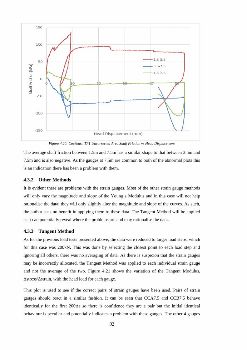
92
The average shaft friction between 1.5m and 7.5m has a similar shape to that between 3.5m and
7.5m and is also negative. As the gauges at 7.5m are common to both of the abnormal plots this
is an indication there has been a problem with them.
4.3.2 Other Methods
It is evident there are problems with the strain gauges. Most of the other strain gauge methods
will only vary the magnitude and slope of the Young’s Modulus and in this case will not help
rationalise the data; they will only slightly alter the magnitude and slope of the curves. As such,
the author sees no benefit in applying them to these data. The Tangent Method will be applied
as it can potentially reveal where the problems are and may rationalise the data.
4.3.3 Tangent Method
As for the previous load tests presented above, the data were reduced to larger load steps, which
for this case was 200kN. This was done by selecting the closest point to each load step and
ignoring all others, there was no averaging of data. As there is suspicion that the strain gauges
may be incorrectly allocated, the Tangent Method was applied to each individual strain gauge
and not the average of the two. Figure 4.21 shows the variation of the Tangent Modulus,
Δstress/Δstrain, with the head load for each gauge.
This plot is used to see if the correct pairs of strain gauges have been used. Pairs of strain
gauges should react in a similar fashion. It can be seen that CCA7.5 and CCB7.5 behave
identically for the first 200Δε so there is confidence they are a pair but the initial identical
behaviour is peculiar and potentially indicates a problem with these gauges. The other 4 gauges
Figure 4.20: Cockburn TP1 Uncorrected Area Shaft Friction vs Head Displacement

93
do not have as strong a correlation which is assumed to be a result of bending near the head of
the pile. Looking at the magnitudes of Δstress/Δstrain, it appears the gauges have been correctly
paired together. CCA3.5 and CCB3.5 have the higher initial Δstress/Δstrain which indicates
they are further down the pile.
Figure 4.22 shows the Δstress/Δstrain vs head load for the average of the strain gauge pairs. The
gauges at 7.5m are initially higher than the gauges at 3.5m but reduce to a constant
Δstress/Δstrain before the 3.5m pair. A pair of gauges that have not levelled off indicates that
load is still being developed above this point and as such a lower set of gauges should always
level off before a higher set. In this example it is not definitive that the 3.5m gauges and the
7.5m gauges have been mixed up but it does seem possible. This also makes sense in terms of
the magnitude of the strains as the 3.5m gauges have the lowest strain values throughout the
test.
If this is the case it is hoped that a simple analysis of the gauges with the 3.5m and 7.5m gauges
switched will provide a more logical interpretation of the data. This will be examined later in
the section.
Continuing with the Tangent Method Analysis Figure 4.23 shows the Δdstress/Δstrain vs strain
for the three gauge levels and the equivalent modulus from the secant method as well.
The secant modulus for the top strain gauges was:
𝐸 = −0.0068 . 𝜖 + 38
CCA7.5 and CCB 7.5B match
for the first 200µε
Figure 4.21: Cockburn TP1 Tangent Plot vs head load for all individual gauges
Equation 4.4
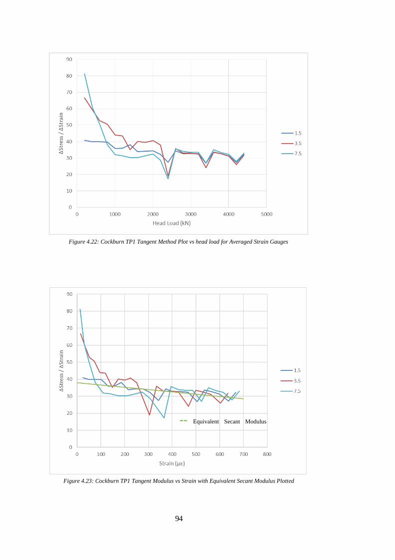
94
Figure 4.22: Cockburn TP1 Tangent Method Plot vs head load for Averaged Strain Gauges
Figure 4.23: Cockburn TP1 Tangent Modulus vs Strain with Equivalent Secant Modulus Plotted
-- Equivalent Secant Modulus
Line
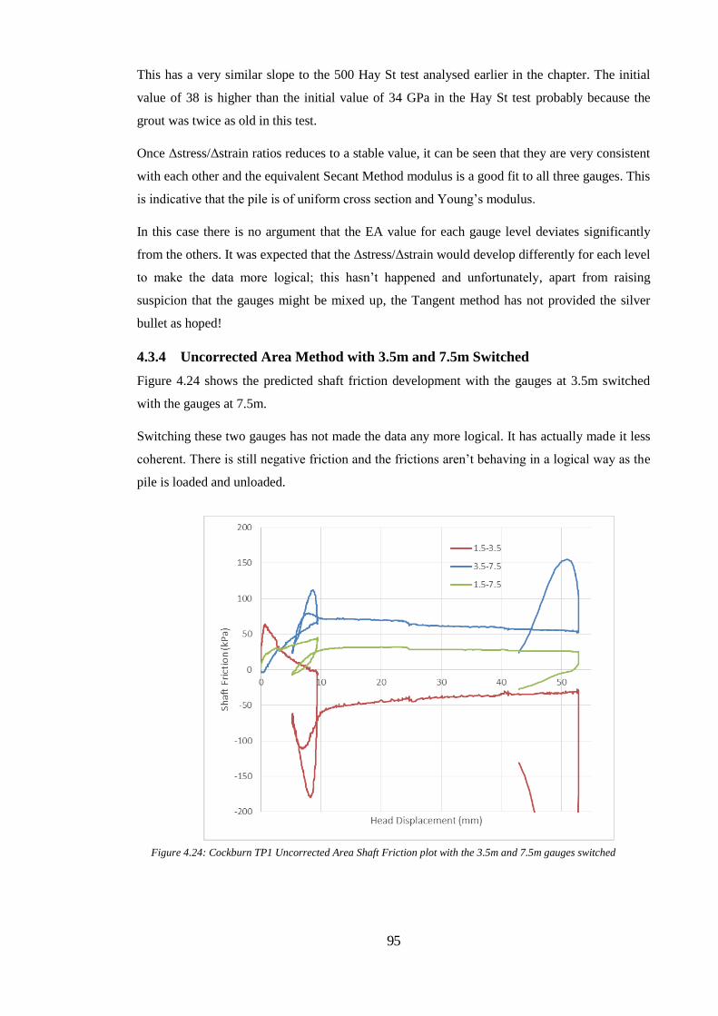
95
This has a very similar slope to the 500 Hay St test analysed earlier in the chapter. The initial
value of 38 is higher than the initial value of 34 GPa in the Hay St test probably because the
grout was twice as old in this test.
Once Δstress/Δstrain ratios reduces to a stable value, it can be seen that they are very consistent
with each other and the equivalent Secant Method modulus is a good fit to all three gauges. This
is indicative that the pile is of uniform cross section and Young’s modulus.
In this case there is no argument that the EA value for each gauge level deviates significantly
from the others. It was expected that the Δstress/Δstrain would develop differently for each level
to make the data more logical; this hasn’t happened and unfortunately, apart from raising
suspicion that the gauges might be mixed up, the Tangent method has not provided the silver
bullet as hoped!
4.3.4 Uncorrected Area Method with 3.5m and 7.5m Switched
Figure 4.24 shows the predicted shaft friction development with the gauges at 3.5m switched
with the gauges at 7.5m.
Switching these two gauges has not made the data any more logical. It has actually made it less
coherent. There is still negative friction and the frictions aren’t behaving in a logical way as the
pile is loaded and unloaded.
Figure 4.24: Cockburn TP1 Uncorrected Area Shaft Friction plot with the 3.5m and 7.5m gauges switched

96
The overall shaft friction between 1.5m and 7.5m is behaving in a more logical manner now but
is very low compared to normal expectations in this soil. These two strain gauge pairs have
always been the most logical however now we are assuming they are further apart which is
resulting in less stress.
The possible mix up of gauges seems unlikely as the data has not made any more sense and the
stress between 1.5m and 3.5m in the original interpretation is more likely that the very low
stress shown between 1.5m and 7.5m in Figure 4.24.
4.3.5 Summary
In this case the Tangent Method has not been able to rationalise the data as hoped but does lead
the author to believe that the problem is an electronic issue with the strain gauge system itself
rather than unusual pile geometry or soil conditions. In particular, it is the author’s opinion that
the lower strain gauges have serious issues and should be ignored. This makes the interpretation
of load distribution practically impossible.
There are too many problems with the strain gauge data from this test to provide reliable insights
into the pile’s behaviour.
This test has also highlighted that the strain gauge placement should be well documented with
photos and labels so that there can be no doubt about strain gauge levels.

97
Cockburn TP2 Strain Gauge Analysis
The strain gauge output is plotted on Figure 4.25 and is seen to be an improvement on TP1 e.g.
the lower pair of gauges at 7.5m have the lowest strain readings.
On a closer examination there are, however, a few discrepancies. The pair of gauges at 1.5m and
the pair at 3.5m have very similar readings throughout the test. This suggests minimal shaft
friction was developed over this 2.0m length of the pile. The low CPT resistances recorded in
this zone are consistent with low friction.
A larger concern is that, after the working load hold and unload, CCC3.5 does not recover strain
on the reload at the same rate as CCD3.5. What is interesting is that, throughout the final
loading, the gauge slowly recovers the strain until it is back to a similar value to CCD3.5. It is
also still gaining strain during load holds (see around the 6-hour mark) so the strain
development in the gauge is somewhat independent of the load. This indicates there is some
kind of instrument error or fixing issue with the gauge or creep effect.
Figure 4.26 shows what effect the delayed response of CCC3.5 has on the analysis; this plot
presents a simple uncorrected method analysis. For the first 10mm head displacement, the shaft
frictions are reasonable (when there was no delay apparent). After the pile is unloaded and
reloaded (head displacement ~10mm), the interpreted shaft friction in the top section of the pile
suddenly gains 100kPa and the lower section loses 70 kPa. These sudden gains and losses are
then largely reversed in steps as the test progresses. This is beyond any conventional
understanding of pile or soil behaviour and is not considered realistic. This is the direct result of
CCC3.5 significantly deviating from the response of the other gauges. The only conclusion that
can be drawn is that CCC3.5 has malfunctioned.
CCC3.5 has a delayed
response to the reload
Figure 4.25: Cockburn TP2 Strain vs Time

98
The question then is whether to include the other gauge at 3.5m (CCD3.5) in the analysis. It is
within the normally accepted 10 pile diameter range for bending effects so the reading of a
single strain gauge might not be representative of the overall strain at that level. As such,
including the single gauge at 3.5m could create a misleading interpretation of the test. The data
at 3.5m will therefore be ignored in the analysis of this test and is further evidence that the strain
gauge system used on this project needs examination before future implementation.
4.4.1 Uncorrected Area Method
No specific Modulus of Elasticity test was conducted for this pile and therefore a value 37GPa
will be used, as it was for TP1. This assumption produces the following results at maximum pile
load:
Load at 1.5m 6,296 kN Compared to a measured head load of 5,779kN
Load at 7.5m 5,063 kN
Table 4.14: Cockburn TP2 Uncorrected Area Interpretation
As the pile has an enlarged base a number of assumptions have to be made to calculate the base
response. As this Chapter is focusing on the interpretation of strain gauge data, only the load at
these two levels will be examined.
It can be seen that the pile head load is lower than the final load predicted at 1.5m. This type of
error is expected as this method assumes a constant Young’s Modulus.
The shaft friction vs head displacement has been plotted in Figure 4.27. It can be seen that the
average shaft friction increases right up to the final displacement of 50mm. As per the previous
analyses this is against the conventional shaft friction theory and is likely a result of the constant
Young’s Modulus assumption.
Figure 4.26: Cockburn TP2 Uncorrected Area Shaft Friction vs Head Displacement

99
What is also interesting on this plot is the significant negative friction calculated after unloading
from the working load. This is a significant amount of friction and points to a large locked in
load in the base. This is not unheard of in load tests but the magnitude of the negative friction is
greater than would be expected.
The first 20 kPa of shaft friction is very stiff and suggests that the soil has a certain amount of
cohesion to the pile shaft (noting that some degree of cementation might be anticipated from the
high qc values in the Cockburn sands).
4.4.2 Transformed Area Method
The test pile was reinforced with 8N32. Table 4.15 shows how the Transformed Area Modulus
is calculated.
Area of steel (mm2) 6,432
Area of Grout (mm2) 189,568
Equivalent Modulus 42.35 GPa
Table 4.15: Cockburn TP2 Transformed Area Modulus Calculation
As this pile is heavily reinforced (3.3% steel) the modulus has received a significant boost. The
results from the analysis are below. As a result of the higher modulus the loads are higher which
has led to further inaccuracy.
Table 4.16: Cockburn TP2 Transformed Area Interpretation
Load at 1.5m 7,151 kN Compared to a measured head load of 5,779kN
Load at 7.5m 5,716 kN
Figure 4.27: Cockburn TP2 Uncorrected Area Shaft Friction development

100
The shaft friction plot has not been included as it is identical to Figure 4.27 except that a factor
of 1.14 is applied (42.35 GPa / 37 GPa). Interpreted peak friction averaged over the full shaft
was 150 kPa.
4.4.3 Implicit Method
To utilise this method, it had to be assumed that the strain at 1.5m is equivalent to the strain at
the pile head. This will have the effect of ignoring the top 1.5m of the pile and will slightly
increase the calculated average shaft friction as it assumes there is less surface area. This
method produced the following results:
Load at 1.5m 5,779 kN Compared to a measured head load of 5,779kN
Load at 7.5m 4,647 kN
Table 4.17: Cockburn TP2 Implicit Method Interpretation
As expected this method predicts the pile head load exactly and has also resulted in a small
decrease in the predicted average shaft friction as can be seen in Figure 4.28.
This method has decreased the magnitude of the negative friction on the unload reload loop to a
more typical value.
4.4.4 Secant Modulus Method
As with the implicit method it is necessary to make the assumption that the strain in the gauge at
1.5m is equivalent to the strain at the pile head.
This method calculated that the modulus had the following relationship:
𝐸 = −0.0063 . 휀 + 39.229
Figure 4.28: Cockburn TP2 Implicit Method Shaft Friction Development
Equation 4.5

101
This plot can be seen in Figure 4.29 and was calculated using a polynomial trend line in
Microsoft Excel. This trend line had an R2 value of 0.9999 so was a good fit with the data.
This modulus equation compares well to the one calculated in the 500 Hay St Test. That test had
a similar slope of -0.0071 and an initial modulus of 34.473. As the grout in this test was twice
the age of the 500 Hay St Test a higher modulus is expected. Slopes and intercepts comparable
to other data increase the confidence in the reliability of the gauges.
Using this relationship at each gauge location has produced the following results at maximum
pile load.
Load at 1.5m 5,747 kN Compared to a measured head load of 5,779kN
Load at 7.5m 4,767 kN
Table 4.18: Cockburn TP2 Secant Method Interpretation
This method has produced another drop in the shaft friction down to 103 kPa and the predicted
friction reaches a stable ultimate value, as expected in this material. The negative friction, on
unloading, is 40 kPa in this case.
Figure 4.29: Secant Modulus Top Strain Gauge trendline

102
4.4.5 Tangent Method
As for the previous tests, it was found necessary to reduce the data to 250 kN steps. Figure 4.31
shows the plot of strain vs Δstress/Δstrain. It can be seen that the gauges have a good correlation
which only varies slightly at the load holds. The gauges at 7.5m are initially high and reduce
down to similar values to the 1.5m gauges as the test progresses, which is in line with
expectations.
The trendline calculated for the gauges at 1.5m can be converted to an equivalent Secant
Modulus of:
𝐸 = −0.0062 . 휀 + 39.647
Figure 4.30: Cockburn TP2 Secant Method Shaft Friction Development
Equation 4.6
Figure 4.31: Cockburn TP2 Tangent Method Plot

103
This is very close to the Secant Modulus that was calculated above which gives confidence in
the relationship.
Working out the trendline for the gauge at 7.5m isn’t as simple. As only the points past the peak
shaft friction should be taken into account, we need to look at the shaft friction plots worked out
in prior methods. The most reliable plot will be the Secant Method plot (Figure 4.30) which
shows that the rate of development of shaft friction is low past 20mm head displacement. This is
equivalent to a strain of 450 µε. As can be seen below in Figure 4.32(a) the data have been
isolated to this range. Unfortunately, as the pile was only loaded to 50mm displacement there
are not a lot of data points and there was a few short load holds that have created noise in the
plots. It is not possible to get a decisive slope from the data alone, so the equivalent data from
the 1.5m gauges has been isolated with the trendline drawn so that a comparative line can be
drawn (Figure 4.31 (a)). It is obvious that the Tangent modulus at 7.5m is higher than at 1.5m
but by how much isn’t clear. As can be seen, the line drawn has the same slope and intersects
the peak at approximately the same point. This is as reliable as can be obtained for this test.
The Tangent modulus equation for the gauges at 7.5m is:
∆𝑠𝑡𝑟𝑒𝑠𝑠
∆𝑠𝑡𝑟𝑎𝑖𝑛= −0.0124 . 휀 + 41
And the equivalent Secant modulus equation is:
𝐸 = −0.0062 . 휀 + 41
Using these two Secant moduli for the data gives the following loads at 50mm displacement:
Load at 1.5m 5,833 kN Compared to a measured head load of 5,779kN
Load at 7.5m 5,019kN
Table 4.19: Cockburn TP2 Tangent Method Interpretation
Equation 4.7
Equation 4.8
Figure 4.32 Cockburn TP2 Tangent Method Trendlines (a) 1.5m (b) 7.5m
1.5m 7.5m

104
The average shaft friction between 1.5m and 7.5m has been plotted on Figure 4.32 against head
displacement.
The peak shaft friction is now 86 kPa, which is the smallest value from all previous analyses. It
also flattens off after 20mm settlement as is generally expected. This builds confidence that this
is the most reliable calculation of shaft friction for this test. However, the negative friction of 40
kPa is higher than generally anticipated.
4.4.6 Comparison
Figure 4.33 compares the results of the methods described above for TP2. In line with the analysis
of previous tests, it was found that the uncorrected area and transformed area methods are the
least reliable as they don’t utilise the data available to make corrections to the modulus values.
The implicit method is a convenient method to calculate the stresses in the pile and produced an
interpretation close to the secant method with less work. The correlation seen during the secant
method gives confidence that the method is providing a reliable interpretation of the load
distribution but in this case it has shown its weakness, being sensitive to changes in the EA value
at each gauge level. Despite being difficult to interpret the Tangent Method has picked up these
changes and produced a shaft friction plot that is in line with expected behaviour.
Figure 4.33: Cockburn TP2 Tangent Method Shaft Friction Development

105
Figure 4.34: Cockburn TP2 Comparison of Interpretations

106
Chapter 5
Pile Performance Parameter Selection

107
5 Pile Performance Parameter Selection
500 Hay St Pile Parameters
This test was detailed in Chapter 3 and the strain gauges were analysed in Chapter 4. The
Tangent Method Analysis produced an interpretation of the distributed loads down the pile in
which there is a high degree of confidence in. Using Figure 4.9, which shows the shaft friction
vs head displacement plots of the different pile sections, this test will be back analysed using
RATZ to develop a model that can applied to other load tests. It is hoped to gain a better
understanding of the shear modulus, peak friction and base capacity values used in RATZ when
analysing bored piles in Perth sands.
5.1.1 Corrections for Axial Compression for Segment Analyses
Using shaft friction curves from Figure 4.9, the test pile will be split into segments as shown in
Figure 5.1 which will then be separately analysed using RATZ to obtain the best match. As
Figure 4.9 was only used for broad comparison it plotted shaft friction against head
displacement. As the pile segments will be analysed individually each section will need to be
corrected for the axial compression of the segments above it. This will be done according to the
following simplified approach.
Strain is defined as:
휀 = ∆𝐿
𝐿
Therefore, the axial compression correction will be:
∆𝐿 = 휀 . 𝐿
Applying this to each segment requires an assumption to be made about what the average strain
is over this segment. It will be assumed that the average strain over the segment will be the
mean of the strain at the top and bottom of the segment. The correction at the top of a segment
will be the sum of the corrections above it. For example, the correction at the top of the segment
between 3.0m and 6.0m will be:
∆𝐿0.5−3.0 = ∆𝐿0−0.5 + 휀0.5 + 휀3.0
2 . 𝐿0.5−3.0
A summary of this is shown in Figure 5.1.
Equation 5.2
Equation 5.1
Equation 5.3

108
Figure 5.1: 500 Hay St Axial Compression Corrections for pile segment analyses
Applying these corrections to Figure 4.9 produces the curves seen in Figure 5.2. For comparison,
the original shaft friction vs head displacement curves have been left on. As expected, the
correction is insignificant for the upper section and then increases through each segment until the
correction is approx. 5mm over the 10 – 13.5m segment at Rug.
Depth Strain Correction
0.0 ε0 (≈ ε0.5)
0.5 ε0.5 ∆𝐿0−0.5 =
휀0 + 휀0.5
2 . 𝐿0−0.5
3.0 ε3.0 ∆𝐿0.5−3.0 = ∆𝐿0−0.5 +
휀0.5 + 휀3.0
2 . 𝐿0.5−3.0
6.0 ε6.0 ∆𝐿3.0−6.0 = ∆𝐿0.5−3.0 +
휀3.0 + 휀6.0
2 . 𝐿3.0−6.0
10.0 ε10.0 ∆𝐿6.0−10.0 = ∆𝐿3.0−6.0 +
휀6.0 + 휀10.0
2 . 𝐿6.0−10.0
13.5 ε13.5 ∆𝐿10.0−13.5 = ∆𝐿6.0−10.0 +
휀10.0 + 휀13.5
2 . 𝐿10.0−13.5

109
This plot was then normalised by the peak shaft friction to examine the form of the normalised
relationship; see Figure 5.3. The shaft friction between 0.5m and 3.0m appears to be behaving
strangely. This has a much smaller τp than the other gauges so small errors have been magnified
by the normalisation. As can be seen in Figure 5.2 these are only variations of a few kPa which
are not unexpected when analysing strain gauges. The development of shaft friction in the upper
three segments closely match when normalised. This is suggesting that the peak shaft friction
and shear modulus are related. The lower segment behaves noticeably differently from the other
segments which suggests there are some other factors contributing to the shear modulus. This
will be discussed later in this section.
Each segment will now be examined individually in RATZ in order to determine the best fit
parameters.
Figure 5.2: 500 Hay St Corrected Shaft Friction vs Displacement

110
5.1.2 Modelling Individual Segments Shaft Response in RATZ
To model the shaft friction of individual segments in RATZ the base response is set to zero and
the pile is modelled as the length of the segment (ie 3m long). The Young’s Modulus of the pile
was set at 38GPa as this is a typical value seen on the tests. Using short segments, the Young’s
Modulus won’t make a significant difference so this simplification is acceptable. The only other
parameter that can affect the load transfer curve is the load transfer parameter (ζ)). This
parameter determines the initial slope of the load transfer curve (k):
𝑘 = 𝐺
휁
Because of this direct relationship, changing either G or ζ will change the initial slope of the
load transfer curve. It is therefore unnecessary to change ζ as any change in G will have the
same effect. As such only G and ξ will be altered to alter the curve predicted by RATZ.
0.5 to 3.0
This segment experienced a peak shaft friction of 20 kPa. As mentioned previously the noise is
a relatively large part of this and has made the shaft friction curve appear strange. Figure 5.4
below plots the test result against various curves that have been produced using RATZ; G has
been varied between 4000kPa, 8000kPa and 12000kPa whilst ξ (xi) has also been alternated
between 0 and 0.3 to see what effect it has.
Equation 5.4
Figure 5.3: Normalised Corrected Shaft Friction vs Displacement

111
No ideal model has been found that matched the curve perfectly. The parabolic solution that
RATZ adopts is evidently not very suitable. There is no option when using RATZ other than to
compromise and pick a G value that best represents the curve.
A G of 4000kPa is too low as it is under the test data nearly the whole way up to peak friction.
On the other hand, a G of 12000kPa is good for the first few millimetres but becomes too steep
after that. A G of 8000kPa provides a good compromise and is the best of the three moduli
represented here.
ξ has not helped model the curve any better; in fact, it has the opposite effect of straightening
out the curve and making the non-linear portion change slope more dramatically.
It should be noted that for clarity only the test data up to 30mm is shown; the test data return to
20kPa by 60mm.
3.0m to 6.0m
This segment experienced a peak shaft friction of 70 kPa and the noise seen in the first segment
is also present but is not as pronounced as it is a smaller proportion of the peak friction. Figure
5.5 plots the test result against various curves that have been produced using RATZ. G has been
varied between 7500kPa, 15000kPa and 22500kPa whilst ξ (xi) has also been alternated
between 0 and 0.3 to see what effect it has.
Figure 5.4: RATZ models plotted against test data for segment between 0.5m and 3.0m

112
As for the first segment, no ideal model has been found that matched the curve perfectly. The
parabolic curve does not fit the response of this sand very well and a compromise needs to be
found when choosing G.
A G of 7500kPa is too low as it is under the test data nearly the whole way up to peak friction.
On the other hand, a G of 22500kPa is good for the first 5 millimetres but overtakes the shaft
friction after that. A G of 1500kPa underestimates the first part of the curve but gives an
improved match in the 6-10mm range which is a typical working load range for a pile.
Again ξ has not helped model the curve any better and ξ = 0 provides better matches. It seems to
be having a similar effect to an increased shear modulus.
6.0m to 10.0m
The segment between 6m and 10m has a peak shaft friction of 105 kPa. As seen in Figure 5.6
this segment has had the stiffest response so a larger shear modulus should be expected. The
shear modulus was varied between 18 MPa and 32 MPa, whilst ξ (xi) has also been alternated
between 0 and 0.3 to see what effect it has.
Again RATZ has not been able to model the non-linear development of shaft friction very well
and there is no ideal shear modulus. A shear modulus of 18000 kPa under predicts the shaft
friction over the majority of the development and 32000 kPa is a closer match to the pre 5mm
zone but over-predicts the curve after 5mm displacement; 25000 kPa has been chosen as a
compromise best-fit.
Figure 5.5: RATZ models plotted against test data for segment between 3.0m and 6.0m

113
10.0m to 13.5m
The segment between 10m and 13.5m has a peak shaft friction of 136 kPa. The development of
shaft friction in this zone was noticeably different from the other segments. The first 40 kPa of
friction is very stiff and is indicative of cohesion in this zone of soil. The shear modulus has
been varied between 18 MPa and 32MPa whilst ξ (xi) has also been alternated between 0 and
0.3 to see what effect it has.
Again RATZ has not been able to model the non-linear development of shaft friction well and
this segment in noticeably worse than the others. A shear modulus of 18000 kPa under predicts
the shaft friction over the first half of the curve but is a good match for the latter half of the
curve. 32000 kPa is a closer match to the pre 5mm zone but over predicts the curve after 5mm
displacement; 25000 kPa has been chosen as a compromise best-fit.
.
Figure 5.6: RATZ models plotted against test data for segment between 6.0m and 10.0m

114
5.1.3 Overall Shaft Friction Response
The best-fit G values for each segment are now used in a RATZ analysis of the shaft responses
shown in Figure 5.8. The parameters in Table 5.1 were employed for the analysis.
Depth (m) τp (kPa) G (kPa)
0.5 – 3.0 20 8,000
3.0 – 6.0 70 15,000
6.0 – 10 105 25,000
10 – 13.5 136 18,000
Table 5.1: Parameters Used to Model Average Shaft Friction 0.5-13.5
By looking at each segment individually we get a RATZ prediction which is reasonably close to
the measured value. In line with the compromise made when choosing the G values, RATZ is
seen on Figure 5.8 to under-predict the shaft friction at lower displacements and over predict
shaft friction at higher displacements until τp is developed.
Figure 5.7: RATZ models plotted against test data for segment between 10.0m and 13.5m
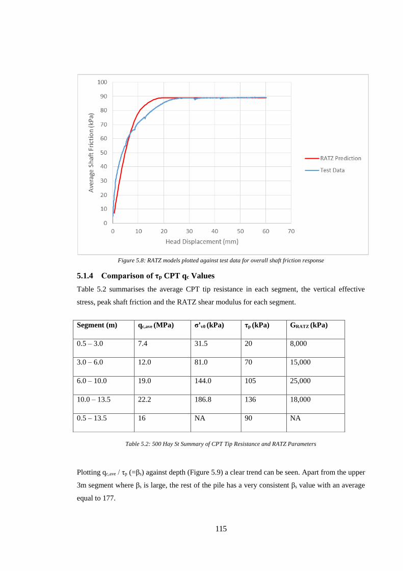
115
5.1.4 Comparison of τp CPT qc Values
Table 5.2 summarises the average CPT tip resistance in each segment, the vertical effective
stress, peak shaft friction and the RATZ shear modulus for each segment.
Table 5.2: 500 Hay St Summary of CPT Tip Resistance and RATZ Parameters
Plotting qc,ave / τp (=βs) against depth (Figure 5.9) a clear trend can be seen. Apart from the upper
3m segment where βs is large, the rest of the pile has a very consistent βs value with an average
equal to 177.
Segment (m) qc,ave (MPa) σ'v0 (kPa) τp (kPa) GRATZ (kPa)
0.5 – 3.0 7.4 31.5 20 8,000
3.0 – 6.0 12.0 81.0 70 15,000
6.0 – 10.0 19.0 144.0 105 25,000
10.0 – 13.5 22.2 186.8 136 18,000
0.5 – 13.5 16 NA 90 NA
Figure 5.8: RATZ models plotted against test data for overall shaft friction response

116
5.1.5 Comparison of GRATZ CPT qc Values
Figure 5.10 plots the GRATZ values used in pile test interpretation against the average qc in that
segment. A linear trend line has then been applied to the points with ±20% interval lines.
Figure 5.9: 500 Hay St β vs Depth
Figure 5.10: 500 Hay St qc vs GRATZ

117
In the top three segments there is a strong linear relationship where G ≈1.25qc however the
segment between 10.0m and 13.5m is an outlier from this relationship where G ≈ 0.8qc.
Comparing this to the CPT plots and specifically looking at the friction ratio there is a distinct
change in the material at a depth of approx. 8.75m, see Figure 5.11. This coincides with the
water table level and the material is behaving differently from this point. This behavioural
change will affect the shaft friction behaviour of the pile. Despite a drop in the friction sleeve
reading the peak shaft friction has not reduced but has increased. This is indicating that the
material below this level has a degree of cementation which is in line with the shaft friction plot
in the 10.0m to 13.5m segment.
Overall this test indicates that G ≈ qc. In line with other correlations for soil stiffness, this
relationship should be considered approximate.
Figure 5.12 compares GRATZ to the vertical effective stress (σ’v0). There is an increase of GRATZ
with increasing stress but the relationship isn’t as strong as the correlation with qc. Again the
upper segments have a very strong linear correlation with σ’v0 but the segment between 10.0m
and 13.5m does not fit in with this relationship, as the r2 values show there is stronger link
between GRATZ and qc than σ’v0.
In line with other suggested correlations for soil stiffness, GRATZ has been compared to σ’v00.33.
qc0.33 . pATM
0.33 in Figure 5.13 (where patm is atmospheric pressure = 100 kPa). Overall this is
similar to the previous two plots but the r2 value of 0.66 indicates that this is an improvement
over just looking at qc which had an r2 value of 0.60.
Figure 5.11: 500 Hay St CPT plots with friction sleeve and friction ratio data
Abrupt change in Fr
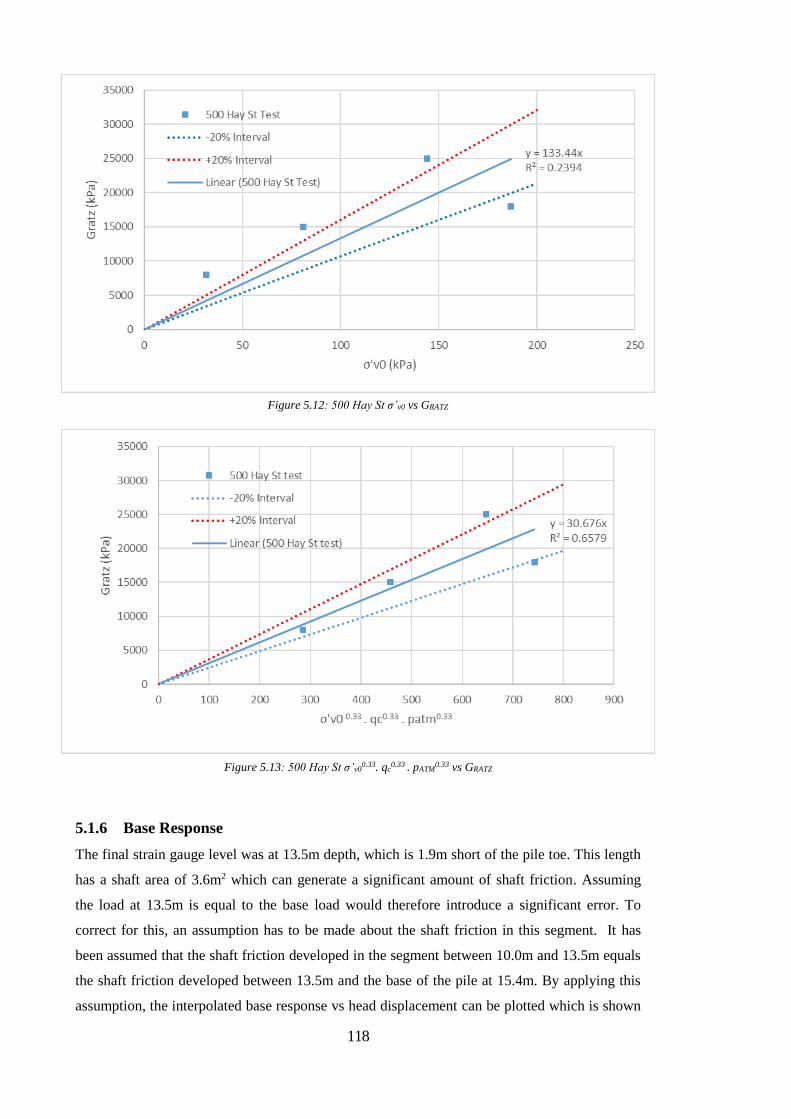
118
5.1.6 Base Response
The final strain gauge level was at 13.5m depth, which is 1.9m short of the pile toe. This length
has a shaft area of 3.6m2 which can generate a significant amount of shaft friction. Assuming
the load at 13.5m is equal to the base load would therefore introduce a significant error. To
correct for this, an assumption has to be made about the shaft friction in this segment. It has
been assumed that the shaft friction developed in the segment between 10.0m and 13.5m equals
the shaft friction developed between 13.5m and the base of the pile at 15.4m. By applying this
assumption, the interpolated base response vs head displacement can be plotted which is shown
Figure 5.13: 500 Hay St σ’v00.33. qc
0.33 . pATM0.33 vs GRATZ
Figure 5.12: 500 Hay St σ’v0 vs GRATZ

119
in Figure 5.14. Also as shown in Figure 5.14 is the base responses vs estimated base
displacement. This has been calculated in the same manner as the corrections used for the shaft.
It is clear that the base pressure is still increasing past 60mm (0.1D). This is expected for a
bored pile in sand. It can be seen that the slope of the base pressure starts to reduce but it could
actually be modelled reasonably well using a linear equation up to 0.1D. A best-fit polynomial
trend line (power 2, parabolic) has also been fitted (as can be applied in RATZ) and gives a
reasonable match to the measured response.
As discussed in Chapter 2, RATZ requires two inputs to calculate the base response; the
ultimate end bearing pressure at pile base (qb) and the displacement to mobilise this pressure
=wb. In this case specifying 60mm as wb would not model the interpolated base response
accurately. Larger values of qb and wb would need to be used.
A RATZ model was setup to model the base response assuming a parabolic response. The pile
was 0.2m long, had 0.1 kPa of shaft friction and a concrete modulus of 38 GPa. Various values
of wb were applied to see what quality of match was achieved. Once a wb was inputted, the qb
was varied until the same load at 55mm displacement was achieved (2,027kN). Figure 5.15
shows the computed trends wb of 0.1D, 0.2D and 0.4D. It should be noted that in this case the
measured data have been corrected for axial compression of the pile.
Figure 5.14: 500 Hay St Pile Base Response
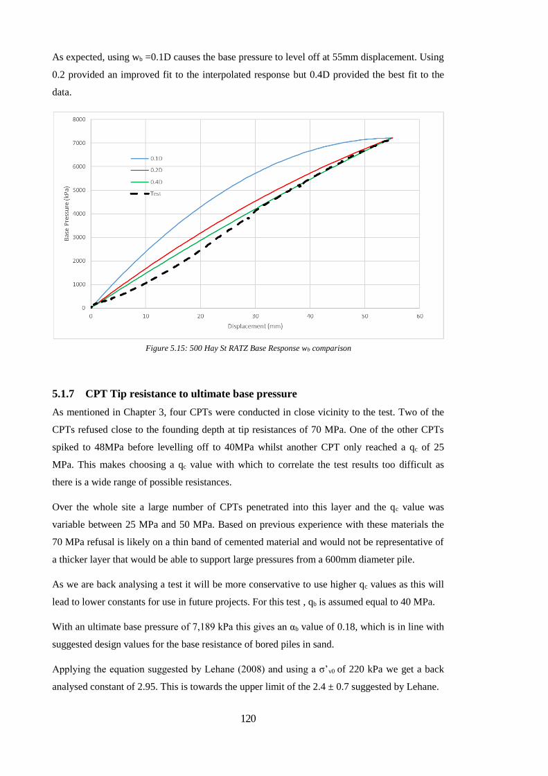
120
As expected, using wb =0.1D causes the base pressure to level off at 55mm displacement. Using
0.2 provided an improved fit to the interpolated response but 0.4D provided the best fit to the
data.
5.1.7 CPT Tip resistance to ultimate base pressure
As mentioned in Chapter 3, four CPTs were conducted in close vicinity to the test. Two of the
CPTs refused close to the founding depth at tip resistances of 70 MPa. One of the other CPTs
spiked to 48MPa before levelling off to 40MPa whilst another CPT only reached a qc of 25
MPa. This makes choosing a qc value with which to correlate the test results too difficult as
there is a wide range of possible resistances.
Over the whole site a large number of CPTs penetrated into this layer and the qc value was
variable between 25 MPa and 50 MPa. Based on previous experience with these materials the
70 MPa refusal is likely on a thin band of cemented material and would not be representative of
a thicker layer that would be able to support large pressures from a 600mm diameter pile.
As we are back analysing a test it will be more conservative to use higher qc values as this will
lead to lower constants for use in future projects. For this test , qb is assumed equal to 40 MPa.
With an ultimate base pressure of 7,189 kPa this gives an αb value of 0.18, which is in line with
suggested design values for the base resistance of bored piles in sand.
Applying the equation suggested by Lehane (2008) and using a σ’v0 of 220 kPa we get a back
analysed constant of 2.95. This is towards the upper limit of the 2.4 ± 0.7 suggested by Lehane.
Figure 5.15: 500 Hay St RATZ Base Response wb comparison

121
It is noted that if a qb of 70 MPa is used instead of 40 MPa then a constant of 2.23 is obtained
and if a qb of 25 MPa is used then we get a constant of 3.73. Because of this uncertainty it is
always best to apply the more conservative numbers to future piles so it is hard to disagree with
Lehane’s suggested average of 2.4.
5.1.8 Overall Pile RATZ Model
Combining the shaft and base models described above produces Figure 5.16 which compares
the combined model to the measured pile head response. Through the analysis of each segment
a RATZ model that closely fits the observed test data has been achieved. The difficulty of
matching the shaft friction data is still evident. Without adjusting the program’s shaft response
curve equations this is as good as it will get whilst staying consistent with the evidence
produced by the strain gauges.
Figure 5.16: 500 Hay St Test t-z Curve vs RATZ model

122
Application to Other Tests
Taking what we have observed in the 500 Hay St test it can then be applied to other load tests
where there has been no strain gauge data. The following relationships will be applied to the
CPT data and then the RATZ output will be compared to the load test data.
Parameter Inputs Relationship
τp qc τp = qc / 175
GRATZ qc, σ'v0 GRATZ = 30.6qc0.33 .σ'v0
0.33 . pATM0.33
qb,0.1D qc, σ'v0 qb,0.1D = 2.4 .qc0.5 . σ'v0
0.25 pATM0.25
w Db 0.4 . Db
Table 5.3: RATZ Parameters Applied to Other Tests
5.2.1 UWA Load Test TP1, Crawley WA
This test was described in Chapter 3. Using the CPT and the parameters described above we get
Figure 5.17 which compares the results to the test data.
The RUG has been slightly over predicted but is within a range any pile designer would be happy
with. However, the stiffness of the pile at working load has been significantly over predicted. At
the working load of 1200kN the RATZ model predicts ~5mm movement whilst the test
recorded over 10mm. In reality 10mm settlement at working loads is still considered OK when
applied to a building core. This error in stiffness can significantly alter the distribution of loads.
Figure 5.17: UWA TP1 Test vs RATZ Model
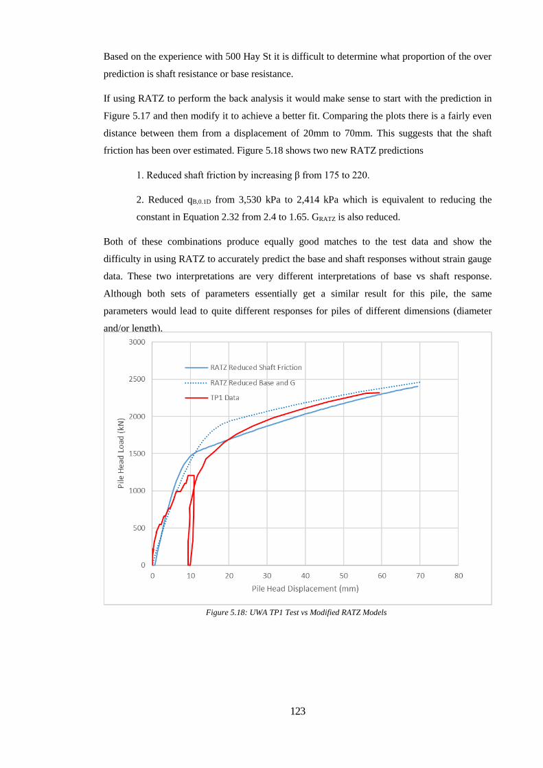
123
Based on the experience with 500 Hay St it is difficult to determine what proportion of the over
prediction is shaft resistance or base resistance.
If using RATZ to perform the back analysis it would make sense to start with the prediction in
Figure 5.17 and then modify it to achieve a better fit. Comparing the plots there is a fairly even
distance between them from a displacement of 20mm to 70mm. This suggests that the shaft
friction has been over estimated. Figure 5.18 shows two new RATZ predictions
1. Reduced shaft friction by increasing β from 175 to 220.
2. Reduced qB,0.1D from 3,530 kPa to 2,414 kPa which is equivalent to reducing the
constant in Equation 2.32 from 2.4 to 1.65. GRATZ is also reduced.
Both of these combinations produce equally good matches to the test data and show the
difficulty in using RATZ to accurately predict the base and shaft responses without strain gauge
data. These two interpretations are very different interpretations of base vs shaft response.
Although both sets of parameters essentially get a similar result for this pile, the same
parameters would lead to quite different responses for piles of different dimensions (diameter
and/or length).
Figure 5.18: UWA TP1 Test vs Modified RATZ Models
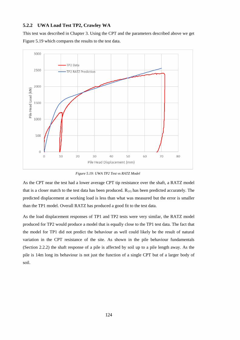
124
5.2.2 UWA Load Test TP2, Crawley WA
This test was described in Chapter 3. Using the CPT and the parameters described above we get
Figure 5.19 which compares the results to the test data.
As the CPT near the test had a lower average CPT tip resistance over the shaft, a RATZ model
that is a closer match to the test data has been produced. RUG has been predicted accurately. The
predicted displacement at working load is less than what was measured but the error is smaller
than the TP1 model. Overall RATZ has produced a good fit to the test data.
As the load displacement responses of TP1 and TP2 tests were very similar, the RATZ model
produced for TP2 would produce a model that is equally close to the TP1 test data. The fact that
the model for TP1 did not predict the behaviour as well could likely be the result of natural
variation in the CPT resistance of the site. As shown in the pile behaviour fundamentals
(Section 2.2.2) the shaft response of a pile is affected by soil up to a pile length away. As the
pile is 14m long its behaviour is not just the function of a single CPT but of a larger body of
soil.
Figure 5.19: UWA TP2 Test vs RATZ Model
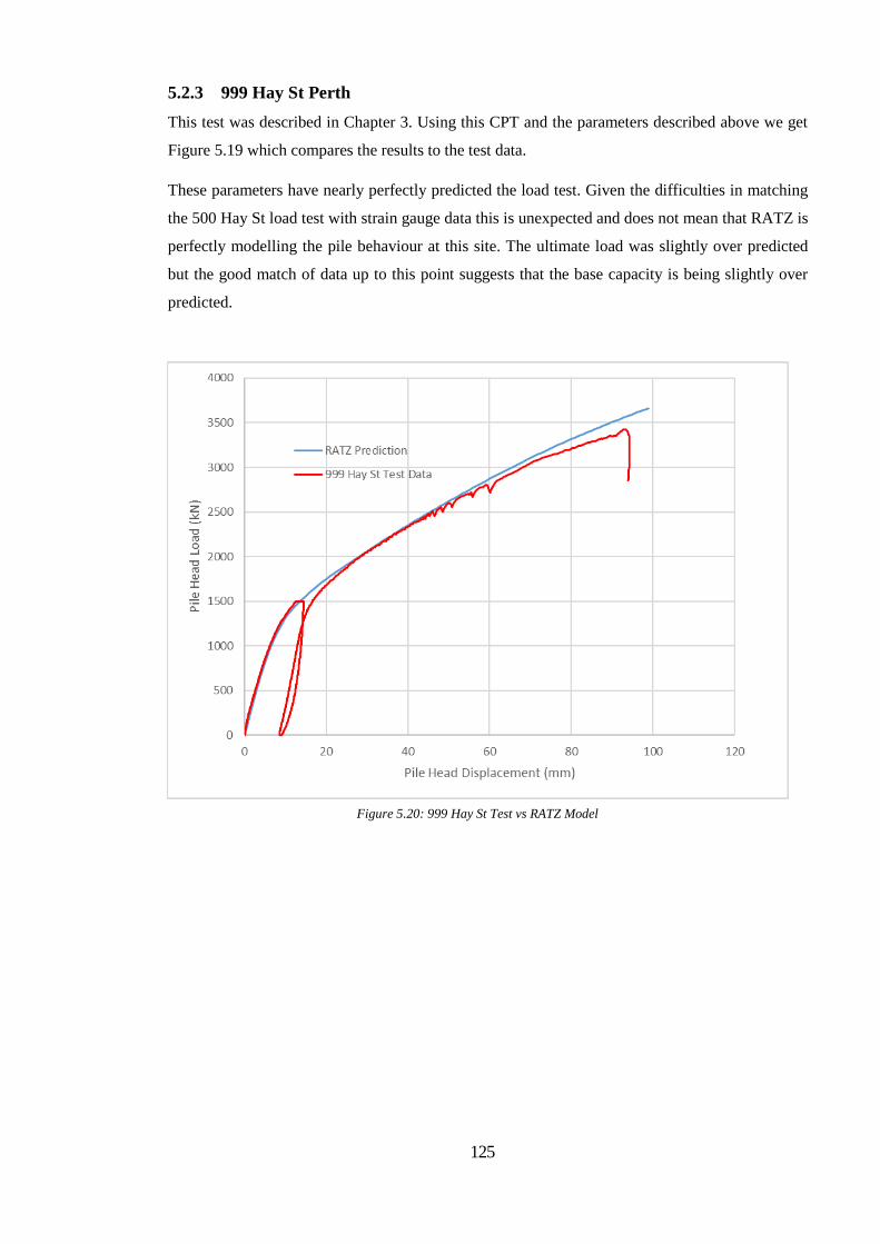
125
5.2.3 999 Hay St Perth
This test was described in Chapter 3. Using this CPT and the parameters described above we get
Figure 5.19 which compares the results to the test data.
These parameters have nearly perfectly predicted the load test. Given the difficulties in matching
the 500 Hay St load test with strain gauge data this is unexpected and does not mean that RATZ is
perfectly modelling the pile behaviour at this site. The ultimate load was slightly over predicted
but the good match of data up to this point suggests that the base capacity is being slightly over
predicted.
Figure 5.20: 999 Hay St Test vs RATZ Model

126
Chapter 6
Conclusions

127
6 Conclusions
Determination of load distribution from strain gauge data
From these load tests and their subsequent analysis, it has been found that:
1. Determining the distribution of load in bored piles using strain gauges is not as
straightforward as is often believed
2. Although the Uncorrected Area and Transformed Area Methods are the least accurate, they
are very easy to apply to get quick estimates and hence allow quick checks of the accuracy of
strain gauge data. Their simplicity leads them to be most applicable to analysing ‘live’ data as
the test is progressing. The strain gauges can be quickly checked to see if they are responding as
expected or reveal if there are possible problems.
3. The Implicit Method is simple to apply and gives a somewhat ‘calibrated’ interpretation of
the pile’s response. It is a useful baseline for the rest of the analysis methods as it requires
practically no interpretation by the data analyser.
4. The Secant Method has been shown to further refine the strain gauge analysis by taking the
strain dependency of the Young’s Modulus into account. It requires a certain degree of
processing of the data so is not possible in the field during a test.
5. As shown by the 500 Hay St test the Tangent Method provides the most in depth information
on the pile test but it is far more difficult to apply than all other methods. From these tests it is
the author’s opinion that the recommendations by Fellenius (1989,2001) are better described as
pre-requisites. Without meeting these criteria, it is difficult to apply the Tangent Method. These
are reiterated below:
i) The pile should be loaded at a constant load rate and not have any load holds or
unloads. The test designer will need to decide what is more important; increasing
confidence in the distribution of load along the pile or measurement of pile creep at
working loads
ii) If a load hold is necessary unload reload loops should still be avoided. These unload
reload loops have shown to hinder the Tangent method analysis by creating large
distortions in the Δstress / Δstrain values.
iii) The test frame needs to have excess capacity so that the pile can be sufficiently loaded
to exceed peak shaft friction by as much as possible. The more data there are past this
point the more reliable the analysis will be. In addition if capacity is still being developed
past a displacement of 0.1D then the test should continue for as long as possible.
128
6. It was found that the methods are complementary to each other. Applying one type of
analysis can help confirm assumptions made in another. The author has found that applying all
the methods in a progressive manner gives greater overall confidence in the analysis.
Correlating pile performance to CPT results
Based on the static load tests examined in this study the following conclusions were made in
regards to predicting a pile load deformation response from CPT results.
1. In this case RATZ has not been able to model the shaft friction response of the piles as well
as hoped. This is a result of the simplifications required to make a reasonably user friendly
program.
2. As a result of this, using RATZ to obtain perfect fits will lead to erroneous results.
3. The relationships that Lehane (2009) determined between shaft friction, base capacity and
CPT tip resistance for bored piles in sand are generally supported by this study.
𝑞𝐵,0.1𝐷 = (2.4 ± 0.7). 𝑞𝑐 0.5 . 𝜎𝑣0
′ 0.25 . 𝑝𝐴𝑇𝑀 0.25
𝛽𝑠 ≅ 175
It should be noted that this is a small set of tests so more generalised correlations are not
possible.
4. In line with these load tests and expected behaviour bored piles in sand, there was no
plunging type failure at 0.1D, the base pressure continues to gain load past this point. These
tests showed that when using RATZ to predict a bored pile in sands load deformation it is more
appropriate to use an equivalent base pressure at a larger displacement. 0.4 D was found to be
appropriate for these tests.
4. Despite the limitations with RATZ described above GRATZ for a bored pile in sand appears to
be best related to the CPT tip resistance by:
GRATZ ≈ 30.6 . qc0.33 .σ'v0
0.33 . pATM0.33
It is important to note that this is based on the back analysis of one load test and then examined
against 3 other tests where it showed some predictive potential. This relationship will require
further confirmation with other static load tests with high quality data.

129
7 References
Baguelin, F., & Franl, R. (1979). Theoretical studies of piles using the finite element method.
International Conference on Numerical Methods in Offshore Piling (pp. 33-91).
London: ICE.
Baldi, G., Bellotti, R., Ghionna, V. H., Jamiokowski, M., & Lo Presti, D. C. (1989). Modulus of
sands from CPTs and DMTs. Proc. 12th Int. Conf. on SMFE Vol. 1 (pp. 165-170). rio
de Janeiro: Balkema, Rotterdam.
Baldi, G., Bruzzi, D., Superbo, S., Battaglio, M., & Jamiolkowski, M. (1986). Interpretation of
CPTs and CPTUs; 2nd part: drained penetration of sands. Proceedings of the Fourth
International Geotechnical Seminar, (pp. 143-156). Singapore.
Comimitee BD-002, Concrete Structures. (2009). AS 3600 - Concrete Strucutres. Sydney:
Australian Standards.
Committee CE-018, Piling. (2009). AS 2159 - Piling - Design and installation. Sydney:
Standards Australia.
Cundall, P. A., & Stack, O. D. (1979). A discrete numerical model for granular assemblies.
Geotechnique Vol 29, 47-66.
De Cock, F., Legrand, C., & Huybrechts, N. (2003). Overview of design methods of axially
loaded piles in Europe - Report of ERTC3-Piles. Proceedings 8th European Conference
on Soil Mechanics and Geotechnical Engineering, (pp. 663-715). Prague.
Fahey, M., Lehane, B. M., & Stewart, D. (2003). Soil stiffness for shallow foundaiton design in
the Perth CBD. Australian Geomechanics VOl 38 No 3 Spetember 2003, 61-90.
Fahey, M., Schneider, J. A., & M, L. B. (2007). Self-boring pressuremeter testing in Spearwood
Dune Sand. Australian Geomechanics Vol 42 No. 4 December, 57-72.
Fellenius, B. H. (1989). Tangent modulus of piles determined from strain data. Proceedings of
the 1989 Foundation Engineering Congress (pp. 500-510). Evanston: ASCE.
Fellenius, B. H. (2001). From strain measurments to load in an instrumented pile. Geotechnical
News, pp. 19(1): 35-38.
Fleming, W. G., J, W. A., Randolph, M. F., & Elson, W. K. (1985). Piling Engineering.
Glasgow: Surrey University Press.
Hyett, A. J., & Bawden, W. F. (1992). Physical and mechanical properties of normal portland
cement pertaining to fully grouted cable bolts. Proceedings of International Symposium
on ground support and 16th Canadian rock mechanics conference. Sudbury, Canada.

130
ISSMFE. (1989). International reference test procedure for cone penetration test (CPT).
Linkoping: Swedish Geotechnical Institute.
Lam, C., & Jefferis, S. A. (2011). Critical assessment of pile modulus determination methods.
Canadian Geotechnical Journal Vol 48, 1433-1448.
Lee, J. H., & Salgado, R. (1999). Determination of pile base resistance in sands. Journal of
Geotechnical and Geoenvironmental Engineering, ASCE, 673-683.
Lehane, B. M. (2009). Relationsips between axial capacity and CPT qc for bored piles in sand.
Proc. 5th International Symposium on deep foundaitons on bored and auger piles (pp.
61-76). Ghent: Taylor Francis group, UK.
Lehane, B. M. (2012). Foundaiton Capacity from the CPT. Proc. 4th Int. Conf. on Geotechnical
and Geophysical Site Characterisation (pp. 63-82). Recife, Brazil: ISC4.
Lehane, B. M., Pennington, D., & Clarke, S. (2003). Jacked end-bearing piles in the soft alluvial
sediments of Perth. Australian geomechanics Vol 38 No 3 September, 123-134.
Lunne, T., Robertson, P. K., & Powell, J. J. (1997). Cone Penetrometer Testing in Geotechnical
Practice. Oxon: E & FN Spon.
National Instruments. (2016, Feb). FBG optical Sensing: A New Alternative for Chanllenging
Strain Measurements. Retrieved from National Instruments: http://www.ni.com/white-
paper/12338/en/
Neville, A. M. (2012). Properties of Concrete. Prentice Hall.
Pine, T. L. (2009). Time-dependent increase in shaft caapcity of displacement pile in sand.
Crawley: University of Western Australia.
Randolph, M. F. (2003). RATZ Version 4-2: Load transfer analysis of axailly loaded piles.
Randolph, M. F., & Wroth, C. P. (1978). Analysis of deformation of vertically loaded piles.
Journal of Geotechnical Engineering Div. ASCE, 1465-1488.
Robertson, P. (1997). Personal Communication with Martin Fahey in Fahey (2003).
Technical Committee CE-009. (1999). AS 1289.6.5.1. Sydney: Standards Australia.
Timoshenko, S. P., & Goodier, J. N. (1970). Theory of Elasticity. New York: McGraw-Hill.