at SciVerse ScienceDirect

Atmospheric Environment 57 (2012) 138e145

Contents lists available

Atmospheric Environment

journal homepage: www.elsevier .com/locate/atmosenv

Measured and modeled variation in pollutant concentration near roadways

Mark Gordon, Ralf M. Staebler*, John Liggio, Shao-Meng Li, Jeremy Wentzell, Gang Lu, Patrick Lee,Jeffrey R. BrookScience and Technology Branch, Environment Canada, 4905 Dufferin St., Toronto, ON, Canada M3H5T4

a r t i c l e i n f o

Article history:Received 17 December 2011Received in revised form2 April 2012Accepted 11 April 2012

Keywords:Traffic induced pollutionBoundary-layer mixingEmission ratesPlume modeling

* Corresponding author. Tel.: þ1 416 739 5730; faxE-mail address: ralf.staebler@ec.gc.ca (R.M. Staebl

1352-2310/$ e see front matter Crown Copyright � 2doi:10.1016/j.atmosenv.2012.04.022

a b s t r a c t

This paper presents a study of the evolution of particles and gases downwind of a highway, with a focuson the diurnal variation of pollutant gradients and its controlling variables. A mobile laboratory was usedto measure the concentration gradients of ultra-fine particles (UFP), black carbon (BC), CO2, NO, and NO2

at varying distances up to 850 m from a major highway. The horizontal distributions of pollutants showa strong diurnal pattern. Results suggest that the horizontal gradients are predominantly influenced bytraffic levels, friction velocity, and atmospheric stability. The results were compared to a dispersionmodel, which showed good agreement with the measurements and was able to qualitatively capture theobserved diurnal cycles. Emission rates [g km�1] calculated from the model fits are within 10% of theMobile 6.2C inventory for CO2 and demonstrate good agreement for NOx, but are higher than theinventory by a factor between 2.0 and 5.9 for black carbon. Hourly NOx emission rates correlate with thefraction of heavy-duty vehicles in the total fleet and agree with inventory values based on maximumvehicle emission rates.

Crown Copyright � 2012 Published by Elsevier Ltd. All rights reserved.

1. Introduction

Many recent studies have linked traffic proximity to theincreased risk of adverse health effects. These adverse healtheffects include reduced lung function (Brunekreef et al., 1997),adverse respiratory symptoms (van Vliet et al., 1997; Venn et al.,2001), asthma (Lin et al., 2002), heart failure (Brook et al., 2002),cancer and leukemia in children (Pearson et al., 2000), andmortality (Hoek et al., 2002). In a review of 8 studies, Brugge et al.(2007) found that the most important exposure zone for elevatedcardiopulmonary health risks is within 30 m of a roadway, whilevan Vliet et al. (1997) and Venn et al. (2001) found the greatest riskof adverse respiratory symptoms is to those living within 300 m ofa freeway. This affects a significant portion of the population. Forexample, 45% of the population in Toronto live within 500 m of anexpressway or within 100 m of a major road (Health EffectsInstitute, 2010) and approximately 16% of American householdsare within 100 m of a highway having 4 or more lanes (US CensusBureau, 2008).

In a review of 41 road-side studies, Karner et al. (2010) foundthat pollutants, including elemental carbon, ultra-fine particles(UFP), NOx, and CO, are reduced to background levels between 115

: þ1 416 739 4281.er).

012 Published by Elsevier Ltd. All

and 570 m from roads. In a review of 33 studies, Zhou and Levy(2007) found the distance to reach background concentrationsranged between 100 and 500m. In the Karner et al. (2010) review, itwas found that the relative decay of different pollutants wasdependent on the method of normalization. If the concentrationswere normalized by the background concentration (Cbg), CO, andUFP (between 3 and 100 nm) demonstrated the largest change inconcentration with distance downwind, characterized by a >50%drop in concentration within 150 m. Elemental carbon (EC), NO,NO2, NOx, and O3 demonstrated a less rapid decay with distancefrom the road. If the concentrations are normalized by the road-edge concentration (CE) the rapid decay group includes CO, UFP,EC, NO and NOx, while NO2 demonstrates a less rapid decay. Karneret al. attributed the difference between normalization methods tounder-predicted background levels. In general, these results areconsistent with the findings of Zhou and Levy (2007), whoreviewed 33 studies and concluded that inert pollutants with highbackground concentrations (CO, EC) have the largest spatial extent,while pollutants formed in near-source chemical reactions (NO2)have a larger spatial extent than those depleted in near-sourcechemical reactions (NO) or removed through coagulationprocesses (UFP). Particle evaporation has also been shown to resultin significant UFP removal (Kuhn et al., 2005).

By far the bulk of these studies were done during daytime andevening periods when traffic levels are highest, with few studieslooking at the changes in the extent of pollutants throughout the

rights reserved.

M. Gordon et al. / Atmospheric Environment 57 (2012) 138e145 139

day and night at the same location. Zhu et al. (2006) measured thevariations of UFP concentration near a highway during severalnights in February, 2005, which was compared to measurementsmade at the same location during seven days in May, June, and July,2001 (Zhu et al., 2002). They found that the particle numberconcentration relative to the traffic flowwas more than three timeshigher at night in the winter. Hu et al. (2009) measured UFP and NOconcentrations near a highway during five mornings for 1e2 hbefore sunrise. In winter, they found that concentrations wereabove background levels up to approximately 2600 m downwindand 600 m upwind of the road, while in summer the extent wasless. The high concentrations and large extent were associated withlow wind speeds, high relative humidity, and the nocturnal surfacetemperature inversion. Durant et al. (2010) measured a number ofpollutants near a highway, including UFP, NOx, and CO2, for onemorning between 6:00 and 11:00. They found that the horizontaldistributions of pollutant concentrationwere related to traffic flow,wind speed, and surface boundary-layer height, with concentrationgradients decreasing with increasing wind speed and boundary-layer height. Janhäll et al. (2006) measured UFP, NOx, and CO ata fixed location near a highway and found a similar associationwithpollutant concentrations and boundary-layer height.

Since traffic flow, wind speeds, boundary-layer heights,and atmospheric stability vary throughout the day, horizontallydistributed concentration measurements made throughout the dayfor multiple days could determine the relative influence of differentfactors that influence the variation in the horizontal concentrationgradients. Karner et al. (2010), citing the studies listed above, rec-ommended that future work integrate nighttime and daytimemeasurements, due to a lack of nighttime studies. The presentstudy attempts to accomplish this bymeasuring pollutant gradientsbefore and after sunrise, as well as during afternoon/early-eveningrush hours. A mobile laboratory (the Canadian Regional and UrbanInvestigation System for Environmental Research, CRUISER) wasused to measure the change in concentration of various gases andparticles with distance from the highway. To investigate the causesof diurnal variation in the pollutant gradients, and to identifycontrolling variables, the measurement results are compared to theresults of a physically-based dispersion model (Venkatram, 2004;Venkatram et al., 2007), which is modified to include the effects ofatmospheric stability. This study is the first test of this model usingindividual transect measurements throughout the day, as opposedto stationary point measurements (Venkatram et al., 2007). Themodel results also provide the opportunity to compare averagetraffic emission rates to emission inventories to evaluate theinventory values using realistic, in-situ measurements of a mixedtraffic fleet.

2. Field study

The Fast Evolution of Vehicle Emissions from Roadways (FEVER,Gordon et al., in press; Liggio et al., 2012) project took placebetween Aug 16 and Sept 17, 2010. Measurements were made ona side road perpendicular to Hwy 400 (43.994 N, 79.583 W) northof Toronto, Ontario, Canada with a mobile lab (CRUISER). Themobile lab was used at this site to drive on the perpendicular sideroads of the highway for approximately 1 km on each side. Thehighway at this location is 6 lanes wide (25 m across from the laneedges), with a 1 m high barrier at the centre, and drainage ditches(ca. 2 m deep) on either side. The side road ended in a turn-aroundnear the highway, allowing measurements as close as 50 m fromthe highway centre (37 m from the lane edges). Highway traffic atthis location was primarily due to commuters heading south intoToronto in the morning and returning in the evening, while onFridays andweekends, the road is heavily traveled by those heading

to cottage areas north of Toronto. Vegetation in the surroundingarea is predominantly agricultural, with some trees lining the sideroads (Gordon et al., in press). Mean daily temperatures during thestudy ranged from 12 �C to 27 �C, with an average of 18.4 �C.

A sonic anemometer (CSAT3) was mounted on a 3-m towerinstalled 9.5 m east of the Hwy edge (22 m from the Hwy centre).The anemometermeasuredmeanwind speed (Ur) and direction (q),friction velocity (u*), and heat flux (H). Wind speeds were correctedfor anemometer tilt by rotating the 30-min fluxes to align thehorizontal wind speed (u) with the mean wind direction followingWilczak et al. (2001).A radiometer (LI-200, LI-COR)mounted at 3-mon the tower measured incoming short-wave radiation (SRad). Anearby traffic camera (Miovision) was used to determine trafficcounts per minute (to give traffic flow, F) with counts classified asnorthbound or southbound passenger cars, medium sized, orheavy-duty vehicles, with >95% accuracy (Gordon et al., in press).Air-quality monitoring systems (Airpointer, Recordum) wereinstalled at three fixed locations: 110mwest of the Hwy centre (SiteA); 34 m east of the Hwy centre (Site B); and 300m east of the Hwycentre (Site C). The monitoring systems measured 1-min averagesof NO, NO2, and NOx concentrations, as well as wind speed (Ur) anddirection (q).

The mobile lab housed instrumentation to measure totalparticle concentration (UFP) for sizes 4.5 nm to >3 mm (CPC 5.4,GRIMM Aerosol Technik), CO2 (LI-6200, LI-COR), NOx (TECO 43C,Thermo Electron Co.) and black carbon (BC) mass (SP2, DropletMeasurement Technology). In addition to these instruments, themobile lab was outfitted with high-frequency Global PositioningSensors (GPS), inertial motion sensors, and 3D sonic anemometers(CSAT3, Campbell Scientific).

Driving transects were typically done for a few hours at a time,spanning peak traffic during the morning and/or the evening. Morethan 44 h of driving was done at this site over 17 days, comprising 8morning sessions and 14 evening sessions. Data were filtered forwinds within 45� of the highway normal, as measured by themonitoring system at Site B (34 m from the highway centre).Individual transects were defined as either an approach, drivinginto the wind towards the highway, or a return, driving with thewind away from the highway. The mobile lab was typically drivennear 2m s�1 during an approach (into thewind) and 6m s�1 duringa return (with the wind) in order to avoid sampling the exhaust ofthe mobile lab. The sonic anemometer on the mobile lab measuredwind speed parallel to the vehicle (u) at a rate of 20 Hz. Anysampled data concurrent with u < 0.2 m s�1 (within each 1 speriod) were removed from the analysis to avoid sampling theexhaust of the mobile lab during back-drafts. Interference in thetransect measurements was observed due to occasional passingcars on the side road. The observation times of passing cars wererecorded manually, and the concurrent spikes in the data wereremoved by visual inspection of the measurements, resulting ina removal of less than 5% of the data.

The mobile lab anemometer was used to calculate mean windspeed (Ur), friction velocity (u*), and heat flux (H) for each transect.The mobile lab velocity was calculated from the high-frequencyGPS measurements and was subtracted from the wind speedsmeasured by the anemometer. As with the road-side tower, windspeeds were corrected for anemometer tilt by rotating the 30-minfluxes to align the mean horizontal wind speed (u) with the meanwind direction following Wilczak et al. (2001). To determine theeffect of vehicle vibration on the measurements, inertial motionsensors recorded the 3 components of acceleration at a rate of40 Hz. Since horizontal vehicle motion was recorded by GPS (at5 Hz), we are only concerned here with acceleration caused byvertical vibration (az). The vertical acceleration was integrated togive vertical velocity due to vehicle motion, wz,a. During transect

M. Gordon et al. / Atmospheric Environment 57 (2012) 138e145140

driving, the standard deviation of vertical velocity measured by theanemometer was 2.09 m s�1, while the standard deviation of wz,awas ¼ 0.12 m s�1. This suggests a contribution of approximately 6%from the vehicle motion. Although the friction velocity (u*) andheat flux (H) may be slightly overestimated due to this contribu-tion, we consider the effect negligible.

3. Measured diurnal variation

To compare gradients throughout the day, the data were grou-ped into three daily time periods: pre-sunrise (5:00 to 8:00),morning (8:00 to 11:00), and evening (15:00 to 19:00). Further sub-division of the time periods into hourly data showed similar char-acteristics of the gradients within each time period; however, thethree time periods were used to provide more statistically robustresults. Distance from the road (x) was calculated using the mobilelab GPSmeasurements (averaged to 1 Hz) and datawere filtered forwinds within 45� of the highway normal, as described above.Distance from the road was also calculated along the wind trajec-tory. However, due to the high variability of wind direction and forease of study comparison, it was decided to use the perpendiculardistance, which was, on average, approximately 9% less than thedistance calculated along the wind trajectory.

Data within each time period were grouped into 20 m binsbetween 50 m and 800 m for each period. Median values for eachbin for each pollutant are shown in Fig. 1. For the NOx measure-ments, for example, there are approximately 4600, 5500, and12,000 1-Hz concentration-distance pairs in each group (pre-sunrise, morning, and evening respectively). For all pollutants,background levels were consistently highest before sunrise. Near-road concentrations were highest before sunrise, and generallylowest in the evening. The extent of the pollutants is difficult toquantify based on these median plots, but concentrations generallyreach background levels between 100 and 400 m. These resultssupport the conclusions of Zhou and Levy (2007), whereby NO2demonstrates a larger spatial extent and NO and UFP demonstratea more rapid depletion.

The diurnal cycle of weekday traffic flow and various meteoro-logical variables are shown in Fig. 2. Stability is expressed as theMonin-Obukhov length (L), calculated from the road-side toweranemometer measurements as

100

80

60

40

20

0

NO

x [p

pb]

8006004002000

Distance from road, x [m]

25201510

50

NO

2 [p

pb]

5040302010

0

NO

[pp

b]

0

Fig. 1. Median mixing ratios and concentrations binn

L ¼ � u3*T (1)

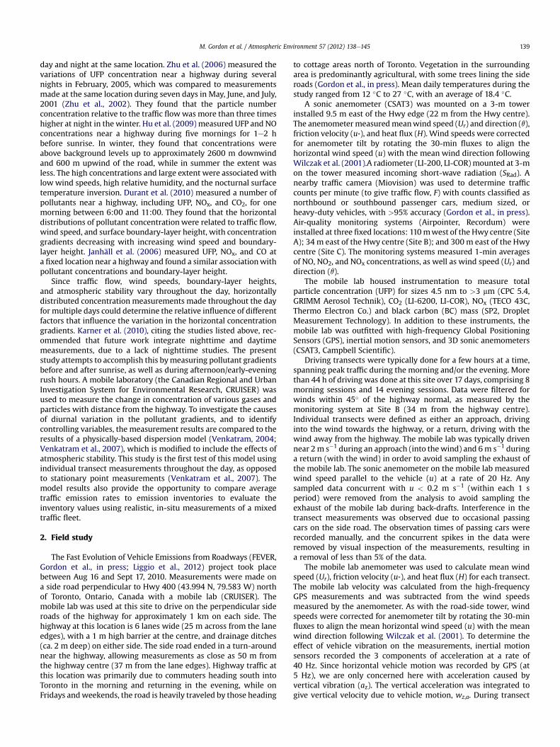
kgw0T 0

whereu* is the frictionvelocity, T is the temperature inKelvin, k¼0.4is the von Karman constant, g ¼ 9.8 m s�2 is gravitational accelera-tion, and w0T 0 is the kinematic heat flux. The three time periods arehighlighted. Peak morning traffic flow (near 110 vehicles min�1)occurred in the pre-sunrise period. In this period, the boundary-layer is relatively stable (L > 0) and friction velocity is low. Solarradiation, heat flux, instability, and friction velocity increase duringthemorning time period and traffic levels stay relatively constant atnear 90 vehicles min�1. In the evening period, solar radiation, heatflux, instability, and friction velocity decreased and traffic flowpeaked above 120 vehicles min�1. The high near-road concentra-tions before sunrise (Fig.1) are consistentwith the high traffic levelsin the pre-sunrise period (Fig. 2). Higher background levels beforesunrise are consistent with neutral stability compared to theunstable boundary-layer in the morning after sunrise and in theafternoon. This instabilitywould increase the boundary-layerheightresulting in a spread of pollutants over a greater height.

4. Dispersion model

For a conserved mass of a pollutant (i.e., without evaporation,chemical reactions, or deposition), the concentration downwind ofan infinite line source can be modeled (Venkatram, 2004) as

C ¼ Cbg þEFA

Uzcos qexp

���Bzz

�s�; (2)

where E is the emission rate per vehicle [mass per distance trav-elled], F is the vehicle flow rate [number of vehicles per unit time],U and z are the mean plume velocity and height respectively whichvary with perpendicular distance from the highway, x, s isa parameter based on stability, q is the angle between the winddirection and a line perpendicular to the highway, and z is theheight. The parameters A and B are functions of s only (givenbelow). Here we follow the derivation outlined in Venkatram(2004) for neutral conditions with the inclusion of a stabilityparameterization to account for non-neutral conditions. The meanplume height is obtained from the van Ulden (1978) formulation

440430420410400390

CO

2 [ppm]

800600400200

Distance from road, x [m]

2500020000150001000050000

UFP [cm

-3]

2.5

2.0

1.5

1.0

0.5

0.0

BC

[µg m-3]

Pre-Sunrise (5:00 - 8:00) Morning (8:00 - 11:00) Evening (15:00 - 19:00)

ed by distance from the road for three periods.

24201612840Hour of Day [EDT]

24201612840Hour of Day [EDT]

300

200

100

0

-100

H [

W m

-2]

-500

-250

0

250

500

L [m]

160

120

80

40

0

F [

min

-1]

1000

800

600

400

200

0

SR

ad [W m

-2]

4

3

2

1

0

Ur [

m s

-1]

0.8

0.6

0.4

0.2

0.0

u* [m

s -1]

a ab bc c

Fig. 2. Median and quartile diurnal cycles of traffic flow, F (weekdays only), incoming solar radiation, SRad, heat flux, H, stability, L, average velocity, Ur (at zr ¼ 3 m), and frictionvelocity, u*. Each hourly median and quartile is derived from 31 days of data. Highlighted areas show time periods for (a) pre-sunrise, (b) morning, and (c) evening data.

M. Gordon et al. / Atmospheric Environment 57 (2012) 138e145 141

dzdx

¼ KðqzÞUðqzÞ qz (3)

where K is the eddy diffusivity for mass, U is the wind speed, and qis a function of s only (given below). Following Garratt (1994), theeddy diffusivity is defined as

K ¼ ku*z=FW (4)

where FW is a stability function for water vapour diffusivity (usedto represent all scalar diffusivities), approximated by

FW ¼�ð1� 16z=LÞ�1=2; z=L < 0

1þ 5z=L; z=L>0(5)

The horizontal wind speed is assumed to follow the power-lawprofile as

UðzÞ ¼ Ur

�zzr

�p

(6)

where Ur is a reference wind speed at height zr and the exponent pis determined following Huang (1979) as

p ¼ u*kUr

FM (7)

where FM is a stability function for momentum diffusivityapproximated by (Garratt, 1994),

FM ¼�ð1� 16zr=LÞ�1=4; zr=L < 0

1þ 5zr=L; zr=L>0: (8)

Combining Eqs. (3), (4), and (6) gives

Zz

0

z0pFW

�z0.L�dz0 ¼ ku*z

pr

Urqpx (9)

which can be solved numerically to give z as a function of x.Following Venkatram (2004), a release height, h0, can be approxi-mated by introducing a virtual distance x0 at which z ¼ h0. Thevirtual distance is determined by interpolation between the valuesof xi and xiþ1 where zðxiÞ < h0 and zðxiþ1Þ > h0. The functions A, B, q,and f are given as (Venkatram, 2004)

A ¼ sBGð1=sÞ;B ¼ Gð2=sÞ

Gð1=sÞ;q ¼ ðsBsÞ1=ð1�sÞ; f ¼ Gððpþ1Þ=sÞ

Gð1=sÞBp ; (10)

where G(r) is the gamma function given byZ N

0xr�1expð�xÞdx.

An analytical solution is possible if it is assumed that thestability function can be approximated from the reference height,such that FW

�z.L�

¼ FW

�zr.L�. This gives

z ¼�ðpþ 1Þku*zprFWUrqpcosq

x�1=ðpþ1Þ

: (11)

For the analytical approximation, the denominator of Eq. (2) canbe expressed in terms of the release height as

U zcosq ¼ ðpþ 1Þu*f kFWqp

xþ fUrhpþ10 cosq

zpr: (12)

5. Model results

Median stability, L, friction velocity, u*, reference wind speed, Ur,(all at zr¼ 3.0m) and traffic flow, F, were calculated from themobilelab anemometer and road-side traffic towermeasurements for eachtransect. These values were used to determine the parameters ofEqs. (3)e(10) with a value of s ¼ 2 (Venkatram, 2004) and a releaseheight of h0 ¼ 0.5 m. The mean plume height, z, was calculatednumerically with a resolution of 0.1 m in x and 0.01 m in z. A least-squares fit of Eq. (2) was calculated for each transect, minimizingthe root-mean square error of the 1 Hz data as a function of Cbg andE, with the constraint of Cbg � 0. The resulting emission rates (E)

Table 1The emission rate quartiles (E25%, E50%, E75%) determined from least-squares fits of Eq. (2) to n transects is compared to the range of emission rates from MGEM (CO2) and themobile 6.2 model (all others). The units of E are [g km�1] with the exception of UFP [109 particles km�1]. See text for details of the inventory emissions calculations. The averagecorrelation coefficient (r2) of the least-squares fits are shown. NOx (A, B, C) gives the emission rate and r2 determined by Eq. (2) fit to the 30-min stationary measurements atsites A, B, and C simultaneous with the mobile-lab measurements.

Pollutant This study Inventory

E25% E50% E75% n r2 EM,Min EM,Max

CO2 105.2 203.2 415.6 209 0.50 228 248BC 2.0 � 10�3 5.2 � 10�3 12.7 � 10�3 181 0.45 0.88 � 10�3 2.6 � 10�3

NOx 0.20 0.39 0.99 209 0.67 0.35 0.49NO 0.05 0.11 0.25 209 0.62 N/ANO2 0.11 0.23 0.68 209 0.50 N/AUFP 14.5 37.4 146.5 192 0.53 N/ANOx (A, B, C) 0.29 0.37 0.48 76 0.97 0.35 0.49

M. Gordon et al. / Atmospheric Environment 57 (2012) 138e145142

and fit correlations (r2) are listed in Table 1 for a number ofmeasured pollutants. The interquartile ranges of the emission ratesare presented to demonstrate the range of modeled values. Usingthe analytical approximation of Eqs. (11) and (12) in lieu of thenumerical model resulted in changes in the median emission ratesof less than 10%. However, the following analysis presents resultsfrom the numerical model (Eqs. (3)e(10)) only.

The average correlation coefficients demonstrate a reasonableagreement between the model and measured data(0.45 < r2 < 0.67). Fig. 3 is a 2-dimensional histogram of the 1 Hzmeasured and modeled NOx concentrations. Although there aremany outliers, more than half of the modeled concentrations arewithin 20% of the measured concentrations. As concluded byVenkatram (2004), the model is not sensitive to the choice of s.Here, the average emission rates calculated with s ¼ 1.5 or s ¼ 3were all within 9% of the average emission rates calculated withs ¼ 2. There is also no significant change in the values of r2 usingdifferent values of s.

As some heavy-duty vehicles have exhaust heights near 4 m,the estimated release height of h0 ¼ 0.5 m may be a source oferror. Using a release height of h0 ¼ 0 m results in medianemission rates between 1% and 4% lower than emission ratesusing h0 ¼ 0.5 m. Increasing the release height to 2 m results inmedian emission rates between 9% and 17% higher, whileincreasing the release height to 4 m results in median emissionrates as much as 60% higher. Compared to h0 ¼ 0.5 m, changes inthe values of r2 for different heights (h0 ¼ 0, 2, and 4 m) arenegligible (<2%). Hence we estimate h0 ¼ 0.5 m and note thatemission rates may be higher due to an underestimated releaseheight, especially for pollutants released primarily from heavy-duty vehicles, such as BC.

Fig. 3. 2-D Histogram of measured and modeled 1 Hz concentrations from the mobile-lab transect measurements. Each bin is 0.5 mg m�3 by 0.5 mg m�3. Solid lines show 2:1,1:1, and 1:2 ratios.

As discussed in Section 3.1, pollutants such as NO, NO2, and UFPare not conserved during mixing downwind of the highway due tonear-source chemical reactions, coagulation, and evaporationprocesses. This is supported by the concentration-distance profilesshown in Fig. 1. Although the dispersion model assumes inertspecies, the average correlation coefficients (Table 1) are lowest forBC and CO2, which are both conserved during mixing. Thissuggests that, although the effects of chemical reactions, coagu-lation, and evaporation are seen in the average gradients, theseeffects do not appear to influence the relative performance of thedispersion model. This may be due to variability in measurementsof different pollutants being greater than the error in the modeldue to not modeling chemical reactions, coagulation, andevaporation.

The model was also used with the measurements of NOx at thethree stationary sites (A, B, and C). For this approach, measure-ments of NOx concentration, stability, friction velocity, referencewind speed (all at zr ¼ 3.0 m) and traffic flow were averaged in 30-min intervals. Stability, L, friction velocity, u*, reference wind speed,Ur, were determined from the road-side tower anemometer. Least-squares fits of Eq. (2) were calculated for each 30-min interval usingthe NOx concentration values at the upwind location (Site A, withEq. (2) reduced to C¼ Cbg), near downwind (Site B, x¼ 34m) and fardownwind (Site C, x ¼ 300 m). As with the fitting of the transectmeasurements, the root-mean square error was minimized asa function of Cbg and E. Data were filtered for time periods withwind directions within 45� of perpendicular to the highway (fromthe west) to ensure that Site A was upwind and Sites B and C weredownwind of the highway. This resulted in 422 30-min periodsthroughout the study. To compare similar time periods, onlyperiods which were simultaneous with the mobile-lab measure-ments were used, resulting in 76 intervals.

The resulting emission rates and average fit statistics are listedin Table 1. Although only 76 30-min intervals were used, thestatistics demonstrate a good fit of measured and model data, witha high r2 value compared to themobile measurements. These betterstatistics are likely due to the longer averaging time of themeasurements (30min versus 1 Hz) and the fitting of Eq. (2) to only3 spatial points per 30-min period. The measured and modeled 30-min NOx concentrations are compared in Fig. 4. The modeledconcentrations are very close to the measured concentrations atSite B (34m downwind), while the model tends to overestimate thebackground concentrations (Site A) and underestimate the fardownwind concentrations (Site C). Increasing the input wind speeddecreases the overestimation at Site A and the underestimation atSite C, while decreasing the input wind speed has the oppositeeffect. Since an increase in horizontal advection improves theresults, this suggests that the modeled advection of pollutants maybe too slow or the modeled mixing of the pollutants may be toorapid.

3.0

2.5

2.0

1.5

1.0

0.5

0.0

EN

Ox

[g k

m-1

]

24201612840

Fraction HDDV [%]

Model HDDV8A HDDV2B

Fig. 5. The median hourly NOx emission rates (from the stationary measurements)compared to the average hourly truck (HDDV) fraction. Error bars show quartile ranges.The emission rates calculated with the lowest and highest inventory HDDV emissionrates are shown.

150

100

50

0

Mod

eled

CN

Ox

[µg

m-3

]

150100500

Measured CNOx [µg m-3

]

A (upwind)

B (34 m)

C (300 m)

Fig. 4. Scatter plot of measured and modeled concentrations from the 3 stationaryroad-side sites. Each measurement is a 30-min average. Solid lines show 2:1, 1:1, and1:2 ratios.

M. Gordon et al. / Atmospheric Environment 57 (2012) 138e145 143

The generally good agreement between the model andmeasured data using both stationary and mobile measurementsdemonstrates the ability of the model to accurately simulate indi-vidual gradients using measured values of traffic flow, wind speed,stability, and friction velocity. Based on these results, two investi-gations are outlined in the following sections. Firstly, the modeledemission rates are compared with inventory emission rates.Secondly, diurnal measurements of traffic flow, wind speed,stability, and friction velocity are used to study the diurnal variationof the gradients, and to identify the controlling variables that resultin the diurnal variation.

6. Comparison to inventory emission rates

The modeled emission rates can be compared to inventoryvalues, derived here from the Mobile 6.2 model (http://www.epa.gov/oms/m6.htm) modified to represent the Ontario fleet averagefor 28 individual vehicle classes. Mobile 6.2C BC emission factorswere generated using SPECIATE 4.2 (http://www.epa.gov/ttn/chief/software/speciate/index.html) by splitting PM2.5 mass emissionsinto BC and OC (Profile 92050, 19% BC bymass). CO2 emissions weregenerated from a Mobile Greenhouse gas Emissions Model(MGEM). See Liggio et al. (2012) for further details. The averagefraction of heavy-duty vehicles during transects was measured tobe approximately 4%. Hence, the average mixed fleet vehicleemission rate is calculated as

EM ¼ fLEL þ fHEH (13)

where fL ¼ 0.96 and fH ¼ 0.04 are the fraction of light-duty gasoline(LDG) and heavy-duty diesel (HDD) vehicles, respectively, and ELand EH are the emission rates of light-duty gasoline and HDDvehicles, respectively. Although some light-duty vehicles countedby the traffic camera may be diesel, this is a small fraction of thefleet (ca. 1.3%, NRC, 2009) and the effect is assumed to be negli-gible. For HDD vehicles, there are 8 classes of vehicles in theinventory, which are dependent on vehicle weight. Since thedistribution of HDD vehicle weights is unknown, we use a limitingrange of values based on the minimum and maximum HDDemission rates.

The calculated inventory emission rates are compared to themodeled emission rates in Table 1. The median modeled CO2emission rate is 10% less than the minimum inventory value and18% less than the maximum inventory value. Given the large vari-ation in the modeled emission rate (as demonstrated by the quar-tile values) this is a relatively good agreement. The median

modeled black carbon emission rate is significantly higher than theMobile 6.2 emission rates by a factor between 2.0 and 5.9,depending on the HDD emission rate used. This is consistent withthe results of Liggio et al. (2012), which suggest that the inventoryemission rate of LDG vehicles is underestimated by a factor of 8e9.Increasing the inventory LDGV emission rate by a factor of 8.5results inminimum andmaximum inventory fleet emission rates of4.7 and 6.4 mg km�1, respectively. This range is consistent with themedian modeled black carbon emission rate of 5.2 mg km�1. Themedian modeled NOx emission rate (0.39 g km�1) is between theminimum and maximum inventory values, demonstrating verygood agreement. The modeled NOx emission rate determined usingthe stationary measurements (0.37 g km�1) is very close to themodeled NOx emission rate using the mobile measurements.Although this agreement is likely fortuitous given the uncertaintiesinvolved, it is a supportive assessment of the model’s predictiveability.

Although the modeled emission rate determined usingstationary measurements and listed in Table 1 was for time-periods concurrent with the mobile-lab measurements, the auto-mated stationary measurements were made continuously day andnight. This allowed for a grouping of modeled emission rates byhour of day, which is compared to the hourly fraction of heavy-duty vehicles in Fig. 5. As above, all measurements are filteredfor wind speeds within 45� of perpendicular to the highway (fromthe west) resulting in 422 30-min intervals. The median hourlyemission rates demonstrate a clear increase with heavy-dutyvehicle fraction, which is compared to Eq. (13) using both theminimum and maximum HDDV inventory emission rates (EH).Since the HDD fleet is likely a mix a various HDD types, theexpected emission rate should be somewhere between themaximum and minimum values of Eq. (13). However, for highfractions of heavy-duty traffic, most of the modeled emission ratesare close to the inventory values determined using the highestemission HDDV. Although there is a large amount of variation inthe modeled emission rates at high HDDV fractions, the correlationwith the median values is very good (r2 ¼ 0.93). As discussed inSection 6, using a higher release height (h0) would increase themodeled emission rate and further increase the differencebetween measured and modeled emission rates at high HDDVfractions. Hence, these results suggests that the inventory valuescould underestimate the emissions of the HDDV fleet at thislocation.

120

80

40

0

C [

µg m

-3]

242220181614121086420

Hour of Day [EDT]

100

90

80

70

x 1/2

[m

]

Measured, CB – CA

Modeled, C(36m)

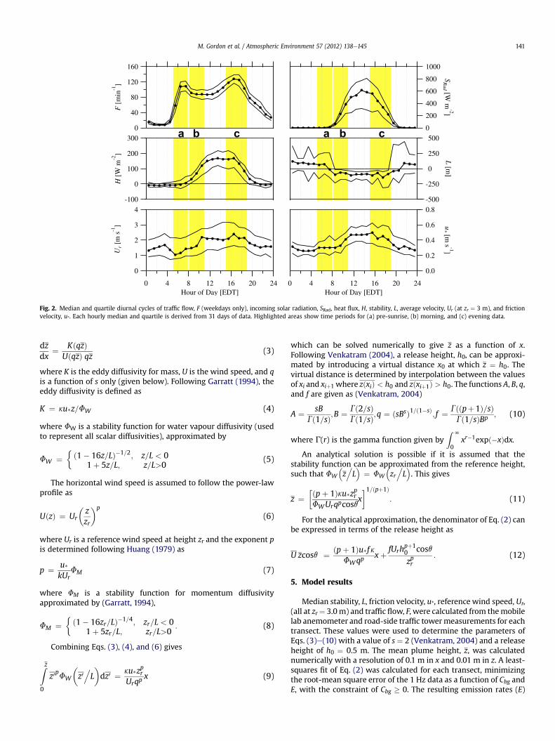
Fig. 7. Diurnal variation of the modeled and measured NOx concentration at x ¼ 36 m.The background at upwind Site A (CA) is subtracted from the measured concentrationat Site B (CB). Error bars show upper and lower quartiles of the measurements. Themodeled half-distance (x1/2) is the distance at which C(x1/2) ¼ ½ C(36 m), where C isthe modeled NOx concentration.

M. Gordon et al. / Atmospheric Environment 57 (2012) 138e145144

7. Modeled diurnal variation

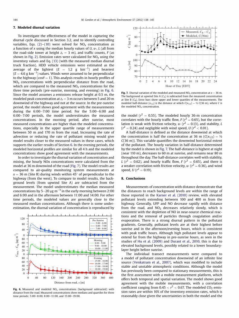
To investigate the effectiveness of the model in capturing thediurnal cycle discussed in Section 3.2, and to identify controllingvariables, Eqs. (2)e(10) were solved for NOx concentration asa function of x using the median hourly values of U, u*, L (all fromthe road-side tower at height zr ¼ 3 m), and traffic counts, F (asshown in Fig. 2). Emission rates were calculated for NOx using theinventory values and Eq. (13) (with the measured median diurnaltruck fraction). HDD vehicle emissions were estimated as theaverage of the lightest (E ¼ 1.2 g km�1) and heaviest(E ¼ 4.6 g km�1) values. Winds were assumed to be perpendicularto the highway (cosq ¼ 1). This analysis results in hourly profiles ofNOx concentrations with perpendicular distance from the road,which are compared to the measured NOx concentrations for thethree time periods (pre-sunrise, morning, and evening) in Fig. 6.Since the model assumes a emissions release height at 0.5 m, themodeled peak concentration at zr¼ 3m occurs between 5 and 20mdownwind of the highway and not at the source. In the pre-sunriseperiod, the model shows good agreement with the measurementsduring the 6:00e7:00 time period. For the 5:00e6:00 and6:00e7:00 periods, the model underestimates the measuredconcentrations. In the morning period, after sunrise, mostmeasured concentrations are higher than the modeled concentra-tions, especially in the upper quartile range of measurementsbetween 50 m and 170 m from the road. Increasing the rate ofadvection or reducing the rate of pollutant mixing would givemodel results closer to the measured values in these cases, whichsupports the earlier results of Section 6. In the evening periods, themodeled horizontal profiles are similar for all 4 h and the modeledconcentrations show good agreement with the measurements.

In order to investigate the diurnal variation of concentration andmixing, the hourly NOx concentrations were calculated from themodel at 36 m downwind of the road (Fig. 7). The model results arecompared to air-quality monitoring system measurements atx ¼ 36 m (Site B) during winds within 45� of perpendicular to thehighway (from the west). To compare to model results, the back-ground levels (from upwind Site A) are subtracted from themeasurement. The model underestimates the median measuredconcentrations by 5e20 mg m�3 in the early morning between 2:00and 6:00 and in the afternoon between 11:00 and 14:00. For othertime periods, the modeled values are generally close to themeasured median concentrations. Although there is some under-estimation, the diurnal variation of concentration is reproduced by

120

80

40

080604020

0CN

Ox

– C

bg [

µg m

-3]

80604020

0

40036032028024020016012080400

Distance from road, x [m]

Pre-Sunrise 5:00 - 6:00 6:00 - 7:00 7:00 - 8:00

Morning 8:00 - 9:00 9:00 - 10:00 10:00 - 11:00

Evening 15:00 - 16:00 16:00 - 17:00 17:00 - 18:00 18:00 - 19:00

Fig. 6. Measured and modeled NOx concentrations (background subtracted) withdistance from the road. Measured concentrations showmedians and quartiles for threetime periods: 5:00e8:00, 8:00e11:00, and 15:00e19:00.

the model (r2 ¼ 0.55). The modeled hourly 36-m concentrationcorrelates with the hourly traffic flow, F (r2 ¼ 0.65), but the corre-lation is weak with friction velocity, u* (r2 ¼ 0.13), and stability, L(r2 ¼ 0.24) and negligible with wind speed, U (r2 < 0.01).

A half-distance is defined as the distance downwind at whichthe concentration is half the concentration at 36 m (C(x1/2) ¼ ½C(36 m)). This variable quantifies the downwind horizontal extentof the pollutant. The hourly variation in half-distance determinedby the model is shown in Fig. 7. The half-distance is highest at night(near 110 m), decreases to 60 m at sunrise, and remains near 80 mthroughout the day. The half-distance correlates well with stability,L (r2 ¼ 0.62), and hourly traffic flow, F (r2 ¼ 0.65), and there isa weaker correlation with friction velocity, u* (r2 ¼ 0.36), and windspeed, U (r2 ¼ 0.19).

8. Conclusions

Measurements of concentrationwith distance demonstrate thatthe distances to reach background levels are within the range ofthose reported in the Karner et al. (2010) review, with elevatedpollutant levels extending between 100 and 400 m from thehighway. Generally, UFP and NO decrease rapidly with distancefrom the road, and NO2 decreases relatively slowly, which isconsistent with the depletion of NO in near-source chemical reac-tions and the removal of particles through coagulation and/orevaporation. There is a strong diurnal pattern in the pollutantgradients. Generally, pollutant levels are at their highest beforesunrise and in the afternoon/evening hours, which is consistentwith peak traffic hours. Although high pollutant levels appear toextend far from the highway in pre-sunrise hours, as seen in thestudies of Hu et al. (2009) and Durant et al., 2010, this is due toelevated background levels, possibly related to a lower boundary-layer height before sunrise.

The individual transect measurements were compared toa model of pollutant concentration downwind of an infinite linesource (Venkatram et al., 2007), which was modified to includestable and unstable atmospheric conditions. Although the modelhas previously been compared to stationary measurements, this isthe first assessment with a mobile measurement platform, whichoffers both temporal and spatial variation. The model shows goodagreement with the mobile measurements, with a correlationcoefficient ranging from 0.45 < r2 < 0.67. The modeled CO2 emis-sion rates are within 10% of the inventory emission rates, which isreasonably close given the uncertainties in both the model and the

M. Gordon et al. / Atmospheric Environment 57 (2012) 138e145 145

inventory values. The modeled NOx emission rates are very close toaverage inventory values. Model BC emission rates are betweena factor of 2.0 and 5.9 higher than inventory values, which supportsthe conclusion that BC emissions from gasoline are under-estimated, as seen in the results of Liggio et al. (2012). Medianhourly NOx emission rates modeled with 24-h stationarymeasurements demonstrate a strong correlation (r2 ¼ 0.93) withthe hourly fraction of heavy-duty vehicles. For high heavy-dutyvehicle fractions, the modeled emission rates are generally closeto the inventory values of emission rates for the worst HDDV,suggesting that the inventory emission rates may underestimatethe true fleet-average HDDV emission rates. If true, this suggeststhat retrofitting HDDV could have a substantial impact on totalemissions. However, these results are supported by only 3 h duringwhich high fractions (>10%) of HDDV are seen.

By usingmeasured hourly wind, turbulence, and traffic values asinput, the model is able to capture the same diurnal cycles seen inthe measured pollutant gradients, although there are quantitativedifferences. The modeled near-road concentrations and the half-distance both demonstrate a strong correlation with traffic flow.The half-distance also shows a correlationwith friction velocity andstability. These results demonstrate the applicability of this rela-tively easy to use model, which offers many advantages includingaccurate estimations of average traffic emission rates, as well asmodel results at different heights, and the determination of thevertical extent of the highway plume.

Acknowledgements

This work was supported by the Natural Science and Engi-neering Research Council of Canada and was funded by the Scienceand Technology Branch, Environment Canada and the Particles andRelated Emission Project (PERD) C11.008, which is a programadministered by Natural Resources Canada.

References

Brook, R.D., Brook, J.R., Urch, B., Vincent, R., Rajagopalan, S., Silverman, F., 2002.Inhalation of fine particulate air pollution and ozone causes acute arterialvasoconstriction in healthy adults. Circulation 105, 1534e1536.

Brugge, D., Durant, J.L., Rioux, C., 2007. Near-highway pollutants in motor vehicleexhaust: a review of epidemiologic evidence of cardiac and pulmonary healthrisks. Environ. Health 6, 23.

Brunekreef, B., Janssen, N.A.H., deHartog, J., Harssema, H., Knape, M., van Vliet, P.,1997. Air pollution from truck traffic and lung function in children living nearmotorways. Epidemiology 8, 298e303.

Durant, J.L., Ash, C.A., Wood, E.C., Herndon, S.C., Jayne, J.T., Knighton, W.B.,Canagaratna, M.R., Trull, J.B., Brugge, D., Zamore, W., Kolb, C.E., 2010. Short-Termvariation in near-highway air pollutant gradients on a winter morning. Atmos.Chem. Phys. Discuss. 2010 (10), 5599e5626.

Garratt, J.R., 1994. The Atmospheric Boundary Layer. Cambridge University Press,Cambridge.

Gordon, M., Staebler, R.M., Liggio, J., Makar, P., Brook, J., Li, S.-M., Wentzell, J., Lu, G.,Lee, P., Measurements of enhanced turbulent mixing near highways. Appl.Meteorol. in press.

Health Effects Institute, 2010. Traffic-Related Air Pollution. Special Report 17. BostonMassachusetts.

Hoek, G., Brunekreef, B., Goldbohm, S., Fischer, P., van den Brandt, P.A., 2002.Association between mortality and indicators of traffic-related air pollution inthe Netherlands: a cohort study. The Lancet 360, 203e1209.

Hu, S., Fruin, S., Kozawa, K., Mara, S., Paulson, S.E., Winer, A.M., 2009. A wide area ofair pollutant impact downwind of a freeway during pre-sunrise hours. Atmos.Environ. 43, 2541e2549.

Huang, C.H., 1979. A theory of dispersion in turbulent shear flow. Atmos. Environ.13, 453e463.

Janhäll, S., Olofson, K.F.G., Andersson, P.U., Pettersson, J.B.C., Hallquist, M., 2006.Evolution of the urban aerosol during winter temperature inversion episodes.Atmos. Environ. 40, 5355e5366.

Karner, A.A., Eisinger, D.S., Niemeier, D.A., 2010. Near-roadway air quality:synthesizing the findings from real-world data. Environ. Sci. Technol. 44,5334e5344.

Kuhn, T., Biswas, S., Sioutas, C., 2005. Diurnal and seasonal characteristics of particlevolatility and chemical composition in the vicinity of a light-duty vehiclefreeway. Atmos. Environ. 39, 7154e7166.

Liggio, J., Gordon, M., Brook, J., Smallwood, G., Li, S.-M., Stroud, C., Staebler, R.M.,Lu, G., Lee, P., Taylor, B., 2012. Are emissions of black carbon from gasolinevehicles underestimated? Insights from near and on-road measurements.Environ. Sci. Technol. 46 (9), 4819e4824.

Lin, S., Munsie, J.P., Hwang, S.-A., Fitzgerald, E., Cayo, M.R., 2002. Childhood asthmahospitalization and residential exposure to state route traffic. Environ. Res. 88,71e81.

Natural Resources Canada, Office of Energy Efficiency, 2009. Canadian VehicleSurvey: Summary Report, ISBN 978-0-662-06802-0.

Pearson, R.L., Watchel, H., Ebi, K.L., 2000. Distance-weighted traffic density inproximity to a home is a risk factor for leukemia and other childhood cancers.J. Air Waste Manage. Assoc. 50, 175e180.

U.S. Census Bureau, 2008. Current Housing Reports, Series H150/07. In: AmericanHousing Survey for the United States: 2007. U.S. Government Printing Office,Washington, DC, 20401.

van Ulden, A.P., 1978. Simple estimates for vertical dispersion from sources near theground. Atmos. Environ. 12, 2125e2129.

van Vliet, P., Knape, M., de Hartog, J., Janssen, N., Harssema, H., Brunekreef, B., 1997.Motor vehicle exhaust and chronic respiratory symptoms in children living nearfreeways. Environ. Res. 74 (2), 122e132.

Venkatram, A., 2004. On estimating emission through horizontal fluxes. Atmos.Environ. 38, 1337e1344.

Venkatram, A., Isakov, V., Thoma, E., Baldauf, R., 2007. Analysis of air quality datanear roadways using a dispersion model. Atmos. Environ. 41, 9481e9497.

Venn, A.J., Lewis, S.A., Cooper, M., Hubbard, R., Britton, J., 2001. Living near a mainroad and the risk of wheezing illness in children. Am. J. Respir. Care Med. 164,2177e2180.

Wilczak, J.M., Oncley, S.P., Stage, S.A., 2001. Sonic anemometer tilt correctionalgorithms. Bound.-Lay. Meteorol. 99, 127e150.

Zhu, Y., Hinds, W., Kim, S., Sioutas, C., 2002. Concentration and size distribution ofultrafine particles near a major highway. J. Air Waste Manag. Assoc. 52,1032e1042.

Zhu, Y., Kuhn, T., Mayo, P., Hinds, W.C., 2006. Comparison of daytime and nighttimeconcentration profiles and size distributions of ultrafine particles near a majorhighway. Environ. Sci. Technol. 40, 2531e2536.

Zhou, Y., Levy, J., 2007. Factors influencing the spatial extent of mobile source airpollution impacts: a meta-analysis. BMC Public Health 7 (1), 89.