ME-406 EXERCISE #18 SPRING, 1999 - University of ...jbaker/ansys-fluids1.doc · Web viewDefine...
36
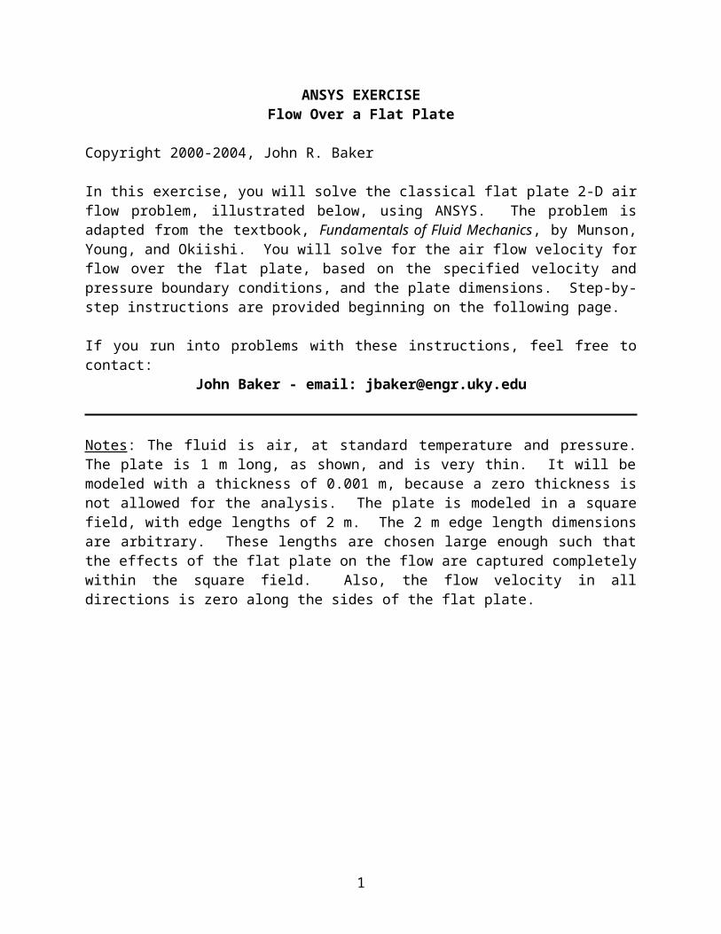
ANSYS EXERCISE Flow Over a Flat Plate Copyright 2000-2004, John R. Baker In this exercise, you will solve the classical flat plate 2-D air flow problem, illustrated below, using ANSYS. The problem is adapted from the textbook, Fundamentals of Fluid Mechanics, by Munson, Young, and Okiishi. You will solve for the air flow velocity for flow over the flat plate, based on the specified velocity and pressure boundary conditions, and the plate dimensions. Step-by- step instructions are provided beginning on the following page. If you run into problems with these instructions, feel free to contact: John Baker - email: [email protected] Notes : The fluid is air, at standard temperature and pressure. The plate is 1 m long, as shown, and is very thin. It will be modeled with a thickness of 0.001 m, because a zero thickness is not allowed for the analysis. The plate is modeled in a square field, with edge lengths of 2 m. The 2 m edge length dimensions are arbitrary. These lengths are chosen large enough such that the effects of the flat plate on the flow are captured completely within the square field. Also, the flow velocity in all directions is zero along the sides of the flat plate. 1
Transcript of ME-406 EXERCISE #18 SPRING, 1999 - University of ...jbaker/ansys-fluids1.doc · Web viewDefine...
ANSYS EXERCISEFlow Over a Flat Plate
Copyright 2000-2004, John R. Baker
In this exercise, you will solve the classical flat plate 2-D air flow problem, illustrated below, using ANSYS. The problem is adapted from the textbook, Fundamentals of Fluid Mechanics, by Munson, Young, and Okiishi. You will solve for the air flow velocity for flow over the flat plate, based on the specified velocity and pressure boundary conditions, and the plate dimensions. Step-by-step instructions are provided beginning on the following page.
If you run into problems with these instructions, feel free to contact: John Baker - email: [email protected]
Notes: The fluid is air, at standard temperature and pressure. The plate is 1 m long, as shown, and is very thin. It will be modeled with a thickness of 0.001 m, because a zero thickness is not allowed for the analysis. The plate is modeled in a square field, with edge lengths of 2 m. The 2 m edge length dimensions are arbitrary. These lengths are chosen large enough such that the effects of the flat plate on the flow are captured completely within the square field. Also, the flow velocity in all directions is zero along the sides of the flat plate.
1
1 m
2 m
2 m
Veloc
ity=0
.0727
64 m
/s
AtmosphericPressure
AtmosphericPressure

The steps that will be followed, after launching ANSYS, are:
Preprocessing:1. Change Jobname.2. Define element type. (Fluid141 element, which is a 2-D element for fluid analysis.)3. Define the fluid. (Air – SI Units.)4. Create keypoints.5. Create areas.6. Specify meshing controls / Mesh the areas to create nodes and elements. 7. Zoom in to see flat plate region (optional).
Solution:8. Specify boundary conditions. 9. Specify number of solution iterations.10. Solve.
Postprocessing:11. Plot the x-direction velocity (VX) distribution.12. List VX at Nodes.
Exit13. Exit the ANSYS program, saving all data._____________________________________________________________________________
Launching ANSYS:
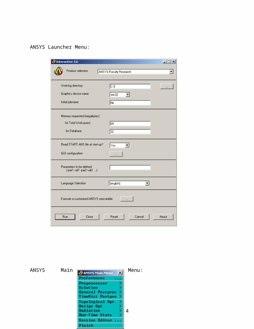
It is probably best to save your work on a Zip Disk in the computer IOMEGA Zip Drive. On any machine in the computer lab (on the first floor of Crounse Hall), insert a Zip Disk in the drive. Then, simply click on the ANSYS icon on the Windows Desktop. The ANSYS Launcher menu should appear. It is shown at the top of the next page. The only input you will likely need on this menu is specification of the Zip Drive as your “Working Directory”. If you don’t have a Zip Disk, or if you prefer to work on the computer hard drive instead, then specify any directory (or, “Folder”) as your working directory. To browse and find the desired working directory, click on the button with the three dots to the far right on the Launcher Menu on the line that says “Working Directory”. Once the working directory is specified, click on “Run” at the bottom of the Launcher Menu.
The ANSYS menus should open up. You will see a Main Menu, illustrated on the following page, and a large black graphics window. You are now ready to begin creating the model and performing the analysis.
2

ANSYS Launcher Menu:
ANSYS Main Menu:
3
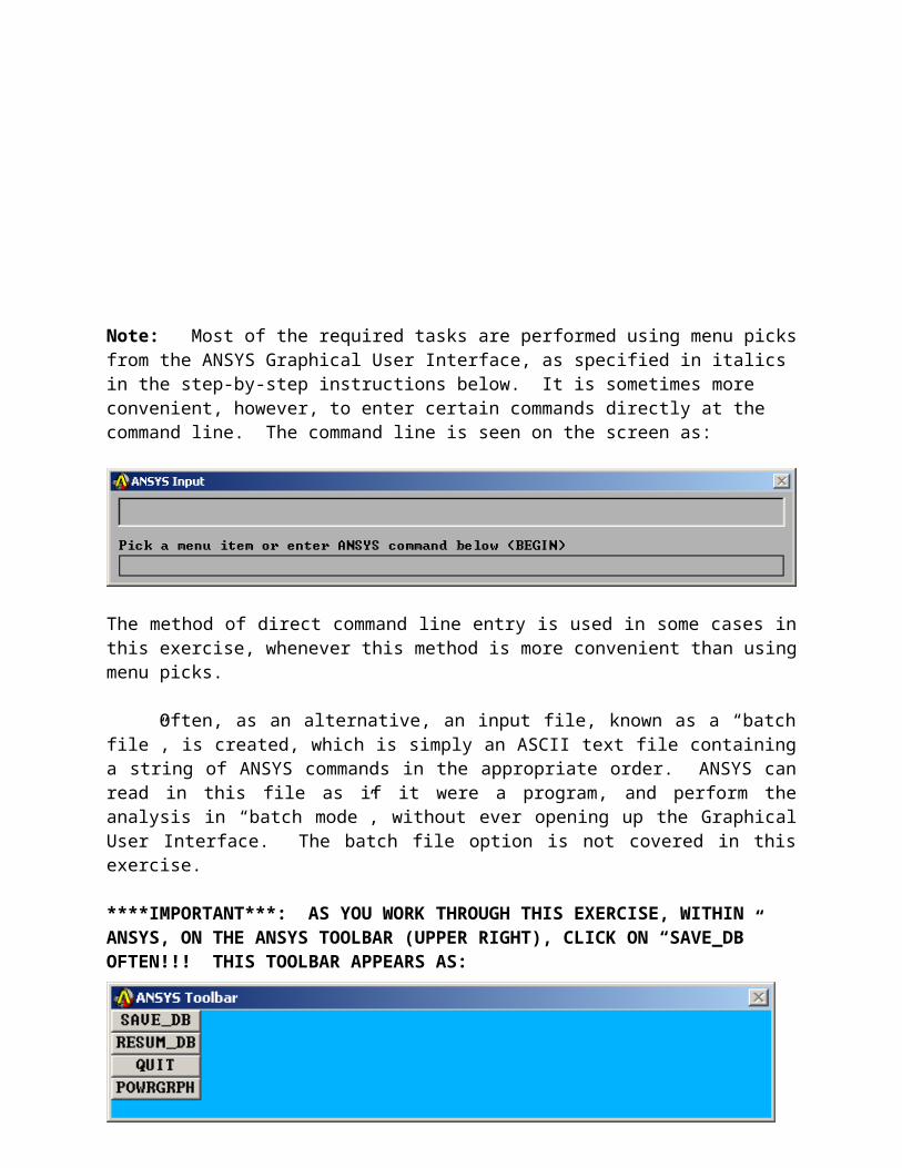
Note: Most of the required tasks are performed using menu picks from the ANSYS Graphical User Interface, as specified in italics in the step-by-step instructions below. It is sometimes more convenient, however, to enter certain commands directly at the command line. The command line is seen on the screen as:
The method of direct command line entry is used in some cases in this exercise, whenever this method is more convenient than using menu picks.
Often, as an alternative, an input file, known as a “batch file”, is created, which is simply an ASCII text file containing a string of ANSYS commands in the appropriate order. ANSYS can read in this file as if it were a program, and perform the analysis in “batch mode”, without ever opening up the Graphical User Interface. The batch file option is not covered in this exercise.
****IMPORTANT***: AS YOU WORK THROUGH THIS EXERCISE, WITHIN ANSYS, ON THE ANSYS TOOLBAR (UPPER RIGHT), CLICK ON “SAVE_DB” OFTEN!!! THIS TOOLBAR APPEARS AS:
At any point, if you want to resume from the previous time the model was saved, simply click on “RESUM_DB” on this same Toolbar. Any information entered since the last save will be lost, but this is a nice feature in the event that you make an input mistake, and are unsure of how to correct it.
There are a number of ways to model a system and perform an analysis in ANSYS. The steps below present only one method.
4
Preprocessing:
1. Change jobname. On the Utility Menu across the very top of the screen, select: File -> Change Jobname
Enter “flatplate”, and click on “OK”.
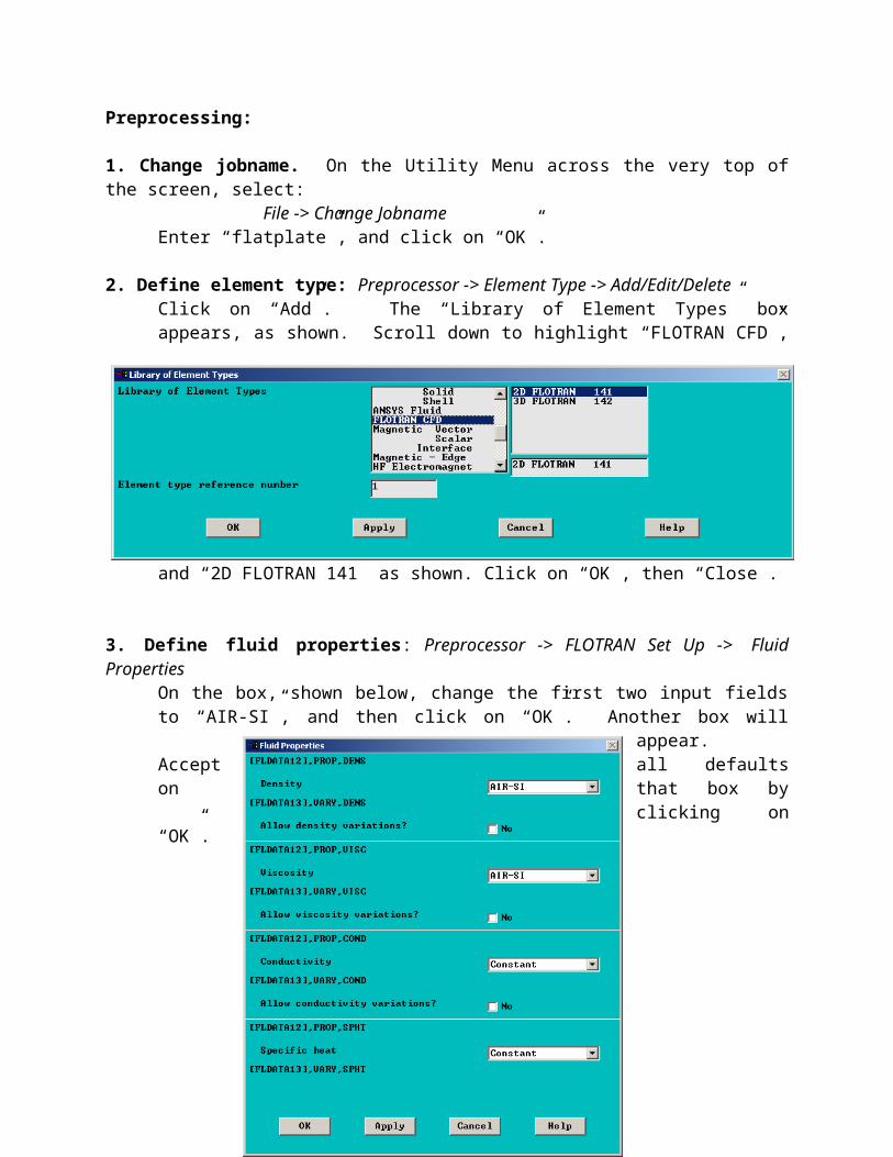
2. Define element type: Preprocessor -> Element Type -> Add/Edit/DeleteClick on “Add”. The “Library of Element Types” box appears, as shown. Scroll down to highlight “FLOTRAN CFD”, and “2D FLOTRAN 141” as shown. Click on “OK”, then “Close”.
3. Define fluid properties: Preprocessor -> FLOTRAN Set Up -> Fluid Properties On the box, shown below, change the first two input fields to “AIR-SI”, and then click on “OK”. Another box will appear. Accept all defaults on that box by clicking on “OK”.
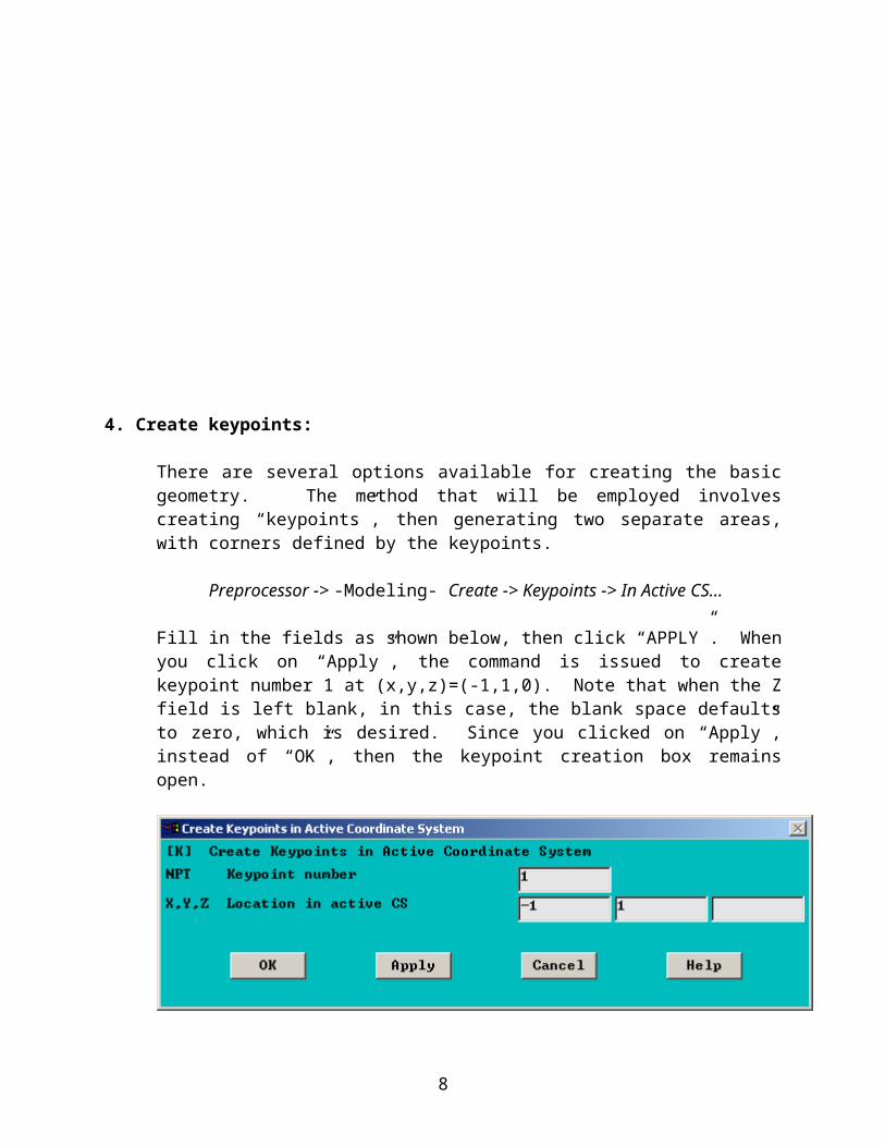
4. Create keypoints:
5
There are several options available for creating the basic geometry. The method that will be employed involves creating “keypoints”, then generating two separate areas, with corners defined by the keypoints.
Preprocessor -> -Modeling- Create -> Keypoints -> In Active CS…
Fill in the fields as shown below, then click “APPLY”. When you click on “Apply”, the command is issued to create keypoint number 1 at (x,y,z)=(-1,1,0). Note that when the Z field is left blank, in this case, the blank space defaults to zero, which is desired. Since you clicked on “Apply”, instead of “OK”, then the keypoint creation box remains open.
Create keypoint number 2 at (x,y,z)=(0,1,0), using the input shown below. After entering the input, again, click on “APPLY”:
Create 12 total keypoints in the same manner. The locations for all 12 are shown in the following table. When the final keypoint is created, click on “OK” instead of “APPLY”. “OK” issues the command and also closes the keypoint creation box.
Keypoint Number X-Location Y-Location
6
1 -1 12 0 13 1 14 -0.5 05 0 06 0.5 07 -0.5 -0.0018 0 -0.0019 0.5 -0.00110 -1 -111 0 -112 1 -1
Before moving on, it is probably a good idea to check the keypoint locations. Along the top toolbar:
Choose: List -> Keypoints -> Coordinates Only. A box should open up with the keypoint location information. If any keypoint is not in the correct location, at this point, you can just re-issue the keypoint creation command for that particular keypoint. To do this, choose: Preprocessor -> -Modeling- Create -> Keypoints -> In Active CS…
Fill in the correct information for that particular keypoint in the box, and click “OK”. The keypoint will be moved to the correct location. If you have some keypoint incorrectly numbered above number 12, this will not cause a problem. Just be sure you have keypoint numbers 1 thru 12 located correctly.
You can close the box listing the keypoint locations, by clicking, in that listing box, on “File-> Close”.
5. Create areas:
It may be a good idea to save your model at this point, by clicking “SAVE_DB” on the ANSYS Toolbar:
7
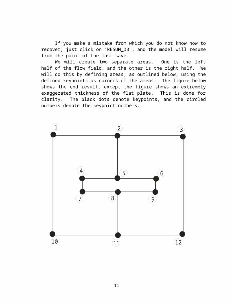
If you make a mistake from which you do not know how to recover, just click on “RESUM_DB”, and the model will resume from the point of the last save.
We will create two separate areas. One is the left half of the flow field, and the other is the right half. We will do this by defining areas, as outlined below, using the defined keypoints as corners of the areas. The figure below shows the end result, except the figure shows an extremely exaggerated thickness of the flat plate. This is done for clarity. The black dots denote keypoints, and the circled numbers denote the keypoint numbers.
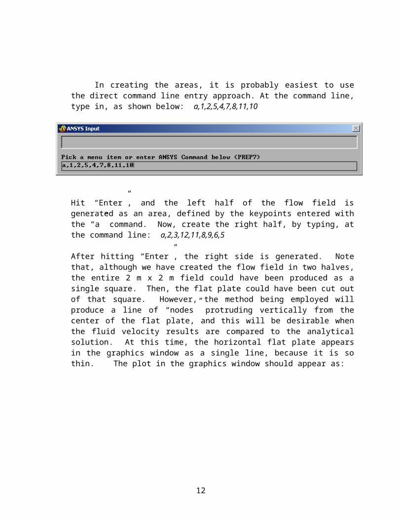
In creating the areas, it is probably easiest to use the direct command line entry approach. At the command line, type in, as shown below: a,1,2,5,4,7,8,11,10
8
1 2 3
4 5 6
7 8 9
10 11 12

Hit “Enter”, and the left half of the flow field is generated as an area, defined by the keypoints entered with the “a” command. Now, create the right half, by typing, at the command line: a,2,3,12,11,8,9,6,5
After hitting “Enter”, the right side is generated. Note that, although we have created the flow field in two halves, the entire 2 m x 2 m field could have been produced as a single square. Then, the flat plate could have been cut out of that square. However, the method being employed will produce a line of “nodes” protruding vertically from the center of the flat plate, and this will be desirable when the fluid velocity results are compared to the analytical solution. At this time, the horizontal flat plate appears in the graphics window as a single line, because it is so thin. The plot in the graphics window should appear as:
9

6. Specify Mesh Size Controls / Mesh the Model.
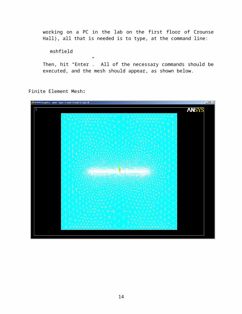
There are a number of ways to perform this step, but for this exercise, the procedure has been automated, and will involve typing only a single word, below. The actual method employed would involve entering 24 commands at the command line. Because of the possibility of typographical errors, however, for this exercise, this step has been automated, using the “macro” option within ANSYS. A macro has been created and installed on all 19 PC’s on the first floor of Crounse Hall. The commands in the macro are discussed in the Appendix, at the end of these instructions. However, to execute all of the required commands (assuming you are working on a PC in the lab on the first floor of Crounse Hall), all that is needed is to type, at the command line:
mshfield
Then, hit “Enter”. All of the necessary commands should be executed, and the mesh should appear, as shown below.
Finite Element Mesh:
10
7. Zoom in to see the flat plate (optional)
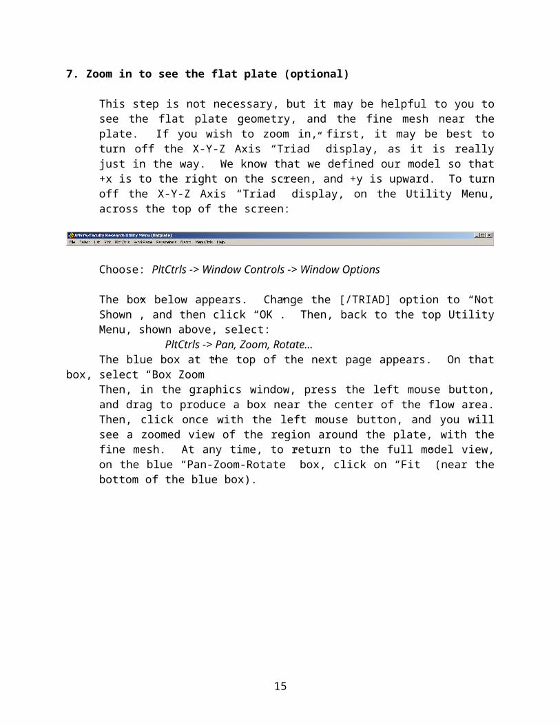
This step is not necessary, but it may be helpful to you to see the flat plate geometry, and the fine mesh near the plate. If you wish to zoom in, first, it may be best to turn off the X-Y-Z Axis “Triad” display, as it is really just in the way. We know that we defined our model so that +x is to the right on the screen, and +y is upward. To turn off the X-Y-Z Axis “Triad” display, on the Utility Menu, across the top of the screen:
Choose: PltCtrls -> Window Controls -> Window Options
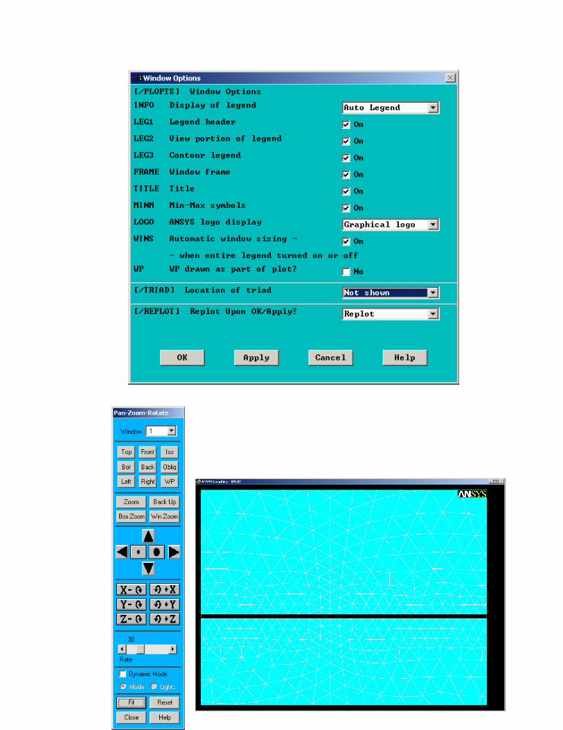
The box below appears. Change the [/TRIAD] option to “Not Shown”, and then click “OK”. Then, back to the top Utility Menu, shown above, select:
PltCtrls -> Pan, Zoom, Rotate…The blue box at the top of the next page appears. On that box, select “Box Zoom” Then, in the graphics window, press the left mouse button, and drag to produce a box near the center of the flow area. Then, click once with the left mouse button, and you will see a zoomed view of the region around the plate, with the fine mesh. At any time, to return to the full model view, on the blue “Pan-Zoom-Rotate” box, click on “Fit” (near the bottom of the blue box).
11
Solution:
8. Specify boundary conditions.
On page 8 (Step 5) there is a sketch of the geometry, with a very exaggerated thickness for the flat plate. You may want to refer to this figure and the figure on page 1, during the boundary condition specification. The boundary condition specification steps are outlined below, in steps 8a thru 8e, where VX denotes X-direction flow velocity, and VY denotes Y-direction flow velocity. Before beginning the specifications, it is probably best to plot the lines, without showing the areas, for better clarity. On the top Utility Menu:
Select: Plot -> Lines
12

You should then see colored lines, which are the boundaries of the areas. Unless you are zoomed in, the flat plate will probably appear as a single horizontal line. Although not necessary, you may also want to turn on “Keypoint Numbering”. To do this, on the top Utility Menu, choose: PltCtrls -> Numbering
The box below opens. Click on the box to the right of “Keypoint numbers” to toggle from “Off” to “On”. Then, click on “OK”. If you have the lines plotted, then the keypoint numbers should also show.
8a) Specification of VX=0.072764 and VY=0 on the line connecting keypoints 1 and 10. One way to do this is to choose:
Solution -> -Loads- Apply -> -Fluid/CFD- Velocity -> On Lines
A picking menu appears, as shown (next page, left). Click on the far left vertical line (the line which connects keypoints 1 and 10), and it should highlight. In the picking menu, choose “OK”. (Note that if you accidently highlight the wrong line, you can unselect it using the picking menu, and switching from “Pick” to “Unpick”. But here, it’s probably easiest to just hit “Cancel” on the picking menu, then re-open the picking box, using: Solution -> -Loads- Apply -> -Fluid/CFD- Velocity -> On Lines.)
13
After highlighting the appropriate line, and clicking “OK” in the Picking Menu, a box appears (shown below right). Enter “0.072764” for VX, and 0.0 for “VY”, then click “OK”. Since this is a 2-D analysis, you don’t need a VZ value.
8b) Specification of VX=VY=0.0 along the edges of the flat plate. Here, we could use the picking option to select the correct lines, as we did in Step 8a. But, it would involve zooming in to pick the correct closely-spaced lines. It may be easiest here to initially just select the correct lines, using two successive command line entries, which are:
14
ksel,s,kp,,4,9lslk,s,1
Hit “Enter” after each command. Note that there are supposed to be two consecutive commas, as shown, in the “ksel” command. The first command above selects keypoints 4 thru 9, and the second command selects the set of all lines which have their endpoints within the selected set of keypoints. Now, on the menus, choose:
Solution -> -Loads- Apply -> -Fluid/CFD- Velocity -> On Lines
This time, when the picking menu appears, you don’t need to pick on any lines in the model, just choose “Pick All” at the bottom of the picking menu. Only the lines of interest are currently selected. When the “Velocity Constraints” box opens, just enter VX=0.0 and VY=0.0, then click on “OK”.
Now, it is very important that you re-select all entities. On the top Utility Menu:
choose: Select -> Everything (or else, equivalently, you can type, at the command line: allsel , then hit “Enter”.
Then, all lines are probably still showing in the graphics window, but just to make sure, on the top Utility Menu, choose: Plot -> Lines
8c) Specification of atmospheric pressure on five of the six lines that define the outer boundary. These are the lines defined by end keypoints 1-2; 2-3; 3-12; 12-11; and 11-10. Note that the farthest left vertical line, connecting keypoints 1 and 10, is not included in the set. Here, we can return to the picking menu method. Choose:
Solution -> -Loads- Apply -> -Fluid/CFD- Pressure DOF -> On Lines
A picking menu opens. Click on all five of the lines noted above to highlight them. If you make a mistake in picking, it may be best to just click on “Cancel” in the picking menu, then re-start step 8c. Once the correct five lines are highlighted, choose “OK” in the picking menu, and the “Pressure Constraint” box will open, as shown below. Enter “0” for “Pressure value”, and click “OK”. This “0” value indicates atmospheric pressure.
15
9. Specify Number of Solution Iterations:
Solution -> FLOTRAN Set Up -> Execution Ctrl
The box below appears. Change the first input field value to 500, as shown. No other changes are needed. Click OK.
10. Solve the problem:
16

Solution -> Run FLOTRAN
You should see a plot, with “Iteration Number” along the horizontal axis. The problem will run until the specified 500 iterations are completed. This will take a few minutes. When the solution is completed, a yellow box will appear that reads “Solution is Done!”. You may close this yellow box.
Postprocessing:
11. Plot the x-direction velocity distribution.
First, read in the results by selecting:
General Postproc -> -Read Results- Last Set
Then, to plot, choose:
General Postproc -> Plot Results -> -Contour Plot- Nodal Solu
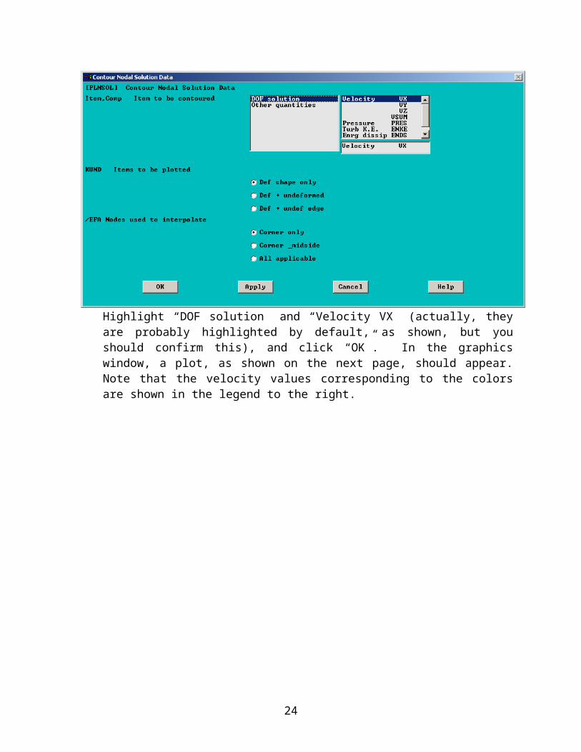
The box below opens:
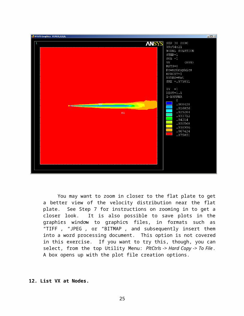
Highlight “DOF solution” and “Velocity VX” (actually, they are probably highlighted by default, as shown, but you should confirm this), and click “OK”. In the graphics window, a plot, as shown on the next page, should appear. Note that the velocity values corresponding to the colors are shown in the legend to the right.
17

You may want to zoom in closer to the flat plate to get a better view of the velocity distribution near the flat plate. See Step 7 for instructions on zooming in to get a closer look. It is also possible to save plots in the graphics window to graphics files, in formats such as “TIFF”, “JPEG”, or “BITMAP”, and subsequently insert them into a word processing document. This option is not covered in this exercise. If you want to try this, though, you can select, from the top Utility Menu: PltCtrls -> Hard Copy -> To File. A box opens up with the plot file creation options.
12. List VX at Nodes.
18

12a. Select nodes along the plate center (x=0.0 meters).For comparison with the analytical solution, you will need a listing of specific x-
direction velocities at specific locations in the flow field. ANSYS has calculated VX, VY, and the pressure at each “node”. Because of our method of creating the model by automatic “meshing” of the areas, at this time, we do not know specific node numbers at specific locations. But, we can get a listing of node numbers, including the locations of each node, and also a listing of velocities by node numbers. To keep the amount of information to a workable level, it is probably best to include in these lists only a subset of nodes. To get such a list, we can first select only the nodes at x=0 (at the center of the plate – recall the plate ends are at x=-0.5 m and x=+0.5 m). This is a case where it is probably easiest to just use the direct command line entry option, rather than operate through the menus. On the command line, type “nsel,s,loc,x,0”, as shown below, and hit enter:
Then, we can reduce the selected set even further by reselecting, from the selected set, only those nodes above the plate, up to y=0.15 m. To do this, type, at the command line, “nsel,r,loc,y,0,0.15”.
12b. List the locations of the selected nodes.
On the top Utility Menu:
Choose List -> Nodes. In the green box that appears, on the “Sort first by” option, choose “Y Coordinate”, as shown at the top of the next page.
19
Then, just click on “OK” at the bottom. A listing box appears:
20

You can get a hard copy of the information in this box by clicking, in this listing box: File -> Print. It should also be possible to save this information to a file using the option, File -> Save As. However, this “Save As” option does not appear to be working properly in the current ANSYS version. Another option, however, is to use the mouse to block this information in (hold down left mouse button and drag to highlight the text and numbers), then, on the keyboard, simultaneously hit the Control Key, and the letter “c” (Ctrl-C), then, open up either “Notepad”, or some word processing program, such as Microsoft Word. In the program of your choosing, choose “Paste”, or else use “Ctrl-V”, to insert the text copied from the listing box. If desired, you may close the node listing box to get it out of the way. To do this, in that listing box, choose: File -> Close.
12c. List x-direction velocity (VX) at each of these nodes.
First, for convenience, sort the nodes so that the results listing will list the velocities of the selected nodes in ascending order of y-location. Choose:
General Postproc -> List Results -> -Sorted Listing- Sort Nodes
In the box that opens, shown below, select “Ascending Order”, for “ORDER”, and highlight “Geometry” and “Y”, as shown, and hit “OK”. This produces another listing box of node locations, which you may close.
21

Then, to get the list of nodal velocities, select:
General Postproc -> List Results -> Nodal Solution
In the box that appears, highlight “DOF Solution” and “Velocity VX”, as shown, then click “OK”.
The listing, as shown below, should appear. You will probably want to either print these velocities out, or save them to a file, as you did the node locations. The locations of the same nodes have already been listed, in Step 12b, above. Since you now have velocities (VX) at various y-locations, all at the center of the plate (x=0), the results for these nodes can be checked with the analytical solution.
22
A results comparison is shown in the plot below, which was produced in MATLAB:
Re-select all nodes in the model for additional plotting, or listing, as desired. To do this, simply type, at the command line: “allsel” and hit enter:
23
Comparison: ANSYS Solution / Analytical Solution X-Direction Velocity Along a Line From Plate Center
Dista
nce
from
Plat
e, y (
m)
Velocity, VX (m/s)
ANSYS
ANALYTICAL
Or else, on the top Utility Menu, choose: Select -> Everything
Subsequent lists and plots will include all nodes. Steps 11 and 12 can be repeated to get listings of velocities and pressures of nodes at other locations. Of course, Y-direction velocities (VY) are also available. In addition, there are options for velocity vector plots, and also animations of the steady-state flow, available on the ANSYS Post-processor.
13. Exit ANSYS, Saving All Data. On the ANSYS Toolbar, shown below, choose:
Quit ->Save Everything -> OK
To recall the model and solution at a later date, assuming you have deleted no files, simply re-launch ANSYS, specify the same working directory as before, re-issue the same jobname as used in Step 1 of these instructions, and then click on “RESUME_DB” on the ANSYS Toolbar shown above.
To see the resumed model in the graphics window, you may then need to click on “Plot” on the top Utility Menu:
Then, choose either “Elements”, “Nodes”, or “Areas”, depending on which entities you wish to plot. Appendix – Discussion of Step 6 (This appendix is included for discussion only, and may be skipped.)
24
The commands on the following page are designed to produce a fine mesh near the plate, but a more coarse mesh away from the plate. In Step 6 of these instructions, all of these commands were issued automatically, by simply typing “mshfield”. This only worked because a file named “mshfield.mac” was installed on all machines in the computer lab on the first floor of Crounse Hall. This is not a standard ANSYS command, but is a user-created macro containing a string of commands. The file was copied onto each hard drive, in the directory c:\ANSYS56\docu. Alternatively, the file could have been inserted in each user’s ANSYS working directory, and it would have worked the same.
Regarding the mesh, a fine mesh was desired near the flat plate, where the velocity gradients are highest. This is necessary to accurately calculate the flow velocity near the plate. However, away from the high velocity gradient region, a fine mesh is not necessary. For solution accuracy, there is no problem with simply creating a very fine mesh in all regions of the model. However, producing a fine mesh in regions where it is not necessary results in longer solution time and higher computer memory and hard drive storage requirements, without significantly increasing the solution accuracy. Therefore, it is useful to control the mesh. A discussion of the method used follows:
We first select the two horizontal lines, which define the plate top and bottom, and we specify that there are to be 100 element divisions along each of these lines. This is accomplished with the first five commands.
Then, the vertical line along the center of the flow field, above the flat plate, is selected, and 30 element divisions are specified, with a spacing ratio of 0.01. This means that the ratio of the longest division to the shortest is 100. This is done with commands 6 thru 8.
Next, the vertical line along the center of the flow field, below the flat plate, is selected, and again, 30 element divisions are specified, with a spacing ratio of 100. This is handled with commands 9 thru 11. Note: It may be confusing that in one case we entered a spacing ratio of “0.01”, and in the other case, we entered a spacing ratio of “100”. In both cases, this means that the ratio of the longest division to the shortest is 100. The line “directions” (which are determined and stored internally in ANSY) were automatically determined when the areas were generated. Because of these directions, in the first case, the spacing ratio of “0.01” will produce the smallest element divisions at the ends of the lines nearer the plate. In the next case, a spacing ratio of “100” is needed to produce the smaller divisions nearer the plate. It is possible to check the directions of all lines, but it is not necessary in this exercise, because the required commands have already been determined for you.
Next, the two vertical lines at the ends of the flow fields are selected, and the number of element divisions specified for each is 20. The spacing ratio is uniform, so no spacing ratio is entered. This is handled with commands 12 thru 16.
Next, the four horizontal lines, at the top and bottom of the flow fields, are selected, and the number of element divisions specified for each is 10. Again, the spacing ratio is uniform, so no spacing ratio is entered. This is handled with commands 17 thru 21.
25

Everything is re-selected with the “allsel” command, command number 22. The element shape is set to triangular, with the “mshape” command. Triangular
elements are sometimes better than quadrilateral elements for irregularly shaped areas, such as we have.
The two areas are meshed, using the “amesh” command.
The mesh that should result was shown in Step 6 of these instructions.
Rather than use the macro “mshfield.mac”, in Step 6, the commands below could have been issued in the order shown below, at the ANSYS command line. The user would not have typep the numbers in parentheses, but would have just typed the commands. These numbers were included for reference only. The user could have typed the commands, exactly as shown, including all commas, and hit “Enter” after each command was typed. The macro “mshfield.mac” is simply an ASCII text file containing the string of commands below (without the numbers).
Commands:
(1) ksel,s,kp,,4,6(2) lslk,s,1(3) ksel,s,kp,,7,9(4) lslk,a,1(5) lesize,all,,,200(6) ksel,s,kp,,2,5,3(7) lslk,s,1(8) lesize,all,,,30,0.01(9) ksel,s,kp,,8,11,3(10) lslk,s,1(11) lesize,all,,,30,100(12) ksel,s,kp,,1,10(13) lslk,s,1(14) ksel,s,kp,,3,12(15) lslk,a,1(16) lesize,all,,,20(17) ksel,s,kp,,1,3(18) lslk,s,1(19) ksel,s,kp,,10,12(20) lslk,a,1(21) lesize,all,,,10(22) allsel(23) mshape,1,2d(24) amesh,all
26