McIDAS-V Tutorial - ssec.wisc.edu · McIDAS-V Tutorial An Introduction to Jython Scripting and Data...
51
McIDAS-V Tutorial An Introduction to Jython Scripting and Data Analysis updated November 2016 (software version 1.7beta1) McIDAS-V is a free, open source, visualization and data analysis software package that is the next generation in SSEC's 40-year history of sophisticated McIDAS software packages. McIDAS-V displays weather satellite (including hyperspectral) and other geophysical data in 2- and 3- dimensions. McIDAS-V can also analyze and manipulate the data with its powerful mathematical functions. McIDAS-V is built on SSEC's VisAD and Unidata's IDV libraries. The functionality of SSEC's HYDRA software package is also being integrated into McIDAS-V for viewing and analyzing hyperspectral satellite data. McIDAS-V version 1.2 included the first release of fully supported scripting tools. Running scripts with McIDAS-V allows the user to automatically process data and generate displays for web pages and other environments. The McIDAS-V scripting API is written in a java implementation of python called Jython. The McIDAS-V scripting library system library is still under development and new tools will be added with future releases of McIDAS-V. You will be notified at the start-up of McIDAS-V when new versions are available on the McIDAS-V webpage - http://www.ssec.wisc.edu/mcidas/software/v/. If you encounter any errors or would like to request an enhancement, please post questions to the McIDAS-V Support Forums - http://www.ssec.wisc.edu/mcidas/forums/. The forums also provide the opportunity to share information with other users. This tutorial assumes that you have McIDAS-V installed on your machine, and that you know how to start McIDAS-V. If you cannot start McIDAS- V on your machine, you should follow the instructions in the document entitled McIDAS-V Tutorial – Installation and Introduction. More training materials are available on the McIDAS-V webpage and in the “Getting Started” chapter of the McIDAS-V User's Guide, which is available from the Help menu within McIDAS-V. Terminology There are two windows displayed when McIDAS-V first starts, the McIDAS-V Main Display (hereafter Main Display) and the McIDAS-V Data Explorer (hereafter Data Explorer). The Data Explorer contains three tabs that appear in bold italics throughout this document: Data Sources, Field Selector, and Layer Controls. Data is selected in the Data Sources tab, loaded into the Field Selector, displayed in the Main Display, and output is formatted in the Layer Controls. Menu trees will be listed as a series (e.g., Edit -> Remove -> All Layers and Data Sources). Mouse clicks will be listed as combinations (e.g., Shift+Left Click+Drag).
Transcript of McIDAS-V Tutorial - ssec.wisc.edu · McIDAS-V Tutorial An Introduction to Jython Scripting and Data...

McIDAS-V Tutorial An Introduction to Jython Scripting and Data Analysis
updated November 2016 (software version 1.7beta1)
McIDAS-V is a free, open source, visualization and data analysis software package that is the next generation in SSEC's 40-year history of
sophisticated McIDAS software packages. McIDAS-V displays weather satellite (including hyperspectral) and other geophysical data in 2- and 3-
dimensions. McIDAS-V can also analyze and manipulate the data with its powerful mathematical functions. McIDAS-V is built on SSEC's VisAD
and Unidata's IDV libraries. The functionality of SSEC's HYDRA software package is also being integrated into McIDAS-V for viewing and
analyzing hyperspectral satellite data.
McIDAS-V version 1.2 included the first release of fully supported scripting tools. Running scripts with McIDAS-V allows the user to automatically
process data and generate displays for web pages and other environments. The McIDAS-V scripting API is written in a java implementation of
python called Jython. The McIDAS-V scripting library system library is still under development and new tools will be added with future releases of
McIDAS-V. You will be notified at the start-up of McIDAS-V when new versions are available on the McIDAS-V webpage -
http://www.ssec.wisc.edu/mcidas/software/v/.
If you encounter any errors or would like to request an enhancement, please post questions to the McIDAS-V Support Forums -
http://www.ssec.wisc.edu/mcidas/forums/. The forums also provide the opportunity to share information with other users.
This tutorial assumes that you have McIDAS-V installed on your machine, and that you know how to start McIDAS-V. If you cannot start McIDAS-
V on your machine, you should follow the instructions in the document entitled McIDAS-V Tutorial – Installation and Introduction. More training
materials are available on the McIDAS-V webpage and in the “Getting Started” chapter of the McIDAS-V User's Guide, which is available from the
Help menu within McIDAS-V.
Terminology
There are two windows displayed when McIDAS-V first starts, the McIDAS-V Main Display (hereafter Main Display) and the McIDAS-V
Data Explorer (hereafter Data Explorer).
The Data Explorer contains three tabs that appear in bold italics throughout this document: Data Sources, Field Selector, and Layer Controls.
Data is selected in the Data Sources tab, loaded into the Field Selector, displayed in the Main Display, and output is formatted in the Layer
Controls.
Menu trees will be listed as a series (e.g., Edit -> Remove -> All Layers and Data Sources). Mouse clicks will be listed as combinations (e.g.,
Shift+Left Click+Drag).

Page 2 of 51
McIDAS-V Tutorial – An Introduction to Jython Scripting and Data Analysis November 2016 – McIDAS-V version 1.7beta1
Python vs. Jython
Fact: You will do all of your McIDAS-V programming in the Python programming language.
Fact: McIDAS-V uses an implementation of the Python programming language called Jython.
Fact: The original and most widely used implementation of the Python programming language is not Jython; the full and proper name for
that one is actually CPython. (In case you're wondering, Jython is implemented in Java, and CPython is implemented in C!). In day-to-day
usage, CPython is often referred to as just “Python.”
What does all that mean?
As you learn McIDAS-V scripting, you should know that all the documentation you'll find across the web for the Python programming
language (specifically, version 2.7) is relevant and accurate. Jython is very careful to retain compatibility with the Python language. This
includes almost the entire Python standard library, which is why we have access to the functions we need to import, like glob and basename.
However, the most important distinction between Jython and CPython is the availability of libraries. Because Jython is Java-based, we do
not generally get to use the Python libraries that depend on "native" code. As a result, there is a large list of libraries we cannot use in
Jython, including:
SciPy
NumPy
matplotlib
netcdf4-python
h5py
Once you are comfortable with the basics of the Python programming language, the remainder of learning McIDAS-V scripting is largely
about learning the "McIDAS-V way of doing things": instead of NumPy, matplotlib, and netcdf4-python, we will use the VisAD data model,
VisAD displays, and NetCDF-Java to get our work done.
In summary, Jython's language and standard library are the same as CPython, but many non-standard Python libraries such as NumPy are not
available in Jython. However, McIDAS-V has good alternatives for data access, plotting, and numerical computation.

Page 3 of 51
McIDAS-V Tutorial – An Introduction to Jython Scripting and Data Analysis November 2016 – McIDAS-V version 1.7beta1
Using the Jython Shell
The Jython Shell consists of an output window on top and an input field on the bottom. The user enters Jython into the input field. When
the Enter key or "Evaluate" is pressed, the Jython input is evaluated and output is shown in the output window. The Jython Shell is a great
tool to begin writing scripts that can be run from the background. When inputting commands, the Jython Shell runs in single or multi-line
mode. You can switch modes by using the double down arrows or with the shortcut Ctrl+/. The Evaluate button also has a shortcut of
Shift+Enter.
Here is a chart containing keyboard shortcuts for the Jython Shell: Enter Evaluate command in single-line input mode
Shift+Enter Evaluate command in single or multi-line input mode
Ctrl+/ Switch between single and multi-line input modes
Ctrl+p Recall a previously evaluated command
Ctrl+n Recall the next run command, assuming Ctrl+p was already used
1. Using the Jython Shell, create a window with a single panel Map Display.
a. In the Main Display, select Tools -> Formulas -> Jython Shell to open the
Jython Shell.
b. In the input field, type:
panel = buildWindow( ) Click Evaluate.
buildWindow is the function used to create an object that contains an array of panels. This
created a window, just as you would using the GUI with File -> New Display Window….
2. Now create another window, this time with a Globe Display. Using the same Jython
Shell, in the input field, type:
globePanel = buildWindow(height=600, width=600, panelTypes=GLOBE) Click Evaluate.
You now have two single paneled displays, each of which can be modified.

Page 4 of 51
McIDAS-V Tutorial – An Introduction to Jython Scripting and Data Analysis November 2016 – McIDAS-V version 1.7beta1
3. Turn off the wireframe box on the Map Display and then rotate the Globe Display.
In the input field, type:
panel[0].setWireframe(False) Click Evaluate.
In the input field, type:
globePanel[0].setAutoRotate(True)
Click Evaluate.
setWireframe and setAutoRotate are methods which operate on an object. In these examples, the objects are panel and globePanel.
Basic Jython Terminology
In the above examples we introduced the terms function, method and object. In the most general terms, an object is returned from a function
and a method operates on an object and may return a new object.
In steps 1 and 2, the buildWindow function was used to create an object, in this case an array of panels. Objects can have one or more
attributes and these attributes are defined by a class. In later examples of this tutorial, you will see the importance of knowing these attributes.
Methods are used to operate on an object. In step 3, setWireframe operated on the panel object by turning off the wireframe box.
The word object can be intimidating because it hints at the topic of object-oriented programming, which can be complex and confusing.
However, as McIDAS-V programmers, we just need to know that an object is a special kind of variable that has functions associated with it.
These special kinds of functions are referred to as methods.
It is important to understand how to interact with the kinds of objects encountered frequently. For example, the list (described later) is an
object. For this particular kind of object, methods like append and remove can be used to edit the object.
4. Click the Expand Input Field icon to the right of the input field so multiple lines can be entered into the Jython Shell. Enter the
following into the Jython Shell.
Create an object called myList. In the input field, type:
myList = [1, 2, 3]
print(myList) Click Evaluate.
This code results in:
[1, 2, 3]

Page 5 of 51
McIDAS-V Tutorial – An Introduction to Jython Scripting and Data Analysis November 2016 – McIDAS-V version 1.7beta1
Append an item to the object. In the input field, type:
myList.append(4)
print(myList)
Click Evaluate.
This code results in:
[1, 2, 3, 4]
Remove an item from the object. In the input field, type:
myList.remove(2)
print(myList)
Click Evaluate.
This code results in:
[1, 3, 4]
Defining new types of objects is possible, but it is outside the scope of this tutorial. As a McIDAS-V programmer, most of the objects needed
are already defined. For example, in McIDAS-V, there is a Window object, and its size can be adjusted with the method setSize.
5. Create an image window, and adjust the size of the window with setSize.
In the input field, type:
panel2 = buildWindow()
panel2[0].setSize(800,800)
Click Evaluate.
This code results in a window being built with a size of 800x800. This window can now be closed.
It is important to know the input parameters for each of the functions and methods. McIDAS-V Jython functions and methods are
documented in the scripting section of the McIDAS-V User's Guide:
http://www.ssec.wisc.edu/mcidas/doc/mcv_guide/current/misc/Scripting/Scripting.html
Any documentation for the core Python (2.7) language and standard library will be valid for Jython and McIDAS-V. Python has become a
favorite learning language, so there is a lot of information available. The syntax is case sensitive and adheres to strict indentation practices.
Here are a few good sources of information:
• Learn Python The Hard Way (http://learnpythonthehardway.org/book/index.html)
• Python documentation (https://docs.python.org/2/), especially the tutorial (https://docs.python.org/2/tutorial/ )
• Style Guide for Python Code (https://www.python.org/dev/peps/pep-0008/)

Page 6 of 51
McIDAS-V Tutorial – An Introduction to Jython Scripting and Data Analysis November 2016 – McIDAS-V version 1.7beta1
Using the Jython Shell (continued)
6. The Map Display will be used in the remaining examples, so at this time, close the Globe Display.
7. Change the projection and center point of the display. The syntax for setting a projection is similar to the menu structure you see when
you change the projection using the GUI in the Main Display. Note that Jython is a case sensitive language, and you must type things
exactly as documented here.
a. In the input field, type: panel[0].setProjection('US>States>Midwest>Wisconsin')
Click Evaluate.
b. In the input field, type: panel[0].setCenter(43.0,-89.0)
Click Evaluate.
8. Add some annotations to the display.
a. Determine the available fonts for your OS. In the input field, type (the 4 spaces before print are necessary):
for fontname in allFontNames( ):
print fontname
Click Evaluate.
b. From the results, pick a font for the next commands. In these examples, SansSerif is used. In the input field, type:
here = panel[0].annotate('<b>You Are Here</b>', size=20, font='SansSerif', lat=43.5, lon=-89.2, color='Red')
Click Evaluate.
The bottom left corner of the text is located at the specified latitude/longitude coordinates. Line and element coordinates are also
available in annotate. Color can be specified using RGB values or the color name. html tags can also be used to do things like making
the font bold.
c. In the input field, type:
plus = panel[0].annotate('<b>+</b>', size=20, font='SansSerif', line=200, element=295, color=[1.0,0.0,1.0])
Click Evaluate.
d. When you are through adding annotations to the display, close the window created with buildWindow.

Page 7 of 51
McIDAS-V Tutorial – An Introduction to Jython Scripting and Data Analysis November 2016 – McIDAS-V version 1.7beta1
Indentation in Python
In step 8, it was required that the print line be indented 4 spaces. Python syntax is focused on code readability. The Python programming
language requires specific, consistent indentation of source code and uses block indentation to control the flow. This tutorial, as well as any
documentation of McIDAS-V scripting, will use indentation of 4 spaces (https://www.python.org/dev/peps/pep-0008/#tabs-or-spaces). Not
all programming languages require this specific indentation.
For example, consider the following example of valid IDL code:
myList = [1, 2, 3] This code results in:
for i=0, n_elements(myList)-1 do begin 1
print, myList[i] 2
endfor 3
IDL control blocks (if, for, foreach, while, etc.) do not need indentation to work properly. The IDL code above is not formatted well, but it
still runs as expected.
9. Run commands in the Jython Shell to become accustomed to the indentation required for scripts to run.
a. In the input field, type:
myList = [1, 2, 3]
for thing in myList:
print(thing)
Click Evaluate.
The Jython Shell raises an error:
SyntaxError: mismatched input 'print' expecting INDENT
The only thing wrong with this Python code is the missing 4-space indentation in front of print.
b. Add a 4-space indentation to the print statement. In the input field, type:
myList = [1, 2, 3] This code results in:
for thing in myList: 1
print(thing) 2
Click Evaluate. 3

Page 8 of 51
McIDAS-V Tutorial – An Introduction to Jython Scripting and Data Analysis November 2016 – McIDAS-V version 1.7beta1
c. The indentation of print(thing) is required by Python. However, there is no need for an ENDFOR. Every indented line is
considered to be “inside” the for loop. In the input field, type:
myList = [1, 2, 3]
endingMessage = "Loop is finished"
for thing in myList:
print(thing)
print endingMessage
Click Evaluate.
This code results in:
1
2
3
Loop is finished
d. “Loop is finished” from the previous example was only printed a single time after the for loop. This is because print
endingMessage is one indentation level to the left of those inside the for loop, indicating the end of the for block. The same is
true for if/else. In the input field, type:
mcv_is_cool = True
if mcv_is_cool:
print 'McIDAS-V is great!'
else:
print 'McIDAS-V is horrible!'
Click Evaluate.
This code results in:
McIDAS-V is great!
Again, notice the lack of ENDIF or ENDELSE. Or, comparing to C-style languages, note the absence of anything like a
closing curly bracket. In Python, the end of a control block is indicated by a “dedent” (i.e. the next line starts one indentation
level to the left).

Page 9 of 51
McIDAS-V Tutorial – An Introduction to Jython Scripting and Data Analysis November 2016 – McIDAS-V version 1.7beta1
e. In review, the control flow in Python is indicated with indentation, as in the following code. In the input field, type:
condition = True
if condition:
print 'beginning of if block'
else:
print 'beginning of else block'
print 'end of if/else block'
Click Evaluate.
This code results in:
beginning of if block
beginning of if/else block
Note the colons at the end of if and else, lack of parentheses around condition, indentation to indicate the start of the if block,
and the “dedent” to indicate the end of the entire if/else block. If/else was used in this example, but the same holds true for
other control statements like while and for.
Lists and For in Loops in Python
Python has a list data type similar to arrays in scientific programming languages like IDL or MATLAB. However, there is a difference.
10. Follow these steps to see how Python’s list works.
a. In the input field, type: zero_to_ten = [0, 1, 2, 3, 4, 5, 6, 7, 8, 9, 10]
Click Evaluate.
b. Indexing is zero-based. In the input field, type: print zero_to_ten[5]
This code results in:
5

Page 10 of 51
McIDAS-V Tutorial – An Introduction to Jython Scripting and Data Analysis November 2016 – McIDAS-V version 1.7beta1
c. “Slicing” syntax can be used, but be careful! The second part of the slice is the index after the last element selected by the
slice. In the input field, type: print zero_to_ten[3:6]
This code results in:
[3, 4, 5]
The 6 is not included.
d. Python lists are not restricted to single data types as arrays are in other languages. Python lists can contain mixed data types.
In the input field, type: myList = [0, 1, 'foo', 2]
This property can be useful but makes the list data type a poor choice for representing large sets of numbers often needed in
scientific computing.
e. A common way to loop through lists in Python is with the for..in syntax. In the input field, type:
myList = [0, 1, 'foo', 2]
for thing in myList:
print thing
This code results in:
0
1
foo
2
f. If indices are needed, like in a classical for loop, you can “enumerate” the list. In the input field, type:
for (i, thing) in enumerate(myList):
print 'The list at index %d is: %s' % (i, thing)
This code results in:
The list at index 0 is: 0
The list at index 1 is: 1
The list at index 2 is: foo
The list at index 3 is: 2
Lists are powerful and ubiquitous in Python, so get to know them. An example of a for loop will be used in the next section to list directory
information from images in a dataset.

Page 11 of 51
McIDAS-V Tutorial – An Introduction to Jython Scripting and Data Analysis November 2016 – McIDAS-V version 1.7beta1
Creating a Simple Local ADDE Request
So far, all of the functions have been customizing panel attributes. McIDAS-V scripting can also make ADDE requests to list and transfer
image data. Once data has been transferred, it can be used to create data layers.
11. Create local datasets to access the 2011 Joplin tornado infrared imagery. In the input field of the Jython Shell, type: dataDir = '<local-path>/Data/Scripting/tornado-areas/IR'
irDataSet = makeLocalADDEEntry(dataset='TORNADO', imageType='GOES-13 IR', mask=dataDir, format='McIDAS Area', save=True)
12. listADDEImages is a function that creates a list of dictionaries containing information about each available image. Dictionaries will be
described in more detail later in this tutorial. Request a listing of all images from the dataset TORNADO. In the input field, type:
dirList = listADDEImages(server='localhost', position='ALL', localEntry=irDataSet)
13. Earlier, we listed all the available fonts found on your machine. Using the same techniques, list the directory information for each image.
In the input field, type:
for imageDir in dirList:
print ' '
print 'New image directory %s %s' % (imageDir['sensor-type'], imageDir['nominal-time'])
print '-'*55
for key,value in imageDir.iteritems():
print key,value
14. Make an ADDE request to get the imagery data from the first keyword parameter pairing returned from listADDEImages.
loadADDEImage is the function used to request imagery from an ADDE server. The inputs to loadADDEImage are in the form of
keyword, value pairs. The dictionaries returned from listADDEImages are in this same format and can be used as inputs to
loadADDEImage. In the input field, type:
imageData = loadADDEImage(size='ALL', **dirList[1])
15. loadADDEImage returns one object containing a list of metadata and an array of data. Build a new window using buildWindow and
display the data using createLayer. In the input field, type:
panel = buildWindow(height=600, width=900, panelTypes=MAP)
dataLayer = panel[0].createLayer('Image Display', imageData)
Use the method captureImage to save the display to a file. Because McIDAS-V does a screen capture on some platforms, be sure the
entire window is showing and is not blocked by other windows, or your resulting image may not be complete. After viewing IR-
Image.jpg in a browser, close the image window. In the input field, type: panel[0].captureImage('<local-path>/Data/Scripting/Images/IR-Image.jpg')

Page 12 of 51
McIDAS-V Tutorial – An Introduction to Jython Scripting and Data Analysis November 2016 – McIDAS-V version 1.7beta1
Creating a Simple Remote ADDE Request
The data from the 2011 Joplin Missouri tornado can also be found on the remote server pappy.ssec.wisc.edu. If you do not have internet
access to remote servers, continue with next section.
16. Request a listing of all images from the dataset TORNADO found on the server pappy.ssec.wisc.edu. Directories returned from a remote
listADDEImages request are identical to those of a local ADDE request and can be used as inputs to loadADDEImage. In the input
field, type: dirList = listADDEImages(server='pappy.ssec.wisc.edu', dataset='TORNADO', descriptor='GOES13-IR', position='ALL')
17. As with the local dataset, list the directory information for each image. In the input field, type (the 4 space indentations are necessary):
for imageDir in dirList:
print ' '
print 'New image directory %s %s' % (imageDir['sensor-type'], imageDir['nominal-time'])
print '-'*55
for key,value in imageDir.iteritems():
print key,value
Dictionaries in Python
One useful data type in Python is called the dict, short for dictionary. A dictionary is a set of associations between “keys” and “values”.
Comparing this to a real life dictionary (the book of words and meanings), the “key” is the word, and the “value” is the definition of the word.
18. Run commands in the Jython Shell to become accustomed to dictionaries. The dictionaries created here are only to illustrate Python
syntax and not directly useful as inputs to McIDAS-V functions. In Python, the “keys” of a dictionary can be almost anything, as long as
the value of that thing doesn’t change over the lifetime of the program. Numbers and strings are the most common “keys”; the value of 3
of ‘a’ doesn’t ever change. “Values”, in contrast, can be just about anything: numbers, strings, lists, and even other dictionaries.
a. Define a dictionary. In the input field, type:
resolution = {
# Key: Value,
'Band1': '1km',
'Band2': '4km',
'Band3': '4km',
} Click Evaluate.

Page 13 of 51
McIDAS-V Tutorial – An Introduction to Jython Scripting and Data Analysis November 2016 – McIDAS-V version 1.7beta1
b. Print the list of keys included in the dictionary. In the input field, type:
print resolution.keys( )
c. Once the dictionary is defined, key/value pairs can be accessed with square brackets. In the input field, type:
print resolution['Band1']
print resolution['Band2']
This code results in:
1km
4km
d. If 'Band1', 'Band2', etc. is too verbose, integer keys can be used instead. The code results are the same. In the input field, type:
resolution = {
1: '1km',
2: '4km',
3: '4km',
}
print resolution[1]
print resolution[2]
e. Remember, the dictionary values can be arbitrarily complex. This makes it possible to represent a lot of useful information in
an accessible way. In the input field, type:
sensor_info = {
'name': 'viirs',
'bands': ['SVI01', 'SVM02', 'SVM03'],
'resolution': ['375m', '750m', '750m'],
}
Print the keys and values of the bands and resolution. In the input field, type:
for x in range(0,3):
print 'band:',sensor_info['bands'][x],'resolution:',sensor_info['resolution'][x]
In this example, the ‘name’ key maps to a simple string, but the ‘bands’ and ‘resolution’ keys map to lists of band information.
Dictionaries are extremely flexible and are often used in McIDAS-V. The next section of this tutorial covers building a dictionary to
represent all parameters for a single ADDE request. That dictionary can then be passed to a McIDAS-V function that will return the data.
Page 14 of 51
McIDAS-V Tutorial – An Introduction to Jython Scripting and Data Analysis November 2016 – McIDAS-V version 1.7beta1
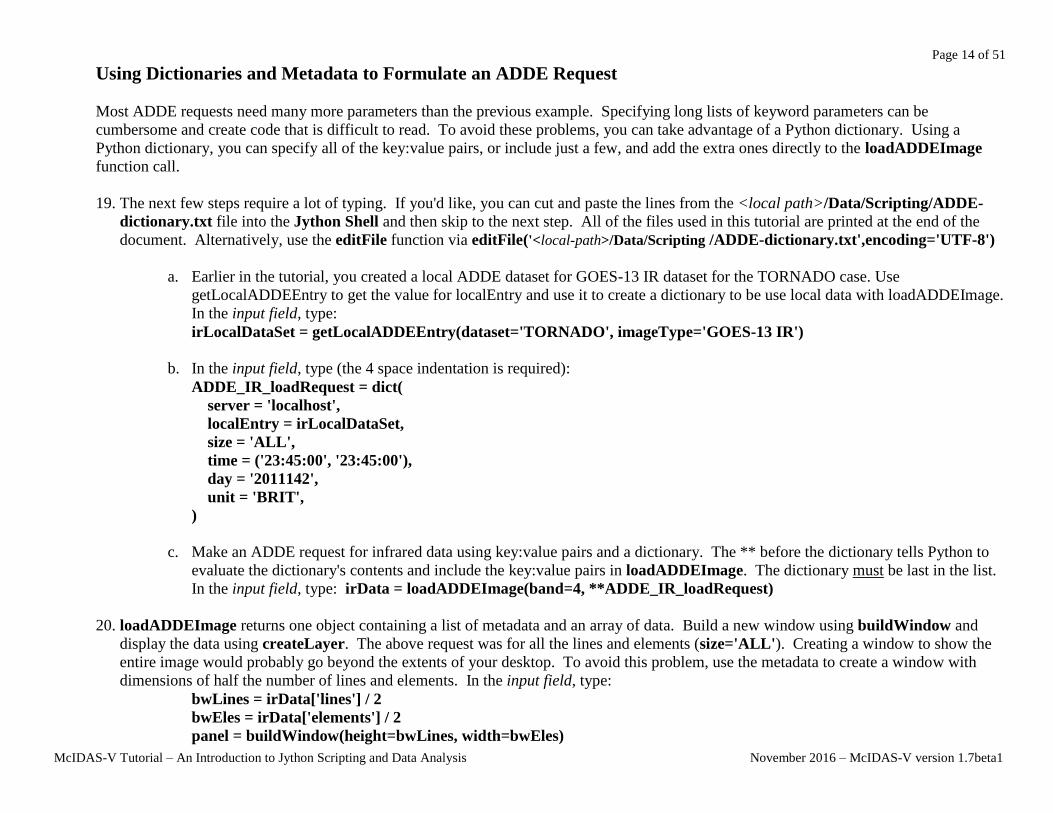
Using Dictionaries and Metadata to Formulate an ADDE Request
Most ADDE requests need many more parameters than the previous example. Specifying long lists of keyword parameters can be
cumbersome and create code that is difficult to read. To avoid these problems, you can take advantage of a Python dictionary. Using a
Python dictionary, you can specify all of the key:value pairs, or include just a few, and add the extra ones directly to the loadADDEImage
function call.
19. The next few steps require a lot of typing. If you'd like, you can cut and paste the lines from the <local path>/Data/Scripting/ADDE-
dictionary.txt file into the Jython Shell and then skip to the next step. All of the files used in this tutorial are printed at the end of the
document. Alternatively, use the editFile function via editFile('<local-path>/Data/Scripting /ADDE-dictionary.txt',encoding='UTF-8')
a. Earlier in the tutorial, you created a local ADDE dataset for GOES-13 IR dataset for the TORNADO case. Use
getLocalADDEEntry to get the value for localEntry and use it to create a dictionary to be use local data with loadADDEImage.
In the input field, type:
irLocalDataSet = getLocalADDEEntry(dataset='TORNADO', imageType='GOES-13 IR')
b. In the input field, type (the 4 space indentation is required):
ADDE_IR_loadRequest = dict(
server = 'localhost',
localEntry = irLocalDataSet,
size = 'ALL',
time = ('23:45:00', '23:45:00'),
day = '2011142',
unit = 'BRIT',
)
c. Make an ADDE request for infrared data using key:value pairs and a dictionary. The ** before the dictionary tells Python to
evaluate the dictionary's contents and include the key:value pairs in loadADDEImage. The dictionary must be last in the list.
In the input field, type: irData = loadADDEImage(band=4, **ADDE_IR_loadRequest)
20. loadADDEImage returns one object containing a list of metadata and an array of data. Build a new window using buildWindow and
display the data using createLayer. The above request was for all the lines and elements (size='ALL'). Creating a window to show the
entire image would probably go beyond the extents of your desktop. To avoid this problem, use the metadata to create a window with
dimensions of half the number of lines and elements. In the input field, type:
bwLines = irData['lines'] / 2
bwEles = irData['elements'] / 2
panel = buildWindow(height=bwLines, width=bwEles)

Page 15 of 51
McIDAS-V Tutorial – An Introduction to Jython Scripting and Data Analysis November 2016 – McIDAS-V version 1.7beta1
21. Now create layer objects for the infrared data. Use createLayer with the object irData. In the input field, type:
irLayer = panel[0].createLayer('Image Display', irData)
22. Apply the 'Longwave Infrared Deep Convection' color table to the infrared layer. Since there is a unique name for each color table, the
syntax is a little different than that used with setProjection, and the entire naming structure is not necessary here. In the input field, type:
irLayer.setEnhancement('Longwave Infrared Deep Convection')
23. Using the values from the keywords 'sensor-type' and 'nominal-time' from the irData object, create a string to use with setLayerLabel
(remember that the 4 spaces of indentation are mandatory).
a. Print the list of keys included in the irData object. In the input field, type:
print irData.keys( )
b. In the input field, type:
irLabel = '%s %s' % (
irData['sensor-type'],
irData['nominal-time']
)
c. In the input field, type:
irLayer.setLayerLabel(label=irLabel, size=16, color='White', font='SansSerif')
c. After checking the new layer label in the buildWindow Display, close the window.
Functions in Python
Functions are a way to refer to a piece of code that takes arguments and returns results based on those arguments. Functions are the key to
creating reusable code and avoiding repetition, and Python makes them easy to define and use. The next sections utilize functions in
McIDAS-V. In Python, defining functions is straightforward.
24. Create a function named add and demonstrate its usage with numbers and letters. Hopefully, 2 plus 2 will equal 4. As with loops and
if/else blocks, indentation/dedent indicate the end of the function. In the input field, type:
def add(a, b):
return a+b
print add(2,2)

Page 16 of 51
McIDAS-V Tutorial – An Introduction to Jython Scripting and Data Analysis November 2016 – McIDAS-V version 1.7beta1
25. Similar to IDL but unlike languages like C and FORTRAN, Python functions do not need to explicitly state the type of argument.
Consequences of this can be observed when attempting to use something other than numbers with the add function. In the input field,
type:
print add('a', 'b') Click Evaluate.
This code results in:
ab
This still works. The + operator works just as well on 'a' and 'b' as it does on 1 and 2, so the function completes without error.
Jython Library
26. The above exercises used functions such as setLayerLabel and loadADDEImage. The code for these functions can be found in the
Jython Library. Open the Jython Library and search for code to set a layer label.
a. In Main Display, select Tools -> Formulas -> Jython Library.
b. Open the System -> Background Processing Functions library.
c. Using the search utility type setLayerLabel. This shows you the code that sets a layer label. Keep pressing Enter or use the
up/down arrows to search for multiple instances of setLayerLabel in the library.
Note that users can share code by adding functions to the Local Jython Library. An example of this will be covered later in this tutorial.
Using Functions in a McIDAS-V Script
Building upon the previous examples, the next script uses the importEnhancement, mask and mul functions. mask and mul are system
functions, packaged with McIDAS-V.
The <local-path>/Data/Scripting/function.py file is an example script showing how to use these functions and ways to make the script
platform independent. These are not to be entered into the Jython Shell at this time. Read through the following portions of the script and
the associated comments to learn what the script is doing at each step.

Page 17 of 51
McIDAS-V Tutorial – An Introduction to Jython Scripting and Data Analysis November 2016 – McIDAS-V version 1.7beta1
The first line of the code imports common functions in the os library. These functions are used to create platform-independent path names.
import os
#
# Setting up a variable to specify the location of your final images
# makes your script easier to read and more portable when you share it
# with other users
#
homePath = expandpath('~')
dataPath = os.path.join(homePath, 'Data')
scriptingPath = os.path.join(dataPath, 'Scripting')
enhancementPath = os.path.join(scriptingPath, 'Color-Enhancements')
areaPath = os.path.join(scriptingPath, 'tornado-areas')
irPath = os.path.join(areaPath, 'IR')
#
# imagePath is the directory to store final images
# and/or animated gif files
#
imagePath = os.path.join(scriptingPath, 'Images')
The GOES-13 IR TORNADO dataset is used, this time with temperature (unit='TEMP') values requested:
#
# This example gets the information from the dataset created previously in the tutorial
#
irLocalDataSet = getLocalADDEEntry('TORNADO','GOES-13 IR')
ADDE_IR_loadRequest = dict(
debug=True,
server='localhost',
localEntry=irLocalDataSet,
size='ALL',
time=('23:45:00','23:45:00'),
day='2011142',
unit='TEMP',
)
irData = loadADDEImage(**ADDE_IR_loadRequest)

Page 18 of 51
McIDAS-V Tutorial – An Introduction to Jython Scripting and Data Analysis November 2016 – McIDAS-V version 1.7beta1
The mask function requires a temperature threshold:
#
# assign a temperature threshold used with mask() function
#
temperatureThreshold = 250.0
Applying a mask requires a two part process. First, a threshold temperature is applied to the data object returned from loadADDEImage,
creating a new data object of either values of 1's or missing. Second, the original data object is multiplied by the new data object. The data
object created by the mul function creates a data object that contains either temperature or missing values.
#
# Applying a mask is a two part process.
# First we assign a value of 1 or missing value to a temporary data object
# Second, multiply the first results to the temporary data object
#
maskedData = mask(irData, 'lt', temperatureThreshold, 1)
finalDataSet = mul(irData, maskedData)
The importEnhancement function reads in a file exported using the color table editor. The name of the color table is extracted and used
with setEnhancement:
#
# Import enhancement table
#
IRColorTableFile = os.path.join(enhancementPath, 'Tornado-IR.xml')
IRTable = importEnhancement(IRColorTableFile)
IRTableName = IRTable.getName()
As previously done, the last section of the script builds a window, creates the layer, applies the enhancement table and sets the projection.
#
# Build a window
#
bwLines = irData['lines'] / 2
bwEles = irData['elements'] / 2
panel = buildWindow(height=bwLines, width=bwEles)
panel[0].setWireframe(False)
#
# Add layers to the existing window set enhancement table and data ranges
#
irLayer = panel[0].createLayer('Image Display', finalDataSet)
irLayer.setLayerLabel('GOES-13 Temperatures less than ' + str(temperatureThreshold) + ' %timestamp%')

Page 19 of 51
McIDAS-V Tutorial – An Introduction to Jython Scripting and Data Analysis November 2016 – McIDAS-V version 1.7beta1
irLayer.setEnhancement(IRTableName, range=(temperatureThreshold,200))
#
# Set the center latitude, longitude and scale
#
panel[0].setProjection('US>States>N-Z>Oklahoma')
panel[0].setCenter(33, -97, scale=.5)
fileName=os.path.join(imagePath, 'ir-image.gif')
panel[0].captureImage(fileName)
27. From the Jython Shell, run function.py. In the input field, type:
editFile('<local-path>/Data/Scripting/function.py',encoding='UTF-8')
28. Evaluate the function.py file by clicking Evaluate.
29. Open a browser and view the file '<local-path>/Data/Scripting/Images/ir-image.gif'.
30. Close the display window created by the function.py script.
Creating Movies in a McIDAS-V Script
In the previous example, you created a single image. You can also create movies that contain loops of images. To do this, multiple data
requests must be made. The <local-path>/Data/Scripting/image-movie.py file is an example of the creation of movie loops in McIDAS-V.
In this example, the loop is created by making a call to listADDEImageTimes and multiple calls to loadADDEImage.
listADDEImageTimes is similar to listADDEImages, but returns a list of dictionaries containing only image days and times. Below is part
of the script with some comments. These are not to be entered into the Jython Shell at this time.
A Python list, as described previously, is used to store data objects and is initialized using the syntax below. As the script loops through
loadADDEImage calls, the data objects returned are appended to the list. In this script, myLoop is the Python list:
myLoop=[]
listADDEImageTimes uses the dictionary parms as its input parameters. The dictionary object dateTimeList is returned and contains
keyword/value pair for each day and time.
dateTimeList = listADDEImageTimes(**parms)

Page 20 of 51
McIDAS-V Tutorial – An Introduction to Jython Scripting and Data Analysis November 2016 – McIDAS-V version 1.7beta1
The script then loops through all the dictionaries returned from the call to listADDEImageTimes. Using a for loop, individual directories,
dateTime, are extracted from the list dictionaries, dateTimeList, which was returned from listADDEImageTimes. The loop takes the time
value out of the dateTime dictionary which is used to create a new dictionary that is passed into loadADDEImage.
for dateTime in dateTimeList:
imageTime = dateTime['time']
ADDE_IR_loadRequest = dict(
localEntry=irLocalDataSet,
day=dateTime['day'],
time=(imageTime,imageTime),
band=4,
unit='TEMP',
size='ALL'
)
IRData = loadADDEImage(**ADDE_IR_loadRequest)
maskedData = mask(irData, ‘lt’, temperatureThreshold, 1)
finalDataSet = mul(irData, maskedData)
The data objects returned from listADDEImageTimes and passed through mask and mul are added to myLoop using the append method.
myLoop.append(finalDataSet)
Once the loop is completed, a window is built and myLoop is used to create an Image Sequence Layer which is saved as an animated gif.
bwLines = irData[‘lines’] / 2
bwEles = irData[‘elements’] / 2
panel = buildWindow(height=bwLines, width=bwEles)
panel[0].setWireframe(False)
irLayer = panel[0].createLayer('Image Sequence Display' ,myLoop)
fileName = os.path.join(imagePath, 'ir-loop.gif')
writeMovie(filename,globalPalette=False)
31. From the Jython Shell run image-movie.py. In the input field, type:
editFile('<local path>/Data/Scripting/image-movie.py',encoding='UTF-8')
32. Evaluate the image-movie.py file by clicking Evaluate.
33. Open a browser and view the file '<local-path>/Data/Scripting/Images/ir-loop.gif'.

Page 21 of 51
McIDAS-V Tutorial – An Introduction to Jython Scripting and Data Analysis November 2016 – McIDAS-V version 1.7beta1
Creating Your Own McIDAS-V Script
34. You now have all the tools necessary to write a script that creates a movie of the infrared images placed over a basemap. For this exercise,
a. import the enhancement table from <local-path>/Data/Scripting/Color-Enhancements/Tornado-basemap.xml
b. write a script that does the tasks listed below:
1. uses the local data files from the TORNADO 'GOES-13 IR' dataset
2. creates and uses the local McIDAS Area dataset for a base map
a. name the dataset TORNADO
b. assign the image type 'Land Sea Mask'
c. data is located <local-path>/Data/Scripting/tornado-areas/BASE
3. uses the entire size of the image of both datasets
4. loads a list IR temperature data that spans 14:45 on day 2011142 to and 02:45 on day 2011143
a. the mask function removes temperature greater than 250 K
b. uses the enhancement table <local-path>/Data/Scripting/Color-Enhancements/Tornado-IR.xml
c. applies the color enhancement with a range of 250 to 200 K
5. loads a single base map image and uses the enhancement table:
<local-path>/Data/Scripting/Color-Enhancements/Tornado-basemap.xml
6. builds a window 700 lines X 1000 elements
7. creates an Image Display layer from the base map dataset (do not include the layer label)
8. overlays an Image Sequence Display layer from the IR data list
9. adds a layer label to the IR data set which includes
a. the text 'Joplin Tornado'
b. timestamp
c. displayname
10. sets the projection to Central U.S.
11. changes the center point to 35N 97W with a scale factor of 1.5
12. turns off the wireframe box
13. adds the annotation 'Joplin, Missouri'; text is left and center justified at 37.15N and 94.5W
14. saves the movie with the file name of <local-path>/Data/Scripting/Images/image-exercise.gif
An example solution is available at <local path>/Data/Scripting/image-exercise.py. However, before checking the solution, it is
recommended that you try to complete the tasks on your own.

Page 22 of 51
McIDAS-V Tutorial – An Introduction to Jython Scripting and Data Analysis November 2016 – McIDAS-V version 1.7beta1
Running Scripts from a Command Prompt
So far in this tutorial, you have been running commands and scripts using the Jython Shell. Scripts can also be run from the command line
by adding the flag -script to the startup script.
35. Run the McIDAS-V script using the –script flag.
a. Exit McIDAS-V.
b. Open a terminal and change directory to the directory where McIDAS-V is installed (<user-path>/McIDAS-V-System)
c. Run the <local-path>/Data/Scripting/image-exercise.py script.
For Unix, type:
./runMcV –script <local-path>/Data/Scripting/image-exercise.py
For Windows, type:
runMcV.bat –script <local-path>/Data/Scripting/image-exercise.py
d. The progress of the script can be monitored by watching the mcidasv.log file in your McIDAS-V directory with the tail
command.
Type: tail -f <user-path>/McIDAS-V/mcidasv.log
e. From your browser, view the file <local-path>/Data/Scripting/Images/image-exercise.gif that was created from
<local-path>/Data/Scripting/image-exercise.py.

Page 23 of 51
McIDAS-V Tutorial – An Introduction to Jython Scripting and Data Analysis November 2016 – McIDAS-V version 1.7beta1
Introduction to Data Manipulation in McIDAS-V
This section of the tutorial will use the term “VisAD data object.” A VisAD data object contains the data as well as detailed information
about a data’s structure and type. These objects can also contain units, temporal and geospatial information. In this section of the tutorial, an
introduction to the VisAD data object is presented as well as a general introduction to accessing the information within the data object.
36. Restart McIDAS-V and load the '<local-path>/Data/Scripting/load_grid.py' script provided with this tutorial into the Jython Shell
(Tools -> Formulas -> Jython Shell). In the input field of the Jython Shell, type:
editFile('<local-path>/Data/Scripting/load_grid.py', encoding='UTF-8')
Click Evaluate (or Shift+Enter) to load the script into the Jython Shell.
Click Evaluate again to execute the script.
37. Use the standard Jython function type() to display the class of the data contained in h8b1:
print type(h8b1) Click Evaluate.
The h8b1 object belongs to a class called “MappedGeoGridFlatField.” This class is returned when data is loaded via the loadGrid()
function.
38. The Jython built-in type function does not describe how the data is structured. The JPythonMethod library built into McIDAS-V contains
a function called “whatTypes()”. This function describes the structure of any VisAD data object. whatTypes can be used for debugging.
In the input field of the Jython Shell, type:
print whatTypes(h8b1)
Click Evaluate.
The h8b1 object domain contains latitude and longitude coordinates. The latitude and longitude coordinate unit is “degrees”. The
range of the h8b1 data object contains the data. In this case, the data are values of albedo. Albedo has no unit (Unit: 1).
39. View the data mapping. Type: print getType(h8b1)
The result, ((Longitude, Latitude) -> albedo[unit:1]), displays a map of the albedo data (stored in the range) to the longitude (stored in
domain[0]) and latitude coordinates (stored in domain[1]).

Page 24 of 51
McIDAS-V Tutorial – An Introduction to Jython Scripting and Data Analysis November 2016 – McIDAS-V version 1.7beta1
40. Determine the size of the data and range of the coordinates. In the Jython Shell, type:
h8ds = getDomainSet(h8b1); print h8ds
Click Evaluate.
The semicolon ( ; ) links the commands together. In this way, multiple commands can be entered on one line, and executed in
sequence. This output can be interpreted with the help of other commands run earlier. In the previous steps, evaluating the
whatTypes() function showed that the domain index for the longitude coordinate is 0 and the latitude coordinate is 1. This can also be
inferred from the getType() command. Therefore, in the output of getDomainSet(), Dimension 0 is longitude which has a range of
124.242645 to 125.749756, and Dimension 1 is latitude which has a range of 35.063034 to 36.36338. The getDomainSet() output
also shows that the length, or number of data points in this data are 441. If a user should use len(h8b1), the length of the
MappedGeoGridFlatField metadata is returned.
41. Once the data object domain set of a data object is retrieved (remember, this is the set of latitude and longitude coordinates), the latitude
and longitude values for each grid point can be accessed. Using the variable h8ds created in the previous step, type:
h8latlons = getLatLons(h8ds)
h8lats = h8latlons[0]
h8lons = h8latlons[1]
Note: The JPythonMethod getLatLons resets the order of the longitude and latitude coordinates. This means that the latitude values
are always returned in the zero index, and the longitudes are always returned as the first index. To get return the shape of the
h8latlons array, type:
import Numeric
print Numeric.shape(h8latlons)
Note: McIDAS-V’s see function allows for printing out all of the different options with Numeric. To do this, type:
print see(Numeric)
42. Print the first four latitude points. Note: In the Jython Shell, it is a good practice to limit the size of data printed. Type:
print h8lats[0:4]

Page 25 of 51
McIDAS-V Tutorial – An Introduction to Jython Scripting and Data Analysis November 2016 – McIDAS-V version 1.7beta1
43. Additional methods for working with this data can be found in JPythonMethods (http://www.ssec.wisc.edu/visad-
docs/javadoc/visad/python/JPythonMethods.html). For example, a method to return the min/max of the data is getMinMax(). In the
Jython Shell, type:
print getMinMax(h8b1)
This method returns that the range of albedo values in h8b1 goes from a minimum value of ~0.234 to a maximum value of ~0.553.
44. An additional JPythonMethod, getValues(), can be used to return the data points as float values. The values returned can be saved to a
variable named myData. In the Jython Shell, type:
myData = getValues(h8b1)
a. Determine the type of myData. In the Jython Shell, type:
print type(myData)
The type returned is an array.
b. What is the length of the myData array? Does it match the length found in the domain set? In the Jython Shell, type:
print len(myData)
The length is 1. This does not match the length found in the domain set in the
next command.
c. What is the length of myData[0]? In the Jython Shell, type:
print len(myData[0])
The length is 441, which should match the length reported in
getDomainSet(h8b1) above. The actual shape of this array is a 1x441.
Therefore, the first len() returns the length of the first dimension of the array
myData. In this case, since there is only one timestamp in the file, that length
is 1. This is similar to a Fortran array of REAL myData(1,441). An
alternative way of returning the shape of the array would be to run:
print Numeric.shape(myData)

Page 26 of 51
McIDAS-V Tutorial – An Introduction to Jython Scripting and Data Analysis November 2016 – McIDAS-V version 1.7beta1
Creating Functions for the Jython Library
In this section, a function called probe will be created, which can be expanded to load multiple channels from the Himawari-8 satellite.
Later, these data will be used in a cloud algorithm. The goal of this section is to provide the user with the knowledge base that will enable
them to create their own functions to meet their research needs.
45. Using the Jython Library, create a new function called probe().
a. In the Main Display, select Tools -> Formulas -> Jython Library to open the Jython Library.
b. In the left panel of the Jython Library, select Local Jython -> User’s Library. The right panel of the Jython Library is the
location where new functions are defined.
c. Create a new function in the Training Library. Expand Local Jython and select Training Library (this library was created in
the An Introduction to Jython Scripting tutorial. If one does not exist, select Local Jython and then File -> New Jython
Library and enter Training Library). Left-Click in the right panel of the Jython Library. Type: def probe():
This defines a new function called probe(). This function will require three input parameters: the data object (2D lat/lon flat
field of data), the latitude location, and the longitude location. Modify the definition line to include the input parameters. The
final structure of the definition line should be: def probe(field, lat, lon):
This function returns the data value at the input latitude/longitude. Next, add a return statement: return valueAtLocation
In Jython, a code block is defined by consistent indention. In this example, code block indentation will be four spaces. The
two lines of the code block should now be:
def probe(field, lat, lon):
return valueAtLocation
d. Two McIDAS-V libraries are needed for this function. Add import statements to the code block between the definition line
and the return line:
def probe(field, lat, lon):
from ucar.unidata.data.grid import GridUtil
from visad.georef import EarthLocationTuple
return valueAtLocation

Page 27 of 51
McIDAS-V Tutorial – An Introduction to Jython Scripting and Data Analysis November 2016 – McIDAS-V version 1.7beta1
e. Add code to retrieve data value at input lat/lon point:
altitude = 0.0
loc = EarthLocationTuple(lat, lon, altitude)
valueAtLocation = GridUtil.sampleToReal(field, loc, None)
The completed probe() function is:
def probe(field, lat, lon):
from ucar.unidata.data.grid import GridUtil
from visad.georef import EarthLocationTuple
altitude = 0.0
loc = EarthLocationTuple(lat, lon, altitude)
valueAtLocation = GridUtil.sampleToReal(field, loc, None)
return valueAtLocation
f. Select Save and close the Jython Library.
Preparing to Test the probe() Function by Blending Interactive and Scripting Methods
46. The Jython method, os.path.join is used in the following sequence, if the Jython “os” module has not already been imported, import it
now. In input field of the Jython Shell, type: import os
47. Load the TORNADO/GOES-13 IR data from the local dataset into the Field Selector via the interactive Data Chooser. Display the data
using the McIDAS-V scripting API.
a. Bring the Main Display forward. In the Jython Shell, type:
activeDisplay().toFront()
b. Click the button on the Main Toolbar to bring the Data Explorer to the front.
c. In the Data Explorer, open the Data Sources tab.

Page 28 of 51
McIDAS-V Tutorial – An Introduction to Jython Scripting and Data Analysis November 2016 – McIDAS-V version 1.7beta1
d. Using the Satellite -> Imagery chooser, load the <LOCAL-DATA> created in previous step (Dataset: TORNADO, Image
Type: GOES-13 IR). In the Relative tab, select the 5 most recent times and click Add Source. Additional instructions for
loading satellite imagery can be found under Choosing Satellite Imagery in the User’s Guide or the Satellite Imagery Tutorial.
e. When the Joplin data is in the Field Selector, click the Jython Shell (or select Tools -> Formulas -> Jython Shell) to bring
the Jython Shell forward.
f. The Joplin data will be selected from the Jython Shell, and used to test the probe() function. In the input field of the Jython
Shell type:
joplin = selectData('ir')
g. Click Evaluate. Note: The Field Selector title is “ir.” The title matches the string entered in the selectData() call.
h. In the secondary Field Selector window, select the GOES-13 IR -> 10.7 um IR Surface/Cloud-top Temp -> Temperature
data source.
i. Once the bottom Times tab in the window becomes visible, click OK.
j. Create a grid table display of the Joplin data. Type:
panel = buildWindow()
panel[0].createLayer('Grid Table', joplin[0])
48. Notice the section of data displayed in the grid table with no latitude or longitude and a value of 0 for Band4_TEMP_0. These are points
in the area that are not navigated on the earth.
a. At the top of the Layer Controls turn on the option for Show native coordinates. Now, instead of seeing invalid latitude and
longitude values, image element and image lines are listed. This demonstrates that while there are data points without a
latitude and longitude, there are points included in the AREA file.
b. Once done interrogating the chart, turn Show native coordinates off.
49. For analysis and sometimes display purposes, these points can be set to "Missing". In the Jython Shell type:
joplinMiss = setMissingNoNavigation(joplin[0])
panel[0].createLayer('Grid Table', joplinMiss)
Notice the values are now or (dependent on your platform), corresponding to a missing value.

Page 29 of 51
McIDAS-V Tutorial – An Introduction to Jython Scripting and Data Analysis November 2016 – McIDAS-V version 1.7beta1
Exercise 1: Test the probe() function:
a. Select five navigated points from the Grid Table display. Write the five test points in the table below:
Latitude Longitude Data
Value
b. Test the probe function on the five points by using each lat/lon value pair in the function call. In the Jython Shell, type:
print probe(joplinMiss, <latitude>, <longitude>)
c. Determine the class of joplin and joplin[0] using print type(). In the Jython Shell, type:
print type(joplin)
print type(joplin[0])
Data Object Belongs to class
joplin
joplin[0]

Page 30 of 51
McIDAS-V Tutorial – An Introduction to Jython Scripting and Data Analysis November 2016 – McIDAS-V version 1.7beta1
d. Using the getType method (object.getType()), inspect the data mapping of joplin and joplin[0]. Write the mapping in the
space below. In the Jython Shell, type:
print getType(joplin)
print getType(joplin[0])
e. Use the getImageTimes() method on joplin. In the Jython Shell, type:
print joplin.getImageTimes()
Note, the solution to Exercise 1 can be found on the next page.
Extra: Using the describe() function, type:
print describe(joplin[0])
This function is meant to show quick statistics for a flatField or multiple flat fields. If you have questions, comments, requests for additional
functionality or bug reports, please post them to the Scripting Forum.
It is possible to calculate statistics on any array, provided it is converted to a VisAD field:
myField = field([1, 2, 3, 4, 5, 9, 9, 9, 9])
print describe(myField)

Page 31 of 51
McIDAS-V Tutorial – An Introduction to Jython Scripting and Data Analysis November 2016 – McIDAS-V version 1.7beta1
Exercise 1 Solution: Test the probe() function:
a. Select five navigated points from the Grid Table display. Write the five test points in the table below:
Latitude Longitude Data Value
53.2 -65.912 276.3
This chart contains one sample latitude/longitude/data point to demonstrate an example solution.
b. Test the probe function on the five points by using each lat/lon value pair in the function call. In the Jython Shell, type:
print probe(joplinMiss, 53.2, -65.912) This returns a value of 276.3, matching the grid table output.
c. Determine the class of joplin and joplin[0] using print type(). In the Jython Shell, type:
print type(joplin)
print type(joplin[0])
Data Object Belongs to class
joplin visad.meteorology.ImageSequenceImpl
joplin[0] visad.metrorology.NavigatedImage
d. Using the getType method (object.getType()), inspect the data mapping of joplin and joplin[0]. Write the mapping in the space
below. In the Jython Shell, type: print getType(joplin)
(Time -> ((ImageElement, ImageLine) -> Band4_TEMP))
The joplin data object is an image sequence, so this shows the time domain (which could be multiple times) linked to the data coordinates.
Type: print getType(joplin[0])
((ImageElement, ImageLine) -> Band4_TEMP)
The joplin[0] data object is the navigated image, this reveals that the image has element and line coordinates mapped to the data.
e. Use the getImageTimes() method on joplin. In the Jython Shell, type: print joplin.getImageTimes()
This step emphasizes the point that the image sequence data object joplin is an image sequence and the times can be extracted as a list.

Page 32 of 51
McIDAS-V Tutorial – An Introduction to Jython Scripting and Data Analysis November 2016 – McIDAS-V version 1.7beta1
Scripting Exercise: Build a Himawari-8 Cloud Mask (Comprehensive Exercise)
Using loadGrid, the Jython Library, and knowledge of the VisAD data object, build a simple cloud mask algorithm for Himawari-8’s AHI
sensor. This exercise will extend your knowledge of the VisAD data model by using methods to extract raw data arrays from VisAD data
objects and operate on the data arrays in a way that is familiar to users already comfortable with programming languages like MATLAB® or
Fortran.
First, explore a Himawari-8 scene interactively and determine cloud/no-cloud thresholds for various AHI channels. Next, add the outline of a
Jython cloud mask function provided to your Jython Library. Implement the algorithm of the cloud mask Jython function with the
thresholds determined interactively. Finally, run the algorithm as many times as needed while exploring the results. Iterate between
interactively assessing thresholds and algorithm development until you are satisfied with the cloud mask.
50. Load Himawari-8 bands interactively and determine cloud thresholds. The Himawari-8 data distributed with this tutorial is split into a
single band per file. For example, band 3 contains the string “B03” at the end of the filename. Create a data source per band you are
interested in.
a. Add a data source for band 1.
1. In the Data Explorer, open the Data Sources tab and navigate to the Gridded Data -> Local chooser.
2. Under Data Type, select “Grid files (netCDF/GRIB/OPeNDAP/GEMPAK)”.
3. Navigate to ‘<local path>/Data/Scripting/ H8’ and Double-Click the file
HS_H08_20150715_0100_B01_FLDK_subset.nc.
b. Repeat step 50a for other bands of interest. Add a data source for at least three more bands, including band 3 (high resolution
visible channel), band 9 (a channel with high water vapor absorption), and band 14 (an infrared window channel).
c. Display the data for band 1.
1. Create a new one panel map tab in the Main Display window.
2. In the Data Sources panel of the Field Selector, select the top HS_H08* data source. The order of the data sources in this
panel is determined by the order they were added. Since band 1 was added first in step 51a, this is at the top of the list.
3. Choose the Plan Views -> Color-Shaded Plan View display type and click Create Display.
d. Create a Data Probe/Time Series display for all data sources created in steps 51a and 51b.
1. In the Data Sources panel of the Field Selector, select the top HS_H08* (band 1) data source. Choose the Data

Page 33 of 51
McIDAS-V Tutorial – An Introduction to Jython Scripting and Data Analysis November 2016 – McIDAS-V version 1.7beta1
Probe/Time Series display type.
2. Click Create Display.
3. To avoid confusion as more layers are added to the display, change the parameter name below the chart from albedo to
Band 1. To do this, Right-Click on albedo below the chart and choose Parameter albedo -> Chart Properties. In the
Properties window, set the Legend Label field to be Band 1and click OK. An alternative way of getting to the
Properties window for a layer in the chart is to Double-Click on the parameter.
e. Add the other fields added in step 51b to the Data Probe/Time Series display. In the Layer Controls of the Data Probe/Time
Series display, Left-Click on the Band 1 data readout line to select the line.
1. Once the line is highlighted, Right-Click to select Add Parameter....
2. Use the secondary Field Selector select the other fields, clicking Add Selected>> after each addition.
3. When all the desired fields have been added to the panel below Add Selected>> click OK.
4. Repeat the last step in 51d to set the parameter name of each field to be the band number.
51. Explore the scene. Using the Data Probe (hold down the middle mouse button over the display) and the Data Probe/Time Series display,
write down a cutoff value that is representative of the transition from not cloudy to cloudy. This is just to get started – clearly, you won’t
find a single value for a single channel that works perfectly for the entire scene.
52. Copy the script ‘<local-path>/Data/UserFunctions/ahi_cloudmask.py’ to the Jython Library. This is the outline of a cloud mask script
that can be improved in later steps. Try running the cloud mask provided without modification:
a. Open ahi_cloudmask.py in a text editor.
b. In McIDAS-V, click Tools -> Formulas -> Jython Library.
c. Create a new Jython Library by selecting File->New Jython Library from the menu. Enter AHI-cloudmask and click OK.
d. Open the Local Jython -> AHI-cloudmask library. Copy and paste the text in ahi_cloudmask.py from the text editor into the
library and click Save.
e. Open the Jython Shell (click Tools -> Formulas -> Jython Shell) and type:
run_ahi_cloudmask() Click Evaluate.
You should get a new display showing a cloud mask, but at this point it is pretty bad! It misses most of the clouds in the scene.

Page 34 of 51
McIDAS-V Tutorial – An Introduction to Jython Scripting and Data Analysis November 2016 – McIDAS-V version 1.7beta1
53. Modify the cloud mask function to implement the thresholds you determined in step 52:
a. In the Jython Library, examine the ahi_cloudmask() code pasted in the previous step. The code locates the AHI data on the
disk, loads it into McIDAS-V with loadGrid, and then organizes it by band number in a Python dictionary for easy access.
For the purposes of this exercise, the focus will be on the function do_cloudmask (ahi_cloudmask.py line 109), which
implements the cloud mask algorithm. The outline of this function is already implemented; it is up to the user to fill in the
cloud/no-cloud thresholds determined in step 52.
b. Now, implement your cloud mask. The portion of the script you will work on is labeled “You can fill in additional
clear/cloudy tests here”. Directly above this comment, there are two tests already implemented, one for band 14 and another
for band 1. These tests use the function mask from JPythonMethods to create a simple cloud/no-cloud mask based on
brightness temperature or reflectance threshold. Modify these two tests with the thresholds determined for band 1 and band 14
in previous steps. For example, assuming you wrote down a threshold of 260K for band 14, change the line:
threshold_mask = mask(ahi_datas[14], 'gt', 220.0, False)
to
threshold_mask = mask(ahi_datas[14], 'gt', 260.0, False)
c. Now, copy the block labeled “Test number 2” (line 123), and paste it directly below. Change the comment to “Test number
3”, change the dictionary key to the next channel you would like to work on, and change the threshold as desired. Note that
line 152 (the list of bands) will need to be updated to include the new bands being worked with, bands 3 and 9.
d. Redo the previous step to implement all the thresholds you determined.
e. Once all of the cloud mask tests have been added to the library, click Save at the bottom of the Jython Library.
f. In the Jython Shell, rerun run_ahi_cloudmask() and examine the results. Has your cloud mask improved?
g. These brightness temperature and reflectance threshold tests are simple to define and run quickly because they can be
implemented with built-in functions like mask that operate on an entire VisAD data object in a single function call. You may
ask: what if I have an algorithm that cannot be expressed using functions from JPythonMethods? For example, cloudy areas
are often more spatially heterogeneous than cloud-free areas and decide you want to develop a test that considers the standard
deviation of neighboring pixels as a simple measure of spatial heterogeneity.
To illustrate this, the file ahi_cloudmask.py has already implemented a function called do_std_dev_test, but it is initially
unused by do_cloudmask. As the first step, modify do_cloudmask to use do_std_dev_test. This part is simple because
do_std_dev_test returns a VisAD Data object (similar to what is returned by mask) that can be multiplied by the current
cloud mask result to obtain the combined cloud mask (see line 132):
Page 35 of 51
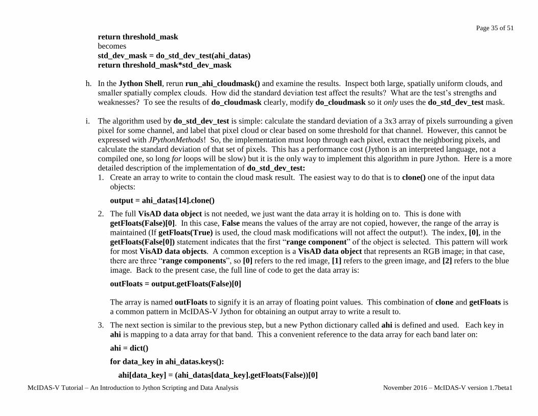
McIDAS-V Tutorial – An Introduction to Jython Scripting and Data Analysis November 2016 – McIDAS-V version 1.7beta1
return threshold_mask
becomes
std_dev_mask = do_std_dev_test(ahi_datas)
return threshold_mask*std_dev_mask
h. In the Jython Shell, rerun run_ahi_cloudmask() and examine the results. Inspect both large, spatially uniform clouds, and
smaller spatially complex clouds. How did the standard deviation test affect the results? What are the test’s strengths and
weaknesses? To see the results of do_cloudmask clearly, modify do_cloudmask so it only uses the do_std_dev_test mask.
i. The algorithm used by do_std_dev_test is simple: calculate the standard deviation of a 3x3 array of pixels surrounding a given
pixel for some channel, and label that pixel cloud or clear based on some threshold for that channel. However, this cannot be
expressed with JPythonMethods! So, the implementation must loop through each pixel, extract the neighboring pixels, and
calculate the standard deviation of that set of pixels. This has a performance cost (Jython is an interpreted language, not a
compiled one, so long for loops will be slow) but it is the only way to implement this algorithm in pure Jython. Here is a more
detailed description of the implementation of do_std_dev_test:
1. Create an array to write to contain the cloud mask result. The easiest way to do that is to clone() one of the input data
objects:
output = ahi_datas[14].clone()
2. The full VisAD data object is not needed, we just want the data array it is holding on to. This is done with
getFloats(False)[0]. In this case, False means the values of the array are not copied, however, the range of the array is
maintained (If getFloats(True) is used, the cloud mask modifications will not affect the output!). The index, [0], in the
getFloats(False[0]) statement indicates that the first “range component” of the object is selected. This pattern will work
for most VisAD data objects. A common exception is a VisAD data object that represents an RGB image; in that case,
there are three “range components”, so [0] refers to the red image, [1] refers to the green image, and [2] refers to the blue
image. Back to the present case, the full line of code to get the data array is:
outFloats = output.getFloats(False)[0]
The array is named outFloats to signify it is an array of floating point values. This combination of clone and getFloats is
a common pattern in McIDAS-V Jython for obtaining an output array to write a result to.
3. The next section is similar to the previous step, but a new Python dictionary called ahi is defined and used. Each key in
ahi is mapping to a data array for that band. This a convenient reference to the data array for each band later on:
ahi = dict()
for data_key in ahi_datas.keys():
ahi[data_key] = (ahi_datas[data_key].getFloats(False))[0]

Page 36 of 51
McIDAS-V Tutorial – An Introduction to Jython Scripting and Data Analysis November 2016 – McIDAS-V version 1.7beta1
4. Next, iterate through each pixel. We use the Python function enumerate to get a reference to both the index i and the
value of the image at i (hereafter, the value of the image at the index i will be called pixel):
for i, pixel in enumerate(outFloats):
5. Next, the standard deviation tests are done. For each pixel, extract the surrounding 3x3 pixels using a helper function
called get_3x3. VisAD internally represents all data as a 1-dimensional array, so the dimensionality must be handled
correctly. The key to the implementation is determining how many elements are in each scan “line” using the function
getDomainSizes. Use that scan line element size information to skip ahead to the same horizontal location in the next
“line”. Inspect the implementation of get_3x3 and convince yourself that it is correct.
6. Finally, implement one more helper function called std_dev that calculates the standard deviation of a list of numbers
according to the usual statistical formula. Send the result of get_3x3 into std_dev to obtain a simple measure of spatial
heterogeneity, and experimentally determine useful thresholds to label the current pixel cloudy or clear.
54. Modify your thresholds for brightness temperatures, reflectances, and standard deviations as needed until you are happy with the cloud
mask. Feel free to implement other tests you may think of, such as channel differences.
Page 37 of 51
McIDAS-V Tutorial – An Introduction to Jython Scripting and Data Analysis November 2016 – McIDAS-V version 1.7beta1
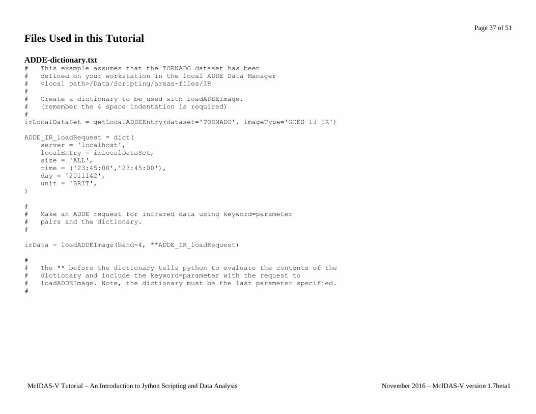
Files Used in this Tutorial ADDE-dictionary.txt # This example assumes that the TORNADO dataset has been
# defined on your workstation in the local ADDE Data Manager
# <local path>/Data/Scripting/areas-files/IR
#
# Create a dictionary to be used with loadADDEImage.
# (remember the 4 space indentation is required)
#
irLocalDataSet = getLocalADDEEntry(dataset='TORNADO', imageType='GOES-13 IR')
ADDE_IR_loadRequest = dict(
server = 'localhost',
localEntry = irLocalDataSet,
size = 'ALL',
time = ('23:45:00','23:45:00'),
day = '2011142',
unit = 'BRIT',
)
#
# Make an ADDE request for infrared data using keyword=parameter
# pairs and the dictionary.
#
irData = loadADDEImage(band=4, **ADDE_IR_loadRequest)
#
# The ** before the dictionary tells python to evaluate the contents of the
# dictionary and include the keyword=parameter with the request to
# loadADDEImage. Note, the dictionary must be the last parameter specified.
#

Page 38 of 51
McIDAS-V Tutorial – An Introduction to Jython Scripting and Data Analysis November 2016 – McIDAS-V version 1.7beta1
function.py import os
#
# Setting up a variable to specify the location of your final images
# makes your script easier to read and more portable when you share it
# with other users
#
homePath = expandpath('~')
dataPath = os.path.join(homePath, 'Data')
scriptingPath = os.path.join(dataPath, 'Scripting')
enhancementPath=os.path.join(scriptingPath, 'Color-Enhancements')
areaPath = os.path.join(scriptingPath, 'tornado-areas')
irPath = os.path.join(areaPath, 'IR')
#
# imagePath is the directory to store final images
# and/or animated gif files
#
imagePath = os.path.join(scriptingPath, 'Images')
#
# This example gets the information from the dataset created previously in the tutorial
#
irLocalDataSet = getLocalADDEEntry('TORNADO', 'GOES-13 IR')
ADDE_IR_loadRequest = dict(
debug=True,
server='localhost',
localEntry=irLocalDataSet,
size='ALL',
time=('23:45:00','23:45:00'),
day='2011142',
unit='TEMP',
)
irData = loadADDEImage(**ADDE_IR_loadRequest)
#
# assign a temperature threshold used with mask() function
#
temperatureThreshold = 250.0

Page 39 of 51
McIDAS-V Tutorial – An Introduction to Jython Scripting and Data Analysis November 2016 – McIDAS-V version 1.7beta1
#
# Applying a mask is a two part process.
# First we assign a value of 1 or missing value to a temporary data object
# Second, multiply the first results to the temporary data object
#
maskedData = mask(irData, 'lt', temperatureThreshold, 1)
finalDataSet = mul(irData, maskedData)
#
# Import enhancement table
#
IRColorTableFile = os.path.join(enhancementPath, 'Tornado-IR.xml')
IRTable = importEnhancement(IRColorTableFile)
IRTableName = IRTable.getName()
#
# Build a window and turn off the wireframe box
#
bwLines = irData['lines'] / 2
bwEles = irData['elements'] / 2
panel = buildWindow(height=bwLines, width=bwEles)
panel[0].setWireframe(False)
#
# Add layers to the existing window set enhancement table and data ranges
#
irLayer = panel[0].createLayer('Image Display', finalDataSet)
irLayer.setLayerLabel('GOES-13 Temperatures less than ' + str(temperatureThreshold) + ' %timestamp%')
irLayer.setEnhancement(IRTableName, range=(temperatureThreshold,200))
#
# Set the center latitude, longitude and scale
#
panel[0].setProjection('US>States>N-Z>Oklahoma')
panel[0].setCenter(33, -97, scale=.5)
fileName=os.path.join(imagePath, 'ir-image.gif')
panel[0].captureImage(fileName)

Page 40 of 51
McIDAS-V Tutorial – An Introduction to Jython Scripting and Data Analysis November 2016 – McIDAS-V version 1.7beta1
image-movie.py import os
#
# The ** before the dictionary tells python to evaluate the contents of the
# dictionary and include the keyword=parameter with the request to
# loadADDEImage. Note, the dictionary must be the last parameter specified.
#
# Setting up a variable to specify the location of your final images
# makes your script easier to read and more portable when you share it
# with other users
#
homePath = expandpath('~')
dataPath = os.path.join(homePath, 'Data')
scriptingPath = os.path.join(dataPath, 'Scripting')
enhancementPath = os.path.join(scriptingPath, 'Color-Enhancements')
areaPath = os.path.join(scriptingPath, 'tornado-areas')
irPath = os.path.join(areaPath, 'IR')
#
# imagePath is the directory to store final images
# and/or animated gif files
#
imagePath = os.path.join(scriptingPath, 'Images')
#
# assign a temperature threshold used with mask() function
#
temperatureThreshold = 250.0
#
# Initialize a python list
#
myLoop=[]
#
# Create a dictionary for requesting images
#
irLocalDataSet = getLocalADDEEntry(dataset='TORNADO', imageType='GOES-13 IR')
parms = dict(
server='localhost',
localEntry=irLocalDataSet,
position='ALL'
)

Page 41 of 51
McIDAS-V Tutorial – An Introduction to Jython Scripting and Data Analysis November 2016 – McIDAS-V version 1.7beta1
#
# Create a list of all available Images using listADDEImageTimes
#
dateTimeList = listADDEImageTimes(**parms)
#
# listADDEImages was successful, so now try loadADDEImage for each of the
# directories returned. There may be occasions when the loadADDEImage fails
# but we want to continue
#
for dateTime in dateTimeList:
imageTime = dateTime['time']
print dateTime['time']
ADDE_IR_loadRequest = dict(
localEntry=irLocalDataSet,
day=dateTime['day'],
time=(imageTime,imageTime),
band=4,
unit='TEMP',
size='ALL',
)
irData = loadADDEImage(**ADDE_IR_loadRequest)
#
# Applying a mask is a two part process.
# First we assign a value of 1 or missing value to a temporaary data object
# Second, multiply the first results to the temporary data object
#
maskedData = mask(irData, 'lt', temperatureThreshold, 1)
finalDataSet = mul(irData, maskedData)
myLoop.append(finalDataSet)
#
# Import enhancement table
#
IRColorTableFile=os.path.join(enhancementPath,'Tornado-IR.xml')
IRTable=importEnhancement(IRColorTableFile,overwrite=True)
IRTableName=IRTable.getName()

Page 42 of 51
McIDAS-V Tutorial – An Introduction to Jython Scripting and Data Analysis November 2016 – McIDAS-V version 1.7beta1
#
# Build a window and turn off the wireframe box
#
bwLines = irData['lines'] / 2
bwEles = irData['elements'] / 2
panel = buildWindow(height=bwLines, width=bwEles)
panel[0].setWireframe(False)
#
# Add layers to the existing window set enhancement table and data ranges
#
irLayer = panel[0].createLayer('Image Sequence Display', myLoop)
irLayer.setLayerLabel('GOES-13 Temperatures less than ' + str(temperatureThreshold) + ' %timestamp%')
irLayer.setEnhancement(IRTableName, range=(temperatureThreshold,200))
#
# Set the center latitude, longitude and scale
#
panel[0].setProjection('US>States>N-Z>Oklahoma')
panel[0].setCenter(33,-97,scale=.5)
fileName = os.path.join(imagePath, 'ir-loop.gif')
writeMovie(fileName, globalPalette=False)

Page 43 of 51
McIDAS-V Tutorial – An Introduction to Jython Scripting and Data Analysis November 2016 – McIDAS-V version 1.7beta1
image-exercise.py import os
# Setting up a variable to specify the location of your final images
# makes your script easier to read and more portable when you share it
# with other users
homePath = expandpath('~')
dataPath = os.path.join(homePath, 'Data')
scriptingPath = os.path.join(dataPath, 'Scripting')
enhancementPath = os.path.join(scriptingPath, 'Color-Enhancements')
areaPath = os.path.join(scriptingPath, 'tornado-areas')
irPath = os.path.join(areaPath, 'IR')
basePath = os.path.join(areaPath, 'BASE')
#
# imagePath is the directory to store final images
# and/or animated gif files
#
imagePath = os.path.join(scriptingPath, 'Images')
#
# assign a temperature threshold used with mask() function
#
temperatureThreshold = 250.0
#
# Create a dictionary for a basemap image
#
baseMapDataSet = makeLocalADDEEntry(dataset='TORNADO', imageType='Land Sea Mask', mask=basePath, format='McIDAS Area',
save=True)
baseMapParms = dict(
server='localhost',
localEntry=baseMapDataSet,
size='ALL'
)
baseMapData = loadADDEImage(**baseMapParms)
irLocalDataSet = getLocalADDEEntry('TORNADO', 'GOES-13 IR')
ADDE_IR_loadRequest = dict(
debug=True,
server='localhost',
localEntry=irLocalDataSet,
size='ALL',
mag=(1,1),
position='ALL',
unit='TEMP',
)

Page 44 of 51
McIDAS-V Tutorial – An Introduction to Jython Scripting and Data Analysis November 2016 – McIDAS-V version 1.7beta1
irData = loadADDEImage(**ADDE_IR_loadRequest)
#
# Initialize a python list
#
myLoop=[]
#
# Create a list of all available Images using listADDEImageTimes
#
dateTimeList = listADDEImageTimes(**ADDE_IR_loadRequest)
#
# listADDEImages was successful, so now try loadADDEImage for each of the
# directories returned. There may be occasions when the loadADDEImage fails
# but we want to continue
#
for dateTime in dateTimeList:
imageTime = dateTime['time']
print dateTime['time']
ADDE_IR_loadRequest = dict(
localEntry=irLocalDataSet,
day=dateTime['day'],
time=(imageTime,imageTime),
band=4,
unit='TEMP',
size='ALL',
)
irData = loadADDEImage(**ADDE_IR_loadRequest)
#
# Applying a mask is a two part process.
# First we assign a value of 1 or missing value to a temporary data object
# Second, multiply the first results to the temporary data object
#
maskedData = mask(irData, 'lt', temperatureThreshold, 1)
finalDataSet = mul(irData, maskedData)
myLoop.append(finalDataSet)
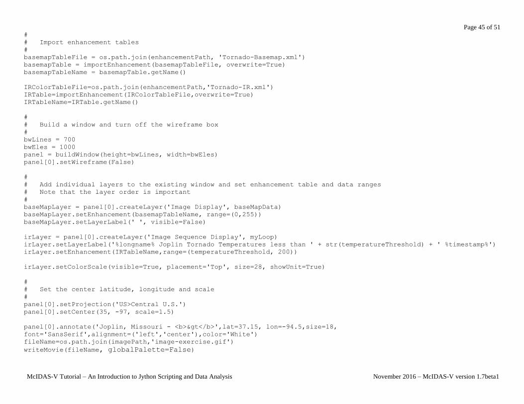
Page 45 of 51
McIDAS-V Tutorial – An Introduction to Jython Scripting and Data Analysis November 2016 – McIDAS-V version 1.7beta1
#
# Import enhancement tables
#
basemapTableFile = os.path.join(enhancementPath, 'Tornado-Basemap.xml')
basemapTable = importEnhancement(basemapTableFile, overwrite=True)
basemapTableName = basemapTable.getName()
IRColorTableFile=os.path.join(enhancementPath,'Tornado-IR.xml')
IRTable=importEnhancement(IRColorTableFile,overwrite=True)
IRTableName=IRTable.getName()
#
# Build a window and turn off the wireframe box
#
bwLines = 700
bwEles = 1000
panel = buildWindow(height=bwLines, width=bwEles)
panel[0].setWireframe(False)
#
# Add individual layers to the existing window and set enhancement table and data ranges
# Note that the layer order is important
#
baseMapLayer = panel[0].createLayer('Image Display', baseMapData)
baseMapLayer.setEnhancement(basemapTableName, range=(0,255))
baseMapLayer.setLayerLabel(' ', visible=False)
irLayer = panel[0].createLayer('Image Sequence Display', myLoop)
irLayer.setLayerLabel('%longname% Joplin Tornado Temperatures less than ' + str(temperatureThreshold) + ' %timestamp%')
irLayer.setEnhancement(IRTableName,range=(temperatureThreshold, 200))
irLayer.setColorScale(visible=True, placement='Top', size=28, showUnit=True)
#
# Set the center latitude, longitude and scale
#
panel[0].setProjection('US>Central U.S.')
panel[0].setCenter(35, -97, scale=1.5)
panel[0].annotate('Joplin, Missouri - <b>></b>',lat=37.15, lon=-94.5,size=18,
font='SansSerif',alignment=('left','center'),color='White')
fileName=os.path.join(imagePath,'image-exercise.gif')
writeMovie(fileName, globalPalette=False)

Page 46 of 51
McIDAS-V Tutorial – An Introduction to Jython Scripting and Data Analysis November 2016 – McIDAS-V version 1.7beta1
load_grid.py # import the jython library used
import os
homeDirectory=expandpath('~')
dataDirectory=os.path.join(homeDirectory,'Data','Scripting','H8')
# Add the filename to the data
band1File=os.path.join(dataDirectory,'HS_H08_20150715_0100_B01_FLDK_subset.nc')
# Initialize the loadGrid parameters.
parms = dict(
time=0,
field='albedo',
xStride = 5,
yStride = 5,
xRange = (100,200),
yRange = (100,200)
)
# load the data from the file
h8b1=loadGrid(filename=band1File,**parms)
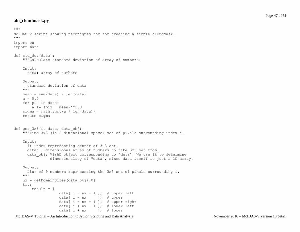
Page 47 of 51
McIDAS-V Tutorial – An Introduction to Jython Scripting and Data Analysis November 2016 – McIDAS-V version 1.7beta1
ahi_cloudmask.py
"""
McIDAS-V script showing techniques for for creating a simple cloudmask.
"""
import os
import math
def std_dev(data):
"""Calculate standard deviation of array of numbers.
Input:
data: array of numbers
Output:
standard deviation of data
"""
mean = sum(data) / len(data)
a = 0.0
for pix in data:
a += (pix - mean)**2.0
sigma = math.sqrt(a / len(data))
return sigma
def get_3x3(i, data, data_obj):
"""Find 3x3 (in 2-dimensional space) set of pixels surrounding index i.
Input:
i: index representing center of 3x3 set.
data: 1-dimensional array of numbers to take 3x3 set from.
data_obj: VisAD object corresponding to "data". We use it to determine
dimensionality of "data", since data itself is just a 1D array.
Output:
List of 9 numbers representing the 3x3 set of pixels surrounding i.
"""
nx = getDomainSizes(data_obj)[0]
try:
result = [
data[ i - nx - 1 ], # upper left
data[ i - nx ], # upper
data[ i - nx + 1 ], # upper right
data[ i + nx - 1 ], # lower left
data[ i + nx ], # lower

Page 48 of 51
McIDAS-V Tutorial – An Introduction to Jython Scripting and Data Analysis November 2016 – McIDAS-V version 1.7beta1
data[ i + nx + 1 ], # lower right
data[ i - 1 ], # left
data[ i + 1 ], # right
data[ i ], # self
]
except IndexError:
return None # can't calculate 3x3 @ boundaries
return result
def do_std_dev_test(ahi_datas):
"""The guts of the standard deviation (spatial heterogeneity) test.
We split it into a separate function because the technique is quite
different than the simple threshold tests. We loop through each pixel
instead of using array operations like "mask".
Input:
ahi_datas: dictionary with keys for each required AHI input band,
each pointing to a VisAD Data object corresponding to that
band.
Output:
VisAD Data object containing your cloudmask. 0==cloudy; 1==clear
"""
CLOUDY = 0
CLEAR = 1
# Make a data object to write the result to:
output = ahi_datas[14].clone()
# Right now we have VisAD Data objects. We need to get the actual data
# arrays before we can iterate over each pixel...
# Get the actual data array corresponding to output object:
outFloats = output.getFloats(False)[0]
# Note that changes to outFloats will change the output.
# Get the actual data arrays for each band we have data for:
ahi = dict()
for data_key in ahi_datas.keys():
ahi[data_key] = (ahi_datas[data_key].getFloats(False))[0]
# Loop through each pixel, doing any cloudy/clear checks you desire:
for i, pixel in enumerate(outFloats):
# Band 1 standard deviation test
pix3x3 = get_3x3(i, ahi[1], ahi_datas[1])

Page 49 of 51
McIDAS-V Tutorial – An Introduction to Jython Scripting and Data Analysis November 2016 – McIDAS-V version 1.7beta1
if pix3x3 is not None:
sigma = std_dev(pix3x3)
if sigma > 0.05:
outFloats[i] = CLOUDY
continue
# Band 14 standard deviation test
pix3x3 = get_3x3(i, ahi[14], ahi_datas[14])
if pix3x3 is not None:
sigma = std_dev(pix3x3)
if sigma > 5.0:
outFloats[i] = CLOUDY
continue
# passed! pixel is clear!
outFloats[i] = CLEAR
return output
def do_cloudmask(ahi_datas):
"""This is the guts of our cloudmask algorithm.
Input:
ahi_datas: dictionary with keys for each required AHI input band,
each pointing to a VisAD Data object corresponding to that
band.
Output:
VisAD Data object containing your cloudmask. 0==cloudy; 1==clear
"""
# Test number 1: Basic 11um temperature threshold check.
threshold_mask = mask(ahi_datas[14], 'gt', 220.0, False)
# Test number 2: Basic 0.47um albedo threshold check.
# From this point forward, we need to multiply by previous cloudmask.
threshold_mask = mask(ahi_datas[1], 'lt', 0.7, False)*threshold_mask
#######################################################################
# You can fill in additional clear/cloudy tests here,
# using the pattern shown in tests 1 and 2 above.
#######################################################################
return threshold_mask

Page 50 of 51
McIDAS-V Tutorial – An Introduction to Jython Scripting and Data Analysis November 2016 – McIDAS-V version 1.7beta1
def load_data():
"""Load all available input data from AHI files in 'dataDirectory'.
Returns:
Dictionary holding all the data objects read from AHI input files.
Each (integer) key corresponds to a band number, and each value is a VisAD
Data object.
"""
from glob import glob
homeDirectory = expandpath('~')
dataDirectory = os.path.join(homeDirectory,'Data','Scripting','H8')
# Filename template. We will fill in this template with actual band numbers.
template = 'HS_H08_20150715_0100_B%s_FLDK_subset.nc'
# Make a list of zero-padded strings, one for each AHI Band.
# Limit to a handful of bands for current testing: 0.47um, 6.2um, 11.2um
# See band list: http://www.data.jma.go.jp/mscweb/en/himawari89/space_segment/spsg_ahi.html
bands = ['01', '08', '14']
# Initialize the empty dictionary:
ahi_datas = dict()
# Initialize loadGrid parameters that won't change per file:
parms = dict(
time = 0,
xStride = 1, # full res
yStride = 1,
)
# Load the CMI data from each file:
for band in bands:
full_path = os.path.join(dataDirectory, (template % band))
# Get a list of actual files on disk matching our pattern for the
# current band:
files = glob(full_path)
# determine field name; it depends on whether this is IR or VIS channel.
if int(band) > 6:
field = 'brightness_temp'
else:
field = 'albedo'
if len(files) == 1:
print 'Band found: %s' % band

Page 51 of 51
McIDAS-V Tutorial – An Introduction to Jython Scripting and Data Analysis November 2016 – McIDAS-V version 1.7beta1
# Load in the data for this band:
ahi_datas[int(band)] = loadGrid(
filename = files[0],
field = field,
**parms)
elif len(files) == 0:
print 'Band not found: %s' % band
else:
raise RuntimeError("didn't find exactly one file for band %s" % band)
if len(ahi_datas.keys()) == 0:
raise RuntimeError("Didn't find any data; please check 'dataDirectory' at beginning of script.")
# Remap everything to 2km bands for 2km final output product.
for band in bands:
if int(band) > 4:
# Skip bands that are already 2km.
continue
ahi_datas[int(band)] = resampleGrid(ahi_datas[int(band)], ahi_datas[14])
return ahi_datas
def run_ahi_cloudmask():
""" The main driver function.
This is where we load data, call the algorithm, and create a display.
"""
# Load the AHI data using our custom data load function:
ahi_datas = load_data()
# Run our custom cloudmask algorithm:
cloudmask = do_cloudmask(ahi_datas)
# Get a reference to the panel we will create displays in:
panel = activeDisplay()
# Display our cloudmask and set the layer label:
cloudmask_layer = panel.createLayer('Color-Shaded Plan View', cloudmask)
cloudmask_layer.setLayerLabel(label='Custom Cloudmask. Blue=Cloudy; Red=Clear',
size=18, color='yellow')