OXFORD BUtXETlN OF ECONOMICS AND STATISTICS. 52,2 (1990)0305-9049 S3.00

MAXIMUM LIKELIHOOD ESTIMATION ANDINFERENCE ON COINTEGRATION - WITH

APPUCATIONS TO THE DEMAND FOR MONEY

Soren Johamen, Katarina Jtiselius

I. INTRODUCTION

LI. Background

Many papers have over the last few years been devoted to the estitnation andtesting of long-run relations under the heading of cointegration. Granger(1981), Granger and Weiss (1983), Engle and Granger (1987), Stock (1987),Phillips and Oullaris (1986), (1987), Johansen(1988b), (1989), JohansenandJuselius (1988), canonical analysis. Box and Tiao (1981), Velu, Wichem andReinsel (1987), Pena and Box (1987). reduced rank regression, Velu, Reinseland Wichem (1986), and Ahn and Reinsel (1987), common trends. Stockand Watson (1987), regression with integrated regressors, Phillips (1987),Phillips and Park (1986a), (1988b), (1989), as weU as under the heading test-ing for unit roots, see for instance Sims, Stock, and Watson (1986). There is aspecial issue of this BULLETIN (1986) dealing mainly with cointegration anda special issue of the Journal of Economic Dynamics and Cotitrol (1988)deeding with the same problems.

We start with a vector autoregressive model (cf. (1.1) below) and formulatethe hypothesis of cointegration as the hypothesis of reduced rank of the long-run impact matrix II = afi'. The main purpose of this paper is to demonstratethe method of maximum likelihood in connection with two examples. Theresults concern the calculation of the maximum likelihood estimators andlikelihood ratio tests in the model for cointegration under linear restrictionson the cointegration vectors 0 and weights a. These results are modificationsof die procedure ^ven in Johansen (1988b) and apply the multivariate tech-nique of partial canonical correlations, see Anderson (1984) or Tso (1981).

For ii^erence we apply the results of Johamen (1989) on the asymptoticdistribution of thelikelUuKxl ratio test. These disttibutiom are givai in termsof a multivmate Brownian motion process and are tabidated in theAppendix. Inferences on a aiyd fi imder linear restrictions can be amductedusing the usual x^ distribution as an approximation to the distribution oflikelihood ratio test. We also apply the limiting distribution of the tnaximumliketifaood estimator to a Wald test for hypotheses about a and 0.

169

170 BULLETIN

I.I The Statistical Model

Consider the model

H,:X,=n,X,_,-l-... + ntX,_,-l-^ + 4»D,+e,,(/ = l , . . . , r ) , (1.1)

where £,,...,6^ are IINp(O, A) and X_ji.n,...,Xo we fixed. Here thevariables D, are centered seasonal dummies which sum to zero over a fullyear. We assume that we have quarterly data, such that we include threedummies and a constant term. The unrestricted parameters (^, * , II,,..., n;t,A) are estimated on the basis of T observations from a vector autoregressiveprocess. For a /ndimensional process with quarterly data this gives Tpobservations and /> -I- 3p + Arp +/'(p +1 )/2 parameters.

In general, economic time series are non-stationary processes, and VAR-systems like (1.1) have usually been expressed in first differenced form.Unless the difference operator is also applied to the error process andexplicitly taken account of, differencing implies loss of information in thedata. Using A = 1 - L, where L is the lag operator, it is convenient to rewritethemodd(l.l)as

AX, = r,AX,_| + ...-l-rk_,AX,_4 + i + IIX,_t-l-/( + *D,-l-e,, (1.2)

where

r ,= - ( i - n , - . . . - n , ) , {i=i,...,k-\),

and

Notice that model (L2) is expressed as a traditional first difference VAR-model except for the term IIX,_^. It is the main purpose of this paper toinvestipte whether the coefficient matrix II contains information aboutlong-run relationships between the variables in the data vector. There arethr^ possible cases:

(i) Rank(Il)=p, i.e. the matrix II has full rank, indicating that the vectorprocess X, is stationary.

(ii) Rank(Il)=0, i.e. the matrix 11 is the null matrix Mid (1.2) corresponds toa traditional differenced vector time series modd.

(iii) 0 < rank(n) = r < p implying that there are p x r matrices o and fi such

The cointegration vectors fi have the property that fi'^, is stationary eventhough X, itself is non-stationary, in this case (1.2) esR be interpreted as anerror correction moctel, see Ett^e and Granger (19S7), Davidson (1986) orJcdiansen {1988a). Thus the main hypothesis we sttl£ consider here is thehjpotl^is of rcoint^-ati(Hi vectors

H j : n = a ^ ' , : (14)

where o and jP are p X r matrices.

INFERENCE ON COINTEGRATION 171

We further invest%ate linear hypotheses expressed in terms of the coef-ficients fi, a and fi, and in particular the relation between the constant termand the reduced rank matrix II. If D is restricted as in H^, see (1.4) and / ( # 0the non-stationary process X, has linear trends with coefficients which arefunctions of/J only through a\fi, where a^ is a/? x(j? - r) matrix of vectorschosen orthogonal to a. Thus the hypothesis /i = aP[f, or alternativelyo V /* = 0, is the hypothesis about the absence of a linear trend in the pr(x;ess.Note that when ft = a^(, we can write

where /?* = (/»', fi'o)' and Xf_t==(X;_4, 1)'. This is useful for the calculations.Since the asymptotic distributions of the test statistics and estimators dependon which assumption is maintained, it is important to choose the appropriatemodel formulation. This has been pointed out for instance by West (1989),Dolado and Jenkinson (1988). The mathematical results for the multivariatemodel (1.2) are given in Johansen (1989).

}.3. The Data

We have chosen to illustrate the procedures by data from the Danish andFinnish «;onomy on the demand for money.' The relation m=f{y,p,c)expresses money demand m as a function of real income y, price level p andthe cost of holding money c. Price homogeneity was first tested and since itwas clearly accepted by data the empirical analysis here will be for realmoney, real income and some proxies measuring the cost of holding money.Money, income and prices were measured in logarithms, since multiplicativeeffects are assumed.

The two data sets differ both as to which variables are included and thelength of the sample. More interestingly, however, the institutional relationsin the two economies have been quite different in the sample period. InDenmark, financial markets have been much less restricted tfeui in Finland,where both interest rates and prices have been subject to regulation for mostof tiie sample period. One would expect this to show up in the empiricalresults and it does.

For the Danish data the sample is 1974.1-1987.3. As a proxy for moneydemand ml was chosen because the data available on a quarterly basis arebased on more homc^eneous defimtions for ml than for ml . The cost ofholding money w ^ assiimed to be approximately measured by the differencebetween the bank deposit rate, i'', for interest bearing deposits (whidi are themain part of ml) and the bond rate, i'', which plays an important role in theDanish &xmomy. The two interest rat^ were included unrestrktedly in theaimlysis, but subsequently tested for equal coefficients with o{^K)site sipis.The inflation rate. A/?, was also inclwled as a po^ible proxy for tt^ cost of

' For a general review erf theoretical aed emprical results on the demand for money, see forinstance LakBCT(1985).

172 BULLETIN

holding money, but since it did not enter si^iificantly into the cointegrationrelation for money demand it was omitted from the present analysis.

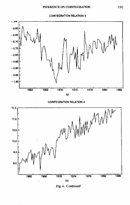
For the Finnish data the sample is 1958.1-1984.3. In this case ml waschosen since the m 1 cointegratitMi relation was found to enter the demandfor money equation more significantly and hence illustrated the methodologybetter. Since interest rates have been regulated, a good proxy for the actualcosts of holding money is difficult to find. The inflatk>n rate, Ap, is a naturalcandidate and therefore is included in the data set. Moreover, the marginalrate of interest, /'", of the Bank of Finland is included in spite of the fact thatthe marginal rate measures restrictedness of money rather than the cost ofholding money. It has, however, been chosen as a determinant of Finnishmoney demand in other studies and therefore is also included here. AU seriesare graphed in Figure 3 and Figure 4 in Section IV. The data are availablefrom the authors on request.

The p^jer is structured as follows: Section II discusses the varioushypotheses we shall investigate and in Section III the notation is introducedfor the maximum likelihood procedure. The next section derives theestimates of a and fi under-the assumption of cointegration and the last twosections investigate estimates and tests for fi and a under linear restrictions.

Throu^out, the two examples are used to motivale the statistical analysisand to illustrate the mathematically deriv^l concepts.

n. A CLASSIFICATION OF THE VARIOUS HYPOTHESES

The hypotheses we consider consists of the hypothesis Hj on the existence ofcointegrating relations combined with linear restrictions on either thecointegrating relations or their weights:

'(or j8 =

and Hf is /fy augmented by/* = o^ofor/= 2,...,5.Note that the hypothesis H,, where II is unrestridKl, can be written as Hj

with r=p. Hence, in this case the restriction /i - afi'g is the same as having /tunrestricted. When we estimate model (1.2) wider the hypothesis n = a^' thechoice of hypothesis about fi becoRKs important. Ffew the Danish data tfieredoes not seem to be any linear trend in the non-^tiooary processes (cf.Figure 3) and we will estimate modek of the form Hf. For the Finnish data,however, there seems to be a linear trend in the non-isationary processes (cf.Figure 4) and models of ttie form/f, will be ^timated.

The matrices A(p x m) and H{p x .y) are known emd define linear restric-tions <Mi the parameters a(p x r) and 0{p x r). The restrictions reduce the

INFERENCE ON COINTEGRATION 173

parameters to ^[s^r] and ^{mxr), where r&s^p and r^m^p. Theimportant distinction between the H and the H* hypotheses is that H* definea restriction on ft, namely that it lies in the space spanned by a or thata\fi = Q, hence that no trend is presaiL In the following the discussion willbe concerned with the H hypotheses, but can easily be extended to includethe case of H*. In the above scheme note that Hj = 7/4 (1H , and that H^'^H^and H4 c H2. In fact all hypotheses are special cases of H^ tf we choose eitherA or H as the identity matrix.

The relations between the various hypotheses are illustrated in Figure 1.All these hypotheses are restrictions of the matrix 11 which under H,

contains p^ parameters. Under the hypothesis H2 there are pr+{p-r)rparameters which are further restricted to sr+{p-r)r under H4. Finallymr+{s — r)r parameters remain under H5. Note also that the parameters aand p are not identified in the sense that given any choice of the matrix| ( r X r), the choice a$ and j8(§')~' will give the same matrix 11, and hencedetermine the same probability distribution for the variables. One way ofexpressing this is to say that what the data can determine is the space spannedby the columns in /3, the cointegration space, and the space spanned by a. Ingeneral we present the results normalized by the coefficient of some of thevariables, usually m 1 and ml respectively.

Note also that for each value of r{O^r:^p] there is a correspiondinghypothesis H2{r) of r or fewer cointegrating relations. The analysis makes it

Fig. 1. The relation between the various hypothesis studied, starting with the mostgeneral VAR model (//,) and introducing the restriction of cointegration {Hj) as wellas linear restricti<ms on the cointepation vectOTS (/J) and the weights (a) in / / , and

H^. The assumption of no trend fi = a^'n is indicated by a*.

174 BULLETIN

possible to conduct inferences ^ o u t the value of r by testu^ H2{r) in H^ orby testing H2( r) in H2( r -l-1).

in. THE MAXIMUM LIKELIHOOD PROCEDURE

In the following we will use die parameterization (1.2). The reason for this isthat the paratneters

( r , , . . . , r , _ j , <&,/«, n , A)

are v^ation independent and, since all the models we are interested in areexpressed as restrictions on fi and II, it is possible to maximize over all theother parameters once and for all. We shall give details in the case ofhypotheses about a and P without restrictii^ ft, but mention how results aremodified when o 'j /i = 0. Generally we use a superscript * to indicate that weare analysing a model where a'^fi = . The model with /* = 0 and 4» = 0 wasanalysed in Johansen (1988b) and Johansen and Juselius (1988).

We now consider maximum likelihood estimation of the parameters in theunrestricted model:

AX,=r,AX,_, + ...-Hr^_,Ax,_,^, + nX,_,-l-/t + * D , + e,. (3.1)

The resuhs (3.2)-(3.9) are well-known but reproduced to establish thenotation. This will be useful for discussing the estimjitors and tests later.

We first introduce the notation Zn, = AX,, Z,, denotes the stacked variablesAX,_i,...,AX,_t + ,,D,, and 1, and Z4; = X,_(t. Sinularly, F is the matrix ofparameters corresponding to Z,,, i.e. the matrix consisting of T,,..., Ti _,, ^and ft. Thus Z,, is a vector of dimeiKion p(A:-l) + 3 + l and T is a matrix ofdimension/J X (p( A: - 1 ) +3 +1).

The model expressed in these variables becomes

i-c,, (r = l , . . . , r ) . (3.2)

For a fixed value of II, maximum likelihood estimation consists of a regres-sion of Z(,, - nZn, on Z,, giving the normal equations

r T T

Z z,,,z;,=r Z z,,z',,+n Z ZJL\,. (3.3)/ - I r = l / = !

The product moment matrices are denoted:• /

M-=r" ' Z ZyZ' (j ;'=0 1 fc) (3 4)

Then (3.3) can be written as:

orMn'. 4 {3.5}

INFERENCE ON COINTEGRATION 175

This leads to the definition of the residuals

Ro,=Zo,-Mo,Mri'Z,,, (3.6)

R,, = Z,,-M,,Mfi'Zi,, (3.7)

i.e. the residuals we would obtain by regressing AX, and X,_^ onAX,_,,...,AX,_^+i,D,,andl.

The concentratai likelihood function becomes:

(3.8)

We express the estimates under the mode! //j by introducing the notation

T

s ^ = r - ' I R,,R;=M,;^-M,,M,VM,,, {i,j-o,k), (3.9)

and formulate these well-known results in

THEOREM 3.1: In the model:

//,:AX,= j j

the parameters are estimated by ordinary least squares and we have:

l i = SoAV, (3.10)

and

^~^OO~^0k^lik^k{}' (3.11)

L-^/^(H,) = |A|. (3.12)

The estimate of II inserted into (3.5) gives the estimate of T.

Under the hypothesis Hf :n = a/3' and fi = a/SJ,, which will be investigatedfor the Danish data, it is convenient to define Z , = Z,,, = AX, and let Zf, be thestacked variables AX,_|,...,AX,_4+i,D,, whereas Zt; = Xflji = (X',_ , 1).Thus we have moved the constant from the regressors into the vector Xf.^.Further, we define T* as the matrix of the relevant parameters T,,..., T _ j , ^ .Similarly we define M | and S|. Note in particular that S*i is (p +1) x (p + 1).

3.1. The Empirical Analysis ofthe Unrestricted Model Hi

Model (3.1) including a constant term and s^tsonal dummies is fitted to theDanish and Finnish money demand data described in Section 1.3. For k= 2,the residuals for the Danuh data passed the test for being uncorrelated (seeTzble 1 below). For the Finnish data, the test statistic for the residue in the

176 BUliETTN

equation for Ay is almost d^iificant. The autocorr^gram suggests that thereis some seasonality left in the residuals, but since the seasonal autocorrelationis rather small we have chosen to ignore this. Accordingly, model (3.1) withk=2 was fitted to both data sets. After conditioning on the first two datarealizations, the number of observations left for estimation was 53 in theDanish and 104 in the Finnish data.

Since the parameter estimates of Fj, * , /< and A are not of particularinterest in this paper, they are not reported. The estimates of II are reportedin Table 7 Section VI, and the standard error of regression estimates in Table1 below. The normality assumption is tested by the Jarque & Bera test(Jarque and Bera, 1980), and reported below. For the Finnish data theresiduals from the Af" and Ap equations do not pass the test. The deviationsfrom normality are mainly due to too many large residuals. They are,however, approximately symmetrically distributed around zero, whichprobably is less serious than a skewed distribution. The robustness of the MLcointegration procedure for deviations from normality has not been investi-^ted so far.

TABLE 1Some Test Statistics for the niid Assumption for the Residuals in the Model (1.2) with

k = 2

The Danish data The Finnish data

Am2

Tj 7.15r, 2.12a, 0.019

Ay

11.481.930.019

A("

10.571.060.007

Ai"

7.341.610.005

Ami

11.301.610.045

Ay

19.211.880.029

Ai'" Ap

4.30 6.9910.86 28.020.034 0.011

where r, = TX.r-i{i= 1 10)- ;

m is the number of regre^ors, 5 ^ is skewness and EK is excess kunosis.o, is the standard error of regression estimate.

IV. DERIVATION OF THE ESTIMATES OF a AND fi UNDER THEHYPOTHESIS n = o^' AND THE UKELIHOOD RATIO TEST FOR

THIS HYPOTHESIS

Consider the model Hj, where n = c^'. The estimation of r j , . . . , r t_, , *and fl is the same as before leading to (3.8). For fixed , it is easy to estimatea and A by regr^sing R,,, on /J'R, _ to <^>tain:

: (4.1)

(4.2)

INFERENCE ON COINTEGRATION 177

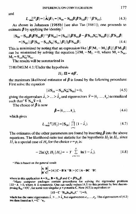
andL^^^P) = \Am = \Soo-SoJ{P'S,,fi)''fi'S,ol (4.3)

As shown in Johansen (1988b) (see also Tso (1981)), one proceeds toestimate P by applying the identity.^

,,^|. (4.4)

This is minimized by noting that an expression like | '(Mj - Mj) /31 /1 'M) |can be minimized by solving the equation | AM, -^Mj 1 = 0, where M, = S^ ,

The results will be summarized in

THEOREM 4.1: Under the hypothesis

the maximum likelihood estimator of P is found by the following procedure:First solve the equation

lAS,,-S,oSoo'SoJ=O, (4.5)

giving the eigenvalues A ,>. . .> Ap and eigenvectors F= (v,,..., v ) normalizedsuchthat^V'SttV = l.

The choice of $ is now4 = (v,,...,U (4.6)

which gives

(l-A,). (4.7)

The estimates of the other parameters are found by inserting p into the aboveequations. The likelihood ratio test statistic for the hypothesis H2 in H,, sinceH^ is a special case of H2 for the choice r=p, is:

p

, ) = - r S ln(l-A,). (4.8)i - r + l

^This is based on the general result

'A-'B| = |C | |A-BC- 'B ' |

where in this application A =S||,,, B = S^tfi and C = fi'Sttfi.'Many computer packages contain procedures for solving the eigenvalue problem

I AI - A1 =0, where A is synmietric. Ctae can easily reduce (4.5) to this problem by first decom-=CC', for some non-singutar p xp matrix C. Now (4.5) is equivalent to

jwhich has the same eigenvalues A j >.. . > i^ but eigenvectors e, c . The eigenvectors of (4.5)are then found as v, = C'" 'e,.

178 BULLETIN

Similarly the likelihood ratio test statistic for testing Hjlr) in Hjir +1) isgiven by

|r+l)=-rin(l-i,,,). (4.9)

Under the hypothesis Hf.Il^afi' and fi = afi'o the same results hold butderived from S | rather than S,y.

The asymptotic distributions of the likelihood ratio test statistics (4.8) and(4.9) are found in Johansen (1989), and are not given by the usual x' distribu-tions, but as multivariate versions of the Dickey-Fuller distribution. Thesedistributions are conveniently described by certain stochastic integrals, andcan be tabulated by simulation, see the Appendix.

Consider first the case a\fi~Q.By suitably normalizing the equation (4.5)and letting F— =» one can show that r(A^+,,..., Ap) converge to the roots ofthe equation

?'dr- F(dU')Jo Jii

¥F'dt-\ F(dU') (dU)F' = 0, (4.10)

where U(f) ={[/,(/),..., (7p_,(f)| is a (p-r)-dimensional Brownian motionand the (p—r)-dimensional stochastic process F(/)={F|(/'),...,f^j_^(/)} isdefined by

Ui{s)ds, (i = l, . . . , /?-r). (4.11)

Further FF'dr 'is a(p-r)x(p-r) matrix of random variables defined byJo

the ordinary Riemarm integrals

FMFj(t)dt, (/,; = !,. . . ,p-r), (4.12)

and

i><^''-[rF(dU')= I (dU)F'

is define as the matrix of stochastic integrals*

' i

(t,/ = l,. . . ,p-r). (4.13)

INFERENCE ON COiNTEGRATiON 179

With this notation it follows tiiat the statistk (4.8) satisfies

-2ln{Q;H2\Hi)=-T i m-A,)= I rl-

which converges weakly to

- f r (dU)F' FF'dr F(dUU

where tr{M] denotes the trace of the matrix M. The statistic (4.8) is thereforecalled the trace statistic (trace). Similarly

converges weakly to

(dU)F'l I FF'drl I F(dU')[,u LJu J J "

where A,, {M} denotes the marginal eigenvalue of the matrix M. The statistic(4.9) is called the maximal eigenvalue statistic (A^ ).

lfr=p-l, then both U and F are one dimensional. Then the test statisticsare equal, since the trace equals the (maximal) eigenvalue, and the asymptoticdistribution of the statistic can be expressed as

[U-U]dU\ / [U{s)-UfdsLJn j / Ju

where

U= U{u)du.Jo

This statistic is the square of the statistic f tabulated in Fuller (1976) p. 373.The distribution of the trace and the maximal eigenvalue of the roots of

(4.10) depend only on the dimension p-r, i.e. the number of non-stationary

••The definition of a stochastic integral is analogous to the definition of a Riemann integral.We let U and F be two continuous stochastic processes on the unit interval like the Brownianmotions. Then we consider a partion of the unit interval and the Riemann sum

The function U( •) has infinite variation but finite quadratic variation, i.e,sup{f^)Zjt(t/(Ji)- t/((t_,))^^c< « . This can be used to prove the existence of the linwt of R in^2. i-e- there exists a nuidom variable, which we shall call jFdU, such that E{R-\FAUfconverges to zera

180 BULLETIN

components under the hypothesis. The distributions are tabulated by simula-tion and are given in the Appendix in Table A2.

Next consider the case where a'^/t # 0, i.e. the trend is present under thenull hypothesis. We can express the results in this case by choosing a differentdefinition of F:

- U,{s)ds,

{i=p-r).

(4.14)

(4.15)

It is instructive to consider again the case of p~r=l, where the statisticreduces to

which is distributed as ;(^(1). This is the well-known result (West (1989)) thatif the linear trend is present under the hypothesis of non-stationarity then theusual asymptotics hold for the likelihood ratio test. The distribution of thetrace and maximal eigenvalue of the equation (4.10) with this choice of F istabulated by simulation in the Appendix and given in Table Al.

Since the distribution with a\fi = Q has broader tails, cf. Tables Al andA2 in the Appendix, the p-value should be calculated from the latter distribu-tion.

Under H^ (i.e. ft = a^f,) the asymptotic distribution of the test statistics(4.8) and (4.9) can be shown to be distributed as above but with F defined by:

These distributions are tabulated by simulation in Table A3. The relationbetween the applications of the three distributions is illustrated in Figure 2below:

F=U-0

T* = irl J d unjPF' du] '

H,

Fig. 2. The relation betweMi the hypotheses H^, H^sad if?, and the test statisticsused to test them. Note that 7"? = Tz + U{ \yu{\).

INFERENCE ON COINfTEGRATION 181

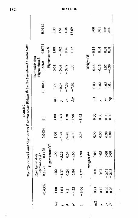
4.1. The Empirical Analysis^

ln Table 2 the estimated eigenvalues A, the normalized eigenvectors ^, andweights W=Sfl^^ are reported, for the two data sets. The graphs correspond-ing to the eigenvectors and the original data are presented in Figures 3 and 4.Note that the eigenvectors v* for the Danish data are of dimension 5, wherethe last coefficient is the estimated intercept. For the Finnish data fi isassumed to contain effects both from the intercept and from the linear trend(see discussion in Section I).

In Table 3 the likelihood ratio test statistics are calculated and comparedto the 95 percent quantiles of the appropriate limiting distribution. Twoversions of the test procedure are reported in Table 3. The first is based onthe trace and the second on the maximum eigenvalue, see Theorem 4.1, (4.8)and (4.9).

The Danish DataOn the basis of the plots of the series (see Figure 3) a model without a lineartrend in the non-stationary part of the process was assumed. Thus a constant1 was appended to the vector X,_2, and the calculations were performed asdescribed in Section I, giving the matrices S|. The results of the eigenvalueand eigenvector calculations are given in Table 2. First we consider thenumber of cointegration vectors, beginning with the hypothesis r<. 1 versusthe general alternative /f,. Using the trace test procedure gives-2hi(Q)=-rSt=2hi(l-A*)= 19.06.

The 95 percent quantile, 35.07, in the asymptotic distribution, see TableA3, is not significant. Hence there is no evidence in the Danish data for morethan one cointegration relation. If we test the hypothesis that r= 0 in /f, weget a test value of 49.14, which is found to have a /»-value of appr. 10 percent.If instead we apply the maximum eigenvjdue test, and test H,(r=O) inH2( r^ 1) we find - 2 ln( <2; r=01 r^ 1) = 30.08 which is in the upper tail of thedistribution of A,^ for r= 0 with a /?-value of 2.5 percent. We conclude thatthere is only one cointegration vector in the Danish data. This hypothesis willbe maintained below. It must be noted that since the TA, are ordered theycannot be indqjendent, not even in the limit.

Thus all the tests performed in Table 3 are highly dependent on oneanother.

Finally, as a check that the maintained assumption about the absence oftrend is data consistent, the test for Hf(r^ 1) in //^(r^ 1) (see Figure 2) wasperformed:

( -2

calculations have ^xea perfcsmed in the computer package RATS, VAR Econo-metrics, Inc/Doan Associates.

182 BULliTlN

pd

o o op,.., , ^ ,-H m

a

I

fO

pd

3 ^

p

Ie.S2 aS e

d oI I

^ ^ O Op p P Pd d d -^

-4 p p pd d d d

I I

^ fO t* O•^ —• p rod d — d

I I I

d

O 00 ^p !3\ p-4 d t-

I I

ro rsi in —Hp p p pd d d o

aJ •«

p-4 d ^ —<

I 1

p00I

opd

o o op p pd d d

o

I o » o op 00 •'t ro

o o o op p p pd d d d

.1

oZocCO

1

ro (N 00~:, d -^i

o Tf m O Op p p pd d d d

O Cvl —H COp p p pd d d o

I I

ro r-p r1

H (N

1

VOpSO

1

(M <N| r o•PH p p

d d d

INFERENCE ON COINTEGRATION 183TABLE 3

Test statistics for the hypothesis H*, and H^for various values ofr versus r+I (k ^J andversus the general alternative H, (trace) for the Danish and Finnish data. The 95%

quantiles are taicen from Table A 2 (H2) and A3 (Hy

r<3r^lr<.\r=0

The Danish data

trace

2.358.69

19.0649,14

trace(0.95)

9.0920,1735.0753.35

Amax

2.356.34

10.3730.08

(0.95)

9.0915,7521.8928.17

r<3r^2r< l/-=0

The Finnish data

trace

3.1111.0137,6576.14

trace(0.95)

8.0817.8431.2648.42

• " •mas

3.117.90

26.6438.49

''•max

(0.95)

8-0814-6021,2827.34

thusThis relation holds, since |Soo|nt(l-A;)=|S^(,|nf(l-ASn^S^ 'Sio|. The asymptotic distribution of the test statistic is xH^not significant.

The coefficient estimates of the cointegrating relation are found in Table 2as the first cdumn in V*. The interpretation of the cointegration vector as anerror correction mechanism measuring the excess demand for money isstraightforward, with the estimate of the equilibrium relation given by

.22''+6.06.

Similarly d is foimd as the first column in the matrix W* = So2^*:

d' = (-0.213,0.115,0.023,0.029).

The coefficients of d can be interpreted as the weights with which excessdemand for money enters the four equations of our system, and it is natural togive them an economic meaning in terms of the average speed of adjustmenttowards the estimated equilibrium state, such that a low coefficient indicatesslow adjustment and a high coefficient indicates rapid adjustment. In the firstequation, which measures the changes in money balances, the average speedof adjustment is approximately 0.213, whereas in the remaining threeequations the adjustment coefficients are lower though of the 'correct' sign. Inparticular the last two adjustment coefficients are low, and the hypothesis thatsome subset of the adjustment coefficients is zero will be formally tested inSection VI.

The Finnish DataAs discussed earlier a model that allows for linear trends is fitted to theFinnish data. The estimated eigenvalues, vectors and weights are given inTable 2 and the test statistics in Table 3, which indicate that at least 2 butpossibly 3 cointegration vectors are present.

The acceptance of the third relies on a p-vaiue of approximately 20percent, which usuaUy would be considered too high. But since the power of

184 BULLETIN

REAt MONEY STOCK IN DENMARK

7.50

7.40 -

7.30 -

7.20 -

7.10 -

7.00

1976 1978 1980 1982 1984 1986 1988

REAL INCOME IN DENMARK

1976 19TO T ^ 1^2 1984

(b)

Fig. 3. The graphs of the cointegration relation V|X, lor j= 1,4 and the or^nalDanish data. The sample is: 1974.1-rl987.3.

INFERENCE ON COINTEGRATION 185

BOND RATE IN DENMARK

1976 1978 1980 1982 1984

(c)

DEPOSrr RATE IN DENMARK

1976 1978 1986 1988

Fig. 3. Continued

186 BULI.ETIN

COINTEGRATION RELATION 1

1976 1978 1980 1982 1988

COINTEGRATION RELATION 2

0.150

1976 1978 1^0 1982 1984 19S6

(f)

Fig. 3. Continued

1988

INFERENCE ON COINTEGRATION 187

COINTEGRATION RELATION 3

1976 1978 1980 1982 1984 1986 1988

(g)

COINTEGRATION RELATION 4

1.00

1.30

-0.20 -

1976 1978 1980 1982 1984 1986 1988

F%. 3. Continued

188 BULLETIN

REAL MONEY STOCK IN FINLAND

4.00

3.80 -

3.60 -

3.40 -

3.20 -

3.00 -

1962 1966 1970 1974 1978 1982 1986

(a)

REAL INCOME IN FINLAND

5.00

4.20 -

4.00 -

Fig.4. The graphs of the cointegration relation VjX, for i = l , 4 and the originalFinnish data. The sample is: 1958.1-1984.3.

INFERENCE ON COINTEGRATION 189

MARGINAL INTEREST RATE IN FINLAND

0.310

0.260 -

0.210 -

0.160

0.110

1962 1966 1970 1974 1978 1982 1986

(c)

INFLATION RATE IN FINLAND

0.0600

0.0500 -

0.0400 -

0.0300 -

0.0200 -

0.0100 •

1962 1966 1970 1974 1978 1982 1986

Id)

Fig. 4. Continued

190

-1 .00

-1.50 -

-2.00

-2.50 -

-3.00 -

1962

BULJLETIN

COINTEGRATION RELATION 1

1966 1970 1974 1978 1982 1986

le)

COINTEGRATION RELATION 2

1966 1970 1974 1978 1982 1986

(f)

Fig. 4. Continued

11.5

11.0 -

10.5 -

10.0 -

1962

INFERENCE ON COINTEGRATION

COINTEGRATtON RELATION 3

191

1966 1970 1974 1978 1982 1986

COINTEGRATION REtj^TlON 4

1962 1966 1970 1974

(h)

Fig. 4. Continued

1978 1982 1986

192 BULLETIN

the tests are likely to be low for cointegration vectors with roots close to butoutside the unit circle, it seems reasonable in certain cases to follow a testprocedure which rejects for higher p-values than the usual 5 percent. Onereason why we have kept r= 3 in this case is that the hypothesis of propor-tionality between money and income, i.e. jS,, = -^ ,2 seems consistent withthe data for the 3 eigenvectors.* If m 1 and y appear in a cointegration vectorwith equal coefficients of opposite sign, they should do so in all cointegrationvectors, see Section V.

Next we test the hypothesis that the linear trend is absent, i.e. Hf(3) inl 3). We found that

|S*,

Since the asymptotic distribution of this statistic is x (l)> it is significant, andthe hypothesis i/ji^) is maintained. We find ^ as the first three columns of ^from liable 2 and d as the corresponding columns of the weights W. Notethat given the full matrices V and VV one can estimate a and P for any valueofr.

For the case r>\, the interpretation of P and d is not straightforward. Aheuristic interpretation is however possible by considering the estimates inTable 2. Note that 0i,2'°-$u> '^, 1'2>3, and that 02 is approximatelyproportional to (0,0,0,1). I'hus, $^,$2 ^nd ^3 can be approximatelyrepresented as linear combinations of the vectors ( - 1,1,0,0), (0,0,0,1), and(0,0,1,0), implying that ml-y, i"" and Ap are stationary. This means that theonly interesting cointegration relation found is between m 1 and y. However,a linear combination between these three vectors might be more stable (interms of the roots of the characteristic polynomial) than the individualvectors themselves and this linear combination could in fact be theeconomically interesting relation. In particular, one would expect that the lin-ear combination, which is most correlated with the stationary part of themodel, namely the first eigenvector, is of special interest. Although there issome arbitrariness in the case r > 1, the ordering of tfie e^envectors providedby the estimation procedure is likely to be useful.

The estimates reported in Table 2 indicate diat $2 is approximatelymeasuring the inflation rate, whereas $i and ^3 seem to contain informationabout ml-y. Note also that d,i and d^j have opposite sign. The sign to beexpected for 'excess demand for money' sho^d be negative, but di3dominates ctn, so that the 'excess demand for moliey' enters with a negativesign in the first equation. The value of dj2 can be interpreted as the w e ^ twith which the inflation rate enters equation i. M Table 7 Section VI, the

' It seems reasonable to denote the first coordinate of the cointegraticm vector fii, say, by fin.In ordinary matrix notation we then have fi^i - fi^j.

INFERENCE ON COINTEGRATION 193

estimate of II = o^', i.e. the estimate of the combined effects of all threecointegration vectors, is reported. It is striking how well the proportionalityhypothesis between money and income is maintained in all equations of thesystem.

This completes the investigation of the model /fj ^^^ ^* in H^ and wetum now to the models H^ and Hf in / / j .

V. ESTIMATION AND TESTING UNDER LINEAR RESTRICTIONS ON P

Mode] 7/3 :/fl = Hflj is a formulation of a linear restriction on the cointegrationvectors. The hypothesis spiecifies the same restriction on all the cointegrationvectors. The reason for this is the following: If we have two cointegrationvectors in which m and y, say, enter then any linear combination of theserelations will also be a cointegrating relation. Thus it will in general be poss-ible to find some relation which has, say, equal coefficients with opposite signto m and y, corresponding to a long-run unit elasticity. This is clearly notinteresting, and only if the proportionality restriction is present in all ySvectors, is it meaningful to say that we have found a imit elasticity.

5. /. Likelihood Ratio Tests

Under H3 we have the restriction ^ = H9 where H is (p x j), but that meansthat the estimation of ri,...,rjt_j, 4>, /i, a and A is given as for fixedjS = Hqj, and q> has to be chosen to minimize

I qp'(H'S«H-H'S,oSoo'So,H) flP|/| q>'{n'S,,U) q>\ (5.1)

over the set of al! 5 x r matrices ^. This problem has the same kind ofsolution as above and we formulate the results in Theorem 5.1 below. Asubscript indicates which hypothesis we are currently working with.Throughout, the estimator witiiout subscript will be the estimator under //,o r H t

THEOREM 5.1: Under the hypothesis

we find the maximum likelihood estimator of j3 as follows: First solve

I AH'S^H - H'S^oSo-o'So;tH | = 0, (5.2)

for i j I >. . .>i3^ and V3 = (v3i,...,¥3.,) normalized by V3(H'SkjH)V3 = I.Choose

* = (*3.,,-,*3.,)and43 = H*, (5.3)and find the estimates of a, A and T fi-om (4.1), (4.2), and (3.5). Themaximized likelihood bwomes

194 BULLETIN

which gives the likelihood ratio test of the hypothesis Hj in H2 as

i,Ml - i l- (5.5)The asymptotic distribution of this statistic is shown in Johansen {1989) to beX^ with r{p—s) degrees of freedom.

Under the hypothesis H*:fi=Hq> and fi = afi'^, the same results hold.

5.1.1. The Empirical Analysis

The Finnish DataWe consider the hypothesis that there is proportionality between money andincome, so that the coefficients of money and income are equal with oppositesign, i.e.

H,:^,,= -^,,2, (/= 1,2,3)

In matrix notation the hypothesis can be formulated as:

/ -

\

1100

0010

0001

where ^ is a 3 x 3 matrix. Solving (5.2) gives the eigenvalues in Table 4.These are compared to the eigenvalues of the unrestricted model H2. Thetest statistic is calculated as -21n(2) = 0.02 + 3.51+ 0.29 = 3.82 which iscompared to ;u^95(r(/7-s))=;t;^(3(4 —3)) = 7.81. ThiK the hypothesis ofequal coefficients with opposite sign for m 1 and y, is clearly accepted. Thecorresponding restricted ^-estimates hardly change at all compared to theunrestricted estimates of Table 2 and they are therefore not reported here.

With the imposed proportionality restriction we now have three cointegra-tion vectors restricted to a three dimensional space defined by the restrictionthat m 1 and y have equal coefficients with opj)osite sign. Thus the hypothesisif3 is really the hypothesis of a complete specification of sp{p). In this spacewe can choose to present the results in any basis we want and it seems naturalto consider the three variables ml—y, i"' and Ap, Thus the conclusion aboutthe Finnish data is that the last two variables C" and Ap are alreadystationary, and the first two, y and m 1, are cointegrated.

The Danish DataIn the Danish data we found r= 1. Based on the imrestricted estimates in theprevious section it seems natural to formulate tveo linear hypotheses in thiscase, both of which are economically meaningful:

INFERENCE ON COINTEGRATION 195

and

In matrix formulation the first hypothesis is expressed as

1 0 0 0- 1 0 0 0

0 1 0 00 0 1 0

L 0 0 0 l j

where qj is a 4 x 1 vector. Solving (5.2) gives the eigenvalues in Table 4.These are compared to the eigenvalues of the unrestricted H^ model.

The test of //f, in //f consists of comparing Af j and A!f by the test

The asymptotic distribution of this quantity is given by the ;f distributionwith degrees of freedom r{p-s)= 1(4-3)= 1. The test statistic is clearly notsignificant, and we can thus accept the hypothesis that for the Danish data thecoefficients of m2 and y are equal with opposite sign.

The second hypothesis that the coefficients for the bond rate and thedeposit rate are equal with opposite sign is now tested. This hypothesisimplies that the cost of holding money can be measured as the differencebetween the bond yield and the yield ftom holding money in bank deposits.Since H^, was strongly supported by the data, we will test //J2 within //f,.This will now be formulated in matrix notation as

" 1- 1

000

001

- 10

00001

where y is a 3 x 1 vector. Solving (5.2) we get the eigenvalues reported inTable A. The test for the hypothesis is given by

which should be compared with the x^ quantiles with r\s^ -52)= 1(4-3)= 1degree of freedom. It is not significant and we conclude the analysis of thecointegration vectors for the Danish demand for money by the restrictedestimate

iJ ' = ( 1.00, -1.00,5.88, -5.88, -6.21),

The corresfKMiding estimate of a is given by

a* = (-0.177,0.095,0.023,0.032).

196 BUUBTIN

TABLE 4The Eigenvalues and the Corresponding Test Statistics for Testing Restrictions on fi

The Finnish dataEigenvalues A, - 7" ln( 1 - A,)

',: 0.309 0.226 0.073 0.030 38.49 26.64 7.89 3.11',: 0.309 0.199 0.070 38.47 23.13 7.60

The Danish dataEigenvalues Af —7"ln(l-Af)

'f. 0.433 0.178 0.113 0.043 0 30.09 10.36 6.34 2.35 0't,: 0.433 0.172 0.044 0.006 30.04 10.01 2.36 0.32'?,: 0.423 0.045 0.006 29.16 2.44 0.32

5.2. The Wald Test

Instead of the likelihood ratio tests which require estimation under the modelH2 and 7/3, one can directly apply the results of model H2 given in Table 2 tocalculate some Wald tests. The idea is to exprras the restrictions on j8 asK'p=O and then normalize K'/? by its 'standard deviation'.

It is shown m Johansen (1989) that if v* denotes the eigenvectors cor-responding to A5,..., A , (see the Danish data in Table 5) then, in case r= 1,the quantity

r'-i) z1/2

is asymptotically Gaussian with mean 0 and variance 1. Hence K* = (K', 0)',such that K*'fi* = K'/3, i.e. the contrast involves oaiy the coefficients of thevariables, not the constant term. This statistic is easily calculated fromTable 5.

If more than one cointegration vector is present, as in the Finnish data,then the Wald statistic is gjven by

where v is the eigenvector corresponding to A4, aad 6 = diag(Ai, Aj, ^3) (seethe Finnish data in Table 5). The asymptotic distribution of this statistic is x^with tip-s) degrees of freedom, where K fc p'x.{p-s}. In this caser=p-l = 3, and since r^s^p = 4 and, since s»p is no restriction, we canonly test a hypothesis with s = r=p —1-3, coiresponding to a completelyspecified fi.

The above test statistics require the nonnaUza^n of fi and v as in (4.5). Analternative expression for this statistic which can be ^^lied for anynormalization is

INFERENCE ON COINTEGRATION 197

5.2.1. The Empirical AnalysisSince the calctilations are numerically simpler for the normalizationVStiV = I, it will be tised to illustrate the Wald tests. In Table 5 the eigen-values and eigenvectors for this normalization Eire reported.

7?ie Danish DataWe start by the hypothesis

expressed as K'p = {1,1,0,0) P = 0. The Wald statistic is then calculated asfoUows:

First, T^I^K'p = 53^l\ -21.97 + 22.70) = 5.31, and

5

I (K*'v*)2 = ( 14.66-20.05)2+ (7.95-25.64)2

Then the test statistic becomes

w = 5.31/(1/0.4332-l)x 360.13)'/-= 0.24.

The second hypothesis

is tested in a similar way. Note however, that //f 2 is now tested within Hf andnot within /ff,. The test statistics becomes 1.32. Both these statistics areasymptotically normalized Gaussian and the values found are hence notsignificant.

The Finnish DataFor the Finnish data we only test the hypothesis:

^ 3 : ^ . 1 = - / 3 , 2 , (i = 1,2,3).

This can be formulated as K'y? = (1,1,0,0) P = 0.First we find from Table 5 that K'w'K=(1.38 + 2.22)^ = 12.96 and

^(-11.13 + 10.24)-^^_^3."'0.0731" - 1

The test statistic becomes w^= 104x0.83/12.96 = 5.66, which is notsipifiramt in the ;f distrilwtion with 3 degrees of freedom.

Notice that the Wald test in aO cases givra a value of the test statistic whichis lar^r tijan the value for the likelihood ratio test statistic. This just

198 BUU£TIN

(S

qd

O * ^ H ts ^. d 2 - : d <s

o —' -^ I

1:J3

.2? 00

Ocs

iO f^ (^

p rs --\O ON •<:t'I I 2

»O) 00ts ts

Id

I

O "-

d

tsI

oot s -H

I

tsI

.1 •S"3td >Q g

v ^ 00 00OS VO t s 00

1

H " U|d •<t d-H ts

I

r~ o ts >»•

-^ ts -cj-' fsfN) ( ^ • ^^ : H^K

INFERENCE ON COINTEGRATiON 199

emphasizes the feet that we are relying on asymptotic results and a carefulstudy of the small sample properties is needed.

VI. ESTIMATION AND TESTING UNDER RESTRICTIONS ON a

Let US now turn to the hypothesis H4 where a is restricted by o = A V in themodel H2. Here A is a (pxm) matrix. It is convenient to introduceB{px{p-m)) = Ai, such that B'A = O. Then the hypothesis H^, can beexpressed as B'a = 0.

The concentrated likelihood function (3.8) can be expressed in the var-iables given by

A'(Ro, - a/J'R,,) = A'Ro, - A'A V^'R^, (6.1)

(6.2)

In the following, we factor out that part of the likelihood function whichdepends on B'Rg,, since it does not contain the parameters V and fi. To savenotation, we define:

A^=A'AA, A^j = A'AB, S^^^ = S„ - S S ft'S i

= A'So, - A'SooB(B'SooB)- 'B'So*, etc.

The factor corresponding to the marginal distribution of B'R , is given by

- Z (B'Ro,)'A^,HB'Ro,)/2L (6.3)

and gives the estimate

A,, = S,, = B'SooB, (6.4)

and the maximized likelihood function from the marginal distribution

(6.5)

The other factor corresponds to the conditional distribution of A'R , and Rj,conditional on B'RQ, and is given by

X A-',(A'Ro, - A'A#'R,, - A«,A,VB'Ro,)/2 j . (6.6)

It is a well-known result from the Aeoiy of the midtivariate normal distribu-tion that the parameters Aji, , A^A^^^ Mid A^^^ are variation independentand hence that the esdtnate of A j A ' is found by regression for fixed ^ and

200 BULUETIN

/3 givingKJ^-M'( V, ;»)=(S,, - A'AVJS'S,,) S^,', (6.7)

and new residuals defined by

In terms of ft^ and ft^ the concentrated likelihood function has the form (3.8)which means that the estimatiOTi of /J follows as before.*

THEOREM 6.1: Under the hypothesis

the maximum likelihood estimator of fi is found as follows: First solve theequation

|AS,,.,-St,.,S;^',S«,.,| = O, (6.8)

giving i^.i >...> A4.«>i4^.,, = ... = i4.p = 0 and^4 = (V4,,...,V4,,) normalizedsuchthatSi' S^ti (, 4 = 1.

Now take

k = {Kl Kr\ (6-9)which gives the estimates

^=(A'A)- 'S,, .^4 (6-10)and

oB(B'SooB)-iB'So,)44, (6.11),«.* ,,.^ = S^,,,-A'd4d;A, (6.12)

and the maximized likelihood function

"' (6.13)

The estimate of A can be foimd from (6.4), (6.7) and (6.12), and T isestimated from (3.5).

The likelihood ratio test statisic of H^ in / / , is

- 2 hi(Q; H41 Hj) = r I ln!( 1 - k,M 1 - A,)}. (6.14)1 - 1

The asymptotic distribution of this test statistic is pven by a x^ distributionwiA r{p-m) degrees of freedom, see Johansiai (1989). The same resultholds for testing HJ: a = A^ in /f f.

^It is convenient to calctdate the rdevant product momem matrices as

INFERENCE ON COINTEGRATION 201

The following very simple CoroUmy is usefiil for explaining the role ofsingle uation analysis:

COROLLARY 6.2: If m = r = 1 then the maximum likelihood estimate of fi isfound as the coefficients of X,_^ in the regression of A'AX, on X,_j, B'AX,,and AX, _ 1,..., AX, _ ;t +1, D, and the constant.

PROOF: It suffices to notice that when m = r = 1, then only one cointegra-tion vector has to estimated. It is seen from (6.8) that since the matrixSna./rSaa'aSat ft is singular and in feet of rank 1, then only one eigenvalue isnon-zero, and the corresponding eigenvector is proportional to SZk,t^ka.b->which is exactly the regression coefficient of R , obtained by regressing A'R ,,on B'Rfl, and R^. This can of course be seen directly from (6.6) since A'A^ is1x1 and can be absorbed into fi, which shows that fi is given by the regres-sion as described. If, in particular, a is proportional to (1,0,...,0), thenordinary least squares analysis of the first equation will give the maximumlikelihood estimation for the cointegration vector. An empirical illustration ofthis will be presented below.

Finally we just state briefly how one solves the estimation and testing of themodel H^.fi = Yl<p and a=Aq). In this case we note that ^'R^, = ^'H'R^,which leads to solving (5.2) where R , has been replaced by H'R^,. Thusrestricting fi to lie in 5p(H) implies that the levels of the process should betransformed by H'.

Since a = A V we solve (6.8), where we have conditioned on B'R ,. ln otherwords if we assume that the equations for B'R , do not contain the parametero, i.e. B'a = 0, then we can correct for these before solving the eigenvalueproblem. It is now clear how one should solve the model H^=H^PiH^,where restrictions have been imposed onfias well as on a, namely by solvingthe eigenvalue problem

i AH'S,,.,H -H'S^. ,S; , : ,S^ ,H I = 0. (6.15)

This gives the final solution to the estimation problem of H^. Notice how(6.15) contains the previous problems by choosing either H = I or A=I orboth. We have, however, chosen to present the analysis of restrictions on fiand a separately in order to simplify the notation.

Finally, note that a linear restriction on fi implies a transformation of theprocess, and that a linear restriction on a implies a conditioning. Thus all thecalculations can easily be performed starting with the product momentmatrices Sy and applying the usual operations of finding marginal (trans-formed) and condidonkl variances followed by an eigenvalue routine.

6.1. The Empirical Analysis

In SectiOTi V it was shown that the hs^thesis about proportionality betweenmoney and income, /3, i = -fii2, was accepted both for the Danish and tiieFinnish data, and that the hypothesis ;3|3= - ^ , 4 was accepted for theD k h data. Thus it seems natural to move directly to the H^ and the H^

202 BULLETIN

hypothesis, see Section n, and test hypotheses about a in the /^-restrictedmodels. For illustrative purposes we will, however, also present the empiricalresults for just one H^ hypothesis, i.e. a restriction on o for unrestricted fi.

The Danish DataWe denote the cointegration vector by {fi^,...,fi^) and the weights by(a,,...,0:4). Since we have no a priori hypothesis about the a's except thata, ?* 0, we have at most three hypotheses about zero restrictions on a to test.We have chosen to demonstrate the hypothesis: H^^: 03 = 0, in the text, andreport the results of other tests in Table 6.

The test results are sununarized in the upper part of the table. Theestimates of fi^ and a^ are presented below the test statistics. To facilitatecompar^n with the previous results the first column of the table gives theestimates under the unrestricted model /ff, the second and third under oneand two fi restrictions, the next three under three o restrictions and finallythe last column gives the estimates under three o restrictiors but forunrestricted fi.

Based on the calculated values of — T ln(l —A* j) in Table 6 it is nowpossible to test any of the three a hypotheses H*;, i= 1,2,3 against H%2, orany of the //f, hypotheses with fewer restrictions on a. The likelihood ratiotest statistic for H*, versus H*j is calculated as

which is asymptotically distributed as ;i; with {p-{p-i))r = i degrees offreedom, when r = 1. For instance we consider / / | , ve3 sus H%2 and find

The other tests have been linearly ordered in Tj4)le 6, and we can choose anyhypothesis of interest and test against hypotheses with fewer restrictions.Since we had no stroi^ a priori hypotheses abcwt a j , a^ and 04, the varioust^ts we have performed can be seen as a form for data exploration ratherthan as specffication testing in the strict sense.

We proceed to the H* hypotheses described in die last column of Table 6,

^4,1: «2 = a J = 04=0

for unrestricted fi. As shown in Corollary ^2, the acceptance of thishypothesis would legitimize the use of single ^^aation estimation of a and fiand is therefore of particular interest.

The hypothesis HX,i is first tested by the fikelihood ratio test and thecorrespondii^ estimates of a and ^ dmved. Ws dien give tlie correspondingordin£U7 least squares estimates iuul show that the two procedui^s give thes^oe result.

INFERENCE ON COINTEGRATION 203

IO

•g

s

SI

1*1

II

I

I ti

^ «

•=0.I

I I

I2

tn tsen rfd en

ts

VO00 -H

ts o\

en rnd tn

tstn •*•*. Pd dm

men Ov•^_ od d

en

—1 O •* c sI I

O O 00 oo rtO O 00 00 rj

I I

O 00 00 r~i

I I I

O O >o m tsp p Ov O; r-j^H T H W^ U^ VO

I I I

tsd o o o

o o o o

o o o o

ts O\ O\<n OS tsr.H p pd d o dI

t— u~> en t soooooo^H r^oststnp p o q o q t s - ^ p p pT.Hrt>ri>r!v6 d d d d

I I I I

ts 00 (N| OO O O ^ ^ - O ts enppentsts_ ts-^ppF-H ^-4 V^ "^ VO O O O O

I I I I

oen^tsvo rtrttstso o ts rs o ts -H p pd d d d

204 BULLETIN

The appropriate A and B matrices are now

/O 00'0

on the basis of which the matrices SJ j , , S%, j , , S* j , and S* j, can becalculated. Solving the eigenvalue problem (6.8) gives one eigenvalue 0.357and consequently one eigenvector 0, as well as one estimate d. Normalizedby the coefficient of m 2 the estimates are

, -0.96,4.76, -2.57, -6.58)

) = (-0.25,0,0,0).

The test statistic for this hypothesis about a is then given by

- 2 In(G; / / t i I //J) = r{in( 1 - i t , ) - hi(l - if)}

= 30.09-23.42 = 7.67 < 7.81

Although the test statistic is not significant at the 5 percent level it would beso at a slightly higher level. On the basis of this we conclude that there is nostrong support for restricting 02, 03 and a^ to zero.

The single equation estimation corresponds to the calculation of the staticlong-run solution of general autoregressive model

E,, (6.16)

where e, are independent Gaussian variables with mean zero and variance 0%and A,(L), /= l,...,4,isal^polynomialof order 2, normalized at yii(O)= 1.

The static i<Mig-run solution is obtained by evaluatiog (6.16) at L= I,which gives the estimate of fi and a normalized by the coefficient of /n, as

The OLS estimation of (6.16) evaluated at L = 1 gives:

4,0.244, -1.211,0.654,1.698),

from which the static long-run solution can be ceilculated as

m = 0.96^ - 4.76i''+ 2.57 f''+6.58,(0.19) (0.83) (1.46) (2.06)

i.e. exactly the same estimates as in the resected maximiun likelihoodprocedure, see Corollary 6.2.

We conclude the empirical analysis by a cot£^arison of the estimated II-matrices under the fall tutrestricted Hj-model and the fimd version II = afi'with data consistent restrictions on a and fi (see Table 7). For the Danish data

INFERENCE ON COINTEGRATION 205

• ^

dI

^^t sd1

r-

d

00

d1

d1

ts

d1

en

d

,-H

md1

n e n r h o o o t s e n t ~ - - H^ t s - H T f p t s — I ' ^ pO d d d d d d d dj= I I I I I I I

E= S 2 S^ d d d d

—I en o O—I p - I pd d d d

I I

ts ts o—H P .-H

d d d- S 2 Sd d d dI 1

oc O\Ul rn^ d d

I

m ts 00ov vq ^Hd d o d

I I

O ^3 '"H f^ oc Cd d d d d d o

I I I i

ishd

a

Ba

QuH

1

-eno1

00

o

tso

-0.

o

tsoo

00o1

:2o

VO

o

o

-0

enpdI

00 Wv —< O "no en-H - . P p -H — Pd d d d d o o o

1 t

206 BULLETIN

the number of parameters (excluding the constant) has been reduced from 16to 4, whereas for the Finnish data the reduction is from 16 parameters to 6.

VII. SUMMARY

In this paper we have addressed the estimation and testing problem of long-run relations in economic modelling. The solution we propose is to start witha relatively simple model specifying a vector valued autoregressive process(VAR) including a constant term and seasonal dummies, and with independ-ent Gaussian errors. The hypothesis of the existence of cointegration vectorsis formulated as the hsrpothesis of reduced rank of the long-run impactmatrix. This is given a simple parametric form which allows the application ofthe method of maximum likelihood and likelihood ratio tests. In this way wecan derive estimates and test statistics for the hypothesis of a given number ofcointegration vectors, as well as estimates and tests for linear hypothesesabout the cointegration vectors and their weights. The asymptotic inferencesconcerning the number of cointegrating vectors involve non-standard distrib-utions, see Johansen (1989), and these are tabulated by simulation. Inferenceconcerning linear restrictions on the cointegration vectors and their weightscan be performed using the usual x'' methods. The test procedures are in gen-eral likelihood ratio tests, but in the case of linear restrictions on ;8 a Wald testprocedure is su^ested as an alternative to the likelihood ratio test procedure.

It is shown that the inclusion of the constant term in the general VAR-model has significant effects on the statistical properties of the described testsfor the reduced rank modeL The role of the constant term is closely related tothe question of whether there are linear trends or not in the levels of the data,and it is demonstrated that the estimation procedtu-e as well as the distribu-tion of the test statistics of the reduced rank model is strongly affected by theassumption of how the constant term is related to the stationary and the non-stationary part of the model.

The proposed methods are illustrated by money demand data from theDanish and the Finnish economy. The applications were chosen to illustratevarious aspects of the cointegration method. The model for the Danishdemand for money is spiecified without assumii^ a linear trend in the data,whereas the Finnish model allows for linear trends in the non-stationary partof the model. The order of cointegration was oae for the Danish version,which simplified the interpretation of tfie coint^jration vectors as a long-runrelation in the levels of the process. For tfie Finnish data there were threecointegration vectors which served to illustrate ihe interpretational problemswhen there are several cointegration vectors in the data.

Instiaaeitf Mathematical Suaistics and Institute (^Economics,University of Copenhagen

Date of Receipt of Final Manuscript: December 1989

INFERENCE ON COINTEGRATION 207

APPENDIX. SIMULATION OF THE UMITING DISTRIBUTIONS

The limit distributions are expressed as functions ofthe stochastic matrix

hdUjF' I FF'd/ r(dU)' ,

see Section IV.The (p-r)-dimensional Brownian motion V{t)={U^(t),...,Up^M} is

approximated by a random walk with r=400 steps. Thus we generate a-r) array of i.i.d. Gaussian variables

and calculate X, from

with.Xo, = 0, ( = l,...,;>-r.In case the processF isgivenbyU-U, see (4.11)the stochastic matrix jFF'dt and JF dU' are approximated by

r - l

and

respectively, where X_, = I ~' Z X, _,. From these expressions we calculate

From this matrix flie trace and the maximum eigenvalue are calculated. Onthe basis of 6,000 simulations the quantiles are found as the appropriateorder statistics.

If instead F is given by (4.14) and (4.15), we replace in the above calcula-tion the last component of X,_ j - X.., by r - 1 / 2 , and if F is given by (4.16)and (4.17) then X_| is droppisd and X,_i is extended by an extra com-ponent 1.

208 BULLETIN

TABLE A1Distribution ofthe Maximal Eigenvalue and Trace ofthe Stochastic Matrix

|(dU)F'[JFF'dw]-'JF(dtr')where U is an wi-dimensional Brownian motion and F is U - C, except that the last

component is replaced hy t- 1/2, see Theorem 4.1

dim 50%

1. 0.4472. 6.8523. 12.3814. 17.7195. 23.211

1. 0.4472. 7.6383. 18.7594. 33.6725. 52.588

80%

1.69910.12516.32422.11327.899

1.69911.16423.86840.25060.215

90%

2.81612.09918.69724.71230.774

2.81613.33826.79143.96465.063

95% 97.5%

Maximal eigenvalue

3.96214.03620.77827.16933.178

5.33215.81023.00229.33535.546

Trace

3.96215.19729.50947.18168.905

5.33217.29932.31350.42472.140

99%

6.93617.93625.52131.94338.341

6.93619.31035.39753.79276.955

mean

1.0307.455

12.95118.27523.658

1.0308.250

19.34234.18452.998

var

2.19212.13218.54923.83728.330

2.19214.06532.10355.24982.106

Simulations are performed replacing the Brownian motion by a Gaussian random walk with400 steps and the process is stimulated 6.000 times.

TABLE A2Distribution ofthe Maximal Eigenvalue and Trace ofthe Stochastic Matrix

J(dU)F'[|FF'd«]-'|F(dU')

where U is an wi-dimensional Brownian motion and F = U — U

dim 50%

1. 2.4152. 7.4743. 12.7074. 17.8755. 23.132

1. 2.4152. 9.3353. 20.1884. 34.8735. 53.373

m%

4.90510.66616.52122.34127.953

4.90513.03825.44541.62361.566

90%

6.69112.78318.95924.91730.818

6.69115.58328.43645.24865.956

95% 97.5%

Maximal eigenvalue

8.08314.59521.27927.34133.262

9.65816.40323.36229.59935.700

Trace

8.08317.84431.25648.41969.977

9.65819.61134.06251.80173.031

99%

11.57618.78226.15432.61638.858

11.57621.96237.29155.55177.911

mean

3.0308.030

13.27818.45123.680

3.0309.879

20.80935.47553.949

var

7.02412.56818.51824.16329.000

7.02418.01734.15956.88084.092

Simulauons are perf onned t^ reptacirtg the Brownian roodeti by a Gaussian random walk with400 steps and the process is simulated 6,000 times.

INFERENCE ON COINTEGRATION 209

TABLE A3Distribution ofthe Maximal Eigenvalue and Trace ofthe Stochastic Matrix

j{dV)F'[j¥F'du]-'j¥{dV')

where U is an m-dimensional Brownian motion and F is an (m +1 )-diniensiona!process equal to U extended by 1, see Theorem 4.1

dim 50%

1.2.3.4.5.

1.2.3.4.5.

3.4748.337

13.49418.59223.817

3.47411.38123.24338.84458.361

80%

5.87711.62817.47422.93828.643

5.87715.35928.76845.63566.624

90%

7.56313.78119.79625.61131.592

7.56317.95732.09349.92571.472

95% 97.5%

Maximal eigenvalue

9.09415.75221.89428.16734.397

10.70917.62223.83630.26236.625

Trace

9.09420.16835.06853.34775.328

10.70922.20237.60356.44978.857

99%

12.74019.83426.40933.12139.672

12.74124.98840.19860.05482.969

mean

4.0688.917

14.05019.17224.433

4.06812.01723.86839.43158.954

var

6.73813.02118.69823.60728.954

6.73819.19237.52959.85489.072

Simulations are performed by replacing the Brownian motion by a Gaussian random walkwith 400 steps and the process is simulated 6,000 times.

REFERENCES

Ahn, S. K. and Reinsel, G. C. (1987). 'Estimation for Partially Non-stationary Multi-variate Autoregressive Models', University of Wisconsin.

Anderson, T. W. (1984). An Introduction to Multivariate Statistical Analysis. NewYortWUey.

Box, G. E. P. and Tiao, G. C. (1981). 'A Canonical Analysis of Multiple Time Serieswith Applications', Biometrika, Vol. 64, pp. 355-65.

Davidson, J. (1986). 'Cointegration in Linear Dynamic Systems', Discussion paper,LSE.

Dolado, J. J. and Jenkinson, T. (1988). 'Cointegration: A Survey of Recent Develop-ments', Mimeo, Institute of Economics and Statistics, Oxford University.

Engle, R F. and Granger, C. W. J. (1987). Co-integration and Error Correction:Representation, Estimation and Testing', Econometrica, Vol. 55, pp. 251-76.

Fuller, W. A. (1976). Introduction to Statistical Time Series, New York, Wiley.Granger, C. W. J. (1981). 'Some Properties of Time Series Data and their Use in

Econometric Model Specification', ytM<ma/o/£conom€r/ics, Vol. 16, pp. 121-30.Gran^r, C. W. J. and Weiss, A. A. (1983). Time Series Andysis of Error Correction

Mo<Ws', m Studies in Econometrics, Time Series and Multivariate Statistics, inKarlin, S., Amemiya, T. and Goodman, L. A. (eds.). New York, Academic Press,pp. 255-78.

210 BULLETIN

Jarque, C. M. and Bera, A. K. (1980). 'Efficient Tests for Normality, Homo-scedasticity and Serial Independence of Regression Residuals', Economic Letters,Vol. 6, pp. 255-59.

Jeganathan, P. (1988). "Some Asp^ts of Asymptotic Theory with Applications toTime Series Models', Technical Report The Universky of NCchi^ui.

Johansen, S. (1988a). 'The Matiwmatical Structure ef Error Correction Models',Contemporary Mathematics, American Mathematical Society, Vol. 80, pp. 359-86.

Johansen, S. (1988b). 'Statistical Analysis of Cointegration Vectors', Journal o/Economic Dynamics and Control, Vol. 12, pp. 231-54.

Johansen, S. (1989). 'Estimation and Hypothesis Testing of Cointegration Vectors inGaussian Vector Autor^ressive Models', forthcomk^, Econometrica.

Johansen, S. and Juselius, K. (1988). 'Hypothesis Testing for Cointegration Vectors —With an Application to the Demand for Money in Denmark and Finland', fteprintUniversity of Copenhagen.

Laidler, D. E. W. (1985). 'The Demand for Money', Orford, Philip Allan.Hsna, D. and Box, G. E. P. (1987). 'Identifying a Simplifying Structure in Time Series',

Journal of the American Statistical Association, Vol. 82, pp. 836-43.Phillips, P. C. B. (1987). 'Multiple Regression with Imegrated Time Series', Cowles

Foundation discussion paper No. 852.Phillips, P. C. B. (1988). 'Optimal Inference in Cointegrated Systems', Cowles

Foundation discussion paper No. 866.Phillips, P. C. B. and Durlauf, S. N. (1986). 'Multiple Time Series Regression with

Integrated Processes', Review of Economic Studies,VoL 53, pp. 473-95.Phillips, P. C. B. and OuUaris, S. (1986). Testing for Cointegration', Cowles Founda-

tion discussion paper No. 809.Phillips, P. C. B. and Ouliaris, S. (1987). Asymptotic Properties of Residual Based

Tests for Cointegration', Cowles Foundation discusaon paper No. 847.Phillips, P. C. B. and Park, J. Y. (1986a). 'Asymptotic Equivalence of OLS and GLS in

Regression with Integrated Regressors', Cowles Foundation discussion paper No.802.

Phillips, P. C. B. and Park, J. Y. (1988). 'Statistical Inference in Regressions withIntegrated Processes. Part 1', Econometric Theory, Vol. 4, pp. 468-97.

Phillips, P. C. B. and Park, J. Y. (1989). 'Statistical Inference in Regressions withIntegrated Processes. Part 2', Econometric Theory, Vol. 3, pp. 95-131.

Sims, A., Stock, J. H. and Watson, M. W. (1986). 'Inference in Linear Time SeriesModels with some Uiut Roots', Preprint.

Stock, J. H. (1987). Asymptotic Properties of Least Squares Estimates of Cointe^a-tion Vectors', Econometrica, Vol. 55, pp. 1035-56.

Stock, J. H. and Watson, M. W. (1988). 'Testing for C^nmon Trends', Journal oftheAmerican Statistical Asmciation, Vol. 83, pp. 1097-1107.

Tso, M. K.-S. (1981). 'Reduced-rank Regression and Canonical Analysis', Journal afthe Royal Statisical Society B, VoL 43, pp. 183-89.

Vehi, R. P., Reinsel, G. C. and Wichem, D. W. (19^). 'Reduced Rank Models forMultiple Time Series', Biometrika, Vol. 73, pp. 105^18.

Velu, R P., Wichem, D. W. and Reinsel, G. C. (1987). A Ncrte on Non-aationary andCanonicd Anafysis of Multiple Tune SeH^ Meets' , Journal <^ Tune SeriesA m j / ^ , Vol. 8, pp. 479-87.

West, D. D. (1989). A^mptotic Normality when Regj^sors Have a Unit Hoof, fbrth-conung Econometrica.