Likelihood and Asymptotic Theory for Statistical Inference · 3.Likelihood inference for complex...

Likelihood and Asymptotic Theory forStatistical Inference

Nancy Reid

020 7679 [email protected]

[email protected]

http://www.utstat.toronto.edu/reid/ltccF12.html

LTCC Likelihood Theory Week 1 November 5, 2012 1/41

http://www.utstat.toronto.edu/reid/ltccF12.html

Approximate Outline1. Asymptotic theory for likelihood; likelihood root, maximum likelihood

estimate, score function; pivotal quantities, exact and approximateancillary; Laplace approximations for Bayesian inference

2. Higher order approximations for non-Bayesian inference; marginal,conditional and adjusted log-likelihoods; sample space differentiationand approximate ancillary; examples

3. Likelihood inference for complex data structure: time series, spatialmodels, space-time models, extremes; composite likelihood – definition,summary statistics, asymptotic theory; examples

4. Semi-parametric likelihoods for point process data; empirical likelihood;nonparametric models

http://www.utstat.toronto.edu/reid/ltcc

Assessment: Problems assigned weeks 1 to 4; due weeks 2 to 5;discussion on week 5.


http://www.utstat.toronto.edu/reid/ltcc

The likelihood functionI Parametric model: f (y ; θ), y ∈ Y, θ ∈ Θ ⊂ Rd

I Likelihood function

L(θ; y) = f (y ; θ), or L(θ; y) = c(y)f (y ; θ), or L(θ; y) ∝ f (y ; θ)

I typically, y = (y1, . . . , yn) x1, . . . , xn i = 1, . . . , n

I f (y ; θ) or f (y | x ; θ) is joint density

I under independence L(θ; y) ∝∏

f (yi | xi ; θ)

I log-likelihood `(θ; y) = log L(θ; y) =∑

log f (yi | xi ; θ)

II θ could have dimension d > n (e.g. genetics), or d ↑ n, orI θ could have infinite dimension e.g.I regular model d < n and d fixed as n increases


ExamplesI yi ∼ N(µ, σ2):

L(θ; y) =n∏

i=1

σ−n exp{− 12σ2 Σ(yi − µ)2}

I E(yi) = xTi β:

L(θ; y) =n∏

i=1

σ−n exp{− 12σ2 Σ(yi − xT

i β)2}

I E(yi) = m(xi), m(x) = ΣJj=1φjBj(x):

L(θ; y) =n∏

i=1

σ−n exp{− 12σ2 Σ(yi − ΣJ

j=1φjBj(xi))2}


... examplesI yi = µ+ ρ(yi−1 − µ) + εi , εi ∼ N(0, σ2):

L(θ; y) =n∏

i=1

f (yi | yi−1; θ)f0(y0; θ)

I y1, . . . , yn are the times of jumps of a non-homogeneousPoisson process with rate function λ(·):

`{λ(·); y} =n∑

i=1

log{λ(yi)}−∫ τ

0λ(u)du, 0 < y1 < · · · < yn < τ

I y1, . . . , yn i.i.d. observations from a U(0, θ) distribution:

L(θ; y) =n∏

i=1

θ−n, 0 < y(1) < · · · < y(n) < θ


SMp. 95

SM p. 96

Data: times of failure of a spring under stress225, 171, 198, 189, 189, 135, 162, 135, 117, 162

Principle“The probability model and the choice of [parameter] serve totranslate a subject-matter question into a mathematical andstatistical one”

Cox, 2006, p.3


Non-computable likelihoodsI Ising model:

f (y ; θ) = exp(∑

(i,j)∈E

θijyiyj)1

Z (θ)

I yi = ±1; binary property of a node i in a graph with nnodes

I θij measures strength of interaction between nodes i and jI E is the set of edges between nodes

I partition function Z (θ) =∑

y exp(∑

(i,j)∈E θijyiyj)

Ravikumar et al. (2010). High-dimensional Ising modelselection... Ann. Statist. p.1287


... complicated likelihoodsI example: clustered binary dataI latent variable:

zir = x ′irβ + bi + εir , bi ∼ N(0, σ2b), εir ∼ N(0,1)

I r = 1, . . . ,ni : observations in a cluster/family/school...i = 1, . . . ,n clusters

I random effect bi introduces correlation betweenobservations in a cluster

I observations: yir = 1 if zir > 0, else 0I Pr(yir = 1 | bi) = Φ(x ′irβ + bi) = pi Φ(z) =

∫ z 1√2π

e−x2/2dx

I likelihood θ = (β, σb)L(θ; y) =

∏ni=1 log

∫∞−∞

∏nir=1 pi

yir (1− pi)1−yirφ(bi , σ

2b)dbi

I more general: zir = x ′irβ + w ′ir bi + εir


Widely used


The Review of Financial Studies


IEEE Transactions on Information Theory

2062 IEEE TRANSACTIONS ON INFORMATION THEORY, VOL. 52, NO. 5, MAY 2006

Single-Symbol Maximum Likelihood DecodableLinear STBCs

Md. Zafar Ali Khan, Member, IEEE, and B. Sundar Rajan, Senior Member, IEEE

Abstract—Space–time block codes (STBCs) from orthogonal de-signs (ODs) and coordinate interleaved orthogonal designs (CIOD)have been attracting wider attention due to their amenability forfast (single-symbol) maximum-likelihood (ML) decoding, andfull-rate with full-rank over quasi-static fading channels. How-ever, these codes are instances of single-symbol decodable codesand it is natural to ask, if there exist codes other than STBCsform ODs and CIODs that allow single-symbol decoding? Inthis paper, the above question is answered in the affirmative bycharacterizing all linear STBCs, that allow single-symbol MLdecoding (not necessarily full-diversity) over quasi-static fadingchannels-calling them single-symbol decodable designs (SDD).The class SDD includes ODs and CIODs as proper subclasses.Further, among the SDD, a class of those that offer full-diversity,called Full-rank SDD (FSDD) are characterized and classified. Wethen concentrate on square designs and derive the maximal ratefor square FSDDs using a constructional proof. It follows that 1)except for = 2, square complex ODs are not maximal rate and2) a rate one square FSDD exist only for two and four transmitantennas. For nonsquare designs, generalized coordinate-inter-leaved orthogonal designs (a superset of CIODs) are presented andanalyzed. Finally, for rapid-fading channels an equivalent matrixchannel representation is developed, which allows the results ofquasi-static fading channels to be applied to rapid-fading channels.Using this representation we show that for rapid-fading channelsthe rate of single-symbol decodable STBCs are independent of thenumber of transmit antennas and inversely proportional to theblock-length of the code. Significantly, the CIOD for two transmitantennas is the only STBC that is single-symbol decodable overboth quasi-static and rapid-fading channels.

Index Terms—Diversity, fast ML decoding, multiple-input–mul-tiple-output (MIMO), orthogonal designs, space–time block codes(STBCs).

I. INTRODUCTION

S INCE the publication of capacity gains of multiple-inputmultiple-output (MIMO) systems [1], [2] coding for MIMO

systems has been an active area of research and such codeshave been christened space–time codes (STCs). The primary

Manuscript received June 7, 2005; revised November 10, 2005. The workof B. S. Rajan was supported in part by grants from the IISc-DRDO programon Advanced Research in Mathematical Engineering, and in part by theCouncil of Scientific and Industrial Research (CSIR, India) Research Grant(22(0365)/04/EMR-II). The material in this paper was presented in part at the2002 and 2003 IEEE International Symposia on Information Theory, Lausanne,Switzerland, June/July 2002 and Yokohama, Japan, June/July 2003.

Md. Z. A. Khan is with the Wireless Communications Research Center, Inter-national Institute of Information Technology, Hyderabad 500019, India (e-mail:[email protected]).

B. S. Rajan is with the Electrical Communication Engineering De-partment, Indian Institute of Science, Bangalore 560012, India (e-mail:[email protected]).

Communicated by Ø. Ytrehus, Associate Editor for Coding Techniques.Digital Object Identifier 10.1109/TIT.2006.872970

difference between coded modulation [used for single-inputsingle-output (SISO), single-iutput multiple-output (SIMO)]and space–time codes is that in coded modulation the codingis in time only while in space–time codes the coding is inboth space and time and hence the name. STC can be thoughtof as a signal design problem at the transmitter to realize thecapacity benefits of MIMO systems [1], [2], though, severaldevelopments toward STC were presented in [3]–[7] whichcombine transmit and receive diversity, much prior to the resultson capacity. Formally, a thorough treatment of STCs was firstpresented in [8] in the form of trellis codes [space–time trelliscodes (STTC)] along with appropriate design and performancecriteria.

The decoding complexity of STTC is exponential in band-width efficiency and required diversity order. Starting fromAlamouti [12], several authors have studied space–time blockcodes (STBCs) obtained from orthogonal designs (ODs) andtheir variations that offer fast decoding (single-symbol de-coding or double-symbol decoding) over quasi-static fadingchannels [9]–[27]. But the STBCs from ODs are a class ofcodes that are amenable to single-symbol decoding. Due to theimportance of single-symbol decodable codes, need was feltfor rigorous characterization of single-symbol decodable linearSTBCs.

Following the spirit of [11], by a linear STBC,1 we mean thosecovered by the following definition.

Definition 1 (Linear STBC): A linear design, , is amatrix whose entries are complex linear combinations ofcomplex indeterminates ,and their complex conjugates. The STBC obtained by lettingeach indeterminate to take all possible values from a complexconstellation is called a linear STBC over . Notice that

is basically a “design” and by the STBC we meanthe STBC obtained using the design with the indeterminatestaking values from the signal constellation . The rate of thecode/design2 is given by symbols/channel use. Everylinear design can be expressed as

(1)

where is a set of complex matrices called weightmatrices of . When the signal set is understood from thecontext or with the understanding that an appropriate signal set

1Also referred to as a linear dispersion code [36]2Note that if the signal set is of size 2 the throughput rateR in bits per second

per Hertz is related to the rate of the designR as R = Rb.

0018-9448/$20.00 © 2006 IEEE


Molecular Biology and Evolution

Accuracy of Coalescent Likelihood Estimates: Do We Need More Sites,More Sequences, or More Loci?

Joseph FelsensteinDepartment of Genome Sciences and Department of Biology, University of Washington, Seattle

A computer simulation study has been made of the accuracy of estimates ofH5 4Nel from a sample from a single isolatedpopulation of finite size. The accuracies turn out to be well predicted by a formula developed by Fu and Li, who usedoptimistic assumptions. Their formulas are restated in terms of accuracy, defined here as the reciprocal of the squaredcoefficient of variation. This should be proportional to sample size when the entities sampled provide independent in-formation. Using these formulas for accuracy, the sampling strategy for estimation of H can be investigated. Two modelsfor cost have been used, a cost-per-base model and a cost-per-read model. The former would lead us to prefer to have a verylarge number of loci, each one base long. The latter, which is more realistic, causes us to prefer to have one read per locusand an optimum sample size which declines as costs of sampling organisms increase. For realistic values, the optimumsample size is 8 or fewer individuals. This is quite close to the results obtained by Pluzhnikov and Donnelly for a cost-per-base model, evaluating other estimators of H. It can be understood by considering that the resources spent collectinglarger samples prevent us from considering more loci. An examination of the efficiency of Watterson’s estimator ofH wasalso made, and it was found to be reasonably efficient when the number of mutants per generation in the sequence in thewhole population is less than 2.5.

Introduction

The availability of molecular sequencing at prices thateven population biologists can afford has brought into ex-istence new methods of estimation of population parame-ters. Sequence samples from populations enable one tomake an estimate of the coalescent tree of genes connectingthese sequences. I have argued (Felsenstein 1992a) thatthese enable a substantial increase in the accuracy of esti-mation of population parameters like H 5 4Nel, the prod-uct of effective population size, and the neutral mutationrate per site. (This is usually expressed as h, the neutralmutation rate per locus but is perhaps better thought ofin terms of the neutral mutation rate per site.)

Fu and Li (1993) analyzed my claim further. They de-veloped some approximations to the accuracy of maximumlikelihood estimation ofH. I will show below that these areremarkably good approximations, better than one mighthave expected. My argument had assumed that an infinitenumber of sites could be examined and that the coalescenttree was therefore precisely known in both topology andcoalescence times. Fu and Li (1993) did not assume thatthe coalescence times were precisely known, but theydid assume that we could infer the substitutions on eachbranch of the tree and that in addition we could assign thoseaccording to which coalescent interval they occurred in.Their result made use of the total number of substitutionsin each coalescent interval. Although it did not use the treetopology, it is hard to see how one could have the assign-ment to coalescent interval without an assignment to branchof the topology as well. Their approximations were there-fore necessarily overoptimistic, though not as much as minehad been. They found that there was an increase in accuracyof estimation using likelihood methods but that it would notbe as large an increase as I had claimed.

Fu (1994) developed a method which makesa UPGMA estimate of the coalescent tree and constructsa best linear unbiased estimate conditional on that beingthe correct tree. In his simulations using the infinite-sitesmodel, his BLUE method achieved variances nearly aslow as the Fu and Li lower bound. It is not obvious fromthis whether it would perform as well with data from anactual finite-sites DNA sequence model of evolution, wherethe tree is bound to be harder to infer. Nevertheless, thegood behavior of BLUE suggests that a full likelihoodmethod based on summing over all coalescent trees mightdo almost as well as the Fu-Li lower bound.

In the present paper, the results of a computer simu-lation of coalescent likelihood estimates of H will bedescribed, demonstrating that one of Fu and Li’s opti-mistic approximation formulas does do a good job of cal-culating the accuracy of maximum likelihood estimatesof H. Formulas based on it can then to be used to inves-tigate optimal design of experiments for estimating H. Theresults turn out to be quite similar to those of Pluzhnikovand Donnelly (1996), who evaluated optimal designsusing earlier methods of estimation ofH. Their simulationsexplicitly check the effect of the number of loci, findingthat the accuracy is proportional to the number of loci,as expected and as assumed here. These allow one tosee how effectively accuracy can be increased by samplingmore sites, more sequences, or more unlinked loci. Theresults, which strongly back collecting more loci ratherthan more sites or more sequences, can be argued to be in-tuitively reasonable.

Likelihoods with Coalescents

In population samples at a locus, there are likely tobe only a few sites segregating within the population sothat the tree topology is unlikely to be known well.Monte Carlo integration methods have been developedby Griffiths and Tavare (1994a, 1994b, 1994c) and byKuhner, Yamato, and Felsentein (1995) to address thisproblem.

Key words: coalescent, maximum likelihood, population size, sam-pling design.

E-mail: [email protected].

Mol. Biol. Evol. 23(3):691–700. 2006doi:10.1093/molbev/msj079Advance Access publication December 19, 2005

� The Author 2005. Published by Oxford University Press on behalf ofthe Society for Molecular Biology and Evolution. All rights reserved.For permissions, please e-mail: [email protected]


Physical Review D


US Patent Office


In the News

National Post, Toronto, Jan 30 2008


Likelihood inferenceI direct use of likelihood functionI note that only relative values are well-defined

I define relative likelihood

RL(θ) =L(θ)

supθ′ L(θ′)=

L(θ)

L(θ)

SM (4.11)LTCC Likelihood Theory Week 1 November 5, 2012 20/41

... likelihood inferenceI combine with a probability density for θI

π(θ | y) =f (y ; θ)π(θ)∫f (y ; θ)π(θ)dθ

I inference for θ via probability statements from π(θ | y)

I e.g., “Probability (θ > 0 | y) = 0.23”, etc.

I any other use of likelihood function for inference relies onderived quantities and their distribution under the model


Derived quantities; f (y ; θ)

observed likelihood L(θ; y) = c(y)f (y ; θ)

log-likelihood `(θ; y) = log L(θ; y) = log f (y ; θ) + a(y)

score U(θ) = ∂`(θ; y)/∂θ

observed information j(θ) = −∂2`(θ; y)/∂θ∂θT

expected information i(θ) = EθU(θ)U(θ)T called i1(θ) in CH


... derived quantities; f (y ; θ)observed likelihood L(θ; y) ∝

∏ni=1 f (yi ; θ)

log-likelihood `(θ; y) =∑n

i=1 log f (y ; θ)+a(y)

score U(θ) = ∂`(θ; y)/∂θ = Op( )

maximum likelihood estimate θ = θ(y) = arg supθ `(θ; y)

Fisher information j(θ) = −∂2`(θ; y)/∂θ∂θT

expected information i(θ) = EθU(θ)U(θ)T = O( )

Bartlett identitiesLTCC Likelihood Theory Week 1 November 5, 2012 23/41

Limiting distributionsI U(θ) =

∑ni=1 Ui(θ)

I E{U(θ)} =

I var{U(θ)} =

I U(θ)/√

n L−→ N{0, i1(θ)}


... limiting distributionsI U(θ)/

√n L−→ N{0, i1(θ)}

I U(θ) = 0 = U(θ) + (θ − θ)U ′(θ) + Rn

I (θ − θ) = {U(θ)/i(θ)}{1 + op(1)}

I√

n(θ − θ)L−→ N{0, i−1

1 (θ)}


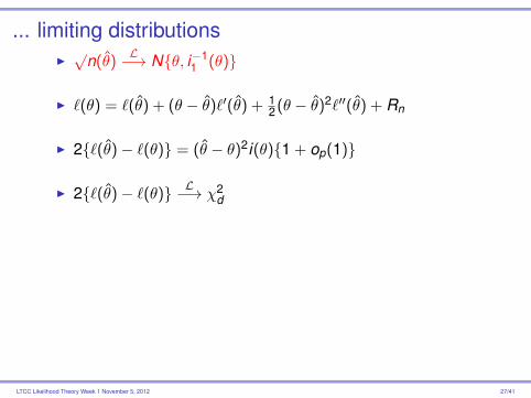
... limiting distributionsI√

n(θ)L−→ N{θ, i−1

1 (θ)}

I `(θ) = `(θ) + (θ − θ)`′(θ) + 12(θ − θ)2`′′(θ) + Rn

I 2{`(θ)− `(θ)} = (θ − θ)2i(θ){1 + op(1)}

I 2{`(θ)− `(θ)} L−→ χ2d


Inference from limiting distributionsI θ

.∼ Nd{θ, j−1(θ)} j(θ) = −`′′(θ; y)I “θ is estimated to be 21.5 (95% CI 19.5− 23.5)”I 19.5 21.5 23.5 θ ± 2σ

I w(θ) = 2{`(θ)− `(θ)} .∼ χ2d

I “likelihood based CI for θ with confidence level 95% is(18.6,23.0)” 18.6 21.5 23.0

16 17 18 19 20 21 22 23

−4

−3

−2

−1

0

log−likelihood function

θθ

log−

likel

ihoo

d

θθθθ

θθ −− θθ

1.92 w


... inference from limiting distributionsI pivotal quantities and p-value functions; θ scalarI

ru(θ) = U(θ)j−1/2(θ).∼ N(0,1)

I

Pr{U(θ)j−1/2(θ) ≤ u(θ)j−1/2(θ)} .= Φ{u(θ)j−1/2(θ)}I under sampling from the model f (y ; θ) = f (y1, . . . , yn; θ)I

pu(θ) = Φ{u(θ)j−1/2(θ)}p-value function (of θ, for fixed data)

I shorthand

= Φ{ru(θ)},and= Φ{re(θ)},= Φ{r(θ)}

are all p-value functions for θ, based on limiting dist’nsLTCC Likelihood Theory Week 1 November 5, 2012 29/41

ExampleI f (yi ; θ) = θe−yiθ, i = 1, . . . ,n

I `(θ) =

I `′(θ) =

I `′′(θ) =

I ru(θ) =√

n( 1θy − 1)

I re(θ) =√

n(1− yθ)

I r(θ) =


ExampleI f (yi ; θ) = θyi e−θ/yi !

I `(θ) =

I `′(θ) =

I `′′(θ) =

I re(θ) = (s − nθ)/√

s

I Pr(S ≤ s) 6= 1− Pr(S ≥ s)

I upper and lower p-value functions: Pr(S < s), Pr(S ≤ s)

I mid p-value function: Pr(S < sr) + 0.5Pr(S = s)


AsideI for inference re θ, given y , plot p(θ) vs θ

I for p-value for H0 : θ = θ0, compute p(θ0)

I for checking whether, e.g. Φ{re(θ)} is a goodapproximation,

I compare p(θ) = Φ{re(θ)} to pexact(θ), as a function of θ,fixed y

I or compare p(θ0) to pexact(θ0) as a function of y

I if pexact(θ) not available, simulate


Nuisance parametersI θ = (ψ, λ) = (ψ1, . . . , ψq, λ1, . . . , λd−q)

I U(θ) =

(Uψ(θ)Uλ(θ)

), Uλ(ψ, λψ) = 0

I i(θ) =

(iψψ iψλiλψ iλλ

)j(θ) =

(jψψ jψλjλψ jλλ

)I i−1(θ) =

(iψψ iψλ

iλψ iλλ

)j−1(θ) =

(jψψ jψλ

jλψ jλλ

).

I iψψ(θ) = {iψψ(θ)− iψλ(θ)i−1λλ (θ)iλψ(θ)}−1,

I `P(ψ) = `(ψ, λψ), jP(ψ) = −`′′P(ψ)


Inference from limiting distributions, nuisanceparameters

wu(ψ) = Uψ(ψ, λψ)T{iψψ(ψ, λψ)}Uψ(ψ, λψ).∼ χ2

q

we(ψ) = (ψ − ψ){iψψ(ψ, λ)}−1(ψ − ψ).∼ χ2

q

w(ψ) = 2{`(ψ, λ)− `(ψ, λψ)} = 2{`P(ψ)− `P(ψ)} .∼ χ2q;

Approximate Pivots

ru(ψ) = `′P(ψ)jP(ψ)1/2 .∼ N(0,1),

re(ψ) = (ψ − ψ)jP(ψ)1/2 .∼ N(0,1),

r(ψ) = sign(ψ − ψ)2{`P(ψ)− `P(ψ)} .∼ N(0,1)


Properties of likelihood functions and likelihoodinference

I the likelihood depends only on the minimal sufficientstatistic

I recall:L(θ; y) = m1(s; θ)m2(y) ⇐⇒ s is minimal sufficient

I equivalentlyL(θ; y)

L(θ0; y)depends only on s

I “ the likelihood map is sufficient” Fraser & Naderi, 2006;Barndorff-Nielsen, et al, 1976

i.e y → L0(·; y), or y → L(·; y) normed


... propertiesI maximum likelihood estimates are equivariant: h(θ) = h(θ)

for one-to-one h(·)I question: which of we, wu, w are invariant under

reparametrization of the full parameter: ϕ(θ)?I question: which of re, ru, r are invariant under

interest-respecting reparameterizations(ψ, λ)→ {ψ, η(ψ, λ)}?

I consistency of maximum likelihood estimate?I equivalence of maximum likelihood estimate and root of

score equation?

I observed vs. expected information


Asymptotics for Bayesian inferenceI π(θ | y) =

exp{`(θ; y)}π(θ)∫exp{`(θ; y)}π(θ)dθ

I expand numerator and denominator about θ, assuming`′(θ) = 0

I π(θ | y).

= N{θ, j−1(θ)}

I expand denominator only about θ

I result

π(θ | y).

=1

(2π)d/2 |j(θ)|+1/2 exp{`(θ; y)− `(θ; y)}π(θ)

π(θ)


Likelihood and Asymptotic Theory for Statistical Inference · 3.Likelihood inference for complex...

Documents

Transcript of Likelihood and Asymptotic Theory for Statistical Inference · 3.Likelihood inference for complex...