Likelihood Inference for Dynamic LinearModels with Markov Switching Parameters:

On the Efficiency of the Kim Filter

Kyu Ho Kang∗

Young Min Kim†

February 2017

Abstract

The Kim filter (KF) approximation is commonly used for the likelihood calcula-tion of dynamic linear models with Markov regime-switching parameters. Despiteits popularity, its approximation error has not been examined in a rigorous wayyet. This study investigates the reliability of the KF approximation. To measurethe approximation error, we compare the outcomes of the KF method with thoseof the auxiliary particle filter (APF). The APF is a numerical method requiring alonger computing time, but its error can be sufficiently minimized by increasingsimulation size. We conduct extensive simulation and empirical studies for compar-ison purposes. According to our experiments, the likelihood values obtained fromthe KF approximation are practically identical to those of the APF, and the KFmethod becomes more reliable when regimes are more persistent. Consequently,the KF approximation is a fast and efficient approach for maximum likelihoodestimation of regime-switching dynamic linear models. This article contributes tothe literature by providing evidence to justify the use of the KF method.

(JEL classification: C22, C63)

Keywords : State space model, auxiliary particle filter, Kalman filter, maximum like-lihood estimation

∗Department of Economics, Korea University, Seoul, South Korea, E-mail: kyuho@korea.ac.kr, Tel:+82-2-3290-5132†Corresponding author, Department of Economics, Korea University, Seoul, South Korea, E-mail:

eccentricecon@korea.ac.kr, Tel: +82-2-3290-2200

1

1 Introduction

Dynamic linear models with Markov regime-switching parameters are widely used in

empirical macroeconomics and finance because of their flexibility. This flexibility is

attributed to two types of unobserved state variables in the model: continuous latent

variables following an autoregressive process and discrete latent variables governed by a

first-order Markov process. This class of models includes the regime-switching dynamic

common factor, time-varying parameter, and unobserved component models. These

models are particularly useful for detecting drastic regime changes in business cycles.

Business cycles can be empirically characterized by a dynamic common factor among

various coincident macroeconomic variables. The asymmetric nature of expansions and

contractions or volatility reduction in the business cycles can be modeled by allowing the

common factor dynamics to be subject to regime shifts according to a Markov process.

For statistical inference, maximum likelihood estimation (MLE) is typically employed

in a classical approach. However, the exact likelihood calculation of the Markov regime-

switching dynamic linear models is challenging. The source of the problem is that

the conditional density of observations is not expressed in a closed form because the

conditional density of continuous latent variables depends on the entire history of the

discrete state variables.

To resolve this problem, the Kim filter (KF) approximation was proposed in the work

of Kim (1994). For convenience, we refer to continuous and discrete state variables as

factors and regimes, respectively. The key idea behind the KF method is to approximate

the conditional density of the factors, so that it depends only on the distribution of

the most recent regimes, and not on their entire history. The KF method makes the

likelihood calculation feasible, and it is easy to implement practically. Therefore, a

number of studies including Kahn and Rich (2007), Timmermann (2001), Morley and

Piger (2012), Kang, Kim, and Morley (2009), and Chauvet (1998) have employed this

approximation method for MLE of regime-switching dynamic linear models.

This work is motivated by the fact that the approximation error has not been in-

vestigated rigorously despite the popularity of the KF method. The primary goal of

2

this study is to test whether the KF method is efficient for the likelihood computation.

To this end, we measure its approximation error by comparing outcomes from the KF

method with those from the auxiliary particle filter (APF) method. The APF, intro-

duced by Pitt and Shephard (1999), relies on a numerical integration, and its numerical

error can be sufficiently minimized by increasing simulation size.1 As the difference be-

tween the likelihood values from the KF and APF methods is smaller, the KF method

is regarded as more efficient. It should be noted that using the APF is not desirable for

MLE because this numerical method requires a much longer computing time than the

KF method.

This idea of comparing the KF and APF methods is based on the work of Herbst

and Schorfheide (2015), in which the Kalman filter and particle filtering for dynamic

linear models without regime shifts are compared. We conduct extensive simulation and

empirical studies for the comparison. In the simulation study, the likelihood inference

of the methods of dynamic common factor, time-varying parameter, and unobserved

component models with Markov switching parameters is evaluated in terms of accuracy

and computing time given the simulated data. The models considered in the empirical

application are Friedman’s plucking model and a business cycle turning points model.

According to our experiments, the likelihood values obtained from the KF approx-

imation are almost identical to those of the APF method, which is robust to model

specification and sample size. Because the KF algorithm is simpler, and easier to im-

plement in practice than the APF method, the KF approximation is a fast and efficient

approach for MLE. Our work contributes to the literature on regime-switching dynamic

linear models by providing evidence to justify the use of the KF method. However, it

should be noted that the performance of the KF method tends to be less reliable as

regime shifts are more frequent. By a Monte Carlo simulation, we show that the KF

approximation error has a larger variance when regimes are less persistent.

The rest of this paper is organized as follows. In Section 2, we present a general

1Many studies on a Bayesian framework have applied the APF for the likelihood computation,given the model parameters. For instance, Chib, Nardari, and Shephard (2002) developed the APFfor a stochastic volatility model that can be expressed in a state-space model with exogenous andindependent switching parameters. Recently, Kang (2014) extended his APF algorithm for dynamiclinear models with endogenous Markov regime-switching parameters.

3

specification of our dynamic linear models with Markov switching parameters considered

in this paper. Section 3 describes the KF and APF methods for likelihood inference.

Sections 4 and 5 provide the results of KF approximation error evaluations based on

various simulation and empirical applications. The conclusion is presented in Section 6.

2 Model Framework

We consider a joint stochastic process, (yt, βt, st) where yt is a q×1 vector of observable

dependent variables and βt is a k × 1 vector of continuous state variables at time t. st

is a discrete latent regime-indicator taking one of the values {1, 2, ..., N} where N is

the number of regimes. The state variables, (βt, st), are unobserved in general. st = j

indicates that the dependent and state variables are drawn from the jth regime at time

t. Assume that Ft−1 denotes the history of the observation sequence up to time t − 1

and xt is a h × 1 vector of the predetermined or strictly exogenous variables. We then

assume that at each time t, st, βt, and yt are sequentially, not simultaneously, generated

from the following dynamic linear model with regime-switching parameters:

st|P ∼Markov(s0,P), (1)

βt|βt−1,Θ, st ∼ N (µst +Gstβt−1, Qst), (2)

yt|Ft−1,Θ, βt, st ∼ N (Hstβt + Fstxt, Rst) (3)

where s0 is the initial regime at time 0, N (·, ·) denotes the multivariate normal distri-

bution, and

Θ = {Hst , Fst , Rst , µst , Gst , Qst}Nst=1

is the set of model parameters in the transition equation (2) and measurement equation

(3). For generality, we allow all parameters to change over time depending on the regime.

The regime st is governed by a first-order finite-state Markov process with a transition

probability matrix,

P =

p11 p12 · · · p1Np21 p22 · · · p2N...

.... . .

...pN1 pN2 · · · pNN

, (4)

4

where pij = Pr[st = j|st−1 = i] is the transition probability from regime st−1 = i to

regime st = j, and∑N

j=1 pij = 1 for all i = 1, 2, .., N . Without loss of generality, we

assume that the transition probabilities are constant over time.

Once regime st is generated given st−1 independently of the history of the factors and

endogenous variables, {βi, yi}t−1t=0, βt follows a first-order vector-autoregressive (VAR(1))

process in equation (2). The regime-dependent intercept, VAR coefficients, and factor

shock variance-covariance are denoted by µst : k × 1, Gst : k × k, and Qst : k × k,

respectively.

Conditioned on the factors and regimes at time t, the dependent variable yt is nor-

mally distributed as in equation (3). The marginal impact of the factors on the depen-

dent variable is captured by Hst : q × k. Fst is a q × h coefficient matrix of xt, and Rst

is a q × q variance-covariance matrix of the measurement errors.

Our model specification is completed by initializing the state variable and regime,

(β0, s0) at time 0. First, given the transition probability matrix P, the initial regime

is assumed to be generated from its unconditional distribution if the Markov-regime

process is ergodic. That is, s0 = j is drawn with the steady-state probability,Pr [s0 = 1]Pr [s0 = 2]

...Pr [s0 = N ]

=(P′P

)−1P′[

0N×11

]: N × 1 (5)

where

P =

[IN −P′

1′N

]: (N + 1)×N.

For N = 2, the unconditional probabilities are simply obtained as

Pr[s0 = 1] =1− p22

2− p11 − p22, (6)

Pr[s0 = 2] = 1− Pr[s0 = 1].

If all regimes are transient as in a changepoint process, then s0 is fixed at one.

Finally, given the initial regime s0, the initial factors are generated differently, de-

pending on whether the factor process is stationary or nonstationary. When it is station-

5

ary, β0 is assumed to be distributed as its unconditional distribution of βt conditioned

on the initial state s0 = j as

β0|Θ,s0 = j ∼ N (βj0, P

j0 ) (7)

where βj0 is a k× 1 unconditional mean vector and P j

0 is a k× k unconditional variance-

covariance matrix of βt. Suppose that Ik denotes the k × k identity matrix, ⊗ is the

Kronecker product, and vec(·) is the vectorization of a matrix. (βj0, P

j0 ) can then be

derived as

βj0 = (Ik −Gs0=j)

−1µs0=j,

P j0 = (Ik −Gs0=j ⊗Gs0=j)

−1vec(Qs0=j),

respectively. On the other hand, if βt is nonstationary, β0 = βj0 is treated as an additional

regime-independent parameter to be estimated. As β0 is no longer a random variable,

its variance-covariance matrix, P0 = P j0 should be fixed at a k × k zero matrix.

3 Likelihood Inference

If the regimes are non-stochastic and observable, the state-space model presented in

equations (2) and (3) is linear and Gaussian, and the Kalman filter is applicable for

the exact likelihood calculation. The unobservability of regimes, however, makes the

transition equation nonlinear and the likelihood computation analytically infeasible via

the Kalman filter.

To elaborate on the source of infeasibility, let Y = {yt}Tt=1 denote a sequence of

observations. Conditioned on (Ft−1,Θ,P), by integrating out the current continuous

and discrete state variables (st, βt), the log likelihood log f(Y|Θ,P) can be obtained by

the sum of the log likelihood densities over time:

f(yt|Ft−1,Θ,P) =

∫f (yt|st, βt,Ft−1,Θ,P) p (st, βt|Ft−1,Θ,P) d (st, βt) , (8)

and log f(Y|Θ,P) =T∑t=1

log f(yt|Ft−1,Θ,P). (9)

6

The conditional density of (st, βt) is then computed by integrating over the entire history

of the state variables {(si, βi)}t−1i=0 because the factor process is regime-dependent and

p (st, βt|Ft−1,Θ,P)

=

∫p (st, βt|Ft−1,Θ,P,st−1, βt−1) p (st−1, βt−1|Ft−1,Θ,P) d (st−1, βt−1)

=

∫p (βt|Ft−1,Θ,P,st, st−1, βt−1) p (st|P,st−1)

× p (st−1, βt−1|Ft−1,Θ,P) d (st−1, βt−1) ,

p (st−1, βt−1|Ft−1,Θ,P)

=

∫p (βt−1|Ft−1,Θ,P,st−1, st−2, βt−2) f(yt|Ft−2,Θ,P)

× p (st−1|P,st−2) p (st−2, βt−2|Ft−2,Θ,P) d (st−2, βt−2) ,

p (st−2, βt−2|Ft−2,Θ,P)

=

∫p (βt−2|Ft−2,Θ,P,st−2, st−3, βt−2) f(yt−2|Ft−3,Θ,P)

× p (st−2|P,st−3) p (st−3, βt−3|Ft−3,Θ,P) d (st−3, βt−3) ,

...

As a result, the conditional density of the observations yt, f(yt|Ft−1,Θ,P) should

be obtained by integrating over the entire history of the state variables up to time t.

Because of this high dimensionality, the exact likelihood calculation is not feasible in

general.

To overcome the computational difficulty, we can consider two approaches that rely

on different approximation methods for the likelihood inference. One approach is the

Kim filter, which is the approximate Kalman filter algorithm. The key idea of this

method is to collapse N ×N possible regimes into N possible regimes at each filtering

recursion by approximation. Consequently, the conditional density of the factor βt de-

pends on (st, st−1, βt−1), not ({si}ti=0, {βi}t−1i=0) at each iteration of the recursions. The

other approach is a sequential Monte Carlo method, which is widely used for the like-

lihood inference of nonlinear state space models. As one of the sequential Monte Carlo

algorithms, the APF is implemented recursively to update the distribution of (st, βt)

conditional on the current information at time t using a set of particles with appropriate

7

weights. The following subsections provide a detailed discussion of the KF and APF

methods.

3.1 Kim Filter

The KF algorithm consists of three steps: the conditional Kalman filter, Hamilton filter,

and approximation. Given (Y,Θ,P), the log likelihood ln f (Y|Θ,P) is initialized at

zero. At time t = 0, the initial unobserved state variables distribution, p (s0, β0|Θ,P),

is given at the unconditional probability discussed in Section 2. For t = 1, 2, . . . , T , the

details of the KF algorithm steps for calculating the likelihood function are presented

as follows.

Algorithm 1: Likelihood Inference from the Kim Filter

Step 1: (Conditional Kalman Filter) The objective of the conditional Kalman filter step

is to obtain the inference of βt conditional on (st−1 = i, st = j) and information up

to time t. By running the Kalman filters for each pair of (st, st−1), the necessary

quantities are recursively computed as

E[βt|Ft−1,Θ,st = j, st−1 = i] = β(i,j)t|t−1 = µj +Gjβ

it−1|t−1, (10)

V ar[βt|Ft−1,Θ,st = j, st−1 = i] = P(i,j)t|t−1 = GjP

it−1|t−1G

′j +Qj, (11)

E[yt|Ft−1,Θ,st = j, st−1 = i] = y(i,j)t|t−1 = yt −Hjβ

(i,j)t|t−1 − Fjxt, (12)

V ar[yt|Ft−1,Θ,st = j, st−1 = i] = f(i,j)t|t−1 = HjP

(i,j)t|t−1H

′j +Rj, (13)

E[βt|Ft,Θ,st = j, st−1 = i] = β(i,j)t|t = β

(i,j)t|t−1 +K

(i,j)t (yt − y(i,j)t|t−1), (14)

V ar[βt|Ft,Θ,st = j, st−1 = i] = P(i,j)t|t = P

(i,j)t|t−1 −K

(i,j)t H ′jP

(i,j)t|t−1 (15)

where βit−1|t−1 = E[βt|Ft−1,Θ,st−1 = i] and P i

t−1|t−1 = V ar[βt|Ft−1,Θ,st−1 = i]

are the conditional expectation and variance-covariance matrix of βt given (Ft−1,

Θ, st−1 = i), respectively. K(i,j)t is the Kalman gain conditioned on st = j and

st−1 = i for i, j = 1, 2, . . . , N, which is given by

K(i,j)t = P

(i,j)t|t−1H

′j(f

(i,j)t|t−1)

−1.

8

Step 2: (Hamilton Filter) In this step, we apply the Hamilton filter (Hamilton (1989))

to obtain the likelihood density (i.e., f(yt|Ft−1,Θ,P)) and the filtered probabil-

ities (i.e., f(st, st−1|Ft,Θ,P) and f(st|Ft,Θ,P)). Given f(st−1|Ft−1,Θ,P), the

following quantities can be sequentially computed:

f(st, st−1|Ft−1,Θ,P) = Pr[st|st−1]f(st−1|Ft−1,Θ,P), (16)

f(yt|Ft−1,Θ,P) =∑st

∑st−1

f(yt|Ft−1,Θ,st, st−1)f(st, st−1|Ft−1,Θ,P), (17)

f(st, st−1|Ft,Θ,P) =f(yt|Ft−1,Θ,st, st−1)f(st, st−1|Ft−1,Θ,P)

f(yt|Ft−1,Θ,P), (18)

f(st|Ft,Θ,P) =∑st−1

f(st, st−1|Ft,Θ,P), (19)

where the conditional density of yt

f(yt|Ft−1,Θ,st = j, st−1 = i) = N(yt|y(i,j)t|t−1, f

(i,j)t|t−1

)can be computed using equations (12) and (13). Equation (16) is the predictive

probability of the regimes and equations (18) and (19) are the filtered probabilities.

Step 3: (Numerical Error) The filtered probabilities are used in the next step when

integrating out the lagged regimes to obtain the filtered factors conditioned on

the current regime only. If the filtered probabilities are too close to zero, these

values could be taken to be zero and the KF does not work because the filtered

probabilities are used as denominators in the next step. To avoid this numerical

problem, we replace the filtered probabilities by 10−4 whenever they are less than

this value.

Step 4: (Approximation) In this step we derive the filtered distribution of the factor βt

conditioned on the current regime st,

βt|Ft,Θ,P,st.

Given the normality assumption and the filtered probabilities, the KF algorithm

provides the conditional expectation and variance-covariance of the factors as fol-

9

lows:2

βjt|t = E[βt|Ft,Θ,P,st = j]

=

∑Mi=1 f(st = j, st−1 = i|Ft,Θ,P)β

(i,j)t|t

f(st = j|Ft,Θ,P), (20)

P jt|t = V ar[βt|Ft,Θ,P,st = j]

=

∑Mi=1 f(st = j, st−1 = i|Ft,Θ,P)[P

(i,j)t|t + (βj

t|t − β(i,j)t|t )(βj

t|t − β(i,j)t|t )′]

f(st = j|Ft,Θ,P). (21)

Note that the filtered density p(βt|Ft,Θ,P,st = j) is a mixture of Nt = N ×Nt−1

states where Nt−1 is the total number of regime sequences up to time t− 1. This

step is referred to as the approximation stage because (βjt|t, P

jt|t) are calculated by

integrating over st−1, not {si}t−1i=0. These filtered values are necessary when running

the conditional kalman filter step the following time.

Step 5: If t < T , set t = t+ 1 and go to Step 1; otherwise go to Step 6.

Step 6: (Log likelihood) Return the log likelihood

ln f (Y|Θ,P) =T∑t=1

ln f(yt|Ft−1,Θ,P) (22)

where the conditional density f(yt|Ft−1,Θ,P) is calculated in equation (17).

3.2 Auxiliary Particle Filter

The essential step in the likelihood inference is updating the conditional distribution

of the regimes and factors given the current information at time t. The APF is a

class of simulation-based methods that recursively update the information contained

in the current observations yt to the predictive distribution, (st, βt) |Ft−1,Θ,P. This

filtering procedure uses the sampling importance resampling method, which consists

of two stages. The first stage is to propose candidate values of the state variables.

The second stage is to reweigh them to produce draws from the target distribution,

p (st, βt|Ft,Θ,P). Per the Bayes theorem, the target density is proportional to the

2For the details of the derivation, refer to Kim and Nelson (1999b).

10

product of the conditional density of yt and the predictive density of (st, βt) .:

p (st, βt|Ft,Θ,P) ∝ f (yt|st, βt,Ft−1,Θ,P) p (st, βt|Ft−1,Θ,P) .

The key step in the APF method is to introduce an auxiliary variable, denoted by g,

where g indicates the conditional distribution of (st, βt) given the gth samples (s(g)t−1, β

(g)t−1)

and (Ft−1,Θ,P). The APF algorithm enables us to sample from

st, βt, g|Ft,Θ,P,

and return the filtered distribution, st, βt|Ft,Θ,P.

Supose that the M samples {s(g)t−1, β(g)t−1}Mg=1 drawn from

st−1, βt−1|Ft−1,Θ,P

are given, and that (s(g)t , β

(g)t ) comprise the mode of the transition distribution of (st, βt),

st, βt|s(g)t−1, β(g)t−1,Ft−1,Θ,P

conditioned on (s(g)t−1, β

(g)t−1, Ft−1, Θ, P) for each g = 1, 2, ..,M.

The first stage is to propose R values for g generated by a proposal distribution

whose mass function is given by

q (g|Ft,Θ,P) ∝ f(yt|s(g)t , β

(g)t ,Ft−1,Θ,P

).

In the second stage, we draw {s∗(r)t , β∗(r)t }Rr=1 from the predictive distribution,

st, βt|Ft−1,Θ,P.

Then, for each r = 1, 2, .., R, we calculate the second importance weights,

wr ∝f(yt|s∗(r)t , β

∗(r)t ,Ft−1,Θ,P

)f(yt|s(gr)t , β

(gr)t ,Ft−1,Θ,P

) (23)

where {gr}Rr=1 is a set of indices sampled from the M draws of g. Finally, we resample

M draws for (st, βt) with the second importance weights from {s∗(r)t , β∗(r)t }Rr=1. The re-

11

sampled M draws are taken as the samples from the filtered distribution, st, βt|Ft,Θ,P.

Given (Y,Θ,P) and (M,R), the initial particles {s(g)0 , β(g)0 }Mg=1 are drawn from

s0, β0|Θ,P, which is the unconditional probability as we discussed in Section 2. For

each time point t, the steps of the APF algorithm can be summarized as follows.

Algorithm 2: Auxiliary Particle Filter

Step 1: Obtain the mode of the proposal distribution ( st, βt), compute the first stage

weights, and sample auxiliary variables.

Step 1-(a): Given P, sample {s(g)t−1, β(g)t−1}Mg=1 from st−1, βt−1|Ft−1,Θ,P, and {u(g)t }Mg=1 ∼

Unif(0, 1). Then, determine s(g)t as

s(g)t = 1 if u

(g)t < p1, (24)

s(g)t = 2 if u

(g)t ≥ p1

where p1 = p11 if s(g)t−1 = 1, and p1 = p21 if s

(g)t−1 = 2.

Step 1-(b) Given Θ, {s(g)t , β(g)t−1}Mg=1, and (yt, xt), calculate β

(g)t as

β(g)t = E

[βt|β(g)

t−1, s(g)t ,Θ

]= µ

s(g)t

+Gs(g)tβ(g)t−1, (25)

Step 1-(c) Compute the first stage weights,

wg ∝ Nq

(yt|Hs

(g)tβ(g)t + F

s(g)txt, Rs

(g)t

)(26)

Step 1-(d): Draw {gr}Rr=1 from the indices g = 1, ...,M with the probability mass

proportional to

w∗g =wg∑Mg=1wg

, (27)

and associate sampled index with {s(gr)t−1 , β(gr)t−1 }Rr=1 and {s(gr)t , β

(gr)t }Rr=1.

Step 2: Generate s∗t , β∗t from the transition densities, compute the second stage weights,

and resample ( st, βt).

12

Step 2-(a): Given {s(gr)t−1}Rr=1, P, and {u(r)t }Rr=1 ∼ unif(0, 1), sample

s∗(r)t = 1 if u

(r)t < p1, (28)

s∗(r)t = 2 if u

(r)t ≥ p1

where p1 = p11 if s(gr)t−1 = 1, and p1 = p21 if s

(gr)t−1 = 2.

Step 2-(b): Given {s∗(r)t , β(gr)t−1 }Rr=1 and Θ, simulate

β∗(r)t ∼ Nk

(µs∗(r)t

+Gs∗(r)tβ(gr)t−1 , Qs

∗(r)t

). (29)

Step 2-(c): Compute the second importance weights,

wr ∝Nq

(yt|Hs

∗(r)tβ∗(r)t + F

s∗(r)txt, Rs

∗(r)t

)Nq

(yt|Hs

(gr)tβ(gr)t + F

s(gr)txt, Rs

(gr)t

) . (30)

Step 2-(d): Resample M times from the R draws with the probability mass,

w∗r =wr∑Rr=1wr

. (31)

The resampled draws are the filtered samples {s(g)t , β(g)t }Mg=1 from st, βt|Ft,Θ,P.

Given the filtered samples {s(g)t−1, β(g)t−1}Mg=1 from

st−1, βt−1|Ft−1,Θ,P,

it is straightforward to sample the predictive draws, {s(g)t , β(g)t }Mg=1 from st, βt|Ft−1,Θ,P.

Once the predictive draws for (st, βt) are simulated, we can compute the one-step-ahead

conditional density of yt,

f (yt|Ft−1,Θ,P) =

∫f (yt|st, βt,Ft−1,Θ,P) p (st, βt|Ft−1,Θ,P) d (st, βt) (32)

by using the simple Monte Carlo averaging of Nq (yt|Hstβt + Fstxt, Rst) over the predic-

tive draws.

13

Given (Y,Θ,P), the log likelihood ln f (Y|Θ,P) is initialized at zero. At time t = 0,

initial particles {s(g)0 , β(g)0 }Mg=1 are drawn from the unconditional probability as discussed

in Section 2. For t = 1, 2, .., T , the APF algorithm steps are summarized as follows.

Algorithm 3: Likelihood Inference using the Auxiliary Particle Filter

Step 1: Simulate the predictive density of (st, βt) and calculate the likelihood density.

Step 1-(a): Given {s(g)t−1}Mg=1, {u(g)t }Mg=1 ∼ Unif(0, 1), and P, predictive values of st are

drawn from

s(g)t = 1 if u

(g)t < p1, (33)

s(g)t = 2 if u

(g)t ≥ p1

where p1 = p11 if s(g)t−1 = 1, and p1 = p21 if s

(g)t−1 = 2.

Step 1-(b): Conditioned on {s(g)t , β(g)t−1}Mg=1 and Θ, draw predictive values of βt from

β(g)t ∼ Nk

(µs(g)t

+Gs(g)tβ(g)t−1, Qs

(g)t

)(34)

Step 1-(c): Compute the one-step-ahead predictive density of yt by a numerical inte-

gration as

f (yt|Ft−1,Θ,P) ' 1

M

M∑g=1

Nq

(yt|Hs

(g)tβ(g)t + F

s(g)txt, Rs

(g)t

). (35)

Step 2: Apply Algorithm 2 and sample {s(g)t , β(g)t }Mg=1 from st, βt|Ft,Θ,P. If t < T , set

t = t+ 1 and go to Step 1; otherwise go to Step 3.

Step 3: Return the log likelihood,

ln f (Y|Θ,P) =T∑t=1

ln f (yt|Ft−1,Θ,P) . (36)

Note that given the parameters we can obtain the filtered probabilities of the regimes

and filtered factors over time by averaging {s(g)t , β(g)t }Mg=1 drawn from st, βt|Ft,Θ,P in

Step 2.

14

4 Simulation Study

The KF approximation method is evaluated based on simulation studies and empirical

applications in comparison with the APF method. We begin by measuring the approxi-

mation error of the KF method using simulated data. We consider three representative

examples of dynamic linear models with Markov switching parameters, which can be

expressed as special cases of the general model specification in Section 2.

4.1 Models

4.1.1 Dynamic Common Factor Model with Markov Switching Parameters

The first specification is a dynamic common factor model with Markov switching pa-

rameters. This model specification is widely used to empirically characterize business

cycles by a dynamic factor βt among multiple observed variables yt. The dynamic factor

is subject to regime shifts modeled by a Markov process st. At time t, (st, βt, yt) are

sequentially, not simultaneously, generated from the following generic dynamic linear

model with regime-switching parameters:

st|P ∼Markov(s0,P), (37)

βt|βt−1,Θ, st ∼ N (Gstβt−1, Qst),

yt|Ft−1,Θ, βt, st ∼ N (Hstβt, Rst).

The transition matrix for regime st is given by

P =

[p11 1− p11

1− p22 p22

].

Throughout Sections 4 and 5, we assume that the regime st is governed by a two-state

first-order Markov process, in which all regimes are recurrent.3

For data simulation, bivariate observations yt are generated by one common factor

3In the estimation of regime-switching models, regime identification is an important issue. However,the focus of this paper is the likelihood inference given the parameters. For this reason we do notdiscuss the label switching problem.

15

(i.e., k = 1). Our choice of parametrization is given by

st = 1 st = 2Gst 0.5 0.9Qst 1 3Hst ( 1 −0.5 )′ ( 1 0.5 )′

Rst 1× I2 4× I2

In this parametrization, the common factor process is regime-dependent. Particularly,

the factor is more persistent and volatile in regime 2. Further, the factor loadings and

measurement shock variance differ in different regimes.

4.1.2 Time-Varying Parameter Model with Markov Switching Parameters

Consider the case in which there is a possibility of gradual changes in linear regression

coefficients over time along with regime shifts in the coefficient process or volatility.

This can be easily modeled by a time-varying parameter model with Markov switching

parameters as follows:

βt|βt−1,Θ, st ∼ N (βt−1, Qst), (38)

yt|Ft−1,Θ, βt, st ∼ N (Htβt, Rst)

where Ht ∼ Unif(0, 2) is a covariate uncorrelated with the measurement errors. We

fix the measurement error variance and parameter shock variance such that Qst=1 =

Rst=1 = 1, Qst=2 = 5, and Rst=2 = 3. As the variances in regime 2 are larger than in

regime 1, the simulated data is supposed to reveal more drastic coefficient changes and

higher volatility during the period corresponding to the second regime.

4.1.3 Unobserved Component Model with Markov Switching Parameters

In an unobserved component model the observed time series data is decomposed into the

stochastic trend and cyclical components. The trend component is typically assumed

to be a random walk process, and the cyclical component follows a stationary vector

16

autoregressive process. We consider a simple specification:

βt|βt−1,Θ, st ∼ N (µst +Gstβt−1, Qst),

yt|Ft−1,Θ, βt, st ∼ N (βt, Rst)

where yt is univariate and assumed to be the sum of a first-order autoregressive process

and a white noise component. These unobserved components are identified as the dif-

ference in persistence. We set the parameters as presented below, so that the dependent

variable is more persistent and volatile under regime 2.

st = 1 st = 2µst 2 1Gst 0.5 0.9Qst 1 4Rst 1 2

4.2 Likelihood Comparison

For each model, we simulate the time series of dependent variables and factors given the

true parameters. We consider five different sample sizes (T = 80, 100, 200, 400, and 800)

to see whether the size of the KF approximation error is robust to sample size. The first

and third 25% of samples are drawn under regime 1 and the others are drawn under

regime 2. For instance, in the case of T = 80, the first and third 20 observations and

factors are simulated by the parameters under regime 1, and the others under regime

2. Using the simulated data, we run the KF and APF algorithms once to compute and

compare the likelihood values at the true parameters. For the APF, resampling and

particle sizes are given by R = 50, 000 and M = 50, 000, respectively. The likelihood

values obtained from the APF with such large simulation sizes are accurate enough to

be regarded as the true likelihood values.

Table 1 presents the results of the likelihood computations. There are three important

findings in this table. First, the log likelihoods approximated by the KF method are

almost identical to those of the APF. The average approximation error is almost zero and

the maximum absolute error is 0.47 in this experiment. The KF method does not seem

to lead to a misleading likelihood ratio test. Second, the performance of the KF method

17

Table 1: Log Likelihood (ln L) and Computing Time (Time) ComparisonBetween the KF and APF methods DCF, TVP, and UC indicate the dynamic common

factor model, time-varying parameter model, and unobserved component model, respectively.

The computing time is in seconds.

(a) DCF

APF KFlnL Time lnL Time

T = 80 -328.31 615.99 -328.19 0.06T = 100 -405.52 765.89 -405.34 0.04T = 200 -803.75 1546.29 -803.65 0.07T = 400 -1633.13 3098.10 -1633.50 0.13T = 800 -3213.81 6187.61 -3214.15 0.25

(b) TVP

APF KFlnL Time lnL Time

T = 80 -184.34 585.00 -184.46 0.03T = 100 -242.13 724.21 -241.60 0.02T = 200 -469.72 1447.01 -469.94 0.03T = 400 -934.77 2921.31 -934.61 0.06T = 800 -1805.31 5780.46 -1804.92 0.11

(c) UC

APF KFlnL Time lnL Time

T = 80 -172.92 585.17 -172.97 0.01T = 100 -218.31 730.79 -218.49 0.01T = 200 -439.57 1441.91 -439.62 0.03T = 400 -883.84 2910.35 -883.65 0.05T = 800 -1713.41 5760.40 -1713.73 0.11

18

is robust to the model specifications and sample sizes as shown in the table. Third,

the computing speed of the KF method is incomparable. The APF takes hundreds of

seconds whereas the KF completes within one second. In addition, Figure 1 plots the

log conditional densities of the observations over time, and clearly indicates that the log

likelihood densities calculated by the KF method are indistinguishable from those of the

APF method. Consequently, those simulation studies strongly demonstrate that the KF

method is fast and efficient enough to be used for likelihood inference. The KF method

is a more desirable approach for likelihood function optimization than the APF method.

Another important element of approximation quality is the accuracy of the filtered

states and filtered probabilities of regimes. We report the quantities of the filtered states

and regime probabilities obtained from a single run of the KF and APF in Figures 2

and 3. These figures depict the sequence of the filtered factors and filtered probabilities

of the regimes along with the corresponding true values in the case of T=200, as an

example. There is little difference between the filtered values produced by the KF and

APF, which is a finding robust to the sample sizes.

4.3 Regime Persistence and Approximation Error

We now examine the sensitivity of the KF approximation error to regime persistence.

It is important to investigate whether the KF method successfully approximates the

historical path of the regimes regardless of regime shift frequency. To do this, we repeat

the simulation in Section 4.2 500 times with a sample size of 80. For each simulation, the

regime process is generated according to a Markov process with the following transition

matrices:

PH =

[0.98 0.020.02 0.98

]and PL =

[0.8 0.20.2 0.8

]PH and PL indicate high and low regime persistence, respectively. As a result, the

regime shifts generated by PL occur more frequently than those generated by PH . For

each of the 500 simulated data sets, we run the KF and APF and store the approximation

error,

ln f (Y|Θ,P)KF − ln f (Y|Θ,P)APF , P ∈ {PH,PL}.

19

Figure 1: Log Likelihood Densities This figure plots the log likelihood densities over

time. DCF, TVP, and UC indicate the dynamic common factor model, time-varying parameter

model, and unobserved component model, respectively. The conditional densities from the KF

and APF methods are the black dashed line and blue dotted line, respectively.

0 50 100 150 200Time

-10

-9

-8

-7

-6

-5

-4

-3

-2

-1

log-Li

kelih

ood

KF APF

(a) DCF

0 50 100 150 200Time

-7

-6

-5

-4

-3

-2

-1

0

log-Li

kelih

ood

KF APF

(b) TVP

0 50 100 150 200Time

-10

-8

-6

-4

-2

0

log-Li

kelih

ood

KF APF

(c) UC

1

20

Figure 2: Filtered Factors This figure plots the filtered factors over time for the DCF,

TVP, and UC models. The true factors, factors filtered by the KF, and factors filtered by the

APF are the black dashed line, blue solid line, and red dotted line, respectively.

0 50 100 150 200-4

-3

-2

-1

0

1

2

3

4True KF APF

(a) DCF

0 50 100 150 200-4

-2

0

2

4

6True KF APF

(b) TVP

0 50 100 150 2005

6

7

8

9

10

11

12

13 True KF APF

(c) UC

1

21

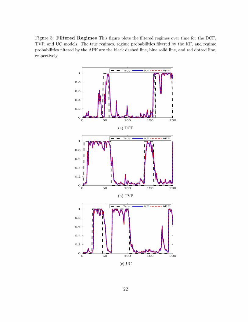
Figure 3: Filtered Regimes This figure plots the filtered regimes over time for the DCF,

TVP, and UC models. The true regimes, regime probabilities filtered by the KF, and regime

probabilities filtered by the APF are the black dashed line, blue solid line, and red dotted line,

respectively.

0 50 100 150 2000

0.2

0.4

0.6

0.8

1True KF APF

(a) DCF

0 50 100 150 2000

0.2

0.4

0.6

0.8

1True KF APF

(b) TVP

0 50 100 150 2000

0.2

0.4

0.6

0.8

1True KF APF

(c) UC

1

22

Figure 4 plots the empirical kernel densities of the 500 approximation errors, and

Table 2 reports its sample mean and standard deviation. For all models, empirical

densities are centered around zero regardless of the regime persistence. However, the

KF method seems to be more reliable when the regime is more persistent, because the

error density with PH is much sharper than that with PL. This is attributed to the

fact that approximating the entire regime path by the recent regimes is difficult when

the regime shifts are frequent and the set of potential regime paths with a high mass

is large. In short, the performance of the KF method becomes uncertain when regime

persistence is low, although it is robust to the model specification and sample size.

Table 2: Summary Statistics for Approximation Error This table presents the

mean and standard deviation (s.d.) of likelihood discrepancy between the KF and APF.

PH PL

mean s.d. mean s.d.DCF 0.0007 0.0945 0.0266 0.1797TVP 0.0149 0.1109 0.0895 0.2738UC 0.0080 0.0147 0.0147 0.2082

5 Empirical Applications

Regarding empirical studies, we consider two popular regime-switching dynamic linear

models for business cycle analysis: Friedman’s plucking model (Kim and Nelson (1999a))

and the business cycle turning points model (Kim and Nelson (1998)).

5.1 Friedman’s Plucking Model

Milton Friedman’s plucking model is one of the popular business cycle models to explain

the nature of recessions. The most distinguishing feature of this model is that business

cycles are extremely asymmetric. The time-path of the output can only move along a

potential output process. However, the output is plucked downwards at irregular inter-

vals. The plucking shocks are temporary demand shocks, whereas the fluctuations of the

potential output are driven by supply shocks. From this model’s point of view, reces-

sions are caused by uncommon negative and temporary shocks such as financial crises

23

Figure 4: Approximation Error Kernel Density This figure plots the kernel density es-

timates of likelihood discrepancy based on the KF and APF. The approximation error densities

corresponding to high and low regime persistence are the solid and dashed lines, respectively.

-1 -0.5 0 0.5 1Approximation Error

0

0.05

0.1

0.15

0.2

0.25

0.3

0.35

0.4

0.45p = 0.8p = 0.98

(a) DCF

-1 -0.5 0 0.5 1Approximation Error

0

0.05

0.1

0.15

0.2

0.25

0.3

0.35

0.4p = 0.8p = 0.98

(b) TVP

-1 -0.5 0 0.5 1Approximation Error

0

0.1

0.2

0.3

0.4

0.5p = 0.8p = 0.98

(c) UC

1

24

and oil shocks. Kim and Nelson (1999a) propose an econometric model incorporating

the asymmetric behavior of business cycles. Following Kim and Nelson (1999a), we de-

compose the log of real GDP yt into a transitory component, xt, and trend component,

zt:

yt = xt + zt (39)

where

xt = δst + φ1xt−1 + φ2xt−2 + ut, ut ∼ i.i.d.N (0, σ2u,st), (40)

zt = g + zt−1 + vt, vt ∼ i.i.d.N (0, σ2v). (41)

To identify asymmetric business cycle dynamics, we impose restrictions as follows:

δst=1 < 0, δst=2 = 0, σ2u,st=2 = 0.

The business cycle corresponds to transitory deviations in the output process away

from its permanent component. Given that the economy stays in regime 1, the transi-

tory component has a negative unconditional mean because δst=1 is constrained to be

negative. The period st = 1 can be interpreted as the state of the plucked-down econ-

omy. Meanwhile, in regime 2, the output fluctuates according to the stochastic trend

only, not the business cycle component, because the transitory shock variance, σ2u,st=2,

is equal to zero. φ1 and φ2 determine the persistence of the recession component xt. g

is a deterministic drift in trend.

The plucking model does not contain measurement error, but the measurement equa-

tion should include measurement error to apply the APF. To resolve this problem, we

should reexpress the model as another state-space form with measurement error. To do

this, we eliminate the trend component by multiplying both sides of equation (39) by

(1− L),

yt = g + xt − xt−1 + yt−1 + vt, ut ∼ i.i.d.N (0, σ2v) (42)

where L is a lag operator and

xt = δst + φ1xt−1 + φ2xt−2 + ut, ut ∼ i.i.d.N (0, σ2u,st). (43)

25

For the likelihood inference, the resulting state-space form given the regime is expressed

by

βt|βt−1,Θ, st ∼ N (µst +Gstβt−1, Qst),

yt|Ft−1,Θ, βt, st ∼ N (Hβt + Fxt, Rst)

where

βt = [ xt xt−1 ]′, µst = [ δst 0 ]′, Gst =

[φ1 φ2

1 0

], Qst = diag( σ2

u,st 0 ),

and

H = [ 1 −1 ], F = [ g 1 ], xt = [ 1 yt−1 ]′, Rst = σ2v .

We now estimate the model using the log of quarterly real GDP data for the United

States ranging from 1951:Q1 to 2016:Q1.4 This model is estimated by the MLE where

the likelihoods are computed by the KF method and the log likelihood functions are

numerically maximized. To reduce the local-maxima problem, we follow the approach of

Chib and Ramamurthy (2010) and use a simulated annealing algorithm combined with

a Newton-Raphson method. This numerical optimizer is especially useful in cases where

the likelihood is high-dimensional and irregular. Once the likelihood is maximized, the

likelihood is computed at the ML estimates using the KF and APF methods. MLE

results for the model parameters and likelihood values at the estimates are reported in

Table 3.

The log likelihood from the KF method is -567.57 and that from the APF method is

-567.29. The approximation error is measured at 0.28, so the likelihood values calculated

by the KF and APF methods are almost equal. Moreover, the estimation results are

convincing. Figures 5 and 6 plot the estimated stochastic trend and asymmetric busi-

ness cycles of the log real GDP. These estimates are the filtered values of unobserved

components (i.e., xt|t and zt|t). During the normal period, the economy is subject mostly

to permanent shocks, whereas the transitory component plays an important role in the

output fluctuations during recession. On the other hand, Figure 7 presents the filtered

4The data come from the FRED database at the Federal Reserve Bank of St. Louis. They are inbillions of chained 2009 USD with a seasonally adjusted annual rate.

26

Table 3: Parameter Estimates: Friedman’s Plucking Model This table presents

the parameter estimates, the log likelihoods (ln L), and the computing time (Time) in seconds.

Parameter Estimates t valueg 3.01 2.89δ1 -5.60 -1.18φ1 1.16 0.43φ2 -0.32 -0.49σ2v 7.19 2.94σ2u,1 0.01 0.06p11 0.61 19.99p22 0.96 15.83lnL APF -567.57

KF -567.29Time APF 386.79

KF 0.06

probabilities of recession, Pr[st = 1|Ft], along with the NBER indicator. The filtered

probabilities are strongly correlated with the NBER business cycle dates, and historical

recessions seem to be precisely detected by this plucking model.

5.2 Business Cycle Turning Points Model

The business cycle turning points model used in the work of Kim and Nelson (1998)

encompasses the two key features of business cycles: one common factor among macroe-

conomic observations containing information on the state of the economy and the regime-

switching dynamics of the common factor. To deal with these characteristics, the model

considers a dynamic common factor of economic variables and turning points of the busi-

ness cycle. Assume that yit represents the first difference of the natural log of the i-th

observed coincident indicators at time t. The observations are assumed to be generated

by one common factor, denoted by ct, and their idiosyncratic components are as follows:

yit = γict + eit, i = 1, 2, 3, 4. (44)

27

Figure 5: The log Real GDP and Estimates of the Permanent ComponentThis figure plots the log U.S. real GDP (dotted, blue) along with its stochastic trend (dashed,

black).

1960 1970 1980 1990 2000 2010Time

8

8.2

8.4

8.6

8.8

9

9.2

9.4

9.6

9.8

Trendlog Real GDP

The common factor ct and error term eit are assumed to follow an AR(1) process.

ct = δst + φct−1 + vt, vt ∼ i.i.d.N (0, σ2v), (45)

eit = ψiei,t−1 + εit, εit ∼ i.i.d.N (0, σ2i ), i = 1, 2, 3, 4 (46)

where the intercept term in the factor process, δst , is subject to regime shifts, φ deter-

mines the persistence of the common factor, σ2v is the variance of the factor shock, ψi

captures the persistence of each shock, and σ2i is the idiosyncratic shock variance. We

also assume that vt and εit are mutually independent. For the factor identification, the

first factor loading of the common factor is taken to be unity(i.e., γ1 = 1).

The dynamic common factor is extracted by the only source of comovements among

the observed macroeconomic variables, so the factor can be interpreted as the business

cycle. By allowing the intercept term δst to switch between the two regimes, we can

detect the turning points of the business cycles.

As in the plucking model, we multiply both sides of equation (44) by (1−ψiL), and

we can eliminate the serial correlation of the idiosyncratic component for consideration

28

Figure 6: Transitory Component of the log Real GDP This figure plots the cyclical

component of the log U.S. real GDP.

1960 1970 1980 1990 2000 2010Time

-30

-25

-20

-15

-10

-5

0

Cycle Component

of the measurement error in the measurement equation,

yit = ψiyi,t−1 + γict − ψict−1 + εit, i = 1, 2, 3, 4. (47)

For the likelihood inference, the resulting state-space representation is obtained as

βt|βt−1,Θ, st ∼ N (µst +Gstβt−1, Qst), (48)

yt|Ft−1,Θ, βt, st ∼ N (Hβt + Fxt, Rst)

where

βt = [ ct ct−1 ]′, µst = [ δst 0 ]′, Gst =

[φ 01 0

], Qst = diag[ σ2

v 0 ]′,

29

Figure 7: Probabilities of Recessions: Friedman’s Plucking Model This figure

plots the filtered probabilities of recession (dashed, blue) along with the NBER recession

indicator (dotted, black) over time

1960 1970 1980 1990 2000 2010

Time

-0.2

0

0.2

0.4

0.6

0.8

1

NBER RecessionProbabilities of Recession

and

H =

[1 γ2 γ3 γ4−ψ1 −ψ2γ2 −ψ3γ3 −ψ4γ4

]′,

F = diag[ ψ1 ψ2 ψ3 ψ4 ]′,

xt = [ y1,t−1 y2,t−1 y3,t−1 y4,t−1 ]′,

Rst = diag[ σ21 σ2

2 σ23 σ2

4 ]′.

The data used for estimation pertain to U.S. monthly industrial production, personal

income less transfer, manufacturing and trade sales, and non-farm employee data. The

time span is January 1967 to August 2014. Table 4 summarizes the estimates of the

model parameters and likelihood values from the KF and APF methods. Figures 8

and 9 plot the filtered common factor process and the filtered probability of recession

over time, respectively. These recession probabilities are in close agreement with the

NBER recession indicator. In addition, the asymmetric nature of business cycle phases

is captured because expansions display a longer duration on average than recessions.

30

Table 4: Parameter Estimates: Business Cycle Turning Points Model This table

presents the parameter estimates, the log likelihoods (ln L), and the computing time (Time)

in seconds.

Parameter Estimates t valueδ1 -0.17 -2.76δ2 0.16 4.18φ 0.64 9.53σ2v 0.06 5.07ψ1 0.11 2.30ψ2 -0.16 -3.81ψ3 -0.24 -5.79ψ4 -0.42 -4.73γ2 0.60 11.45γ3 0.89 11.90γ4 0.46 18.37σ21 0.32 15.86σ22 0.33 16.56σ23 0.75 16.58σ24 0.01 4.05p11 0.91 18.59p22 0.98 136.06lnL APF -1476.43

KF -1476.07Time APF 4994.36

KF 0.37

According to Table 4, the KF approximation error in this application is around

0.37, which is very small, similar to the experiment with the plucking model. This

finding also strongly supports the reliability of the KF approximation approach. We can

conclude that, although the KF approximation does not integrate the entire history of

the regimes, this method produces an accurate likelihood value that is close enough to

the exact likelihood value.

6 Conclusion

In this paper, we evaluate the KF approximation method for the likelihood inference of

dynamic linear models with Markov switching parameters. Its approximation error is

measured by the difference between the likelihood values obtained by the KF and APF

31

Figure 8: New Coincident Index This figure plots the new coincident index extracted

from the estimation of the dynamic common factor model with Markov switching parameters.

1970 1975 1980 1985 1990 1995 2000 2005 2010 2015

Time

-2

-1.5

-1

-0.5

0

0.5

1

1.5

2

BaselineNew Coincident Index

methods, given that the likelihood from the APF can be rendered sufficiently close to

the exact likelihood value obtained when using a large simulation size. According to the

likelihood comparison based on our extensive simulation and empirical studies, the KF

approximation error is sufficiently small, particularly when the regimes are persistent,

and the performance is robust to the sample size and model specifications. Therefore,

the KF method is a fast and efficient likelihood inference approach for dynamic linear

models with Markov-regime switching parameters. We believe that our work justifies

the use of the KF method in the existing literature on MLE of the models.

The KF approximation can be useful for the Bayesian posterior simulation as well.

Typically, model parameters are sampled from their full conditional distributions, given

regimes and factors. Because of the dependency on the regimes and factors, the pa-

rameter sampling efficiency is not high, especially when the models are highly nonlinear

to parameters. By using the KF method, we can optimize the likelihood or posterior

density integrating over the latent variables, and obtain a proposal distribution that

successfully approximates the posterior distribution. Consequently, we may achieve a

32

Figure 9: Probabilities of Recession: Business Cycle Turning Points ModelThis figure plots the filtered probability of recession (dashed, blue) along with the NBER

recession indicator (dotted, black) over time.

1970 1975 1980 1985 1990 1995 2000 2005 2010 2015

Time

-0.2

0

0.2

0.4

0.6

0.8

1

NBER RecessionProbabilities of Recession

high efficiency of posterior sampling. We will consider the application of the KF method

in the Bayesian posterior sampling in future work.

33

References

Chauvet, M. (1998), “An Econometric Characterization of Business Cycle Dynamics

with Factor Structure and Regime Switching,” International Economic Review, 39(4),

969–996.

Chib, S., Nardari, F., and Shephard, N. (2002), “Markov chain Monte Carlo meth-

ods for stochastic volatility models,” Journal of Econometrics, 108, PII S0304–

4076(01)00137–3.

Chib, S. and Ramamurthy, S. (2010), “Tailored Randomized-block MCMC Methods

with Application to DSGE Models,” Journal of Econometrics, 155, 19–38.

Hamilton, J. (1989), “A new approach to the economic analysis of nonstationary time

series and the business cycle,” Econometrica, 57, 357–84.

Herbst, E. and Schorfheide, F. (2015), “Bayesian Estimation of DSGE Models,” Prince-

ton University Press.

Kahn, J. A. and Rich, R. W. (2007), “Tracking the new economy: Using growth theory

to detect changes in trend productivity,” Journal of Monetary Economics, 54, 1670–

1701.

Kang, K. H. (2014), “Estimation of state-space models with endogenous Markov regime-

switching parameters,” Econometrics Journal, 17, 56–82.

Kang, K. H., Kim, C. J., and Morley, J. (2009), “Changes in U.S. Inflation Persistence,”

Studies in Nonlinear Dynamics and Econometrics, 13, 1–23.

Kim, C. J. (1994), “Dynamic linear models with Markov-switching,” Journal of Econo-

metrics, 60, 1–22.

Kim, C. J. and Nelson, C. R. (1998), “Business Cycle Turning Points, A New Coincident

Index, and Tests of Duration Dependence Based on a Dynamic Factor Model With

Regime Switching,” Review of Economics and Statistics, 80, 188–201.

34

— (1999a), “Friedman’s Plucking Model of Business Fluctuations: Tests and Fstimates

of Permanent and Transitory Components,” Journal of Money, Credit, and Banking,

31(3), 317–334.

— (1999b), “State-Space Models with Regime- Switching: Classical and Gibbs-Sampling

Approaches with Applications,” MIT Press, Cambridge.

Morley, J. and Piger, J. (2012), “The Asymmetric Business Cycle,” Review of Economics

and Statistics, 94(1), 208–221.

Pitt, M. K. and Shephard, N. (1999), “Filtering via Simulation: Auxiliary Particle

Filters,” Journal of the American Statistical Association, 94(446), 590–599.

Timmermann, A. (2001), “Structural Breaks, Incomplete Information, and Stock

Prices,” Journal of Business and Economic Statistics, 19(3), 299–314.

35