MATLAB Historical Overview Historical Overview
43
MATLAB Adapted from various sources, with main origin MathWorks Historical Overview • Short for “matrix laboratory”. • Invented in 1970’s by Cleve Moler, chairman of CS dept. at University of New Mexico. • Originally designed to provide students access to LINPACK and EISPACK without learning to LINPACK and EISPACK without learning Fortran • Numerical computing environment and programming language. • Spread to other universities and found a strong audience within the applied mathematics community. Historical Overview (cont.) • Jack Little joined Cleve and Steve Bangert to found The MathWorks in 1984 and a developed C rewrite of MATLAB. • MATLAB was first adopted by control design engineers, Little's specialty, but quickly spread to many other domains. domains. • It is now also used in education, in particular the teaching of linear algebra and numerical analysis, and is popular amongst scientists involved with image processing. • MATLAB origins video by Cleve: • http://www.mathworks.com/company/newsletters/news_notes/clevescorner/dec04.html Overview • MATLAB began with 80 functions – simple matrix calculator, portable machine graphics • NOW it has over 8000 functions • NOW it has over 8000 functions • MATLAB engines incorporated the LAPACK and BLAS libraries, embedding the state of the art software for matrix computation.
Transcript of MATLAB Historical Overview Historical Overview
MATLAB
Adapted from various sources, with main origin MathWorks
Historical Overview
• Short for “matrix laboratory”.
• Invented in 1970’s by Cleve Moler, chairman of CS dept. at University of New Mexico.
• Originally designed to provide students access to LINPACK and EISPACK without learning to LINPACK and EISPACK without learning Fortran
• Numerical computing environment and programming language.
• Spread to other universities and found a strong audience within the applied mathematics community.
Historical Overview (cont.)
• Jack Little joined Cleve and Steve Bangert to found The MathWorks in 1984 and a developed C rewrite of MATLAB.
• MATLAB was first adopted by control design engineers, Little's specialty, but quickly spread to many other domains.domains.
• It is now also used in education, in particular the teaching of linear algebra and numerical analysis, and is popular amongst scientists involved with image processing.
• MATLAB origins video by Cleve:• http://www.mathworks.com/company/newsletters/news_notes/clevescorner/dec04.html
Overview
• MATLAB began with 80 functions – simple matrix calculator, portable machine graphics
• NOW it has over 8000 functions• NOW it has over 8000 functions
• MATLAB engines incorporated the LAPACK and BLAS libraries, embedding the state of the art software for matrix computation.
Overview
• MATLAB is a high-performance language for technical computing. It integrates computation, visualization, and programming in an easy-to-use environment where problems and solutions are expressed in familiar mathematical notation. Typical uses include
• Math and computation• Math and computation
• Algorithm development
• Data acquisition
• Modeling, simulation, and prototyping
• Data analysis, exploration, and visualization
• Scientific and engineering graphics
• Application development, including graphical user interface building
Overview (cont.)
• MATLAB is an interactive system whose basic data element is an array that does not require dimensioning. This allows you to solve many technical computing problems, especially those with matrix and vector formulations, in a fraction of the time it would take to write a program in a scalar noninteractive language such write a program in a scalar noninteractive language such as C or Fortran.
• MATLAB has evolved over a period of years with input from many users. In university environments, it is the standard instructional tool for introductory and advanced courses in mathematics, engineering, and science. In industry, MATLAB is the tool of choice for high-productivity research, development, and analysis.
Overview (cont.)
• MATLAB features a family of add-on application-specific solutions called toolboxes. Very important to most users of MATLAB, toolboxes allow you to learn and apply specialized technology. Toolboxes are comprehensive collections of MATLAB functions (M-files) that collections of MATLAB functions (M-files) that extend the MATLAB environment to solve particular classes of problems. Areas in which toolboxes are available include signal processing, control systems, neural networks, fuzzy logic, wavelets, simulation, and many others.
The Main Parts
• Desktop Tools and Development Environment
• The MATLAB Mathematical Function LibraryLibrary
• The MATLAB Language
• Graphics
• MATLAB External Interfaces
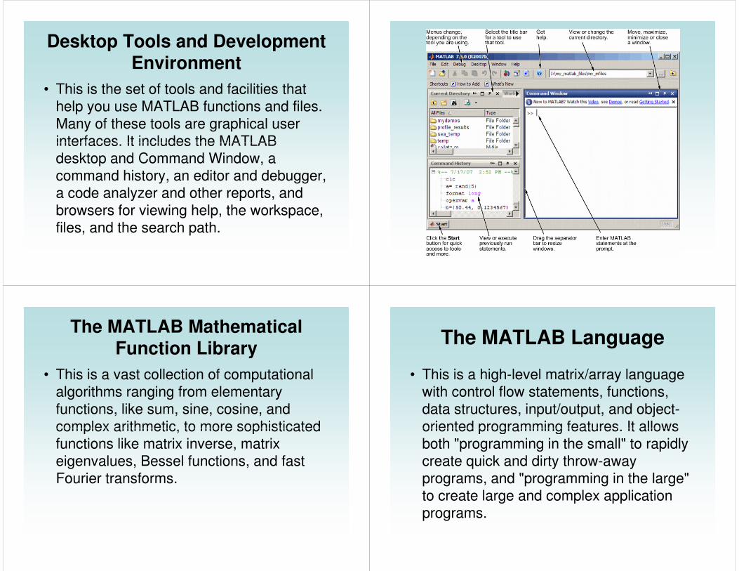
Desktop Tools and Development Environment
• This is the set of tools and facilities that help you use MATLAB functions and files. Many of these tools are graphical user interfaces. It includes the MATLAB interfaces. It includes the MATLAB desktop and Command Window, a command history, an editor and debugger, a code analyzer and other reports, and browsers for viewing help, the workspace, files, and the search path.
The MATLAB Mathematical Function Library
• This is a vast collection of computational algorithms ranging from elementary functions, like sum, sine, cosine, and complex arithmetic, to more sophisticated complex arithmetic, to more sophisticated functions like matrix inverse, matrix eigenvalues, Bessel functions, and fast Fourier transforms.
The MATLAB Language
• This is a high-level matrix/array language with control flow statements, functions, data structures, input/output, and object-oriented programming features. It allows oriented programming features. It allows both "programming in the small" to rapidly create quick and dirty throw-away programs, and "programming in the large" to create large and complex application programs.
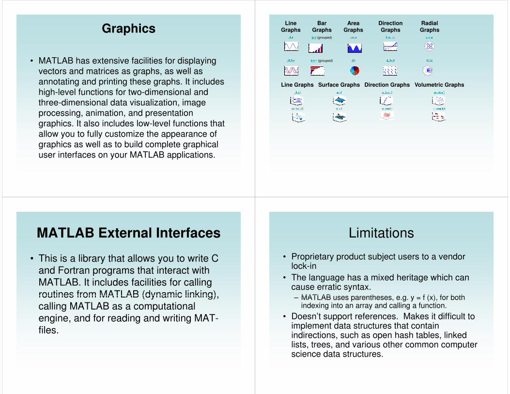
Graphics
• MATLAB has extensive facilities for displaying
vectors and matrices as graphs, as well as
annotating and printing these graphs. It includes
high-level functions for two-dimensional and
three-dimensional data visualization, image three-dimensional data visualization, image
processing, animation, and presentation
graphics. It also includes low-level functions that
allow you to fully customize the appearance of
graphics as well as to build complete graphical
user interfaces on your MATLAB applications.
Line Graphs
Bar Graphs
Area Graphs
Direction Graphs
Radial Graphsplot bar (grouped) area feather polar
plotyy barh (grouped) pie quiver roseLine Graphs Surface Graphs Direction Graphs Volumetric Graphsplot3 surf quiver3 scatter3contour3 surfl comet3 coneplot
MATLAB External Interfaces
• This is a library that allows you to write C and Fortran programs that interact with MATLAB. It includes facilities for calling routines from MATLAB (dynamic linking), routines from MATLAB (dynamic linking), calling MATLAB as a computational engine, and for reading and writing MAT-files.
Limitations
• Proprietary product subject users to a vendor lock-in
• The language has a mixed heritage which can cause erratic syntax.– MATLAB uses parentheses, e.g. y = f (x), for both – MATLAB uses parentheses, e.g. y = f (x), for both
indexing into an array and calling a function.
• Doesn’t support references. Makes it difficult to implement data structures that contain indirections, such as open hash tables, linked lists, trees, and various other common computer science data structures.
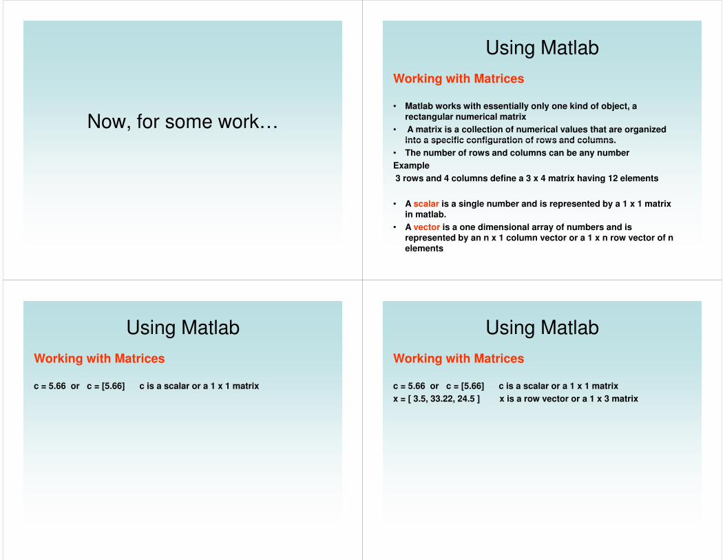
Now, for some work…
Using Matlab
Working with Matrices
• Matlab works with essentially only one kind of object, a rectangular numerical matrix
• A matrix is a collection of numerical values that are organized into a specific configuration of rows and columns. into a specific configuration of rows and columns.
• The number of rows and columns can be any number
Example
3 rows and 4 columns define a 3 x 4 matrix having 12 elements
• A scalar is a single number and is represented by a 1 x 1 matrix in matlab.
• A vector is a one dimensional array of numbers and is represented by an n x 1 column vector or a 1 x n row vector of n elements
Using Matlab
Working with Matrices
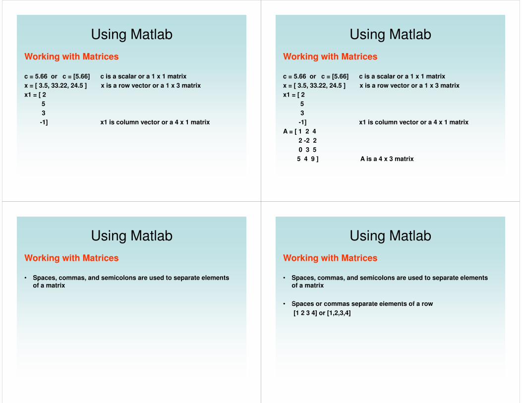
c = 5.66 or c = [5.66] c is a scalar or a 1 x 1 matrix
Using Matlab
Working with Matrices
c = 5.66 or c = [5.66] c is a scalar or a 1 x 1 matrix
x = [ 3.5, 33.22, 24.5 ] x is a row vector or a 1 x 3 matrix
Using Matlab
Working with Matrices
c = 5.66 or c = [5.66] c is a scalar or a 1 x 1 matrix
x = [ 3.5, 33.22, 24.5 ] x is a row vector or a 1 x 3 matrix
x1 = [ 2
55
3
-1] x1 is column vector or a 4 x 1 matrix
Using Matlab
Working with Matrices
c = 5.66 or c = [5.66] c is a scalar or a 1 x 1 matrix
x = [ 3.5, 33.22, 24.5 ] x is a row vector or a 1 x 3 matrix
x1 = [ 2
55
3
-1] x1 is column vector or a 4 x 1 matrix
A = [ 1 2 4
2 -2 2
0 3 5
5 4 9 ] A is a 4 x 3 matrix
Using Matlab
Working with Matrices
• Spaces, commas, and semicolons are used to separate elements of a matrix
Using Matlab
Working with Matrices
• Spaces, commas, and semicolons are used to separate elements of a matrix
• Spaces or commas separate elements of a row• Spaces or commas separate elements of a row
[1 2 3 4] or [1,2,3,4]

Using Matlab
Working with Matrices
• Spaces, commas, and semicolons are used to separate elements of a matrix
• Spaces or commas separate elements of a row• Spaces or commas separate elements of a row
[1 2 3 4] or [1,2,3,4]
• Semicolons separate columns
[1,2,3,4;5,6,7,8;9,8,7,6] = [1 2 3 4
5 6 7 8
9 8 7 6]
Using Matlab
Indexing Matrices
• A m x n matrix is defined by the number of m rows and number of n columns
• An individual element of a matrix can be specified with the notation An individual element of a matrix can be specified with the notation An individual element of a matrix can be specified with the notation An individual element of a matrix can be specified with the notation A(i,j) or Ai,j for the generalized element, or by A(4,1)=5 for a specific A(i,j) or Ai,j for the generalized element, or by A(4,1)=5 for a specific A(i,j) or Ai,j for the generalized element, or by A(4,1)=5 for a specific A(i,j) or Ai,j for the generalized element, or by A(4,1)=5 for a specific A(i,j) or Ai,j for the generalized element, or by A(4,1)=5 for a specific A(i,j) or Ai,j for the generalized element, or by A(4,1)=5 for a specific A(i,j) or Ai,j for the generalized element, or by A(4,1)=5 for a specific A(i,j) or Ai,j for the generalized element, or by A(4,1)=5 for a specific element.element.element.element.
Example:
>> A = [1 2 4 5;6 3 8 2] A is a 4 x 2 matrix
>> A(1,2)
Ans 6
• The colon operator can be used to index a range of elements
>> A(1:3,2)
Ans 1 2 4
Using Matlab
Indexing Matrices
• Specific elements of any matrix can be overwritten using the matrix index
Example:
A = [1 2 4 5A = [1 2 4 5
6 3 8 2]
>> A(1,2) = 9
Ans
A = [1 2 4 5
9 3 8 2]
Using Matlab
Matrix Shortcuts
• The ones and zeros functions can be used to create any m x n matrices composed entirely of ones or zeros
ExampleExample
a = ones(2,3)
a = [1 1
1 1
1 1]
b = zeros(1,5)
b = [0 0 0 0 0]
Using MatlabData Types and Formats
• The semicolon operator determines whether the result of an expression is displayed
• whowhowhowho lists all of the variables in your matlab workspacelists all of the variables in your matlab workspacelists all of the variables in your matlab workspacelists all of the variables in your matlab workspace
• whos list the variables and describes their matrix size
Using Matlab
Saving your WorkTo save data to a *.mat file:
Typing ‘save filename’ at the >> prompt and the file ‘filename.mat’ will be saved to the working directorySelect Save from the file pull down menu
To reload a *.mat file
1. Type ‘load filename’ at the >> prompt to load ‘filename.mat’(ensure the filename is located in the current working directory)2. Select Open from the file pull down menu and manually find the datafile
Exercises
Enter the following Matrices in matlab using spaces,
commas, and semicolons to separate rows and
columns:
9175
6211
[ ]553878122641A = B =
7231
9175 [ ]553878122641
160
16
22
4
A = B =
C =
19246525
12100
2162855
42166418
D =
[ ]65D =
E = a 5 x 9 matrix of 1’s
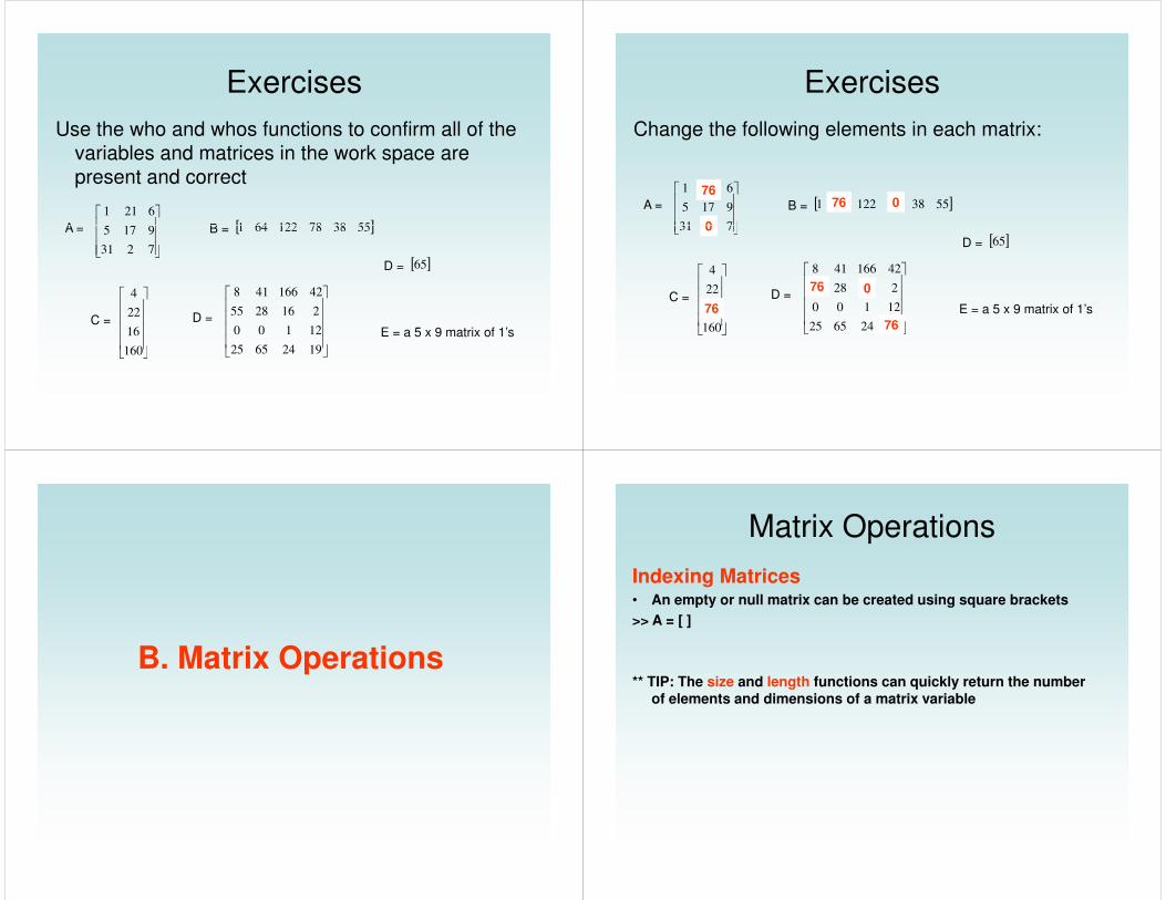
Exercises
Use the who and whos functions to confirm all of the
variables and matrices in the work space are
present and correct
9175
6211
[ ]553878122641A = B =
7231
9175 [ ]553878122641
160
16
22
4
A = B =
C =
19246525
12100
2162855
42166418
D =
[ ]65D =
E = a 5 x 9 matrix of 1’s
Exercises
Change the following elements in each matrix:
7231
9175
661
[ ]553878122641A = B =76
76 0
0 7231
160
16
22
4
C =
19246525
12100
2162855
42166418
D =
[ ]65D =
E = a 5 x 9 matrix of 1’s76
76
76
0
0
B. Matrix Operations
Indexing Matrices• An empty or null matrix can be created using square brackets
>> A = [ ]
** TIP: The size and length functions can quickly return the number
Matrix Operations
** TIP: The size and length functions can quickly return the number of elements and dimensions of a matrix variable
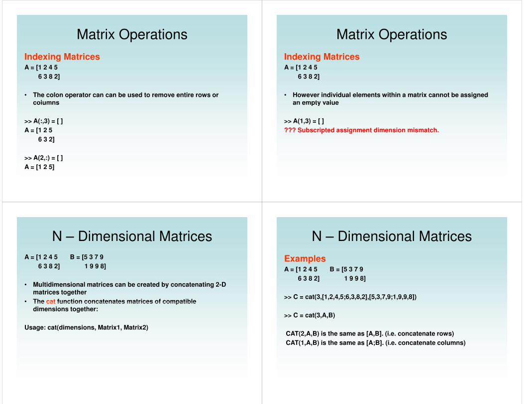
Indexing MatricesA = [1 2 4 5
6 3 8 2]
• The colon operator can can be used to remove entire rows or columns
Matrix Operations
columns
>> A(:,3) = [ ]
A = [1 2 5
6 3 2]
>> A(2,:) = [ ]
A = [1 2 5]
Indexing MatricesA = [1 2 4 5
6 3 8 2]
• However individual elements within a matrix cannot be assigned an empty value
Matrix Operations
an empty value
>> A(1,3) = [ ]
??? Subscripted assignment dimension mismatch.
A = [1 2 4 5 B = [5 3 7 9
6 3 8 2] 1 9 9 8]
• Multidimensional matrices can be created by concatenating 2-D matrices together
• The cat function concatenates matrices of compatible
N – Dimensional Matrices
• The cat function concatenates matrices of compatible dimensions together:
Usage: cat(dimensions, Matrix1, Matrix2)
ExamplesA = [1 2 4 5 B = [5 3 7 9
6 3 8 2] 1 9 9 8]
>> C = cat(3,[1,2,4,5;6,3,8,2],[5,3,7,9;1,9,9,8])
N – Dimensional Matrices
>> C = cat(3,A,B)
CAT(2,A,B) is the same as [A,B]. (i.e. concatenate rows)
CAT(1,A,B) is the same as [A;B]. (i.e. concatenate columns)
Scalar Operations• Scalar (single value) calculations can be can performed on
matrices and arrays
Basic Calculation Operators
+ Addition
Matrix Operations
+ Addition
- Subtraction
* Multiplication
/ Division
^ Exponentiation
Scalar Operations• Scalar (single value) calculations can be performed on matrices
and arrays
A = [1 2 4 5 B = [1 C = 5
6 3 8 2] 7
Matrix Operations
6 3 8 2] 7
3
3]
Try:
A + 10
A * 5
B / 2
A^C
Scalar Operations• Scalar (single value) calculations can be performed on matrices
and arrays
A = [1 2 4 5 B = [1 C = 5
6 3 8 2] 7
Matrix Operations
6 3 8 2] 7
3
3]
Try:
A + 10
A * 5
B / 2
A^C What is happening here?
Matrix Operations• Matrix to matrix calculations can be performed on matrices and
arrays
Addition and Subtraction• Matrix dimensions must be the same or the added/subtracted
value must be scalar
Matrix Operations
value must be scalar
A = [1 2 4 5 B = [1 C = 5 D = [2 4 6 8
6 3 8 2] 7 1 3 5 7]
3
3]
Try:
>>A + B >>A + C >>A + D
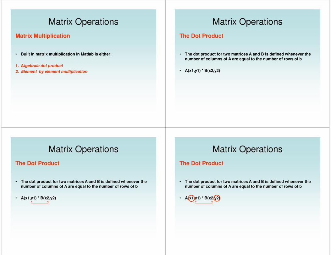
Matrix Multiplication
• Built in matrix multiplication in Matlab is either:
1. Algebraic dot product
Matrix Operations
1. Algebraic dot product
2. Element by element multiplication
The Dot Product
• The dot product for two matrices A and B is defined whenever the number of columns of A are equal to the number of rows of b
Matrix Operations
• A(x1,y1) * B(x2,y2)
The Dot Product
• The dot product for two matrices A and B is defined whenever the number of columns of A are equal to the number of rows of b
Matrix Operations
• A(x1,y1) * B(x2,y2)
The Dot Product
• The dot product for two matrices A and B is defined whenever the number of columns of A are equal to the number of rows of b
Matrix Operations
• A(x1,y1) * B(x2,y2)
The Dot Product
• The dot product for two matrices A and B is defined whenever the number of columns of A are equal to the number of rows of b
Matrix Operations
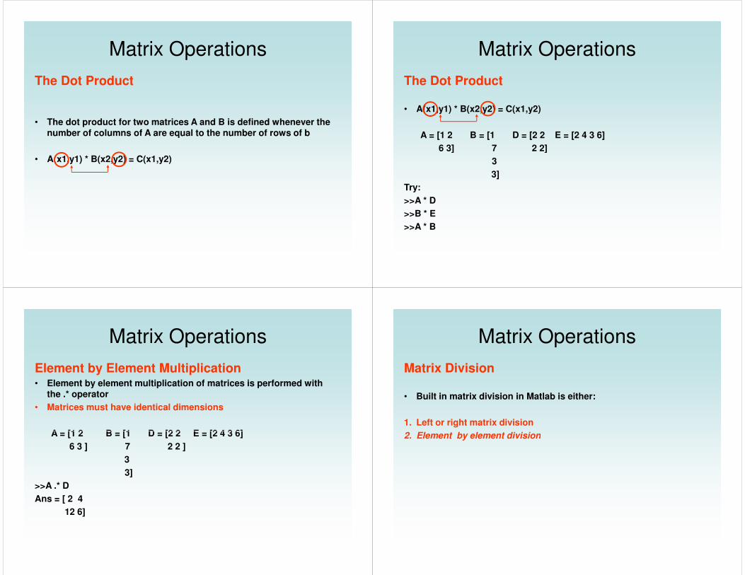
• A(x1,y1) * B(x2,y2) = C(x1,y2)
The Dot Product
• A(x1,y1) * B(x2,y2) = C(x1,y2)
A = [1 2 B = [1 D = [2 2 E = [2 4 3 6]
6 3] 7 2 2]
Matrix Operations
6 3] 7 2 2]
3
3]
Try:
>>A * D
>>B * E
>>A * B
Element by Element Multiplication• Element by element multiplication of matrices is performed with
the .* operator
• Matrices must have identical dimensions
A = [1 2 B = [1 D = [2 2 E = [2 4 3 6]
Matrix Operations
A = [1 2 B = [1 D = [2 2 E = [2 4 3 6]
6 3 ] 7 2 2 ]
3
3]
>>A .* D
Ans = [ 2 4
12 6]
Matrix Division
• Built in matrix division in Matlab is either:
1. Left or right matrix division
2. Element by element division
Matrix Operations
2. Element by element division
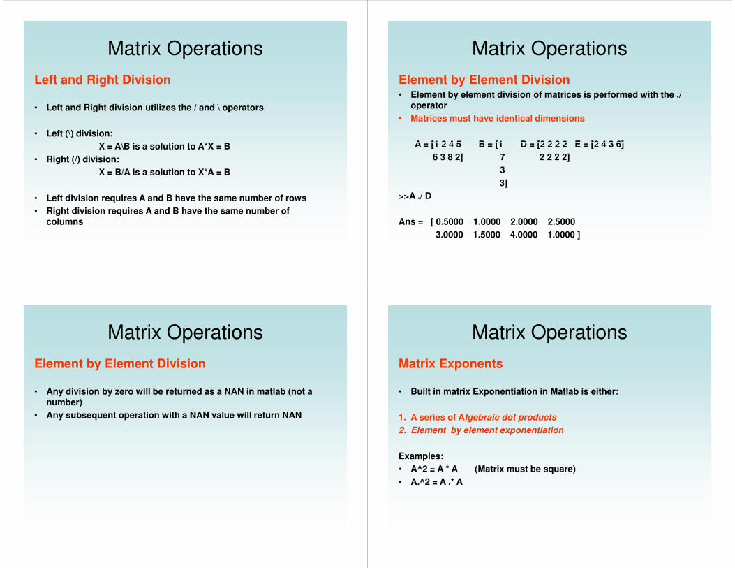
Left and Right Division
• Left and Right division utilizes the / and \ operators
• Left (\) division:
X = A\B is a solution to A*X = B
Matrix Operations
X = A\B is a solution to A*X = B
• Right (/) division:
X = B/A is a solution to X*A = B
• Left division requires A and B have the same number of rows
• Right division requires A and B have the same number of columns
Element by Element Division• Element by element division of matrices is performed with the ./
operator
• Matrices must have identical dimensions
A = [1 2 4 5 B = [1 D = [2 2 2 2 E = [2 4 3 6]
Matrix Operations
A = [1 2 4 5 B = [1 D = [2 2 2 2 E = [2 4 3 6]
6 3 8 2] 7 2 2 2 2]
3
3]
>>A ./ D
Ans = [ 0.5000 1.0000 2.0000 2.5000
3.0000 1.5000 4.0000 1.0000 ]
Element by Element Division
• Any division by zero will be returned as a NAN in matlab (not a number)
• Any subsequent operation with a NAN value will return NAN
Matrix Operations
Matrix Exponents
• Built in matrix Exponentiation in Matlab is either:
1. A series of Algebraic dot products
2. Element by element exponentiation
Matrix Operations
2. Element by element exponentiation
Examples:
• A^2 = A * A (Matrix must be square)
• A.^2 = A .* A
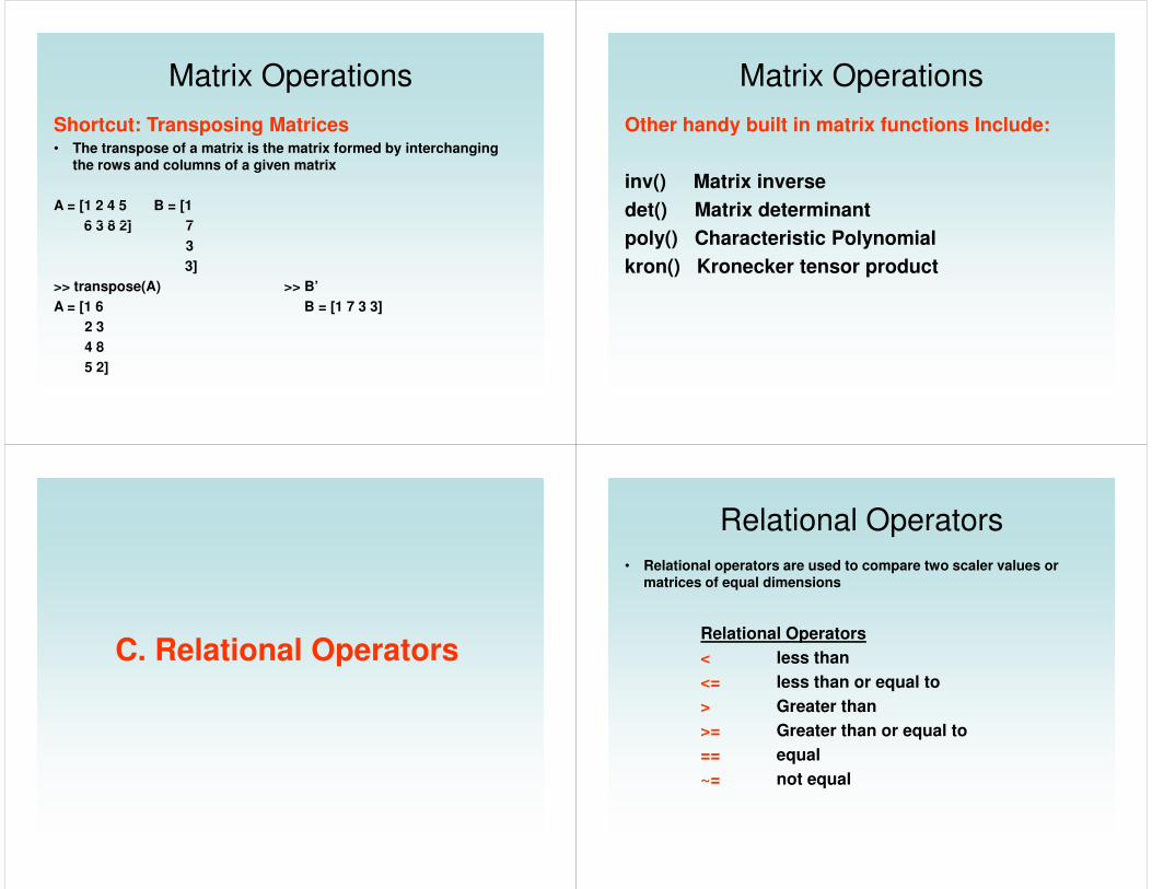
Shortcut: Transposing Matrices• The transpose of a matrix is the matrix formed by interchanging
the rows and columns of a given matrix
A = [1 2 4 5 B = [1
6 3 8 2] 7
Matrix Operations
6 3 8 2] 7
3
3]
>> transpose(A) >> B’
A = [1 6 B = [1 7 3 3]
2 3
4 8
5 2]
Other handy built in matrix functions Include:
inv() Matrix inverse
det() Matrix determinant
Matrix Operations
poly() Characteristic Polynomial
kron() Kronecker tensor product
C. Relational Operators
• Relational operators are used to compare two scaler values or matrices of equal dimensions
Relational Operators
< less than
Relational Operators
<= less than or equal to
> Greater than
>= Greater than or equal to
== equal
~= not equal
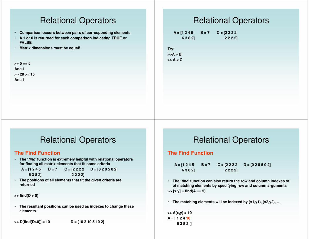
• Comparison occurs between pairs of corresponding elements
• A 1 or 0 is returned for each comparison indicating TRUE or FALSE
• Matrix dimensions must be equal!
Relational Operators
>> 5 == 5
Ans 1
>> 20 >= 15
Ans 1
A = [1 2 4 5 B = 7 C = [2 2 2 2
6 3 8 2] 2 2 2 2]
Try:
>>A > B
>> A < C
Relational Operators
>> A < C
The Find Function• The ‘find’ function is extremely helpful with relational operators
for finding all matrix elements that fit some criteria
A = [1 2 4 5 B = 7 C = [2 2 2 2 D = [0 2 0 5 0 2]
6 3 8 2] 2 2 2 2]
• The positions of all elements that fit the given criteria are
Relational Operators
• The positions of all elements that fit the given criteria are returned
>> find(D > 0)
• The resultant positions can be used as indexes to change these elements
>> D(find(D>0)) = 10 D = [10 2 10 5 10 2]
The Find Function
A = [1 2 4 5 B = 7 C = [2 2 2 2 D = [0 2 0 5 0 2]
6 3 8 2] 2 2 2 2]
• The ‘find’ function can also return the row and column indexes of
Relational Operators
• The ‘find’ function can also return the row and column indexes of of matching elements by specifying row and column arguments
>> [x,y] = find(A == 5)
• The matching elements will be indexed by (x1,y1), (x2,y2), …
>> A(x,y) = 10
A = [ 1 2 4 10
6 3 8 2 ]
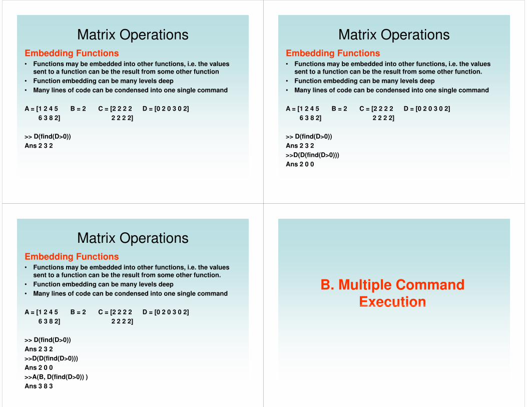
Embedding Functions• Functions may be embedded into other functions, i.e. the values
sent to a function can be the result from some other function
• Function embedding can be many levels deep
• Many lines of code can be condensed into one single command
Matrix Operations
A = [1 2 4 5 B = 2 C = [2 2 2 2 D = [0 2 0 3 0 2]
6 3 8 2] 2 2 2 2]
>> D(find(D>0))
Ans 2 3 2
Embedding Functions• Functions may be embedded into other functions, i.e. the values
sent to a function can be the result from some other function.
• Function embedding can be many levels deep
• Many lines of code can be condensed into one single command
Matrix Operations
A = [1 2 4 5 B = 2 C = [2 2 2 2 D = [0 2 0 3 0 2]
6 3 8 2] 2 2 2 2]
>> D(find(D>0))
Ans 2 3 2
>>D(D(find(D>0)))
Ans 2 0 0
>>A(B, D(find(D>0)) )
Ans 3 8 3
B. Multiple Command ExecutionExecution
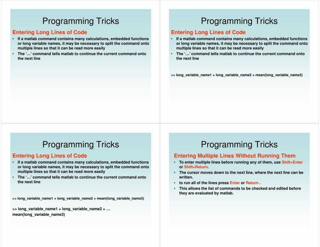
Entering Long Lines of Code• If a matlab command contains many calculations, embedded functions
or long variable names, it may be necessary to split the command onto multiple lines so that it can be read more easily
• The ‘…’ command tells matlab to continue the current command onto the next line
Programming TricksEntering Long Lines of Code• If a matlab command contains many calculations, embedded functions
or long variable names, it may be necessary to split the command onto multiple lines so that it can be read more easily
• The ‘…’ command tells matlab to continue the current command onto the next line
Programming Tricks
>> long_variable_name1 + long_variable_name2 + mean(long_variable_name3)
Entering Long Lines of Code• If a matlab command contains many calculations, embedded functions
or long variable names, it may be necessary to split the command onto multiple lines so that it can be read more easily
• The ‘…’ command tells matlab to continue the current command onto the next line
Programming Tricks
>> long_variable_name1 + long_variable_name2 + mean(long_variable_name3)
>> long_variable_name1 + long_variable_name2 + …
mean(long_variable_name3)
Entering Multiple Lines Without Running Them• To enter multiple lines before running any of them, use Shift+Enter
or Shift+Return.
• The cursor moves down to the next line, where the next line can be written.
• to run all of the lines press Enter or Return .
Programming Tricks
• This allows the list of commands to be checked and edited before they are evaluated by matlab.
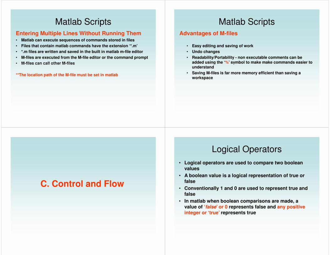
Entering Multiple Lines Without Running Them• Matlab can execute sequences of commands stored in files
• Files that contain matlab commands have the extension ‘*.m’
• *.m files are written and saved in the built in matlab m-file editor
• M-files are executed from the M-file editor or the command prompt
• M-files can call other M-files
Matlab Scripts
• M-files can call other M-files
**The location path of the M-file must be set in matlab
Advantages of M-files
• Easy editing and saving of work
• Undo changes
• Readability/Portability - non executable comments can be added using the ‘%’ symbol to make make commands easier to
Matlab Scripts
added using the ‘%’ symbol to make make commands easier to understand
• Saving M-files is far more memory efficient than saving a workspace
C. Control and Flow
• Logical operators are used to compare two boolean values
• A boolean value is a logical representation of true or false
• Conventionally 1 and 0 are used to represent true and false
Logical Operators
false
• In matlab when boolean comparisons are made, a value of ‘false’ or 0 represents false and any positive integer or ‘true’ represents true
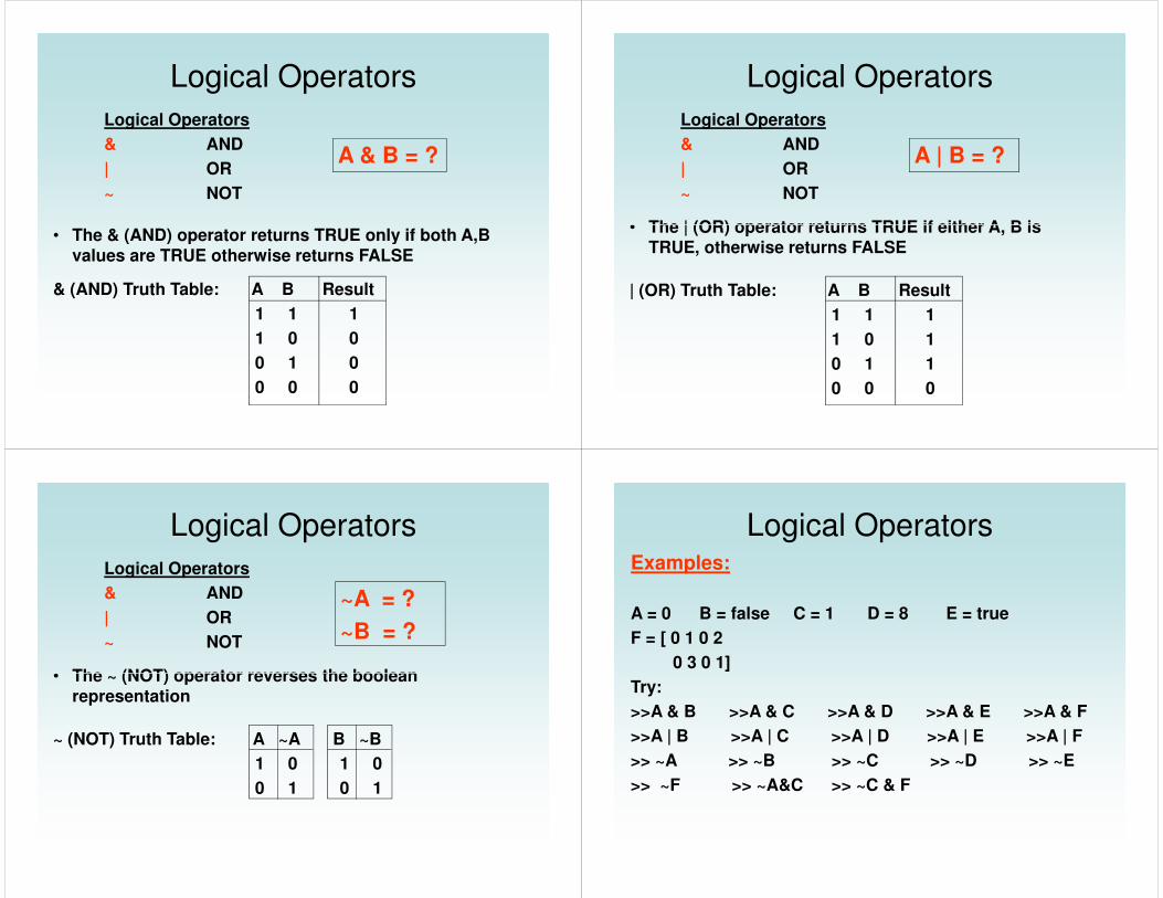
Logical Operators
& AND
| OR
~ NOT
The & (AND) operator returns TRUE only if both A,B
Logical Operators
A & B = ?
• The & (AND) operator returns TRUE only if both A,B values are TRUE otherwise returns FALSE
& (AND) Truth Table: A B Result
1 1 1
1 0 0
0 1 0
0 0 0
Logical Operators
& AND
| OR
~ NOT
• The | (OR) operator returns TRUE if either A, B is
Logical Operators
A | B = ?
• The | (OR) operator returns TRUE if either A, B is TRUE, otherwise returns FALSE
| (OR) Truth Table: A B Result
1 1 1
1 0 1
0 1 1
0 0 0
Logical Operators
& AND
| OR
~ NOT
• The ~ (NOT) operator reverses the boolean
Logical Operators
~A = ?
~B = ?
• The ~ (NOT) operator reverses the boolean representation
~ (NOT) Truth Table: A ~A B ~B
1 0 1 0
0 1 0 1
Examples:
A = 0 B = false C = 1 D = 8 E = true
F = [ 0 1 0 2
0 3 0 1]
Logical Operators
Try:
>>A & B >>A & C >>A & D >>A & E >>A & F
>>A | B >>A | C >>A | D >>A | E >>A | F
>> ~A >> ~B >> ~C >> ~D >> ~E
>> ~F >> ~A&C >> ~C & F
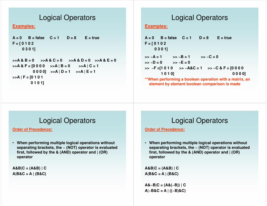
Examples:
A = 0 B = false C = 1 D = 8 E = true
F = [ 0 1 0 2
0 3 0 1]
Logical Operators
>>A & B = 0 >>A & C = 0 >>A & D = 0 >>A & E = 0
>>A & F = [0 0 0 0 >>A | B = 0 >>A | C = 1
0 0 0 0] >>A | D = 1 >>A | E = 1
>>A | F = [0 1 0 1
0 1 0 1]
Examples:
A = 0 B = false C = 1 D = 8 E = true
F = [ 0 1 0 2
0 3 0 1]
Logical Operators
>> ~A = 1 >> ~B = 1 >> ~C = 0
>> ~D = 0 >> ~E = 0
>> ~F =[1 0 1 0 >> ~A&C = 1 >> ~C & F = [0 0 0 0
1 0 1 0] 0 0 0 0]
**When performing a boolean operation with a matrix, an element by element boolean comparison is made
Order of Precedence:
• When performing multiple logical operations without separating brackets, the ~ (NOT) operator is evaluated first, followed by the & (AND) operator and | (OR) operator
Logical Operators
operator
A&B|C = (A&B) | C
A|B&C = A | (B&C)
Order of Precedence:
• When performing multiple logical operations without separating brackets, the ~ (NOT) operator is evaluated first, followed by the & (AND) operator and | (OR) operator
Logical Operators
operator
A&B|C = (A&B) | C
A|B&C = A | (B&C)
A&~B|C = (A&(~B)) | C
A|~B&C = A | ((~B)&C)
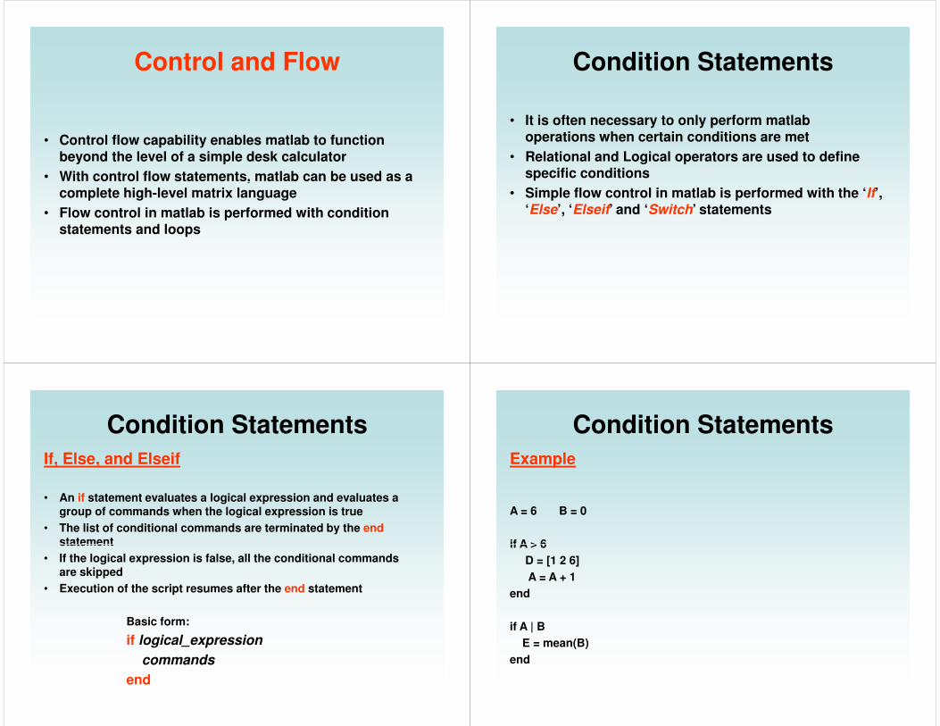
• Control flow capability enables matlab to function beyond the level of a simple desk calculator
• With control flow statements, matlab can be used as a
Control and Flow
• With control flow statements, matlab can be used as a complete high-level matrix language
• Flow control in matlab is performed with condition statements and loops
• It is often necessary to only perform matlab operations when certain conditions are met
• Relational and Logical operators are used to define specific conditions
Condition Statements
• Simple flow control in matlab is performed with the ‘If’, ‘Else’, ‘Elseif’ and ‘Switch’ statements
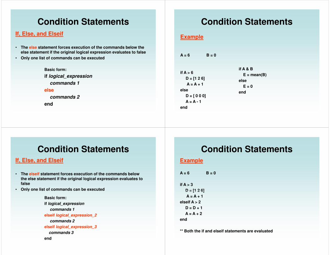
If, Else, and Elseif
• An if statement evaluates a logical expression and evaluates a group of commands when the logical expression is true
• The list of conditional commands are terminated by the end statement
Condition Statements
statement
• If the logical expression is false, all the conditional commands are skipped
• Execution of the script resumes after the end statement
Basic form:
if logical_expression
commands
end
Example
A = 6 B = 0
if A > 6
Condition Statements
if A > 6
D = [1 2 6]
A = A + 1
end
if A | B
E = mean(B)
end
If, Else, and Elseif
• The else statement forces execution of the commands below the else statement if the original logical expression evaluates to false
• Only one list of commands can be executed
Condition Statements
Basic form:
if logical_expression
commands 1
else
commands 2
end
Example
A = 6 B = 0
Condition Statements
if A > 6
D = [1 2 6]
A = A + 1
else
D = [ 0 0 0]
A = A - 1
end
if A & B
E = mean(B)
else
E = 0
end
If, Else, and Elseif
• The elseif statement forces execution of the commands below the else statement if the original logical expression evaluates to false
• Only one list of commands can be executed
Condition Statements
• Only one list of commands can be executed
Basic form:
if logical_expression
commands 1
elseif logical_expression_2
commands 2
elseif logical_expression_3
commands 3
end
Example
A = 6 B = 0
if A > 3
D = [1 2 6]
Condition Statements
D = [1 2 6]
A = A + 1
elseif A > 2
D = D + 1
A = A + 2
end
** Both the if and elseif statements are evaluated
Switch• The switch statement can act as many elseif statements
• Only the one case statement who’s value satisfies the original expression is evaluated
Basic form:
switch expression (scalar or string)
Condition Statements
switch expression (scalar or string)
case value 1
commands 1
case value 2
commands 2
case value n
commands n
end
Example
A = 6 B = 0
switch A
case 4
D = [ 0 0 0]
A = A - 1
Condition Statements
A = A - 1
case 5
B = 1
case 6
D = [1 2 6]
A = A + 1
end
** Only case 6 is evaluated
• Loops are an important component of flow control that enables matlab to repeat multiple statements in specific and controllable ways
Loops
• Simple repetition in matlab is controlled by two types of loops:
1. For loops
2. While loops
For Loops
• The for loop executes a statement or group of statements a predetermined number of times
Loops
Basic Form:
for index = start:increment:end
statements
end
** If ‘increment’ is not specified, an increment of 1 is assumed by matlab
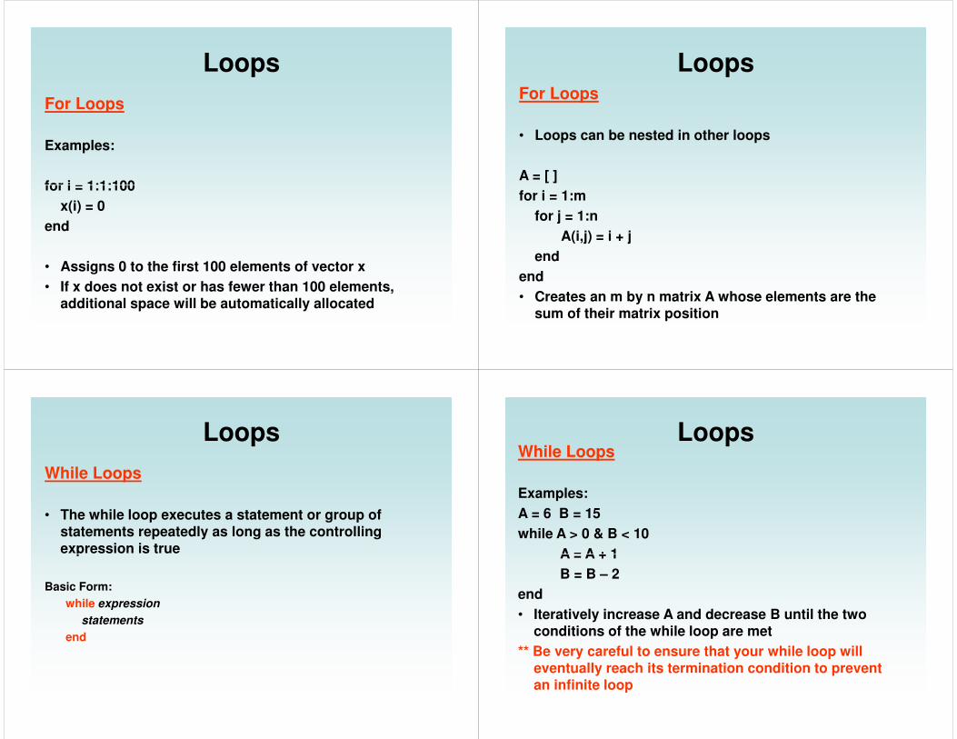
For Loops
Examples:
for i = 1:1:100
Loops
for i = 1:1:100
x(i) = 0
end
• Assigns 0 to the first 100 elements of vector x
• If x does not exist or has fewer than 100 elements, additional space will be automatically allocated
For Loops
• Loops can be nested in other loops
A = [ ]
Loops
for i = 1:m
for j = 1:n
A(i,j) = i + j
end
end
• Creates an m by n matrix A whose elements are the sum of their matrix position
While Loops
• The while loop executes a statement or group of statements repeatedly as long as the controlling expression is true
Loops
expression is true
Basic Form:
while expression
statements
end
While Loops
Examples:
A = 6 B = 15
while A > 0 & B < 10
A = A + 1
Loops
A = A + 1
B = B – 2
end
• Iteratively increase A and decrease B until the two conditions of the while loop are met
** Be very careful to ensure that your while loop will eventually reach its termination condition to prevent an infinite loop
While Loops
Examples:
A = 6 B = 15
while A > 0 & B < 10
if A < 0
Loops
if A < 0
A = A + 1
elseif B > 10
B = B – 2
end
end
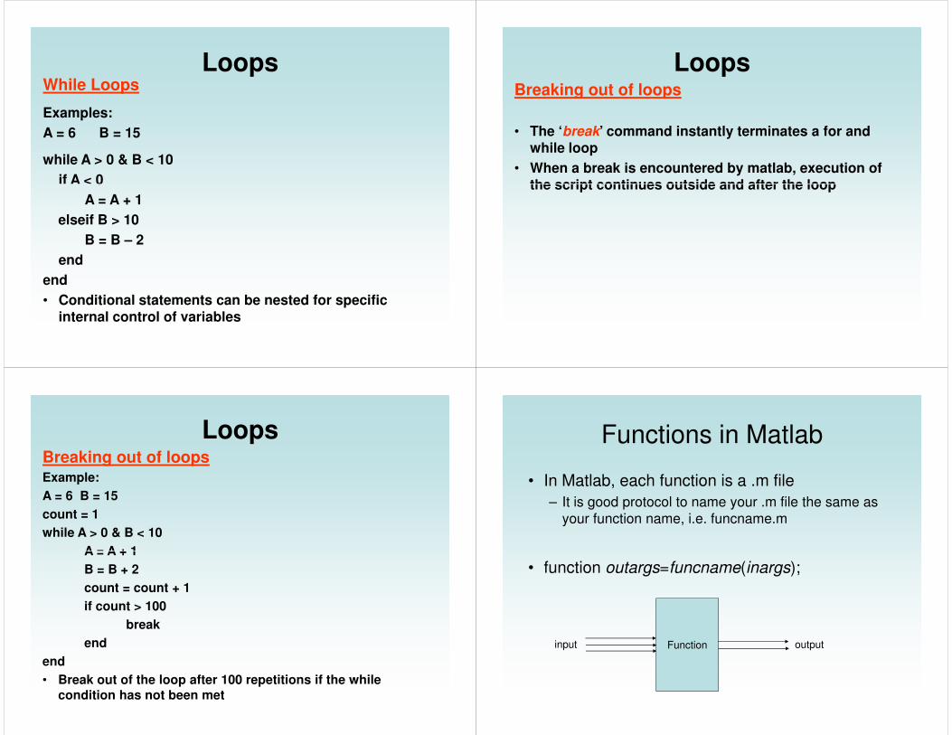
• Conditional statements can be nested for specific internal control of variables
Breaking out of loops
• The ‘break’ command instantly terminates a for and while loop
• When a break is encountered by matlab, execution of the script continues outside and after the loop
Loops
the script continues outside and after the loop
Breaking out of loopsExample:
A = 6 B = 15
count = 1
while A > 0 & B < 10
A = A + 1
Loops
A = A + 1
B = B + 2
count = count + 1
if count > 100
break
end
end
• Break out of the loop after 100 repetitions if the while condition has not been met
Functions in Matlab
• In Matlab, each function is a .m file
– It is good protocol to name your .m file the same as
your function name, i.e. funcname.m
• function outargs=funcname(inargs);
Function outputinput
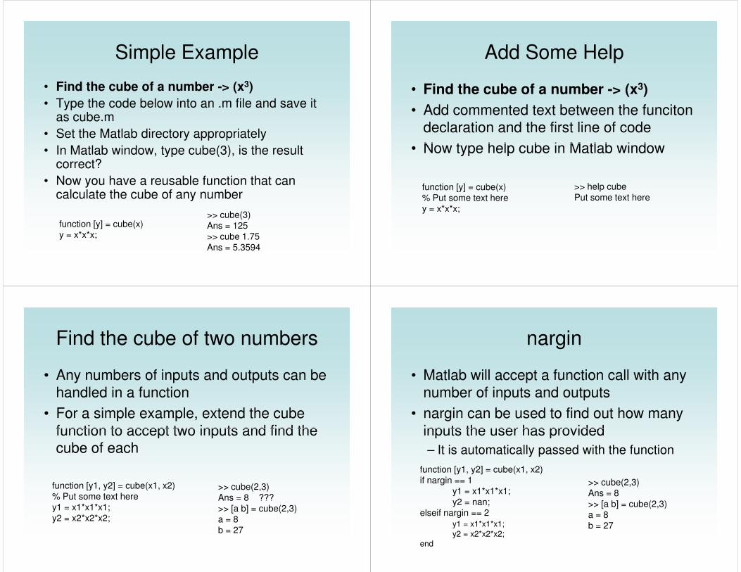
Simple Example
• Find the cube of a number -> (x3)
• Type the code below into an .m file and save it as cube.m
• Set the Matlab directory appropriately
• In Matlab window, type cube(3), is the result • In Matlab window, type cube(3), is the result correct?
• Now you have a reusable function that can calculate the cube of any number
function [y] = cube(x)y = x*x*x;
>> cube(3)Ans = 125>> cube 1.75Ans = 5.3594
Add Some Help
• Find the cube of a number -> (x3)
• Add commented text between the funciton declaration and the first line of code
• Now type help cube in Matlab window• Now type help cube in Matlab window
function [y] = cube(x)% Put some text herey = x*x*x;
>> help cubePut some text here
Find the cube of two numbers
• Any numbers of inputs and outputs can be handled in a function
• For a simple example, extend the cube function to accept two inputs and find the function to accept two inputs and find the cube of each
function [y1, y2] = cube(x1, x2)% Put some text herey1 = x1*x1*x1;y2 = x2*x2*x2;
>> cube(2,3)Ans = 8 ???>> [a b] = cube(2,3)a = 8b = 27
nargin
• Matlab will accept a function call with any number of inputs and outputs
• nargin can be used to find out how many inputs the user has providedinputs the user has provided
– It is automatically passed with the function
function [y1, y2] = cube(x1, x2)if nargin == 1
y1 = x1*x1*x1;y2 = nan;
elseif nargin == 2y1 = x1*x1*x1;
y2 = x2*x2*x2;
end
>> cube(2,3)Ans = 8>> [a b] = cube(2,3)a = 8b = 27
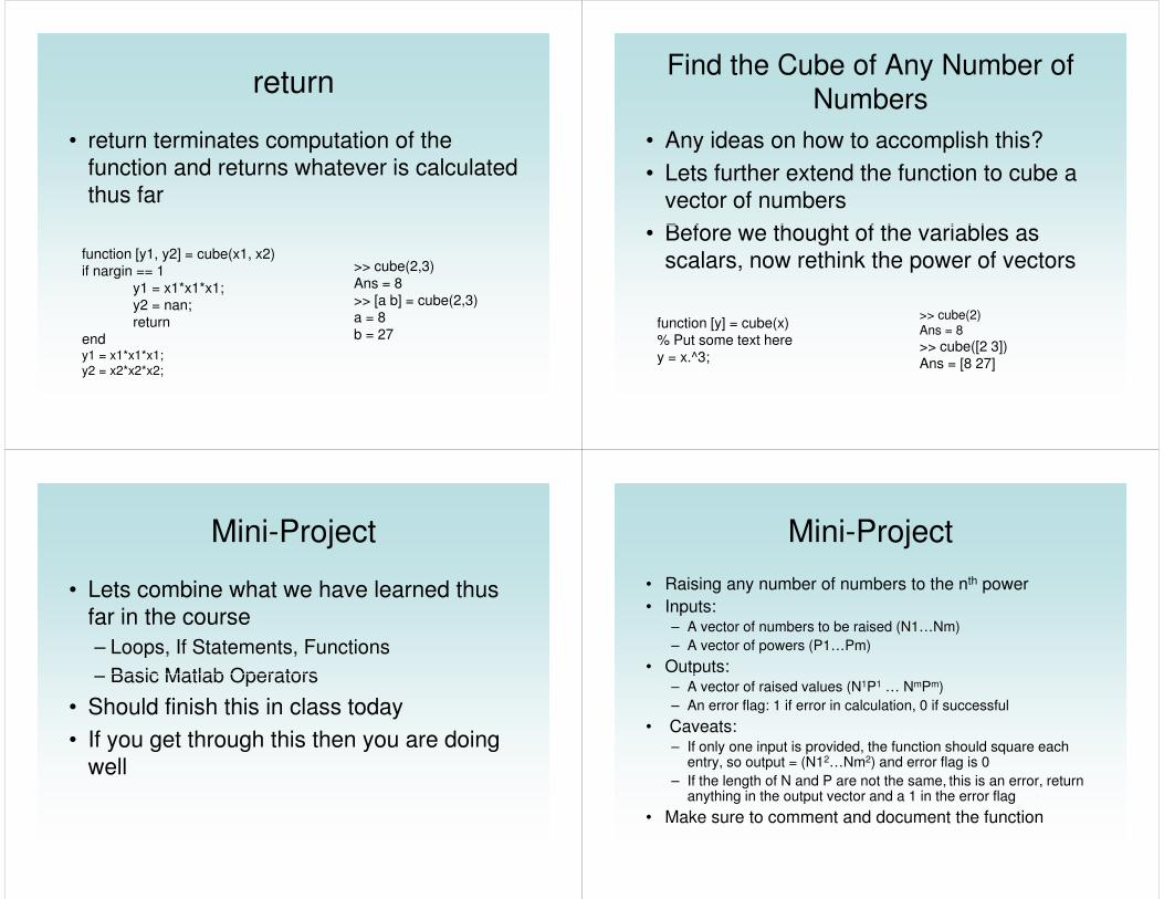
return
• return terminates computation of the function and returns whatever is calculated thus far
function [y1, y2] = cube(x1, x2)if nargin == 1
y1 = x1*x1*x1;y2 = nan;return
endy1 = x1*x1*x1;
y2 = x2*x2*x2;
>> cube(2,3)Ans = 8>> [a b] = cube(2,3)a = 8b = 27
Find the Cube of Any Number of
Numbers
• Any ideas on how to accomplish this?
• Lets further extend the function to cube a vector of numbers
• Before we thought of the variables as • Before we thought of the variables as scalars, now rethink the power of vectors
function [y] = cube(x)% Put some text herey = x.^3;
>> cube(2)
Ans = 8
>> cube([2 3])Ans = [8 27]
Mini-Project
• Lets combine what we have learned thus far in the course
– Loops, If Statements, Functions
– Basic Matlab Operators– Basic Matlab Operators
• Should finish this in class today
• If you get through this then you are doing well
Mini-Project
• Raising any number of numbers to the nth power
• Inputs:– A vector of numbers to be raised (N1…Nm)
– A vector of powers (P1…Pm)
• Outputs:• Outputs:– A vector of raised values (N1P1 … NmPm)
– An error flag: 1 if error in calculation, 0 if successful
• Caveats:– If only one input is provided, the function should square each
entry, so output = (N12…Nm2) and error flag is 0
– If the length of N and P are not the same, this is an error, return anything in the output vector and a 1 in the error flag
• Make sure to comment and document the function
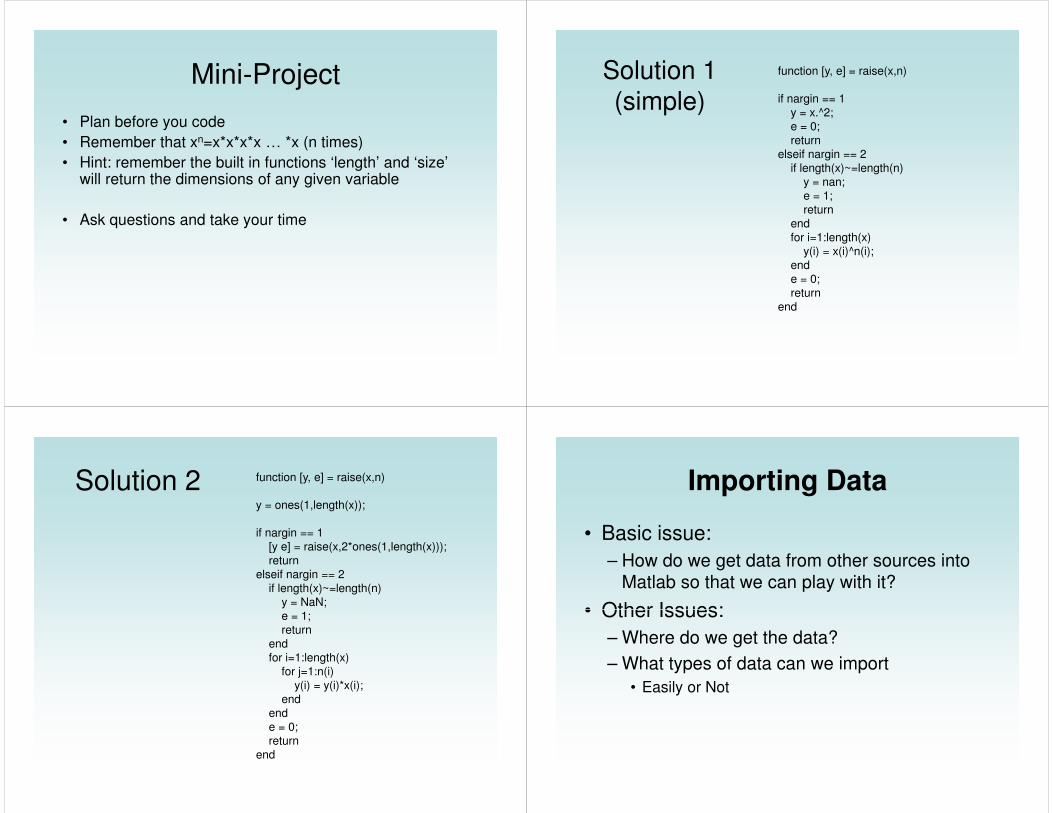
Mini-Project
• Plan before you code
• Remember that xn=x*x*x*x … *x (n times)
• Hint: remember the built in functions ‘length’ and ‘size’ will return the dimensions of any given variable
• Ask questions and take your time
Solution 1
(simple)
function [y, e] = raise(x,n)
if nargin == 1
y = x.^2;
e = 0;
return
elseif nargin == 2
if length(x)~=length(n)
y = nan;
e = 1;
returnreturn
end
for i=1:length(x)
y(i) = x(i)^n(i);
end
e = 0;
return
end
Solution 2 function [y, e] = raise(x,n)
y = ones(1,length(x));
if nargin == 1
[y e] = raise(x,2*ones(1,length(x)));
return
elseif nargin == 2
if length(x)~=length(n)
y = NaN;
e = 1;e = 1;
return
end
for i=1:length(x)
for j=1:n(i)
y(i) = y(i)*x(i);
end
end
e = 0;
return
end
Importing Data
• Basic issue:
– How do we get data from other sources into
Matlab so that we can play with it?
• Other Issues:• Other Issues:
– Where do we get the data?
– What types of data can we import
• Easily or Not
load
• Command opens and imports data from a standard ASCII file into a matlab variable
• Restrictions
– Data must be constantly sized– Data must be constantly sized
– Data must be ASCII
– No other characters
load
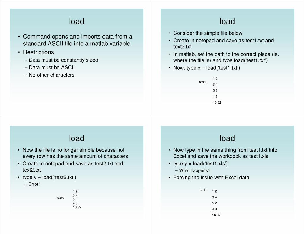
• Consider the simple file below
• Create in notepad and save as test1.txt and
text2.txt
• In matlab, set the path to the correct place (ie.
where the file is) and type load(‘test1.txt’)where the file is) and type load(‘test1.txt’)
• Now, type x = load(‘test1.txt’)
1 2
3 4
5 2
4 8
16 32
test1
load
• Now the file is no longer simple because not
every row has the same amount of characters
• Create in notepad and save as test2.txt and
text2.txt
• type y = load(‘test2.txt’)• type y = load(‘test2.txt’)
– Error!
1 2
3 4
5
4 8
16 32
test2
load
• Now type in the same thing from test1.txt into
Excel and save the workbook as test1.xls
• type y = load(‘test1.xls’)
– What happens?
• Forcing the issue with Excel data• Forcing the issue with Excel data
test11 2
3 4
5 2
4 8
16 32
load
• Works for simple and unstructured code
• Powerful and easy to use but limited
• Will likely force you to manually handle
simplifying data which is prone to error
• More complex functions are more flexible
File Handling
• f* functions are associated with file opening,
reading, manipulating, writing, …
• Basic Functions of Interest for opening and
reading generic files in matlab
– fopen– fopen
– fclose
– fseek/ftell/frewind
– fscanf
– fgetl
fopen
• Opens a file object in matlab that points to the file of interest
• fid = fopen(‘filepath’)– absolute directory + filename
• If file of interest is C:\Andrew\Project_1\file.dat• If file of interest is C:\Andrew\Project_1\file.dat
• fid = fopen(‘C:\Andrew\Project_1\file.dat’)
– relative path + filename• If your matlab path is set to c:\Andrew\Project_1
• fid = fopen(‘file.dat’)
• fid is an integer that represents the file– Can open multiple files and matlab will assign unique
fids
fclose
• When you are done with a file, it is a good idea
to close it especially if you are opening many
files
• fclose(fid)
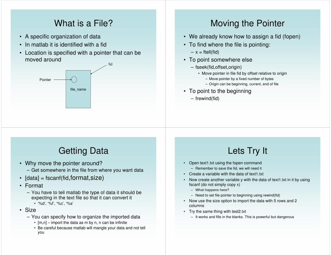
What is a File?
• A specific organization of data
• In matlab it is identified with a fid
• Location is specified with a pointer that can be
moved aroundfid
file_name
fid
Pointer
Moving the Pointer
• We already know how to assign a fid (fopen)
• To find where the file is pointing:
– x = ftell(fid)
• To point somewhere else
– fseek(fid,offset,origin)
• Move pointer in file fid by offset relative to origin
– Move pointer by a fixed number of bytes
– Origin can be beginning, current, end of file
• To point to the beginning
– frewind(fid)
Getting Data
• Why move the pointer around?– Get somewhere in the file from where you want data
• [data] = fscanf(fid,format,size)• Format
– You have to tell matlab the type of data it should be – You have to tell matlab the type of data it should be expecting in the text file so that it can convert it
• ‘%d’, ‘%f’, ‘%c’, ‘%s’
• Size– You can specify how to organize the imported data
• [m,n] – import the data as m by n, n can be infinite
• Be careful because matlab will mangle your data and not tell you
Lets Try It• Open text1.txt using the fopen command
– Remember to save the fid, we will need it
• Create a variable with the data of text1.txt
• Now create another variable y with the data of text1.txt in it by using fscanf (do not simply copy x)
– What happens here?– What happens here?
– Need to set file pointer to beginning using rewind(fid)
• Now use the size option to import the data with 5 rows and 2 columns
• Try the same thing with test2.txt
– It works and fills in the blanks. This is powerful but dangerous
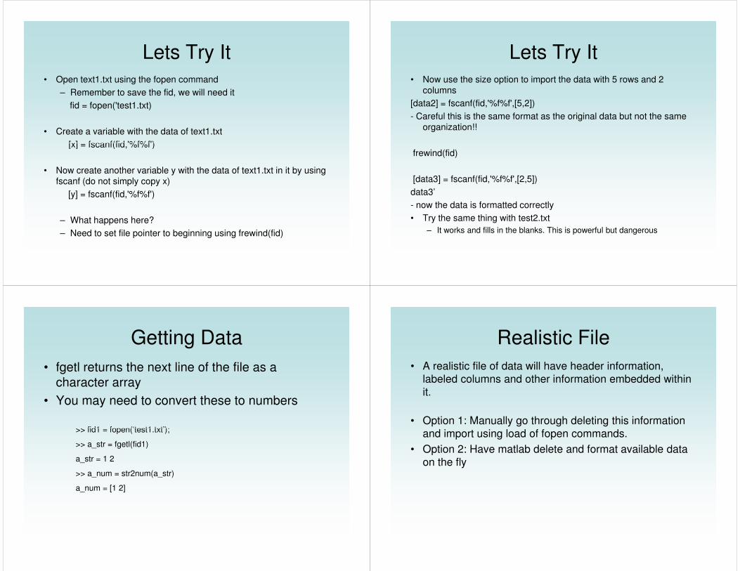
Lets Try It• Open text1.txt using the fopen command
– Remember to save the fid, we will need it
fid = fopen('test1.txt)
• Create a variable with the data of text1.txt
[x] = fscanf(fid,'%f%f')[x] = fscanf(fid,'%f%f')
• Now create another variable y with the data of text1.txt in it by using fscanf (do not simply copy x)
[y] = fscanf(fid,'%f%f')
– What happens here?
– Need to set file pointer to beginning using frewind(fid)
Lets Try It• Now use the size option to import the data with 5 rows and 2
columns
[data2] = fscanf(fid,'%f%f',[5,2])
- Careful this is the same format as the original data but not the same organization!!
frewind(fid)
[data3] = fscanf(fid,'%f%f',[2,5])
data3’
- now the data is formatted correctly
• Try the same thing with test2.txt
– It works and fills in the blanks. This is powerful but dangerous
Getting Data
• fgetl returns the next line of the file as a
character array
• You may need to convert these to numbers
>> fid1 = fopen(‘test1.txt’);>> fid1 = fopen(‘test1.txt’);
>> a_str = fgetl(fid1)
a_str = 1 2
>> a_num = str2num(a_str)
a_num = [1 2]
Realistic File
• A realistic file of data will have header information,
labeled columns and other information embedded within
it.
• Option 1: Manually go through deleting this information
and import using load of fopen commands.and import using load of fopen commands.
• Option 2: Have matlab delete and format available data
on the fly
Realistic File
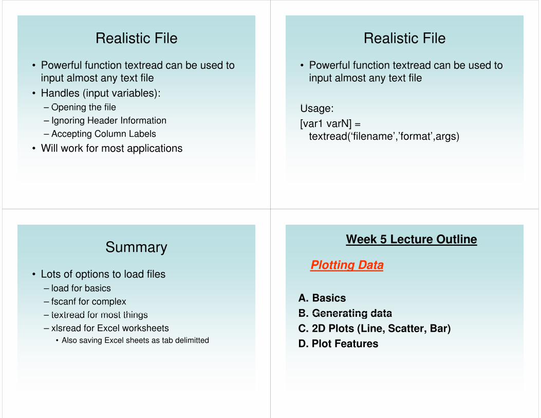
• Powerful function textread can be used to input almost any text file
• Handles (input variables):
– Opening the file– Opening the file
– Ignoring Header Information
– Accepting Column Labels
• Will work for most applications
Realistic File
• Powerful function textread can be used to input almost any text file
Usage:Usage:
[var1 varN] = textread(‘filename’,’format’,args)
Summary
• Lots of options to load files
– load for basics
– fscanf for complex
– textread for most things– textread for most things
– xlsread for Excel worksheets
• Also saving Excel sheets as tab delimitted
Week 5 Lecture Outline
Plotting Data
A. Basics
B. Generating dataB. Generating data
C. 2D Plots (Line, Scatter, Bar)
D. Plot Features
Basics• Matlab has a powerful plotting engine that can
generate a wide variety of plots.
Generating Data• Matlab does not understand functions, it can
only use arrays of numbers.
– a=t2
– b=sin(2*pi*t)
– c=e-10*t note: matlab command is exp()– c=e-10*t note: matlab command is exp()
– d=cos(4*pi*t)
– e=2t3-4t2+t
• Generate it numerically over specific range
• Try and generate a-e over the interval 0:0.01:2
t=0:0.01:10; %make x vector
y=t.^2; %now we have the appropriate y
% but only over the specified range
Line/Scatter
• Simplest plot function is plot()
• Try typing plot(y)– Matlab automatically generates a figure and draws the data and
connects its lines
– Looks right, but the x axis units are incorrect
• Type plot(x,y), will look identical but have correct x-axis • Type plot(x,y), will look identical but have correct x-axis units
• Plot(x1,y1,s1,x2,y2,s2, …) many plots in one command
• Plot(x) where x is a matrix, will result in plotting each column as a separate trace
Line/Scatter
• Plot a and then plot b
– What do you see?
– Only b
• Matlab will replace the current plot with any new one
unless you specifically tell it not tounless you specifically tell it not to
• To have both plots on one figure use the hold on
command
• To make multiple plots use the figure command
plot(t,a)
plot(t,b)
% Put a and b on one plot
plot(t,a);
hold on;
plot(t,b);
% Make two plots
plot(t,a);
figure;
plot(t,b);
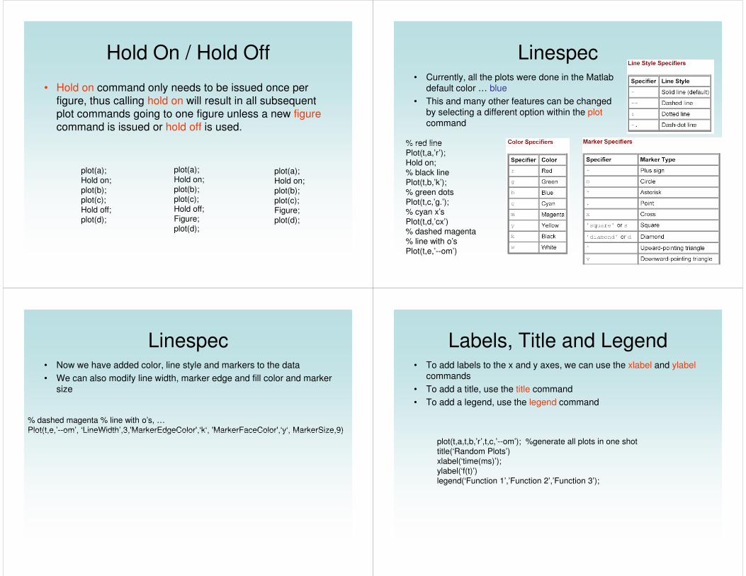
Hold On / Hold Off
• Hold on command only needs to be issued once per
figure, thus calling hold on will result in all subsequent
plot commands going to one figure unless a new figure
command is issued or hold off is used.
plot(a);
Hold on;
plot(b);
plot(c);
Hold off;
Figure;
plot(d);
plot(a);
Hold on;
plot(b);
plot(c);
Hold off;
plot(d);
plot(a);
Hold on;
plot(b);
plot(c);
Figure;
plot(d);
Linespec• Currently, all the plots were done in the Matlab
default color … blue
• This and many other features can be changed by selecting a different option within the plotcommand
% red line% red line
Plot(t,a,’r’);
Hold on;
% black line
Plot(t,b,’k’);
% green dots
Plot(t,c,’g.’);
% cyan x’s
Plot(t,d,’cx’)
% dashed magenta
% line with o’s
Plot(t,e,’--om’)
Linespec• Now we have added color, line style and markers to the data
• We can also modify line width, marker edge and fill color and marker size
% dashed magenta % line with o’s, …
Plot(t,e,’--om’, ‘LineWidth’,3,'MarkerEdgeColor',‘k‘, 'MarkerFaceColor',‘y‘, MarkerSize,9)Plot(t,e,’--om’, ‘LineWidth’,3,'MarkerEdgeColor',‘k‘, 'MarkerFaceColor',‘y‘, MarkerSize,9)
Labels, Title and Legend• To add labels to the x and y axes, we can use the xlabel and ylabel
commands
• To add a title, use the title command
• To add a legend, use the legend command
plot(t,a,t,b,’r’,t,c,’--om’); %generate all plots in one shot
title(‘Random Plots’)
xlabel(‘time(ms)’);
ylabel(‘f(t)’)
legend(‘Function 1’,’Function 2’,’Function 3’);
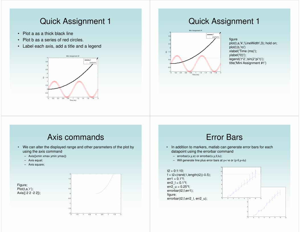
Quick Assignment 1
• Plot a as a thick black line
• Plot b as a series of red circles.
• Label each axis, add a title and a legend
4Mini Assignment #1
0 0.2 0.4 0.6 0.8 1 1.2 1.4 1.6 1.8 2-1
-0.5
0
0.5
1
1.5
2
2.5
3
3.5
4
Time (ms)
f(t)
t2
sin(2*pi*t)
Quick Assignment 1
1
1.5
2
2.5
3
3.5
4
f(t)
Mini Assignment #1
t2
sin(2*pi*t)
figure
plot(t,a,'k','LineWidth',3); hold on;
plot(t,b,'ro')
xlabel('Time (ms)');
ylabel('f(t)');
legend('t^2','sin(2*pi*t)');
0 0.2 0.4 0.6 0.8 1 1.2 1.4 1.6 1.8 2-1
-0.5
0
0.5
Time (ms)
legend('t^2','sin(2*pi*t)');
title('Mini Assignment #1')
Axis commands• We can alter the displayed range and other parameters of the plot by
using the axis command– Axis([xmin xmax ymin ymax])
– Axis equal;
– Axis square;
2
Figure;
Plot(t,a,’r’);
Axis([-2 2 -2 2]);
-2 -1.5 -1 -0.5 0 0.5 1 1.5 2-2
-1.5
-1
-0.5
0
0.5
1
1.5
2
Error Bars• In addition to markers, matlab can generate error bars for each
datapoint using the errorbar command– errorbar(x,y,e) or errorbar(x,y,ll,lu);
– Will generate line plus error bars at y+/-e or (y-ll,y+lu)
t2 = 0:1:10;
f = t2+(rand(1,length(t2))-0.5);
12
14
f = t2+(rand(1,length(t2))-0.5);
err1 = 0.1*f;
err2_l = 0.1*f;
err2_u = 0.25*f;
errorbar(t2,f,err1);
figure;
errorbar(t2,f,err2_l, err2_u);
-2 0 2 4 6 8 10 120
2
4
6
8
10
12
-2 0 2 4 6 8 10 120
2
4
6
8
10
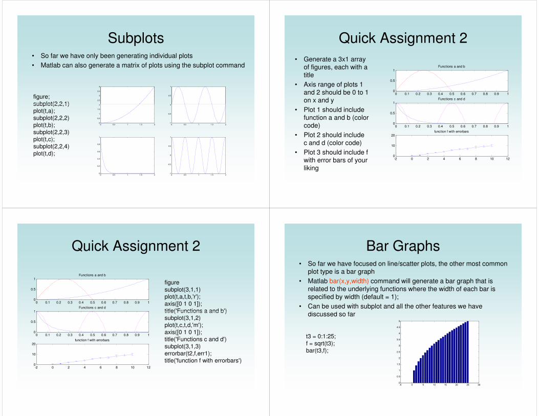
Subplots• So far we have only been generating individual plots
• Matlab can also generate a matrix of plots using the subplot command
figure;
subplot(2,2,1) 2
2.5
3
3.5
4
0
0.5
1
subplot(2,2,1)
plot(t,a);
subplot(2,2,2)
plot(t,b);
subplot(2,2,3)
plot(t,c);
subplot(2,2,4)
plot(t,d);
0 0.5 1 1.5 20
0.5
1
1.5
2
0 0.5 1 1.5 2-1
-0.5
0
0 0.5 1 1.5 20
0.2
0.4
0.6
0.8
1
0 0.5 1 1.5 2-1
-0.5
0
0.5
1
Quick Assignment 2
• Generate a 3x1 array of figures, each with a title
• Axis range of plots 1 and 2 should be 0 to 1 on x and y
0 0.1 0.2 0.3 0.4 0.5 0.6 0.7 0.8 0.9 10
0.5
1Functions a and b
1Functions c and d
• Plot 1 should include function a and b (color code)
• Plot 2 should include c and d (color code)
• Plot 3 should include f with error bars of your liking
0 0.1 0.2 0.3 0.4 0.5 0.6 0.7 0.8 0.9 10
0.5
1
-2 0 2 4 6 8 10 120
10
20function f with errorbars
Quick Assignment 2
0 0.1 0.2 0.3 0.4 0.5 0.6 0.7 0.8 0.9 10
0.5
1Functions a and b
1Functions c and d
figure
subplot(3,1,1)
plot(t,a,t,b,'r');
axis([0 1 0 1]);
title('Functions a and b')
0 0.1 0.2 0.3 0.4 0.5 0.6 0.7 0.8 0.9 10
0.5
1
-2 0 2 4 6 8 10 120
10
20function f with errorbars
title('Functions a and b')
subplot(3,1,2)
plot(t,c,t,d,'m');
axis([0 1 0 1]);
title('Functions c and d')
subplot(3,1,3)
errorbar(t2,f,err1);
title('function f with errorbars')
Bar Graphs• So far we have focused on line/scatter plots, the other most common
plot type is a bar graph
• Matlab bar(x,y,width) command will generate a bar graph that is related to the underlying functions where the width of each bar is specified by width (default = 1);
• Can be used with subplot and all the other features we have discussed so fardiscussed so far
t3 = 0:1:25;
f = sqrt(t3);
bar(t3,f);
-5 0 5 10 15 20 25 300
0.5
1
1.5
2
2.5
3
3.5
4
4.5
5

Histograms• Matlab hist(y,m) command will generate a frequency histogram of
vector y distributed among m bins
• Also can use hist(y,x) where x is a vector defining the bin centers
– Note you can use histc function if you want to define bin edges instead
• Can be used with subplot and all the other features we have discussed so far
hist(b,10);
Figure;
Hist(b,[-1 -0.75 0 0.25 0.5 0.75 1]);
-1.5 -1 -0.5 0 0.5 1 1.50
5
10
15
20
25
30
35
40
-1 -0.8 -0.6 -0.4 -0.2 0 0.2 0.4 0.6 0.8 10
5
10
15
20
25
30
35
40
45
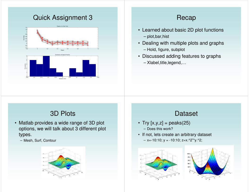
Quick Assignment 3
• Generate the following data set
– It results in multiple noisy repeats of some trial
• Create mean_x to be the mean of all the trials at each
point of x
• Create std_x to be the standard deviation of all trials at • Create std_x to be the standard deviation of all trials at
each point of x
• Add labels and titles
t = 0:0.1:1
for(i=1:25)
x(i,:) = exp(-10.*t) + 0.5*(rand(1,length(t))-0.5);
end
Quick Assignment 3
• Make a plot that is to include 2 subplots
• Plot #1:– Plot each individual trial (25 lines) in thin dotted black lines,
• tip: remember about how matlab interprets matricies for the plot command.
– Plot the mean of the trials with a thick, red, dashed line and error – Plot the mean of the trials with a thick, red, dashed line and error lines surrounding each datapoint that correspond to the standard deviation of each of the points
• Plot #2:– A histogram that expresses the distribution of the signal at the
end of each trial (last sample)
Quick Assignment 3
-0.2 0 0.2 0.4 0.6 0.8 1 1.2-0.4
-0.2
0
0.2
0.4
0.6
0.8
1
1.2
1.4Repeats of a Given Task
Repeat
Err
or
Rate
t = 0:0.1:1
for(i=1:25)
x(i,:) = exp(-10.*t) + 0.5*(rand(1,length(t))-0.5);
end
mean_x = mean(x);
std_x = std(x);
figure
subplot(2,1,1)
plot(t,x,'k'); hold on;Repeat
-0.25 -0.2 -0.15 -0.1 -0.05 0 0.05 0.1 0.15 0.2 0.250
1
2
3
4
5Distribution of Endpoint Position
Deviation (mm)
Occura
nces
plot(t,x,'k'); hold on;
errorbar(t,mean_x,std_x,'--r','LineWidth', 3);
title('Repeats of a Given Task')
xlabel('Repeat');
ylabel('Error Rate');
subplot(2,1,2)
hist(x(:,11),10)
title('Distribution of Endpoint Position');
xlabel('Deviation (mm)')
ylabel('Occurances')
Quick Assignment 3
-0.4
-0.2
0
0.2
0.4
0.6
0.8
1
1.2
1.4Repeats of a Given Task
Err
or
Rate
-0.2 0 0.2 0.4 0.6 0.8 1 1.2-0.4
Repeat
-0.25 -0.2 -0.15 -0.1 -0.05 0 0.05 0.1 0.15 0.2 0.250
1
2
3
4
5Distribution of Endpoint Position
Deviation (mm)
Occura
nces
Recap
• Learned about basic 2D plot functions
– plot,bar,hist
• Dealing with multiple plots and graphs
– Hold, figure, subplot– Hold, figure, subplot
• Discussed adding features to graphs
– Xlabel,title,legend,…
3D Plots
• Matlab provides a wide range of 3D plot options, we will talk about 3 different plot types.– Mesh, Surf, Contour
Dataset
• Try [x,y,z] = peaks(25)– Does this work?
• If not, lets create an arbitrary dataset
– x=-10:10; y = -10:10; z=x.^2’*y.^2;
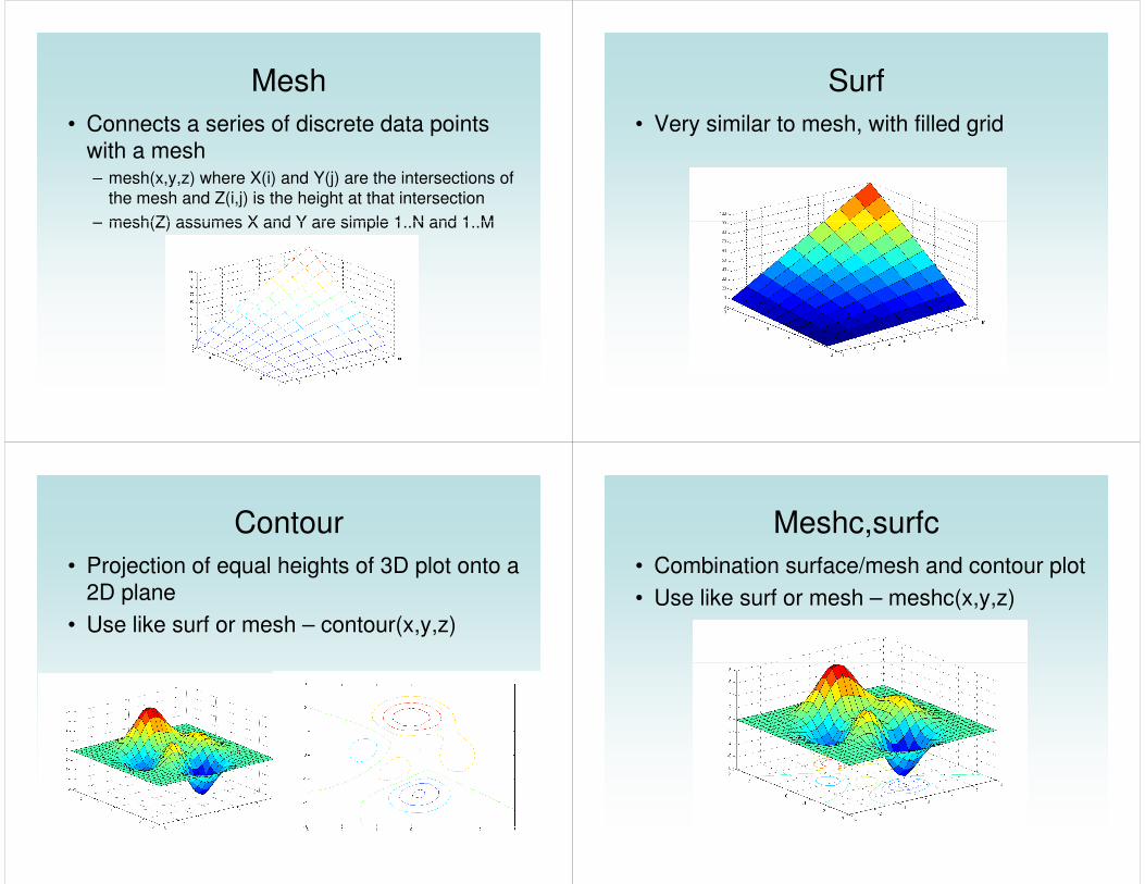
Mesh
• Connects a series of discrete data points with a mesh– mesh(x,y,z) where X(i) and Y(j) are the intersections of
the mesh and Z(i,j) is the height at that intersection
– mesh(Z) assumes X and Y are simple 1..N and 1..M– mesh(Z) assumes X and Y are simple 1..N and 1..M
Surf
• Very similar to mesh, with filled grid
Contour
• Projection of equal heights of 3D plot onto a 2D plane
• Use like surf or mesh – contour(x,y,z)
Meshc,surfc
• Combination surface/mesh and contour plot
• Use like surf or mesh – meshc(x,y,z)
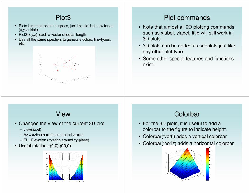
Plot3• Plots lines and points in space, just like plot but now for an
(x,y,z) triple
• Plot3(x,y,z), each a vector of equal length
• Use all the same specfiers to generate colors, line-types, etc.
Plot commands
• Note that almost all 2D plotting commands such as xlabel, ylabel, title will still work in 3D plots
• 3D plots can be added as subplots just like • 3D plots can be added as subplots just like any other plot type
• Some other special features and functions exist…
View
• Changes the view of the current 3D plot– view(az,el)
– Az = azimuth (rotation around z-axis)
– El = Elevation (rotation around xy-plane)
• Useful rotations (0,0),(90,0)• Useful rotations (0,0),(90,0)
Colorbar
• For the 3D plots, it is useful to add a colorbar to the figure to indicate height.
• Colorbar(‘vert’) adds a vertical colorbar
• Colorbar(‘horiz) adds a horizontal colorbar• Colorbar(‘horiz) adds a horizontal colorbar
caxis
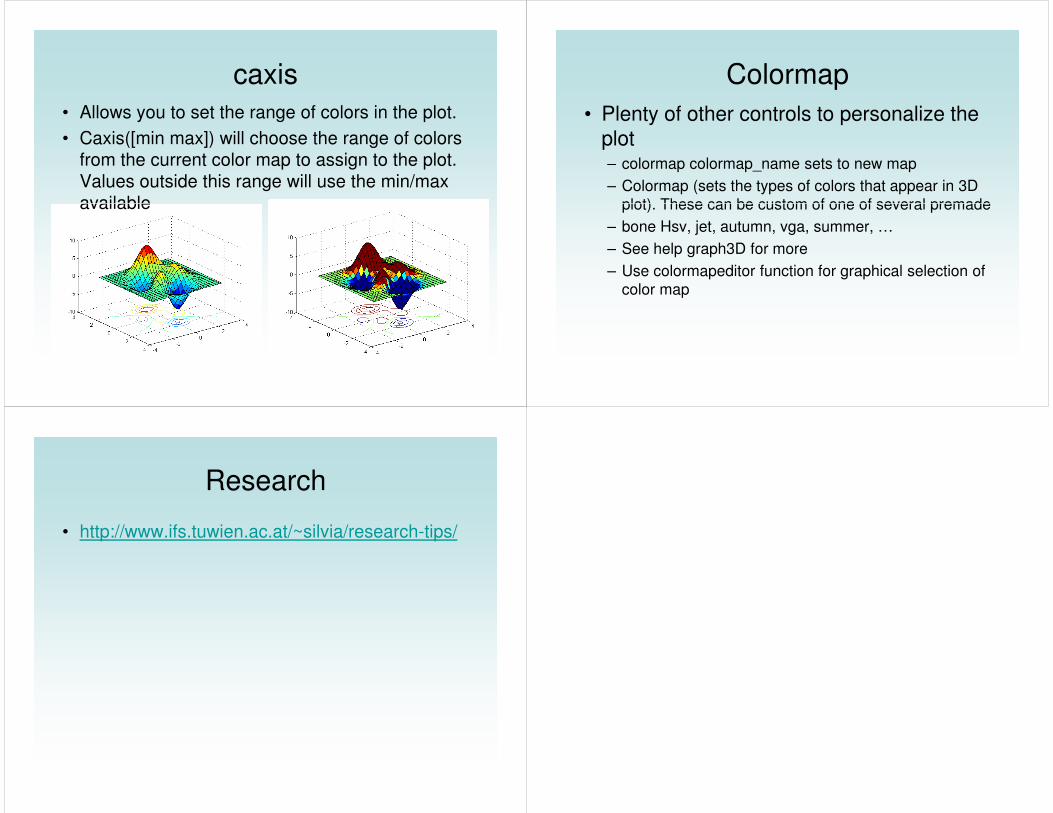
• Allows you to set the range of colors in the plot.
• Caxis([min max]) will choose the range of colors
from the current color map to assign to the plot.
Values outside this range will use the min/max
availableavailable
Colormap
• Plenty of other controls to personalize the plot– colormap colormap_name sets to new map
– Colormap (sets the types of colors that appear in 3D
plot). These can be custom of one of several premadeplot). These can be custom of one of several premade
– bone Hsv, jet, autumn, vga, summer, …
– See help graph3D for more
– Use colormapeditor function for graphical selection of
color map
Research
• http://www.ifs.tuwien.ac.at/~silvia/research-tips/