MATLAB

AutoCAD

Visio

Rational Rose

Computer Applications in Engineering Design

Introductory LectureIntroductory Lecture

LabVIEW

PSPICE

Orcad

Course InformationNuts and Bolts

Course Code: CP-203Prerequisites: Computer ProgrammingCredit Hours: 2 (Theory) + 1 (Lab)

Class Homepage: http://web.uettaxila.edu.pk/cms/

All handouts, announcements, assignments, etc. posted to website

“Lectures” link continuously updates topics, handouts, and reading

Class Mailing List:Google / Yahoo Group (Required Email addresses of all students)

Email: mona.waseem@uettaxila.edu.pk

Course SyllabusMATLABOrcadVisioPspiceAutoCADRational RoseLabVIEWUML

Tools

• Matlab and Orcad is used for electrical/computer systems design

• AutoCAD like design tools are taught for 3D engineering drawings.

• Introduction to computer-aided design tools including AutoCAD,

OrCAD, MATLAB, LabVIEW, Rational Rose and Visio, etc.

• Study of theoretical concepts of electronic components and circuits

using simulation softwares: PSPICE, MATLAB, and LabVIEW.

• Tools like Visio and Rational Rose are used for software drawing like

process diagrams, class diagram, sequence diagram, interaction

diagrams and deployment diagram, Entity-Relationship diagram etc.

• Design of software designs using Visio and Rational Rose for

understanding and implementing object oriented designs and

standards like UML.

Introduction to Matlab

Click on the Matlab icon/start menu initialises the Matlab environment:

The main window is the dynamic command interpreter which allows the user to issue Matlab commands

The variable browser shows which variables currently exist in the workspace

Variable browser

Commandwindow

Command history

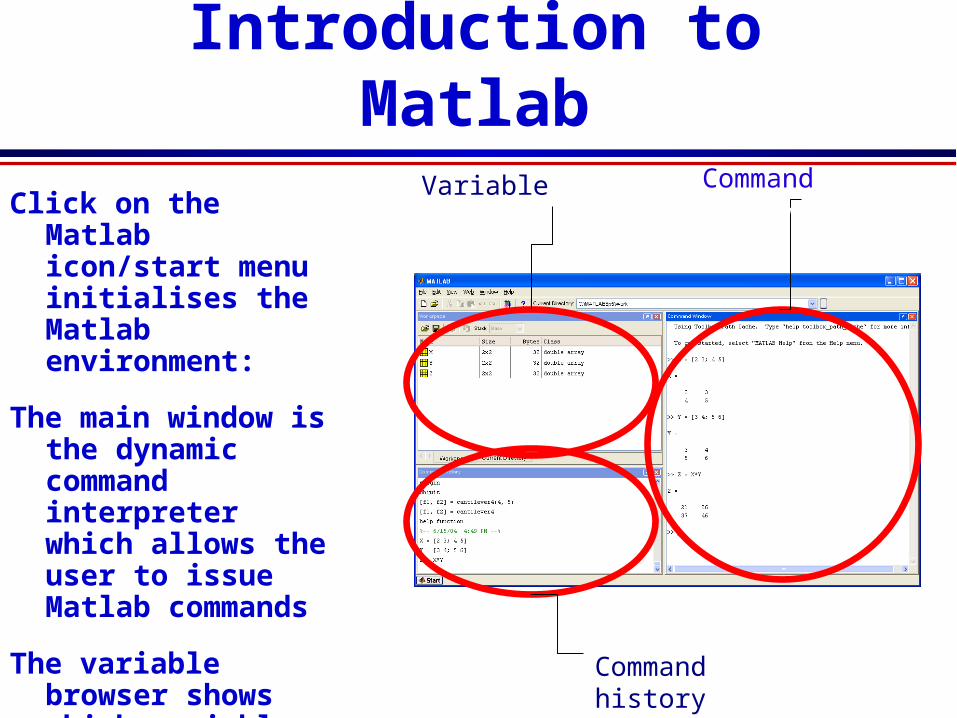
Matlab Programming Environment

Matlab (Matrix Laboratory) is a dynamic, interpreted, environment for matrix/vector analysis

Variables are created at run-time, matrices are dynamically re-sized, …

User can build programs (in .m files or at command line) using a C/Java-like syntax

Ideal environment for model building, system identification and control (both discrete and continuous time

Wide variety of libraries (toolboxes) available

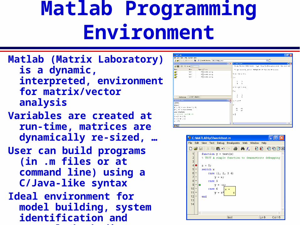
Basic Matlab

Examplea=[1,2,3,4,5];b=[a;a;a]

b=1 2 3 4 51 2 3 4 51 2 3 4 5

Examplea=[1;2;3;4;5];b=[a,a,a]

b= 1 1 1 2 2 2 3 3 3 4 4 4 5 5 5 Example (transpose)

a=[1;2;3;4;5];b=a’b= 1 2 3 4 5

Basic Matlab

Stringsa=[‘a’,’b’,’c’]a= abc

b=[a;a;a]

b= abc

abc

abc

Stringsa=[‘a’,’b’,’c’]a= abc

b=[a,a,a]

b= abcabcabc

Stringsa=[‘a’,’b’,’c’]b=[‘a’,’c’,’c’]

c=(a==b);

c= 1 0 1

Basic Matlab

1 2

3 4

5 6

7 8

6 8

10 12

19 22*

43 50

A

B

A B

A B

5 12.*

21 32

1 4.^ 2

9 16

sin(1) sin(2)sin( )

sin(3) sin(4)

A B

A

A

Basic Matlab

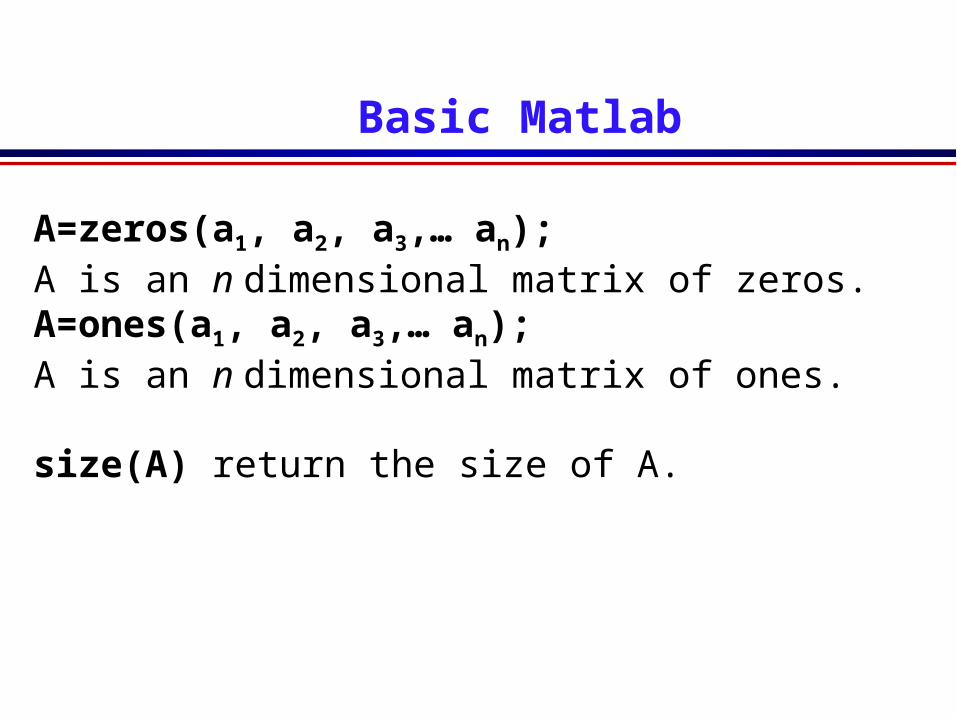
A=zeros(a1, a2, a3,… an);A is an n dimensional matrix of zeros.A=ones(a1, a2, a3,… an);A is an n dimensional matrix of ones.

size(A) return the size of A.

Basic Matlab

A(m,n) returns the value of the matrix in row-m and column-n.

b=A(1:end,1) : b will be equal to column 1 of A

b=A(5:10,5:10) : b will a-6x6 matrix containing all values of A from rows 5-10 and columns 5-10.

Basic MatlabFunctions in Matlab

function [output variables]=function_name (input variables)

Input and output variables, can be of any type.

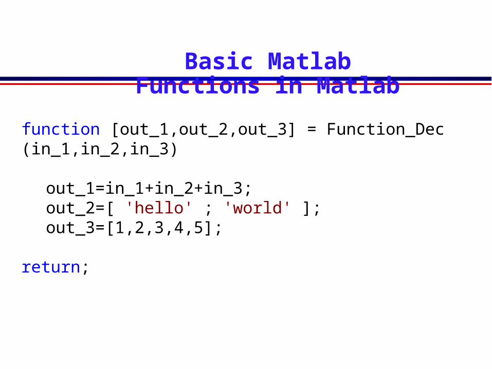
function [out_1,out_2,out_3] = Function_Dec (in_1,in_2,in_3)

out_1=in_1+in_2+in_3;out_2=[ 'hello' ; 'world' ];out_3=[1,2,3,4,5];

return;

Basic MatlabFunctions in Matlab

input:» [a,b,c]=Function_dec(5,3,2)

output:a = 10b = helloworld

c = 1 2 3 4 5

input:» [a,b,c]=Function_dec([1,2,3],[6,5,4],[3,4,5])

output:a = 10 11 12b = hello world

c = 1 2 3 4 5

Basic MatlabFunctions in Matlab

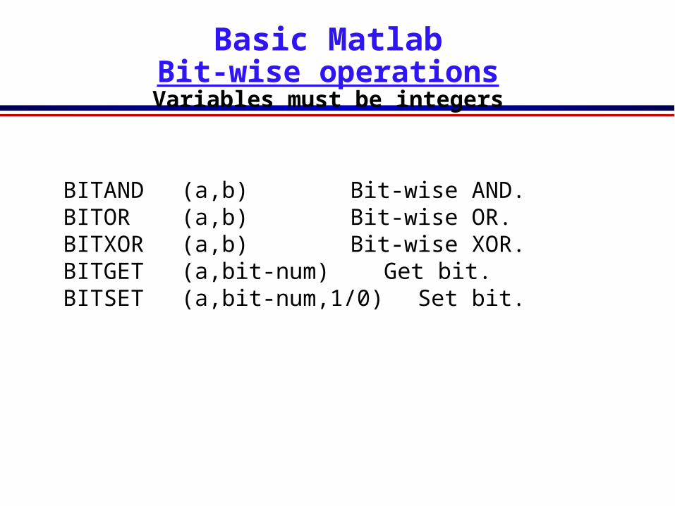
Basic MatlabBit-wise operationsVariables must be integers

BITAND (a,b) Bit-wise AND.BITOR (a,b) Bit-wise OR.BITXOR (a,b) Bit-wise XOR.BITGET (a,bit-num) Get bit.BITSET (a,bit-num,1/0) Set bit.

Basic Matlabconditions

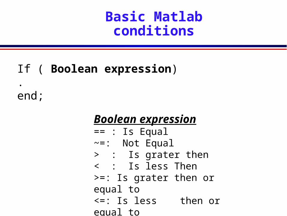
If ( Boolean expression).end;

Boolean expression== : Is Equal ~=: Not Equal> : Is grater then< : Is less Then>=: Is grater then or equal to<=: Is less then or equal to

Basic Matlabconditions

switch switch_expr

case case_expr, statement, ..., statement case {case_expr1, case_expr2, case_expr3,...} statement, ..., statement ... otherwise, statement, ..., statementend

Basic MatlabLoops

for j=start:step:end.end; example:for j=-1:0.2:3.end;

while Boolean expression, .end; example:while a>b,.end;

break - Terminate execution of WHILE or FOR loop. break terminates the execution of FOR and WHILE loops. In nested loops, BREAK exits from the innermost loop only.

Topics Covered:

1. Plotting basic 2-D plots.

• The plot command.

• The fplot command.

• Plotting multiple graphs in the same plot.

• Formatting plots.

Two Dimensional Plots

MAKING X-Y PLOTS

MATLAB has many functions and commands that can be used to

create various types of plots.

In our class we will only create two dimensional x – y plots.

8 10 12 14 16 18 20 22 240

200

400

600

800

1000

1200

DISTANCE (cm)

INT

EN

SIT

Y (

lux)

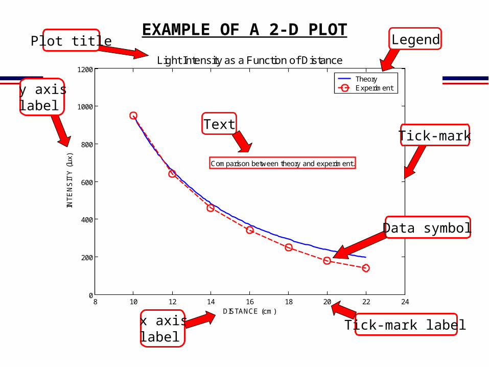
Light Intensity as a Function of Distance

Comparison between theory and experiment.

TheoryExperiment

Plot title

y axislabel

x axislabel

Text

Tick-mark label

EXAMPLE OF A 2-D PLOT

Data symbol

Legend

Tick-mark

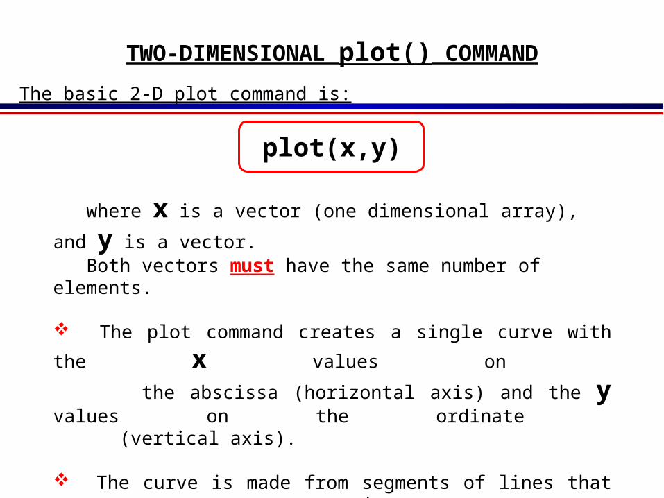
TWO-DIMENSIONAL plot() COMMAND

where x is a vector (one dimensional array), and y is a vector. Both vectors must have the same number of elements.

The plot command creates a single curve with the x values on

the abscissa (horizontal axis) and the y values on the ordinate (vertical axis).

The curve is made from segments of lines that connect the

points that are defined by the x and y coordinates of the elements in the two vectors.

The basic 2-D plot command is:

plot(x,y)

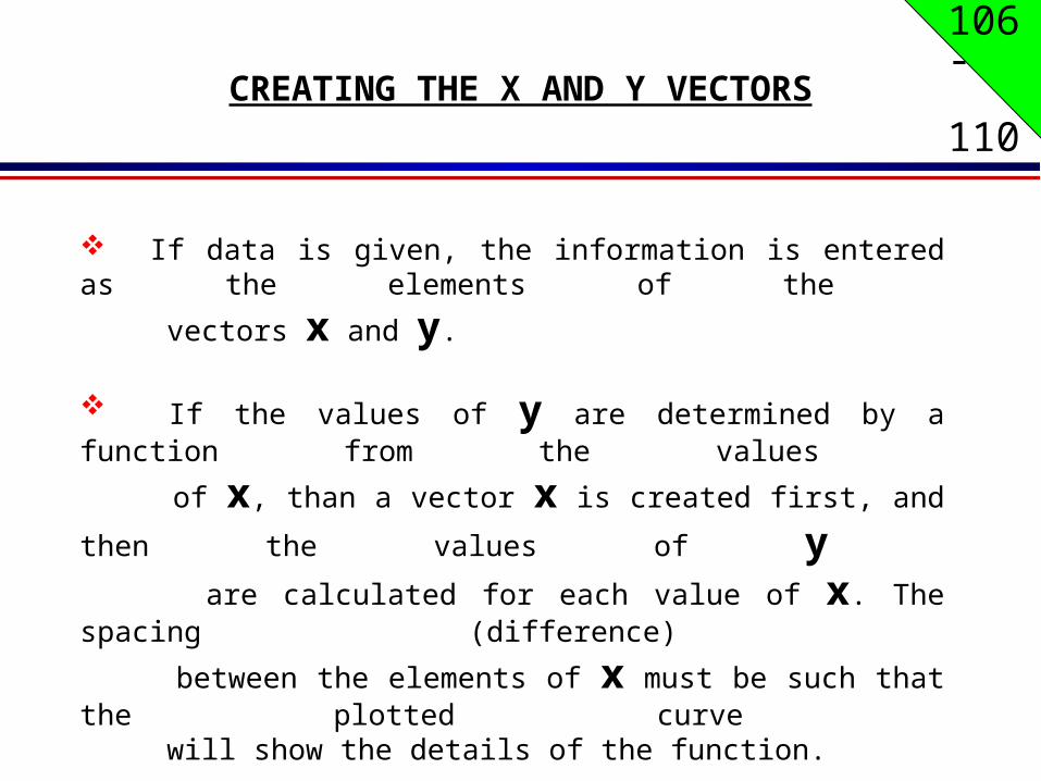
If data is given, the information is entered as the elements of the

vectors x and y.

If the values of y are determined by a function from the values

of x, than a vector x is created first, and then the values of y

are calculated for each value of x. The spacing (difference)

between the elements of x must be such that the plotted curve will show the details of the function.

CREATING THE X AND Y VECTORS

106- 110

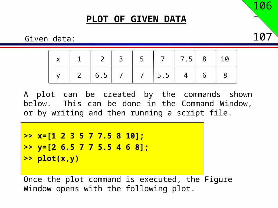
PLOT OF GIVEN DATA

Given data:

>> x=[1 2 3 5 7 7.5 8 10];

>> y=[2 6.5 7 7 5.5 4 6 8];

>> plot(x,y)

A plot can be created by the commands shown below. This can be done in the Command Window, or by writing and then running a script file.

Once the plot command is executed, the Figure Window opens with the following plot.

106- 107

x

y

1 2 3 5 7 7.5 8

6.5 7 7 5.5 4 6 8

10

2

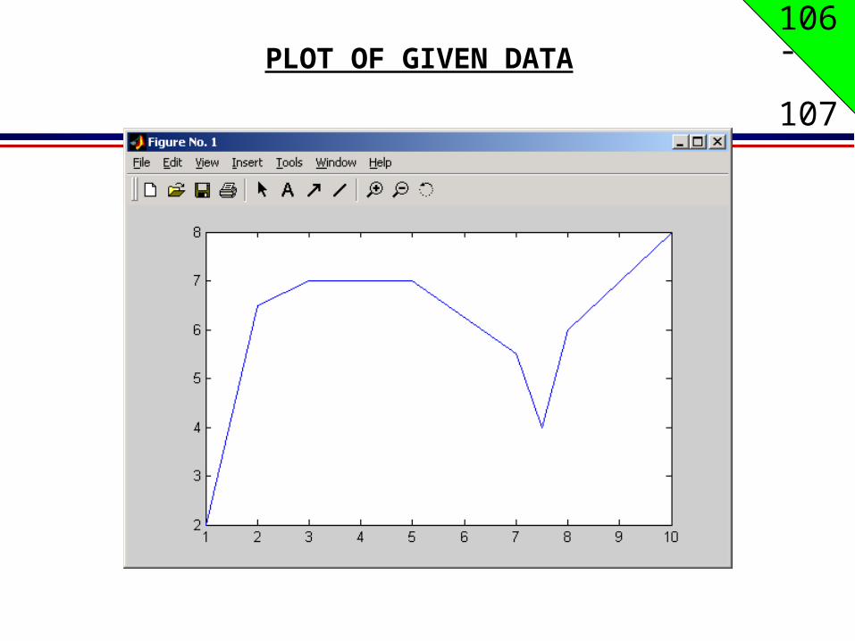
106- 107PLOT OF GIVEN DATA

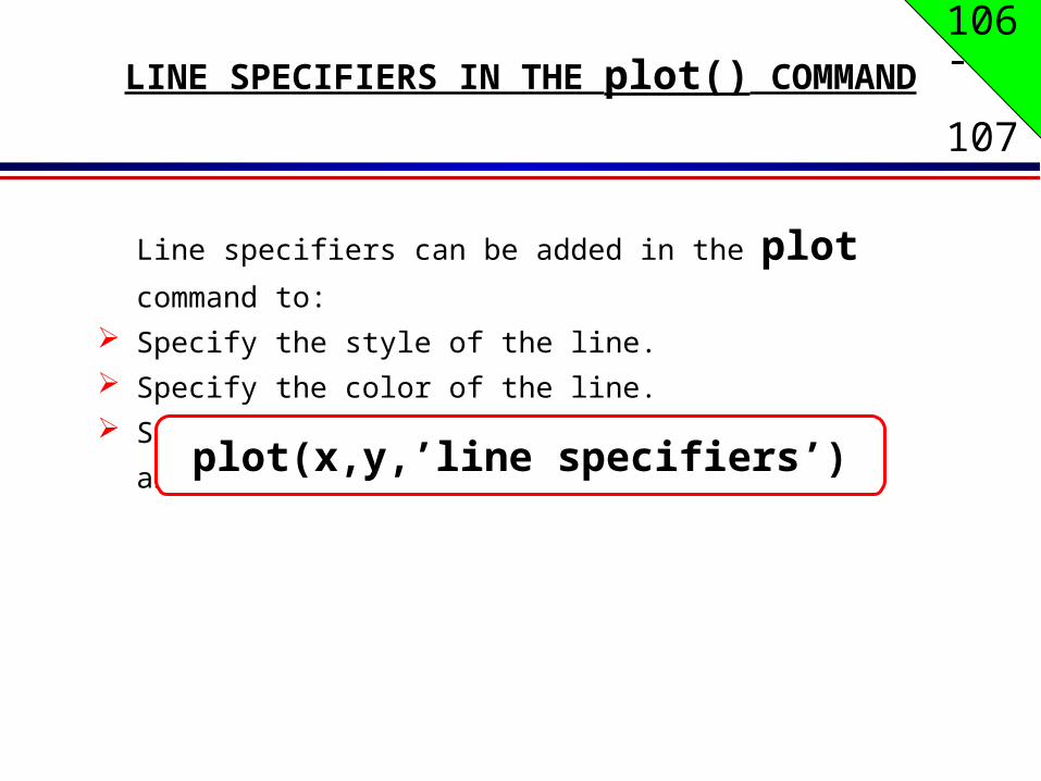
106- 107LINE SPECIFIERS IN THE plot() COMMAND

Line specifiers can be added in the plot command to:

Specify the style of the line.

Specify the color of the line.

Specify the type of the markers (if markers are desired).

plot(x,y,’line specifiers’)

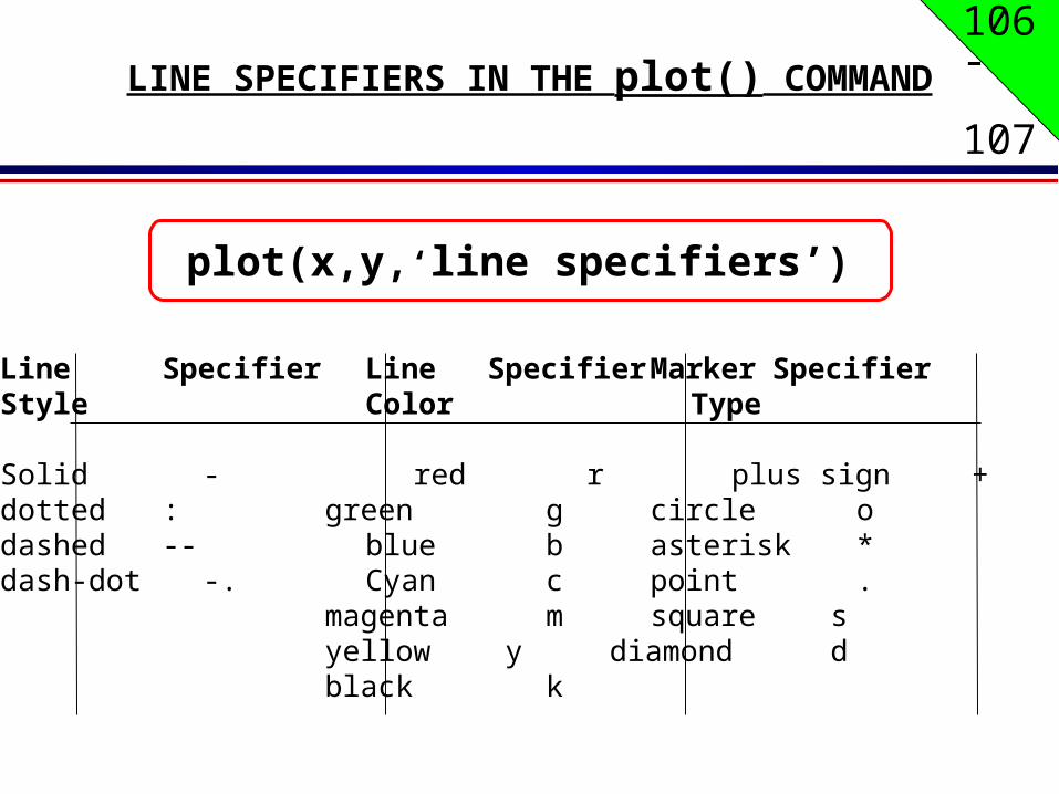
106- 107LINE SPECIFIERS IN THE plot() COMMAND

Line Specifier Line Specifier Marker SpecifierStyle Color Type

Solid - red r plus sign +dotted : green g circle odashed -- blue b asterisk *dash-dot -. Cyan c point .

magenta m square syellow y diamond dblack k

plot(x,y,‘line specifiers’)

107- 108LINE SPECIFIERS IN THE plot() COMMAND

The specifiers are typed inside the plot() command as strings.

Within the string the specifiers can be typed in any order.

The specifiers are optional. This means that none, one, two, or all the three can be included in a command.

EXAMPLES:plot(x,y) A solid blue line connects the points with no markers.

plot(x,y,’r’) A solid red line connects the points with no markers.

plot(x,y,’--y’) A yellow dashed line connects the points.

plot(x,y,’*’) The points are marked with * (no line between the points.)

plot(x,y,’g:d’)A green dotted line connects the points which are marked with diamond markers.

110- 111

Year

Sales (M)

1988 1989 1990 1991 1992 1993 1994

127 130 136 145 158 178 211

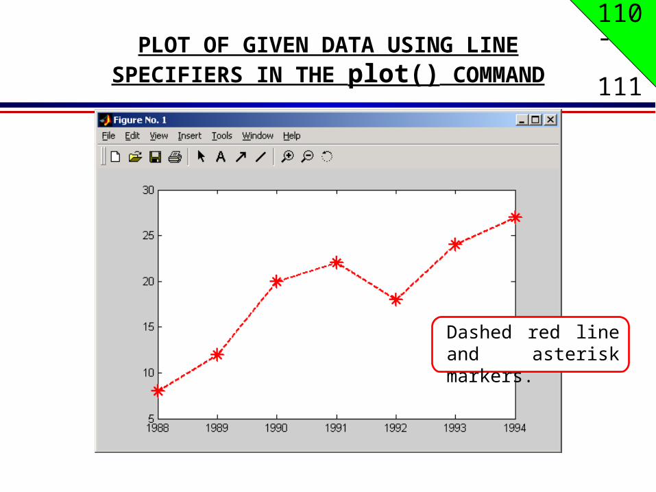
PLOT OF GIVEN DATA USING LINE SPECIFIERS IN THE plot() COMMAND

>> year = [1988:1:1994];

>> sales = [127, 130, 136, 145, 158, 178, 211];

>> plot(year,sales,'--r*')

Line Specifiers:dashed red line and asterisk markers.

110- 111PLOT OF GIVEN DATA USING LINE

SPECIFIERS IN THE plot() COMMAND

Dashed red line and asterisk markers.

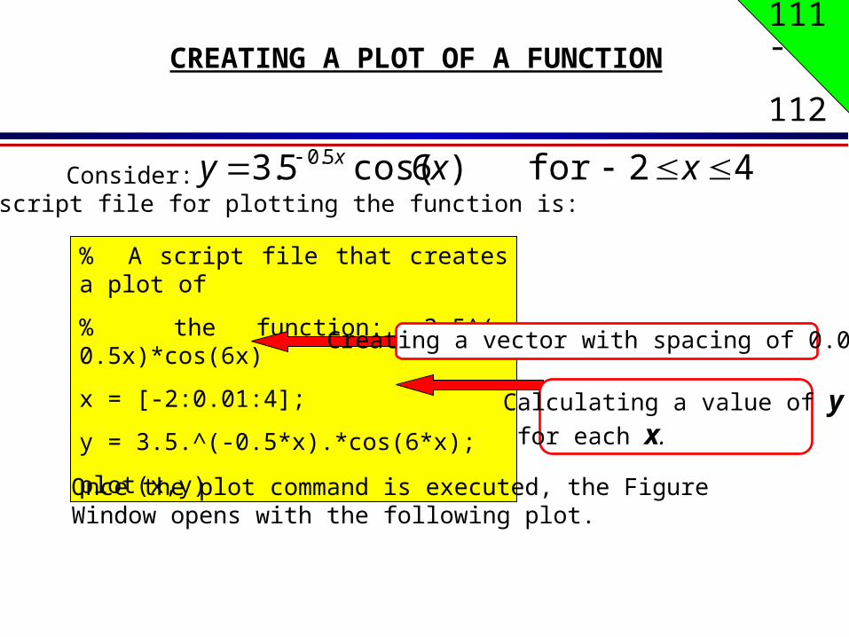
% A script file that creates a plot of

% the function: 3.5^(-0.5x)*cos(6x)

x = [-2:0.01:4];

y = 3.5.^(-0.5*x).*cos(6*x);

plot(x,y)

CREATING A PLOT OF A FUNCTION

Consider: 42for)6cos(5.3 5.0 xxy x

A script file for plotting the function is:

Creating a vector with spacing of 0.01.

Calculating a value of y for each x.

Once the plot command is executed, the Figure Window opens with the following plot.

111- 112

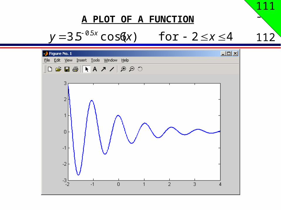
A PLOT OF A FUNCTION

42for)6cos(5.3 5.0 xxy x

111- 112

CREATING A PLOT OF A FUNCTION

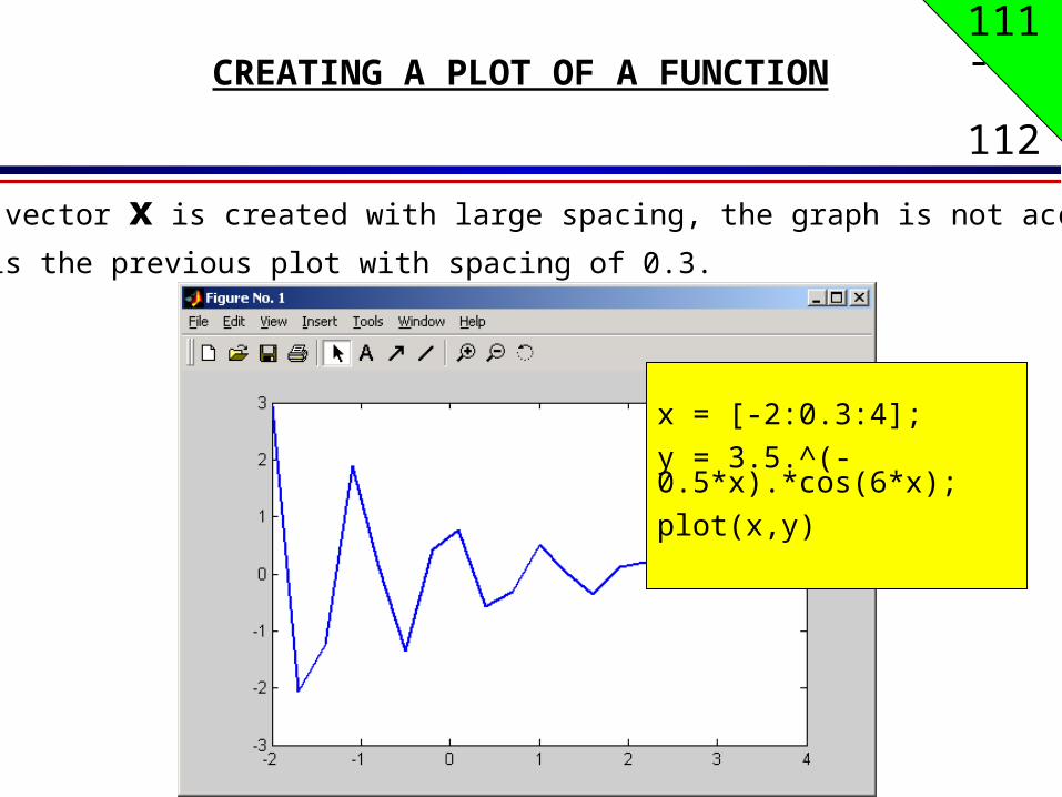
If the vector x is created with large spacing, the graph is not accurate.

Below is the previous plot with spacing of 0.3.

111- 112

x = [-2:0.3:4];

y = 3.5.^(-0.5*x).*cos(6*x);

plot(x,y)

112- 113THE fplot COMMAND

fplot(‘function’,limits)

The fplot command can be used to plot a function

with the form: y = f(x)

The function is typed in as a string.

The limits is a vector with the domain of x, and optionally with limits

of the y axis:

[xmin,xmax] or [xmin,xmax,ymin,ymax]

Line specifiers can be added.

112- 113

PLOT OF A FUNCTION WITH THE fplot() COMMAND

>> fplot('x^2 + 4 * sin(2*x) - 1', [-3 3])

33for1)2sin(42 xxxyA plot of:

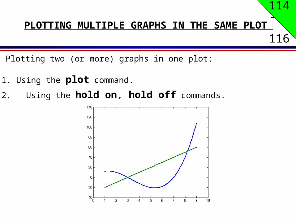
PLOTTING MULTIPLE GRAPHS IN THE SAME PLOT

Plotting two (or more) graphs in one plot:

1. Using the plot command.

2. Using the hold on, hold off commands.

114- 116

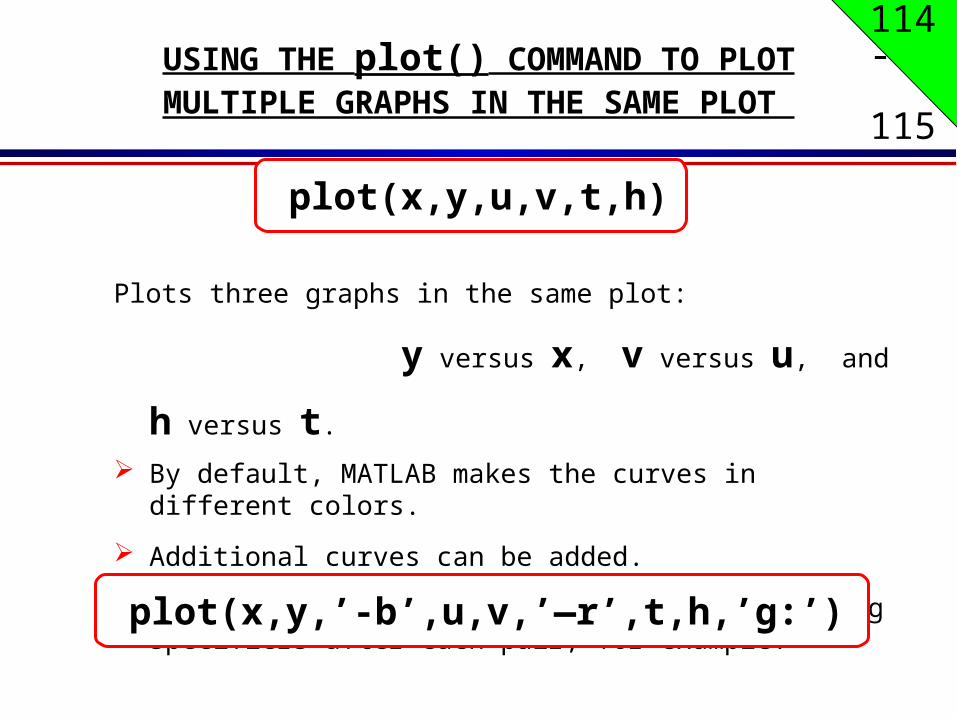
USING THE plot() COMMAND TO PLOTMULTIPLE GRAPHS IN THE SAME PLOT

Plots three graphs in the same plot:

y versus x, v versus u, and h versus t.

By default, MATLAB makes the curves in different colors.

Additional curves can be added.

The curves can have a specific style by adding specifiers after each pair, for example:

114- 115

plot(x,y,u,v,t,h)

plot(x,y,’-b’,u,v,’—r’,t,h,’g:’)

114- 115USING THE plot() COMMAND TO PLOT

MULTIPLE GRAPHS IN THE SAME PLOT

42 x

Plot of the function, and its first and second

derivatives, for , all in the same plot.

10263 3 xxy

42 x

x = [-2:0.01:4];

y = 3*x.^3-26*x+6;

yd = 9*x.^2-26;

ydd = 18*x;

plot(x,y,'-b',x,yd,'--r',x,ydd,':k')

vector x with the domain of the function.

Vector y with the function value at each x.

42 x

Vector yd with values of the first derivative.Vector ydd with values of the second

derivative.

Create three graphs, y vs. x (solid blue

line), yd vs. x (dashed red line), and ydd

vs. x (dotted black line) in the same figure.

114- 115

-2 -1 0 1 2 3 4-40

-20

0

20

40

60

80

100

120

USING THE plot() COMMAND TO PLOTMULTIPLE GRAPHS IN THE SAME PLOT

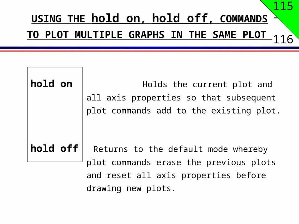
hold on Holds the current plot and all axis properties so that

subsequent plot commands add to the existing plot.

hold off Returns to the default mode whereby plot commands

erase the previous plots and reset all axis properties

before drawing new plots.

USING THE hold on, hold off, COMMANDS

TO PLOT MULTIPLE GRAPHS IN THE SAME PLOT

115- 116

115- 116

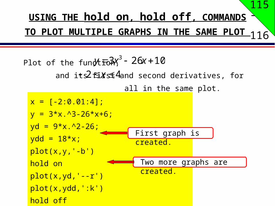
Plot of the function, and its first and second

derivatives, for all in the same plot.

10263 3 xxy

42 x

x = [-2:0.01:4];

y = 3*x.^3-26*x+6;

yd = 9*x.^2-26;

ydd = 18*x;

plot(x,y,'-b')

hold on

plot(x,yd,'--r')

plot(x,ydd,':k')

hold off

Two more graphs are created.

First graph is created.

USING THE hold on, hold off, COMMANDS

TO PLOT MULTIPLE GRAPHS IN THE SAME PLOT

8 10 12 14 16 18 20 22 240

200

400

600

800

1000

1200

DISTANCE (cm)

INT

EN

SIT

Y (

lux)

Light Intensity as a Function of Distance

Comparison between theory and experiment.

TheoryExperiment

Plot title

y axislabel

x axislabel

Text

EXAMPLE OF A FORMATTED 2-D PLOT

Data symbol

106

Legend

Tick-mark

Tick-mark label

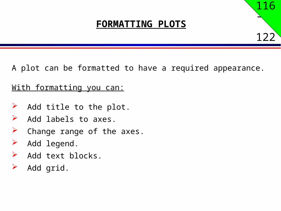
FORMATTING PLOTS

A plot can be formatted to have a required appearance.

With formatting you can:

Add title to the plot.

Add labels to axes.

Change range of the axes.

Add legend.

Add text blocks.

Add grid.

116- 122

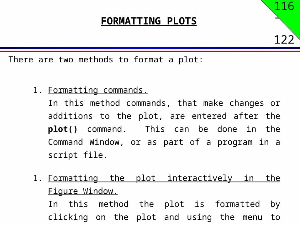
FORMATTING PLOTS

There are two methods to format a plot:

1. Formatting commands.

In this method commands, that make changes or additions to

the plot, are entered after the plot() command. This can be

done in the Command Window, or as part of a program in a

script file.

1. Formatting the plot interactively in the Figure Window.

In this method the plot is formatted by clicking on the plot and

using the menu to make changes or add details.

116- 122

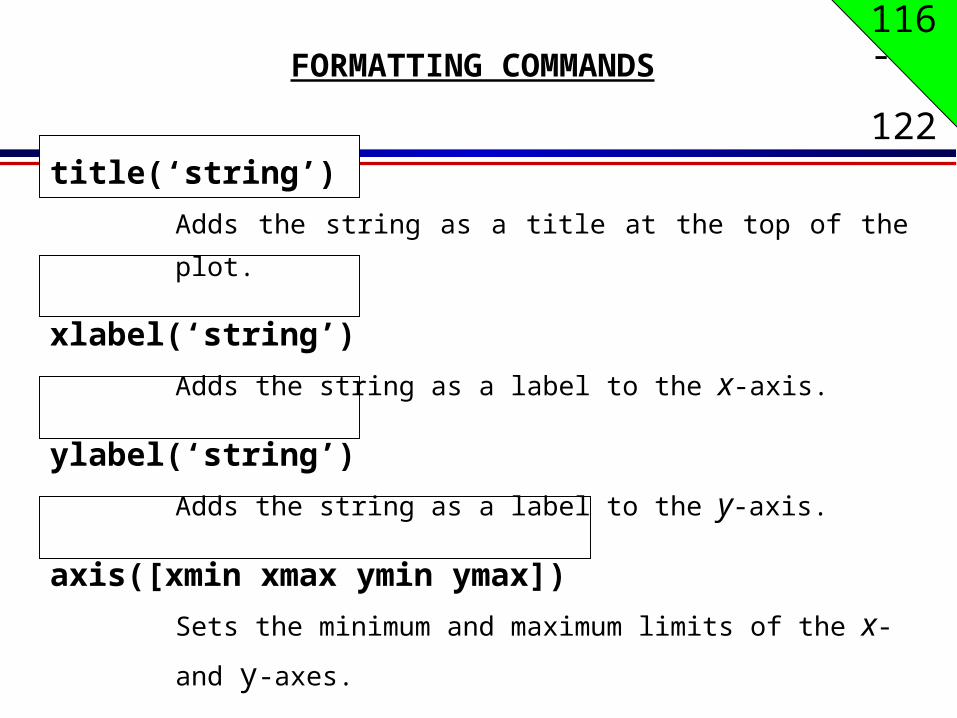
FORMATTING COMMANDS

116- 122

title(‘string’)

Adds the string as a title at the top of the plot.

xlabel(‘string’)

Adds the string as a label to the x-axis.

ylabel(‘string’)

Adds the string as a label to the y-axis.

axis([xmin xmax ymin ymax])

Sets the minimum and maximum limits of the x- and y-axes.

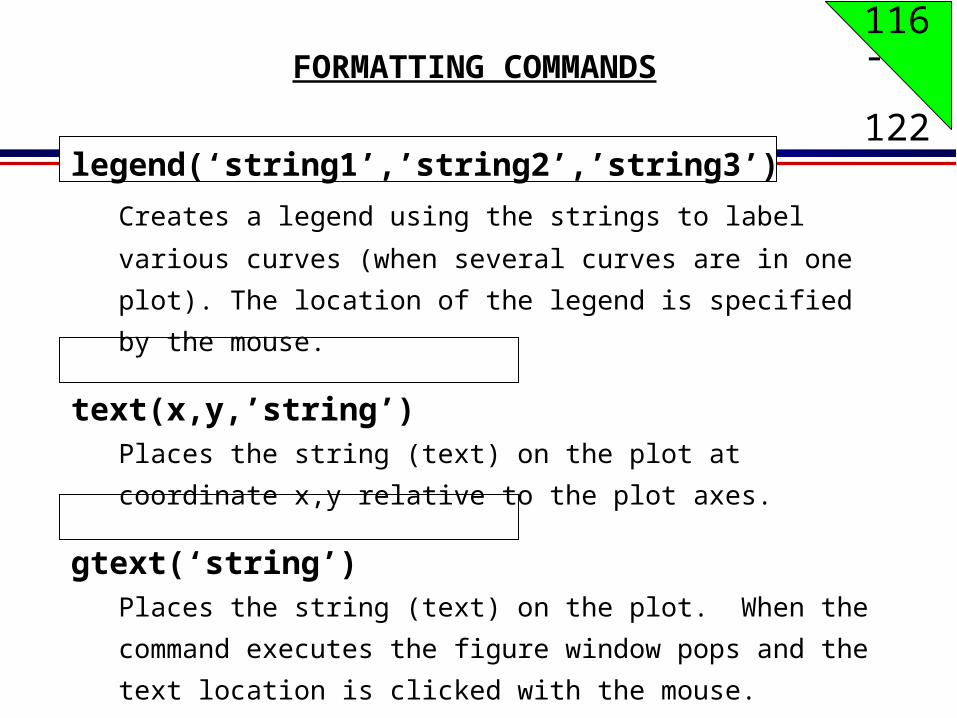
FORMATTING COMMANDS

116- 122

legend(‘string1’,’string2’,’string3’)

Creates a legend using the strings to label various curves

(when several curves are in one plot). The location of the

legend is specified by the mouse.

text(x,y,’string’)

Places the string (text) on the plot at coordinate x,y relative to

the plot axes.

gtext(‘string’)

Places the string (text) on the plot. When the command

executes the figure window pops and the text location is clicked

with the mouse.

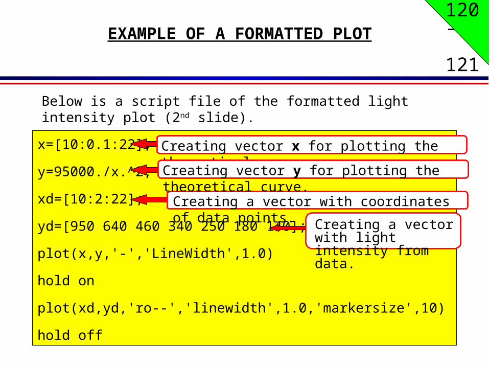
EXAMPLE OF A FORMATTED PLOT

Below is a script file of the formatted light intensity plot (2nd slide).

120- 121

x=[10:0.1:22];

y=95000./x.^2;

xd=[10:2:22];

yd=[950 640 460 340 250 180 140];

plot(x,y,'-','LineWidth',1.0)

hold on

plot(xd,yd,'ro--','linewidth',1.0,'markersize',10)

hold off

Creating a vector with light intensity from data.

Creating a vector with coordinates of data points.

Creating vector x for plotting the theoretical curve.

Creating vector y for plotting the theoretical curve.

120- 121EXAMPLE OF A FORMATTED PLOT

Formatting of the light intensity plot (cont.)

Creating a legend.

xlabel('DISTANCE (cm)')

ylabel('INTENSITY (lux)')

title('\fontname{Arial}Light Intensity as a Function of Distance','FontSize',14)

axis([8 24 0 1200])

text(14,700,'Comparison between theory and experiment.','EdgeColor','r','LineWidth',2)

legend('Theory','Experiment',0)

Creating text.

Title for the plot.

Setting limits of the axes.

Labels for the axes.

The plot that is obtained is shown again in the next slide.

120- 121EXAMPLE OF A FORMATTED PLOT

FORMATTING A PLOT IN THE FIGURE WINDOW

Once a figure window is open, the figure can be formatted interactively.

Use Figure, Axes, and Current Object-Properties in the Edit menu

Click here to start the plot edit mode.

Use the insert menu to

121- 122

QUIZ

Q1.a=[‘ab’,’ac’,’ad’], b=[a,a,a]B=?

Q2. Differentiate hold on and hold off.