General rights Copyright and moral rights for the publications made accessible in the public portal are retained by the authors and/or other copyright owners and it is a condition of accessing publications that users recognise and abide by the legal requirements associated with these rights.

Users may download and print one copy of any publication from the public portal for the purpose of private study or research.

You may not further distribute the material or use it for any profit-making activity or commercial gain

You may freely distribute the URL identifying the publication in the public portal If you believe that this document breaches copyright please contact us providing details, and we will remove access to the work immediately and investigate your claim.

Downloaded from orbit.dtu.dk on: Jun 19, 2020

Mathematical Programming Approaches for Optimal University Timetabling

Bagger, Niels-Christian Fink

Publication date:2017

Document VersionPublisher's PDF, also known as Version of record

Link back to DTU Orbit

Citation (APA):Bagger, N-C. F. (2017). Mathematical Programming Approaches for Optimal University Timetabling. DTUManagement Engineering.

Mathematical Programming Approaches for

Optimal University Timetabling

PhD Thesis

Niels-Christian F. BaggerJanuary, 2017

Title: Mathematical Programming Approaches for Optimal University TimetablingType: PhD ThesisDate: January, 2017

Author: Niels-Christian F. Bagger

Supervisors: Associate Professor Thomas R. StidsenManagement ScienceDTU Management EngineeringTechnical University of DenmarkProduktionstorvet, Building 426BDK-2800 Kgs. Lyngby

Matias SørensenMaCom A/SVesterbrogade 48, 1.DK-1620 København V

University: Technical University of DenmarkDepartment: DTU Management EngineeringDivision: Management ScienceAddress: Produktionstorvet, Building 426B

DK-2800 Kgs. LyngbyTelephone: +45 45254800

Abstract

Every semester universities are faced with the challenge of creating timetables for the courses.Creating these timetables is an important task to ensure that students can attend the coursesthey need for their education. Creating timetables that are feasible can be challenging, andwhen different preferences are taken into account, the problems become even more challenging.Therefore, automating the processes of generating these timetables is a great help for the plan-ners and the universities. Scheduling and timetabling has been studied before in the literature,and two international conferences are dedicated to this research field.

This thesis considers a University Timetabling problem, more specifically the Curriculum-based Course Timetabling (CTT) problem. The objective of the CTT problem is to assign a setof lectures to time slots and rooms. The literature has focused mainly on heuristic applicationswhich are also apparent in the different surveys. The drawback of the heuristics is that theyare problem specific and do not provide any information on the quality of the solutions theygenerate. The objective of this thesis is to minimize the gap between the best-known upperbounds and the best-known lower bounds for CTT by using Mixed Integer Programming (MIP)based approaches.

We present a total of 15 different MIP based approaches that we have implemented, rangingfrom Cutting Plane techniques and Lagrangian Relaxation to Benders’ Decomposition andDantzig-Wolfe Decomposition. Most of these implementations did not provide satisfying results.However, they provide valuable insights into the difficulties of the problem. We discuss all theapproaches, the difficulties we have encountered, and suggestions on how to bring researchfurther.

Four of the implementations have led to articles submitted to international peer-reviewedjournals. The first two articles focus on exact methods and extend each other. The last twofocus on generating high-quality lower bounds by applying an extended formulation, which isthen decomposed. The articles in this thesis have brought us closer to the goal of closing thegap between the best-known upper and lower bounds for CTT. Though CTT was the problemin focus, the methods implemented here are general enough to be applied for other schedulingproblems as well.

iii

Resumé (Danish Abstract)

Hvert semester står universiteter over for udfordringen med at planlægge deres kurser. Denneplanlægning er en vigtig opgave for at sikre, at de studerende kan deltage i de kurser derer nødvendige for at komme igennem deres uddannelse. Opgaven med at få skemaerne tilat gå op kan være udfordrende i sig selv, og når forskellige præferencer tages i betragtning,bliver opgaven blot endnu vanskeligere. Derfor er automatiserede planlægningssystemer en storhjælp for planlæggerne og universiteterne. Planlægning og skemalægning er blevet studeret ilitteraturen før, og to internationale konferencer er dedikeret til dette område.

Denne afhandling studerer et universitetsskemalægningsproblem, mere specifikt Pensum-baseret Kursus Skemalægningsproblemet (PKS). Formålet med PKS er at tildele et sæt afforelæsninger til ugentlige tidsintervaller og lokaler. I litteraturen er der fokuseret primærtpå heuristiske metoder. Ulempen ved disse heuristikker er, at de er problem-specifikke og degiver ikke nogen oplysninger om kvaliteten af de løsninger de genererer. Formålet med denneafhandling er at minimere den afstand der er mellem de bedst kendte øvre grænser og de bedstkendte nedre grænser for PKS ved hjælp metoder baseret på matematisk programmering (MP).

Vi præsenterer i alt 15 forskellige metoder baseret på MP, som vi har implementeret. Defleste af disse implementeringer gav ikke tilfredsstillende resultater, men de giver værdifuldindsigt til vanskelighederne ved PKS og ideér til videre forskning. Vi diskuterer alle de metoder,de vanskeligheder vi er stødt på, og forslag til, hvorledes forskningen kan videreføres.

Fire af implementeringerne har ført til artikler indsendt til internationale tidsskrifter. Deto første artikler fokuserer på eksakte metoder og ligger i forlængelse af hinanden. De sidsteto fokuserer på at generere nedre grænser af høj kvalitet og ligger ogsÃě i forlÃęngelse afhinanden. Artiklerne i denne afhandling har bragt os tættere på målet om at mindske afstandenmellem de bedst kendte øvre og nedre grænser for PKS. Selvom PKS har været problemet ifokus her, så er de metoder der er implementeret generelle nok til at blive anvendt til andreplanlægningsproblemer.

v

Preface

This thesis is part of the requirements for acquiring the degree Philosophiae Doctor (Ph.D.) atthe Technical University of Denmark. This work has been a collaboration between the TechnicalUniversity of Denmark and MaCom A/S, a Danish provider of administration software for theeducational sector. The project has been financially supported by MaCom A/S and InnovationFund Denmark (IFD) under the Industrial Ph.D. Program. The work has been conducted atthe Division Management Science in the Department DTU Management Engineering of theTechnical University of Denmark from February 2014 to January 2017. The thesis consists ofan introduction and four papers submitted to peer-reviewed journals. As part of the study,a visit to the Groupe d’Études et de Recherche en Analyse des Décisions for four and a halfmonth was conducted in the first half of 2015.

The project has been supervised by Associate Professor Thomas R. Stidsen with MatiasSørensen as a co-supervisor.

Kgs. Lyngby, Denmark, January 2017

Niels-Christian F. Bagger

vii

Acknowledgments

First of all, I would like to thank my supervisors, Thomas R. Stidsen and Matias Sørensenfor their guidance throughout these last three years. Especially, I would like to thank Thomasfor the support, not only on an academic level, but also on a more personal level, and on hisendeavor to ensure that I can continue in the academic life after this project.

I would also like to thank Mads Poulsen and Martin Holbøll from MaCom A/S for givingme the opportunity of working on this project. Furthermore, I would like to thank all mycolleagues at MaCom for just being fun and friendly. It has been three great years, and I amgoing to miss the people there.

Big thanks to my colleagues at the Technical University of Denmark (DTU). I look forwardto staying there for, hopefully, many years to come. I would like to thank Assistant ProfessorEvelien van der Hurk and Christina Scheel Persson for their valuable feedback on some of thepapers. Thanks to Stefan Røpke for always keeping the door open for me whenever I had anyquestions. I would also like to thank David Pisinger for guidance, both regarding my careerchoice and on a more personal level. Lastly, I would like to thank all my colleagues at DTUfor welcoming my dog, Freya. She is perhaps the most eager of all to get to work, most likelybecause she is treated so well by all.

I would also like to thank Professor Guy Desaulniers and Professor Jacques Desrosiers,whom I visited in Montréal for four and a half month during this project. I really appreciatethe time and effort they put into me and my project, both during my stay and the time after.Their involvement really exceeded my expectations. I would also like to thank Carole Dufourand Marie Perreault for being really friendly and great to talk to during my stay. I would liketo thank the entire GERAD group for their friendliness and also those from the CIRRELTgroup that I had a chance to meet.

A great thanks go to my family and friends. First, I would like to thank my good friend andcolleague Michael Lindahl for joining me on this journey. Michael started his Ph.D. projectat the same time as me, and he has been a great support throughout the entire process. Iwould not have been able to accommodate some of the challenges without him. Thanks tomy best friend Stephan Gerdes Høegh for his friendship and emotional support, not just thelast three years, but throughout my entire life. Also big thanks to my other best friend KariFalk Aaen, who has also always been there for me since the day I was born. Great thanks tomy mother-in-law for all the help that she has provided, especially during the last part of thewriting phase. Last, but definitely not least, I would like to thank my wife and daughter forputting up with me during the last three years, and for joining me during my research stay inMontréal. I have not been easy to live with, especially these last three to six months, and I

ix

would probably have given up along the way without you.

x

Contents

Abstract iii

Resumé (Danish Abstract) v

Preface vii

Acknowledgments ix

I Introduction 1

1 Background 31.1 Curriculum-based Course Timetabling . . . . . . . . . . . . . . . . . . . . . . . 4

1.1.1 Previous Work . . . . . . . . . . . . . . . . . . . . . . . . . . . . . . . 81.2 Thesis Outline . . . . . . . . . . . . . . . . . . . . . . . . . . . . . . . . . . . . 9

2 Scientific Contributions 112.1 Conclusion . . . . . . . . . . . . . . . . . . . . . . . . . . . . . . . . . . . . . . 142.2 Future Research . . . . . . . . . . . . . . . . . . . . . . . . . . . . . . . . . . . 15

3 Implemented Approaches 173.1 Mixed Integer Programming . . . . . . . . . . . . . . . . . . . . . . . . . . . . 21

3.1.1 Disjunctive Formulation . . . . . . . . . . . . . . . . . . . . . . . . . . 213.2 Lagrangian Relaxation . . . . . . . . . . . . . . . . . . . . . . . . . . . . . . . 25

3.2.1 Introduction to Lagrangian Relaxation . . . . . . . . . . . . . . . . . . 253.2.2 Isolated Lectures . . . . . . . . . . . . . . . . . . . . . . . . . . . . . . 263.2.3 Period Decomposition . . . . . . . . . . . . . . . . . . . . . . . . . . . 273.2.4 Curriculum Decomposition . . . . . . . . . . . . . . . . . . . . . . . . 28

3.3 Benders’ Decomposition . . . . . . . . . . . . . . . . . . . . . . . . . . . . . . 313.3.1 Introduction to Benders’ Decomposition . . . . . . . . . . . . . . . . . 313.3.2 Penalty Variables . . . . . . . . . . . . . . . . . . . . . . . . . . . . . . 333.3.3 Curriculum Patterns . . . . . . . . . . . . . . . . . . . . . . . . . . . . 36

3.4 Cutting Planes . . . . . . . . . . . . . . . . . . . . . . . . . . . . . . . . . . . 393.4.1 Introduction to Cutting Planes . . . . . . . . . . . . . . . . . . . . . . 393.4.2 Clique Pattern Cuts . . . . . . . . . . . . . . . . . . . . . . . . . . . . 403.4.3 Disjunctive Cuts . . . . . . . . . . . . . . . . . . . . . . . . . . . . . . 42

xi

3.4.4 Nonlinear Disjunctive Cuts . . . . . . . . . . . . . . . . . . . . . . . . 433.5 Dantzig-Wolfe Decomposition . . . . . . . . . . . . . . . . . . . . . . . . . . . 46

3.5.1 Introduction to Dantzig-Wolfe Decomposition . . . . . . . . . . . . . . 463.5.2 Course Schedules . . . . . . . . . . . . . . . . . . . . . . . . . . . . . . 503.5.3 Clique Schedules . . . . . . . . . . . . . . . . . . . . . . . . . . . . . . 523.5.4 Remarks on the Decompositions . . . . . . . . . . . . . . . . . . . . . 53

References 55

II Exact Methods 59

4 Flow Formulations for Curriculum-based Course Timetabling 614.1 Description and Literature . . . . . . . . . . . . . . . . . . . . . . . . . . . . . 614.2 Three-Index Mixed Integer Programming Formulation . . . . . . . . . . . . . . 654.3 Network Flow Formulations . . . . . . . . . . . . . . . . . . . . . . . . . . . . 67

4.3.1 Minimum Cost Flow . . . . . . . . . . . . . . . . . . . . . . . . . . . . 684.3.2 Multi-Commodity Flow . . . . . . . . . . . . . . . . . . . . . . . . . . 74

4.4 Computational Results . . . . . . . . . . . . . . . . . . . . . . . . . . . . . . . 794.4.1 Lower Bounds Results . . . . . . . . . . . . . . . . . . . . . . . . . . . 794.4.2 Comparing Upper-Bound Formulations . . . . . . . . . . . . . . . . . . 814.4.3 Comparing with the Three-Index Formulation . . . . . . . . . . . . . . 84

4.5 Perspectives . . . . . . . . . . . . . . . . . . . . . . . . . . . . . . . . . . . . . 86

References 86

5 Benders’ Decomposition for Curriculum-based Course Timetabling 895.1 Curriculum-based Course Timetabling . . . . . . . . . . . . . . . . . . . . . . . 89

5.1.1 Related Research . . . . . . . . . . . . . . . . . . . . . . . . . . . . . . 915.2 Benders’ Decomposition . . . . . . . . . . . . . . . . . . . . . . . . . . . . . . 92

5.2.1 Master Problem . . . . . . . . . . . . . . . . . . . . . . . . . . . . . . 945.2.2 Subproblems . . . . . . . . . . . . . . . . . . . . . . . . . . . . . . . . 96

5.3 Primal Heuristic . . . . . . . . . . . . . . . . . . . . . . . . . . . . . . . . . . . 1005.4 Computational Experiments . . . . . . . . . . . . . . . . . . . . . . . . . . . . 104

5.4.1 Lower Bounds . . . . . . . . . . . . . . . . . . . . . . . . . . . . . . . 1085.4.2 Upper Bounding Methods . . . . . . . . . . . . . . . . . . . . . . . . . 1085.4.3 Large Datasets (Erlangen) . . . . . . . . . . . . . . . . . . . . . . . . . 116

5.5 Conclusion . . . . . . . . . . . . . . . . . . . . . . . . . . . . . . . . . . . . . . 117

References 118

III Lower Bounding Methods 121

6 Daily Course Pattern Formulation and Valid Inequalities for the Curriculum-basedCourse Timetabling Problem 1236.1 Introduction . . . . . . . . . . . . . . . . . . . . . . . . . . . . . . . . . . . . . 124

xii

6.1.1 Problem Description . . . . . . . . . . . . . . . . . . . . . . . . . . . . 1246.1.2 Related Work . . . . . . . . . . . . . . . . . . . . . . . . . . . . . . . . 126

6.2 Pattern-based Formulation . . . . . . . . . . . . . . . . . . . . . . . . . . . . . 1276.2.1 Notation . . . . . . . . . . . . . . . . . . . . . . . . . . . . . . . . . . 1276.2.2 Mathematical Model . . . . . . . . . . . . . . . . . . . . . . . . . . . . 128

6.3 Preprocessing . . . . . . . . . . . . . . . . . . . . . . . . . . . . . . . . . . . . 1296.3.1 Simple Reductions . . . . . . . . . . . . . . . . . . . . . . . . . . . . . 1296.3.2 Pattern Elimination . . . . . . . . . . . . . . . . . . . . . . . . . . . . 130

6.4 Valid Inequalities . . . . . . . . . . . . . . . . . . . . . . . . . . . . . . . . . . 1336.4.1 Implied Bounds . . . . . . . . . . . . . . . . . . . . . . . . . . . . . . . 1336.4.2 Extended Cover Inequalities . . . . . . . . . . . . . . . . . . . . . . . . 1346.4.3 The Pattern Conflict Graph and Inequalities . . . . . . . . . . . . . . . 1356.4.4 Generating Edges for the Pattern Conflict Graph . . . . . . . . . . . . 137

6.5 Computational Results . . . . . . . . . . . . . . . . . . . . . . . . . . . . . . . 1426.6 Perspective . . . . . . . . . . . . . . . . . . . . . . . . . . . . . . . . . . . . . 145

References 146

7 Dantzig-Wolfe Decomposition of the Daily Course Pattern Formulation for Curriculum-based Course Timetabling 1497.1 Introduction . . . . . . . . . . . . . . . . . . . . . . . . . . . . . . . . . . . . . 150

7.1.1 Curriculum-based Course Timetabling . . . . . . . . . . . . . . . . . . 1507.1.2 Related Work . . . . . . . . . . . . . . . . . . . . . . . . . . . . . . . . 151

7.2 Pattern Formulation . . . . . . . . . . . . . . . . . . . . . . . . . . . . . . . . 1527.3 Dantzig-Wolfe Decomposition . . . . . . . . . . . . . . . . . . . . . . . . . . . 155

7.3.1 Brief Introduction to Dantzig-Wolfe Decomposition . . . . . . . . . . . 1567.3.2 Dantzig-Wolfe for the Pattern Formulation . . . . . . . . . . . . . . . . 159

7.4 Preprocessing, Inequalities and Solution Method for the Pricing Problem . . . 1627.4.1 Preprocessing . . . . . . . . . . . . . . . . . . . . . . . . . . . . . . . . 1627.4.2 Optimality Inequalities . . . . . . . . . . . . . . . . . . . . . . . . . . . 1657.4.3 Local Branching . . . . . . . . . . . . . . . . . . . . . . . . . . . . . . 167

7.5 Computational Results . . . . . . . . . . . . . . . . . . . . . . . . . . . . . . . 1697.6 Conclusion . . . . . . . . . . . . . . . . . . . . . . . . . . . . . . . . . . . . . . 175

References 175

xiii

Part I

Introduction

1

1 Background

The tasks of generating timetables are frequently occurring at universities. Each semester,events, such as lectures, tutorials, seminars, and exams, need to be scheduled into periods andassigned rooms. The problem is very time consuming to solve manually. Thus there is a needfor automated timetabling. Automated Timetabling has long been researched, and there areeven two biennial conferences dedicated to this field; the International Series of Conferenceson the Practice and Theory of Automated Timetabling (PATAT) and the MultidisciplinaryInternational Scheduling Conference: Theory & Applications (MISTA).

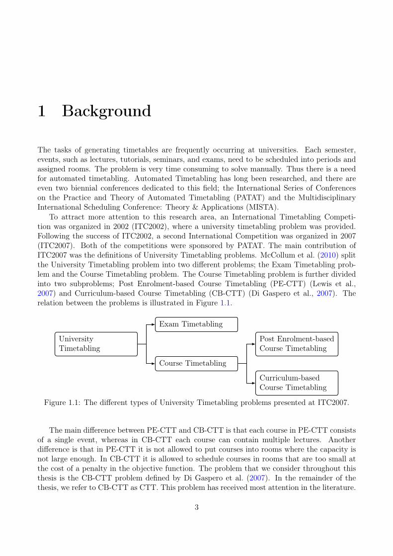
To attract more attention to this research area, an International Timetabling Competi-tion was organized in 2002 (ITC2002), where a university timetabling problem was provided.Following the success of ITC2002, a second International Competition was organized in 2007(ITC2007). Both of the competitions were sponsored by PATAT. The main contribution ofITC2007 was the definitions of University Timetabling problems. McCollum et al. (2010) splitthe University Timetabling problem into two different problems; the Exam Timetabling prob-lem and the Course Timetabling problem. The Course Timetabling problem is further dividedinto two subproblems; Post Enrolment-based Course Timetabling (PE-CTT) (Lewis et al.,2007) and Curriculum-based Course Timetabling (CB-CTT) (Di Gaspero et al., 2007). Therelation between the problems is illustrated in Figure 1.1.

UniversityTimetabling

Exam Timetabling

Course Timetabling

Post Enrolment-basedCourse Timetabling

Curriculum-basedCourse Timetabling

Figure 1.1: The different types of University Timetabling problems presented at ITC2007.

The main difference between PE-CTT and CB-CTT is that each course in PE-CTT consistsof a single event, whereas in CB-CTT each course can contain multiple lectures. Anotherdifference is that in PE-CTT it is not allowed to put courses into rooms where the capacity isnot large enough. In CB-CTT it is allowed to schedule courses in rooms that are too small atthe cost of a penalty in the objective function. The problem that we consider throughout thisthesis is the CB-CTT problem defined by Di Gaspero et al. (2007). In the remainder of thethesis, we refer to CB-CTT as CTT. This problem has received most attention in the literature.

3

One of the reasons for the popularity of this problem is that a website was created as a result ofthe competition (The Scheduling and Timetabling Research Group at the University of Udine,Italy, 2015). This website has made it possible for researchers to upload instances and compareresults.

Most of the research that considers these problems focus on heuristic implementations.The drawback of the heuristics is that they are often problem-specific and do not provide anyguarantee of optimality. So provided a solution from a heuristic it is unknown how far fromoptimality it is unless the optimal solution or a lower bound is known in advance (assumingthat it is a minimization problem). If a heuristic is 5% away from optimality, then this may beconsidered as acceptable, but if the heuristic, for instance, is 60% away from optimality, thenmaybe the implementation of the heuristic should be reconsidered.

Optimal solutions can often be difficult to obtain o that lower bounds can be used instead.However, the quality of the lower bounds is important. For instance, when this Ph.D. projectstarted in 2014, the gap for one of the data instances from ITC2007 between the best-knownsolution and the best-known lower bound was more than 65%. This large gap makes theheuristic appear poor in performance, but this is not necessarily the case. During the work forthis thesis, we improved the lower bound for that particular instance such that the gap for thesame solution is decreased to approximately 15%. Therefore, we focus on methods that eithersearch for the optimal solutions or at least provide lower bounds so the quality of heuristicscan be verified.

In the following section 1.1 we describe CTT in details, and in section 1.2 we provide anoutline for the thesis. We assume that the reader is familiar with Mixed Integer Programming(MIP) and Operations Research in general.

1.1 Curriculum-based Course Timetabling

In this section, we describe the CTT problem as defined by Di Gaspero et al. (2007) andMcCollum et al. (2010) for ITC2007. We are provided with the following; courses, days, timeslots, lecturers, rooms, and curricula. Each course is taught by exactly one lecturer, andcontains lectures that must all be scheduled in a weekly timetable and assigned rooms. Theweek is divided into days and each day is divided into time slots which are all equal in size.We refer to a day and time slot pair as a period, so the total number of periods is the numberof days multiplied by the number of time slots. The length of one lecture corresponds to oneperiod. A curriculum is a set of courses where for every pair there is a set of students attendingboth courses. Furthermore, we are given a set of hard and soft constraints. The weekly scheduleand assignment to rooms must fulfill all the hard constraints, which are as follows:

Lectures (L): Every lecture must be scheduled in a period. If two lectures correspond tothe same course, then they must be scheduled in different periods. If a lecture is notscheduled, then it is counted as one violation, and if two lectures of the same course arescheduled in the same period, then this is also counted as one violation.

Availability (A): A course can have specific periods defined as unavailable periods. If alecture from the course is scheduled in an unavailable period, then this is counted as oneviolation.

4

Conflicts (C): If two courses are taught by the lecturer of if they belong to the same curricu-lum, then they cannot have lectures scheduled in the same periods.

Room Occupancy (RO): Every room cannot accommodate more than one lecture in anyperiod. If more than one lecture fulfill in the same room and same period, then thisconstraint is violated by the number of lectures, minus one.

The problem contains the following four soft constraints, where the goal is to minimize theviolations:

Room Capacity (RC): We are allowed to schedule any course into any room. However, itis desired to be able to accommodate as many students as possible when scheduling thecourses into rooms. Every room has a capacity, i.e., the number of students that the roomcan accommodate. If a course is assigned to a room and the number of students attendingis larger than the capacity of the room, then the violation is one for each student morethan the capacity.

Room Stability (RStab): As the courses contain multiple lectures, it can also be an advan-tage that the lectures are all scheduled in the same room during the week. For everycourse, the violation is one for every distinct room that the course is assigned to, minusone.

Minimum Working Days (MWD): For every course, it is preferred to spread the lecturesacross a predetermined number of days. This number is called minimum working days.If the lectures are scheduled in fewer days than the minimum working days, then theviolation is one for each day below the minimum working days that the lectures arescheduled.

Isolated Lectures (IL): If two periods belong to the same day and are in consecutive timeslots, then we say that the periods are adjacent. Consider some curriculum and somecourse belonging to the curriculum. If the course has a lecture scheduled in a period andno lecture from any of the courses belonging to the curriculum has a lecture scheduled inan adjacent illustrate, then we say that the lecture is isolated. For every curriculum, theviolation is one for every isolated lecture.

Note that the IL constraint is usually referred to as the curriculum compactness constraint inthe literature. We use the name isolated lectures as Bonutti et al. (2012) mentions different waysof defining curriculum compactness and they use the name isolated lectures for the formulationused here and in ITC2007.

Any feasible timetable must fulfil all the hard constraints, i.e., a timetable is consideredfeasible if, and only if, all the hard constraints have no violations. The objective is then to finda feasible timetable while minimizing the soft constraints. Each soft constraint has a weightassociated such that a single-objective is defined by a weighted sum of all the violated softconstraints.

Burke et al. (2010a) show that fulfilling the hard constraints is NP-complete, which meansthat the overall problem is NP-hard. Empirical studies also illustrate that the models are hardto solve, even within hours of computational time.

5

To get an idea of what makes this problem hard to solve, we have tested a MIP modelfrom the paper in chapter 4 without the IL constraints. We used Gurobi provided by GurobiOptimization, Inc. (2016) for these tests. In Table 1.1 we report the results for 21 data instances,which were provided for ITC2007. The first column is the data instance, which is followed bythe best-known upper bounds (UB) for CTT. The next three columns (B & B) report theresults from solving the model when the constraints IL are removed. The first column (Time)reports the running time of the MIP solver to find the optimal solution. The second column(Obj) reports the objective value of the optimal solution for the model, which is a lower boundfor CTT. The last column (Gap) is the gap between the objective value and the best-knownupper bound for CTT. The last six columns report the statistics of the fractionality of the LPrelaxation of the models. We define the fractionality as the number of integer variables thatare fractional in the optimal solution to the LP relaxation. In the first three columns (Allvariables) we report the number for all the variables in the models. Since the Isolated Lectures(IL) is specific for the time schedule, we also consider the fractionality of the time schedule.For each course and each period, we add all the variables together that schedules the course inthat period. If a course in a specific period is scheduled in one room by 0.3 and some otherroom in the same period by 0.4, then we sum this together, so the course is scheduled in theperiod by 0.7 in total, and we consider this as a single variable. In the last three columns (Timevariables) we report the fractionality of all these aggregated variables. For both (All variables)and (Time variables) we report the fractionality when IL is not included in the model (w/oIL) and when IL is included in the model (w/ IL). In the column (Incr.) we report by howmuch the inclusion of the IL constraints increases the number of fractional variables.

In Table 1.1 we see that the model can be solved within minutes when IL is not included.A reason for this can be because of the fractionality of the models since the Branch & Boundalgorithm must branch whenever the integer variables are fractional. We see that including ILincreases the number of all fractional variables more than four times on average, and for the(Time variables) the increase is more than eight times. The gap between the objective values ofthe model without IL and the best-known upper bounds for CTT also illustrate by how muchthe IL constraints impact the objective value.

The problem as it has been presented here is the problem we are considering throughout theentire thesis. However, we briefly present some extensions described byMcCollum et al. (2010)and Bonutti et al. (2012) that could be included to cover a broader variety of universities.These could be either soft or hard and include:

Student Lunch Break: The students should not have a lecture scheduled in at least one timeslot around lunch time.

Windows: If two lectures from the same curriculum are scheduled on the same day, and nolectures are scheduled in the time slots between them, then this is referred to as a window.The penalty for these could depend on the lengths of the windows.

Student Min/Max Load: A minimum (or maximum) number of lectures that the studentsshould be scheduled on any day could be specified. If at least one lecture is scheduledon a day and the total number of lectures is below the minimum (above the maximum),then this could be penalized.

6

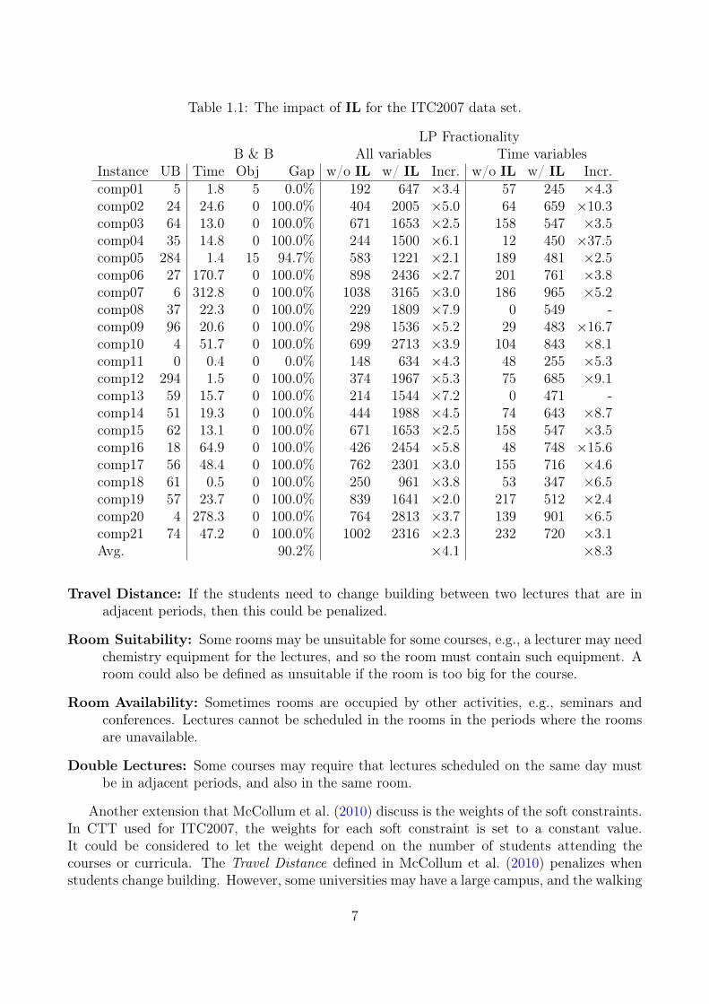
Table 1.1: The impact of IL for the ITC2007 data set.

LP FractionalityB & B All variables Time variables

Instance UB Time Obj Gap w/o IL w/ IL Incr. w/o IL w/ IL Incr.comp01 5 1.8 5 0.0% 192 647 ×3.4 57 245 ×4.3comp02 24 24.6 0 100.0% 404 2005 ×5.0 64 659 ×10.3comp03 64 13.0 0 100.0% 671 1653 ×2.5 158 547 ×3.5comp04 35 14.8 0 100.0% 244 1500 ×6.1 12 450 ×37.5comp05 284 1.4 15 94.7% 583 1221 ×2.1 189 481 ×2.5comp06 27 170.7 0 100.0% 898 2436 ×2.7 201 761 ×3.8comp07 6 312.8 0 100.0% 1038 3165 ×3.0 186 965 ×5.2comp08 37 22.3 0 100.0% 229 1809 ×7.9 0 549 -comp09 96 20.6 0 100.0% 298 1536 ×5.2 29 483 ×16.7comp10 4 51.7 0 100.0% 699 2713 ×3.9 104 843 ×8.1comp11 0 0.4 0 0.0% 148 634 ×4.3 48 255 ×5.3comp12 294 1.5 0 100.0% 374 1967 ×5.3 75 685 ×9.1comp13 59 15.7 0 100.0% 214 1544 ×7.2 0 471 -comp14 51 19.3 0 100.0% 444 1988 ×4.5 74 643 ×8.7comp15 62 13.1 0 100.0% 671 1653 ×2.5 158 547 ×3.5comp16 18 64.9 0 100.0% 426 2454 ×5.8 48 748 ×15.6comp17 56 48.4 0 100.0% 762 2301 ×3.0 155 716 ×4.6comp18 61 0.5 0 100.0% 250 961 ×3.8 53 347 ×6.5comp19 57 23.7 0 100.0% 839 1641 ×2.0 217 512 ×2.4comp20 4 278.3 0 100.0% 764 2813 ×3.7 139 901 ×6.5comp21 74 47.2 0 100.0% 1002 2316 ×2.3 232 720 ×3.1Avg. 90.2% ×4.1 ×8.3

Travel Distance: If the students need to change building between two lectures that are inadjacent periods, then this could be penalized.

Room Suitability: Some rooms may be unsuitable for some courses, e.g., a lecturer may needchemistry equipment for the lectures, and so the room must contain such equipment. Aroom could also be defined as unsuitable if the room is too big for the course.

Room Availability: Sometimes rooms are occupied by other activities, e.g., seminars andconferences. Lectures cannot be scheduled in the rooms in the periods where the roomsare unavailable.

Double Lectures: Some courses may require that lectures scheduled on the same day mustbe in adjacent periods, and also in the same room.

Another extension that McCollum et al. (2010) discuss is the weights of the soft constraints.In CTT used for ITC2007, the weights for each soft constraint is set to a constant value.It could be considered to let the weight depend on the number of students attending thecourses or curricula. The Travel Distance defined in McCollum et al. (2010) penalizes whenstudents change building. However, some universities may have a large campus, and the walking

7

distances between the rooms must be taken into account, which is the case at the TechnicalUniversity of Denmark (Bærentsen, 2012).

1.1.1 Previous Work

In this section, we describe approaches from the literature that has considered CTT. Theresearch on university timetabling problems has, in general, focused on heuristics (Phillips etal., 2015). This focus is also apparent in the overview provided by Bettinelli et al. (2015) andthe survey by Pillay (2016).

As MIP solvers are increasing in performance, so is the interest in applying MIP basedmethods for university timetabling problems (Phillips et al., 2015). As we consider exact andlower bounding methods we provide a brief overview of articles in the literature that considereither exact or lower bounding methods.

Burke et al. (2010a) introduces an exact MIP model of CTT. They formulate the IL byusing a variable for each curriculum and each period. Burke et al. (2008) remove those variablesand instead they have just one variable for each curriculum and each day. The value of thisvariable is then calculated by adding exponentially many constraints. In Burke et al. (2012)they add a subset of the beforementioned constraints and then add the remaining dynamicallywhenever they are violated. Burke et al. (2010b) takes the model from Burke et al. (2010a) andsplit it into two stages. The first stage is to schedule the courses into the periods, i.e., ignore theroom assignments. However, it is ensured that the time schedule is feasible by not schedulingmore lectures in any period than the number of rooms available. In the second stage, they takethe period schedule and fix the model either completely or partially to the selected periods andthen solve the full model. This approach is executed iteratively.

Splitting the problem into two stages is also considered by Lach and Lübbecke (2008) andLach and Lübbecke (2012), where the problem is also split into two stages; the first stage createsthe time schedule and the second stage makes the room assignment given the time schedule.Lach and Lübbecke (2012) also show how the RC constraints can be added to the first stageproblem by grouping the rooms together according to their capacities. Then the first stageproblem schedules the courses into periods and capacities.

Hao and Benlic (2011) considers the first stage problem of Lach and Lübbecke (2012). Theymake a decomposition by relaxing some of the constraints such that the problem can be dividedinto subproblems. They then compute a lower bound for each subproblem and sum them upto get a lower bound for the overall problem.

Cacchiani et al. (2013) also compute lower bounds. They do this by splitting the probleminto two parts where one part considers the constraints MWD and IL and the other partconsiders the constraints RC and RStab. A lower bound is then calculated by summing uplower bounds for the two parts. The part which considers the constraints MWD and IL canbe time-consuming to solve. So they apply a Dantzig-Wolfe decomposition of their model suchthat the pricing problem is decomposable by days and solve the model by column generation.

Asín Aschá and Nieuwenhuis (2014) proposes multiple satisfiability encodings. They start offby treating the soft constraints as hard constraints and solve the problem as a pure satisfiabilityproblem. Then they relax the constraints one by one and move towards a weighted partialmaximum satisfiability encoding.

8

In the paper in chapter 4 we provide more details on some of the methods from the literature.For an even more comprehensive overview of the literature regarding CTT, we refer to Bettinelliet al. (2015).

1.2 Thesis OutlineThis thesis is divided into three main parts; Part I Introduction, Part II Exact Methods andPart III Lower Bounding Methods. Part I is the introduction to the thesis and covers thedescription of the problem, the scientific contributions and the conclusions of the work. Inchapter 1 we provide the description of the problem that has been considered throughout thework for this thesis, and related work that has been applied. In chapter 2 we summarize thescientific contributions and the conclusion of the work for this thesis. Furthermore, we providesuggestions for future research. The last chapter 3 of part I is a summary of all 15 differentapproaches that we have implemented and tested during the work for this thesis. The chapteris not necessary to read but is included for the readers that are interested in the details of allthe approaches that we have implemented. Part II and part III constitute the majority of thethesis, and both consist of two articles. The articles in part II focuses on exact methods, andthe articles in part III focuses on lower bounding methods.

9

2 Scientific Contributions

The scientific contributions are here summed up for the four papers. All four papers aresubmitted to international peer-reviewed journals. The first two papers focus on exact methods.A common approach to solving the problem is to divide it into two parts; a Time Schedulingproblem and a Room Allocation problem. Then the Time Scheduling problem is solved, andthe solution is provided for the Room Allocation problem to generate a complete solution.This approach can be iterated. The drawback of this approach is that we lose the guaranteeof optimality. So the focus in this thesis has been on exact methods in the first two papersand then lower bounding methods in the last two papers. In the following we describe thefour papers. Section 2.1 contains our conclusions of the work conducted for this thesis and insection 2.2 we provide suggestions for future research.

Chapter 4: Flow Formulations for Curriculum-based Course Timetabling This pa-per combines the two components, the Time Scheduling problem and the Room Allocationproblem, into two exact formulations, which are solved by a generic MIP solver. The first for-mulation is based on an underlying minimum cost flow (MIN) problem. The second formulationis based on a multi-commodity flow (MULT) problem. The MIN problem is known to containthe integrality property, and hence being solvable in polynomial time, but the MULT problemis NP-hard in general. However, we proved that it suffices to include the LP-relaxation ofMULT in the model. For both of these formulations, the result is that the number of integervariables is significantly lower than other exact formulations in the literature at the cost ofmany continuous variables.

Compared to other approaches in the literature that provide both lower and upper boundsthe MIN formulation provides the best performance on the data instances from ITC2007. Wealso compared the flow formulations with the basic MIP model which we present in section 3 ona total of 32 instances. The results showed that the reformulations outperform the basic modelboth on the lower and upper bounds. Here the MIN formulation obtained a lower bound whichis at least as good as MULT and the basic model on 28 of the instances, and for 11 of theseinstances, MIN obtained a strictly better bound than the other two. On 24 of the instancesthe MIN formulation obtained an upper which is at least as good as the other two, and for 12of these the upper bound is strictly less than for the other two formulations. Out of the 32instances, six of them are still open. The MIN formulation improved the lower bound of oneof them from 101 to 142. We believe that other approaches from the literature based on thebasic model can benefit from these reformulations.

The MULT formulation was submitted as an extended abstract to the peer-reviewed MISTAconference in 2015 (Bagger et al., 2015). The full paper with both methods is submitted toAnnals of Operations Research and contributes with:

11

• Two new formulations that outperform the basic formulation.

• An improvement of the lower bound for one out of the six instances that are still open bymore than 40%.

Chapter 5: Benders’ Decomposition for Curriculum-based Course Timetabling Inthe previous paper Flow Formulations for Curriculum-based Course Timetabling, two formula-tions were provided for CTT such that a large part of the variables could be relaxed to contin-uous variables. The paper Benders’ Decomposition for Curriculum-based Course Timetablingexpands on one of the formulations by projecting out all these continuous variables. Then aBenders’ Decomposition algorithm is implemented, which is the first time to our knowledge thata full Benders’ Decomposition algorithm is implemented for CTT, i.e., where Benders’ cuts aregenerated dynamically as they are violated. We also implemented a heuristic to generate upperbounds based on solving a series of Minimum Cost Maximum Flow problems as the solutionsproduced inside the decomposition were usually infeasible. The main focus of the heuristic wasto gain feasibility, so we believe that there is a potential here to improve the implementationfurther.

We compared the decomposition with other approaches on a total of 38 real-life instances.Out of these 38 instances, 12 of them are still open, and our implementation improved thelower bound on eight of these instances. Six of the open instances are significantly larger andmore difficult to solve than the other 32. For these six instances our decomposition is thefirst MIP-based approach that has been applied, and the first time lower bounds have beencalculated.

We compared Benders’ Decomposition on the large instances with MULT since no otherMIP-based methods have been applied. These tests illustrated that the benefits of Benders’Decomposition are more apparent for large data instances. Solving the root node LP withMULT had a running time of more than half an hour for three of the instances, and for the threeother instances, the running time was more than one and a half hour. For our decomposition,the longest running time is less than four minutes. On average the speed-up was more than 30times, and the improvements of the lower bounds were 14%. For the upper bounds, MULT wereonly able to obtain a feasible solution for four of the instances, which Benders’ Decompositionimproved by 35% on average. Furthermore, the decomposition was able to obtain solutions forall instances.

The paper is submitted to Computers & Operations Research and contributes with:

• The first Benders’ Decomposition algorithm for CTT.

• First time that the lower bounds are calculated for six large instances.

• Improvement of the lower bounds for eight out of 12 of the real-life instances that are stillopen.

Chapter 6: Daily Course Pattern Formulation and Valid Inequalities for theCurriculum-based Course Timetabling Problem The previous two papers focused onthe improvement of exact methods and provided methods to combine the Time Schedulingproblem and the Room Allocation problem. Empirical studies have shown that the Time

12

Scheduling problem is the most time-consuming problem of the two components. So in thispaper, we focus on the Time Scheduling problem as any improvements on this component canbe applied to the two previous approaches. In the paper, Daily Course Pattern Formulation andValid Inequalities for the Curriculum-based Course Timetabling Problem a pattern formulationis provided. For each course and each day we enumerate all the patterns that are possible forthe course to be assigned on that day. In our model, there is a binary variable for each of thesepatterns for each course and each day.

The benefit of the pattern formulation is that we can preprocess the model to removevariables. We implement multiple preprocessing techniques where one is based on solvingauxiliary maximum flow problems. We also generate valid inequalities, which are difficult toderive for the basic formulation. Some of these inequalities come from generating a conflictgraph for the variables, and we show how this graph can be constructed by extending thepreprocessing techniques. We discuss in the paper that one of the benefits of the patternformulation is that it is more flexible regarding adding additional constraints or penalties thanthe basic model.

We compared the formulation to other lower bounding approaches from the literature on21 real-life instances from ITC2007, and show that the pattern formulation has a better per-formance. Four of the instances are still open, and our formulation improves the lower boundof three of them. The paper is submitted to Journal of Scheduling and contributes with:

• A new lower bounding formulation of CTT that outperforms other approaches from theliterature.

• Implementation of novel preprocessing and clique graph generation techniques.

• Improvements of the best-known lower bound for three out of the four real-life instancesthat are still open.

Chapter 7: Dantzig-Wolfe Decomposition of the Daily Pattern Formulation forCurriculum-based Course Timetabling Dantzig-Wolfe Decomposition has been appliedto CTT before. However, they are all based on the basic formulation. As a stronger formulationis provided in the previous paper Daily Course Pattern Formulation and Valid Inequalities forthe Curriculum-based Course Timetabling Problem, then we use this formulation for the decom-position. We apply the decomposition such that there is a pricing problem for each day andwe solve the LP-relaxation of the master problem by Column Generation. The decompositionputs the formulation of the isolated lectures into the pricing problems, which is an advantageas it was shown in section 1.1 that these soft constraints are the ones that are most difficult.

We provide a preprocessing technique that can be applied in an iteration of the ColumnGeneration algorithm and also show how the technique can be extended to generate inequalities.The empirical study shows that our preprocessing implementation can remove almost half ofthe variables from the model on average. Applying this technique to other scheduling problemscould be interesting.

We implement a Local Branching algorithm to solve the pricing problems by using previouslygenerated columns. To the best of our knowledge, this is the first time Local Branching isimplemented in a pricing problem in Column Generation, though the nature of the ColumnGeneration algorithm fits perfectly with Local Branching. As Local Branching is a general

13

framework and easy to implement it can be considered for other problems solved by ColumnGeneration as well. We show that more than 90% of the time of the Column Generationalgorithm is spent in the pricing problems. So we suggest any future research, to focus onimproving the running time of the pricing problems.

We compared the decomposition to other approaches from the literature. The lower boundsobtained are higher than for most other approaches except for the pattern formulation in theprevious paper. However, for the four instances from ITC2007 that are still open we obtain ahigher lower bound for all of them, which decreases the average gap to the best-known upperbounds from 24% to 11%. The paper is submitted to European Journal of Operational Researchwith the following contributions:

• A new Dantzig-Wolfe Decomposition and Column Generation algorithm for CTT.

• Novel preprocessing and inequality generation for the pricing problem.

• The first time Local Branching is applied in a pricing problem inside a Column Generationalgorithm.

• Improvements of the best-known lower bounds for all four real-life instances from ITC2007that are still open.

2.1 ConclusionDue to the second international timetabling competition in 2007 (ITC2007), the Curriculum-based Course Timetabling (CTT) problem has received a lot of attention. The CTT problemconsists of assigning courses into periods and rooms. For University Timetabling problems,in general, most literature has focused on heuristic applications which are also apparent inthe different surveys. The heuristics are attractive in real-world settings as they are usuallyfast. The drawback of the heuristics is that they are problem-specific and do not provideinformation on how far they are from optimality. For the competition 21 data instances wereprovided where four of them are still open, meaning that for these four instances, the best-known lower bounds do not equal the best-known upper bounds. The objective of this thesishas been to minimize the gap between the best-known upper bounds and the best-known lowerbounds for CTT by using Mixed Integer Programming (MIP). A total of 15 different MIP basedformulation and methodologies have been implemented and tested during this work. Four ofthese implementations led to article submissions for peer-reviewed international journals.

Most of the MIP-based approaches in the literature split the problem into two components;a Time Scheduling problem and a Room Allocation problem. The Time Scheduling problemconsists of scheduling the course into periods, and the Room Allocation problem assigns coursesto rooms. The Time Scheduling problem is commonly solved first, and the solution is then pro-vided to the Room Allocation problem. The first article we submitted focused on combiningthe two components into one model. Two formulations were provided that improved the perfor-mance of a generic MIP solver, both regarding the lower and upper bounds. The second articleexpanded on the results from the first article by applying a Benders’ Decomposition on one ofthe provided formulations. The results showed improvements on the lower bounds compared toliterature. The method was also tested on six large data instances where MIP based approaches

14

have not been applied before. On these instances, the decomposition improved the performanceof the MIP solver significantly on both the lower and upper bounds.

The last two articles focused on improving the lower bounds by considering the TimeScheduling problem as empirical studies in literature have shown that this is the most time-consuming part. In the first of the two articles, a pattern formulation is implemented byenumerating all possible patterns for each course and each day. The pattern formulation pro-vided stronger lower bounds compared to the literature. In the last article, we expanded onthe pattern formulation by applying a Dantzig-Wolfe Decomposition of the model and solvedit by Column Generation. The benefit of the decomposition was that the formulation of someof the hardest soft constraints was put into the pricing problems, which are smaller and easierto solve. The decomposition further improved the bounds for the four instances from ITC2007that are still open.

The articles in this thesis have brought us closer to the goal of closing the gap betweenthe best-known upper and lower bounds for CTT. Though CTT was the problem in focus, themethods implemented here are general enough to be applied for other scheduling problems.

2.2 Future Research

We have implemented and tested different MIP based approaches on CTT, leading to foursubmitted articles. In chapter 3 we describe additional implementations that we have tested,which were not all successful for CTT. In total, we report 15 different formulations, methodsand implementations. This vast amount of implementations shows how difficult this problemis, and that further research is needed. The theory and notes on the implementations areprovided, and it could be interesting to see if other scheduling problems can benefit from theseapproaches, or which changes to the methods that are needed for them to be successful forCTT.

Other suggestions for future research is to improve the approaches from our submittedarticles. In the second article, we consider a Benders’ Decomposition. We implemented aheuristic to obtain feasible solutions but saw that our implementation did not improve theupper bounds. The focus of the heuristic was to obtain a feasible solution by assigning roomsprovided that the time schedule was feasible. Therefore, we suggest considering implementinga heuristic which also considers improving the solutions, for instance by also making changesto the time schedule. In the last article, we applied a Dantzig-Wolfe Decomposition. For someof the instances that we tested the implementation of the Column Generation algorithm wastoo time-consuming to be embedded in a full Branch & Price algorithm. As more than 90% ofthe running time was spent in the pricing problems we suggest that solution methods for theseproblems are researched further.

Some methods that we have briefly tested for the pricing problems include Dynamic Pro-gramming, Constraint Programming, Lagrangian Relaxation and Benders’ Decomposition.However, we have not studied these implementations enough for us to draw conclusions, whichis why we have not included them in the description of the implemented approaches. Anotherinteresting study could be to consider why some of the instances are significantly more timeconsuming than others, for instance by examining the feature space suggested by Smith-Mileset al. (2014). This information could be useful in the development of solution approaches.

15

When the pricing problems can be solved in a reasonable amount of time, we would liketo see the Benders’ Decomposition algorithm included in the Dantzig-Wolfe Decomposition.One way to include Benders’ Decomposition could be to solve the room allocation problemin another pricing problem and then add the Benders’ feasibility cuts in the master problemto connect the pricing problems. Another possibility is to use the current implementation asthe lower bounding problem in a Branch & Price algorithm and apply branching rules on thetime schedule. Then switch to the Benders’ Decomposition algorithm for nodes that are deepenough in the search tree.

16

3 Implemented Approaches

In this chapter we provide an overview of all the methods that has been tested during this workfor the CTT problem. Not all methods have been equally successful. However, the knowledge isuseful for the timetabling community to get an overview of methods that are either successful,should be avoided or needs further research. Furthermore, even though some of the approacheshave not been successful for CTT, it could be interesting to see if other scheduling or timetablingproblems can benefit from these methods. Before describing all the approaches that have beentested, we first provide a basic (MIP) model of the problem. All the tested methods refer tothis model as the basis.

The set of courses is denoted C. For each course c ∈ C, the number of lectures to bescheduled is denoted as Lc. For the periods we have the set of days, D, and the set of timeslots, T . For each course c ∈ C, day d ∈ D and time slot t ∈ T we let the parameter Fc,d,t takevalue one if the course is available in the specific period, and zero otherwise. The set of roomsis denoted R. We let xc,d,t,r be a binary variable taking value one if course c ∈ C is scheduled onday d ∈ D in time slot t ∈ T in room r ∈ R, and zero otherwise. To ensure that the constraintL is not violated we sum over all the binary variables associated with one course and add aconstraint that the sum must equal Lc:∑

d∈D,t∈T ,r∈R

xc,d,t,r = Lc, ∀c ∈ C (3.1)

This constraint only ensures that all lectures are scheduled, but not that they are scheduledin different time slots. We ensure this by the following constraints, where we also include theA constraint: ∑

r∈R

xc,d,t,r ≤ Fc,d,t, ∀c ∈ C, d ∈ D, t ∈ T (3.2)

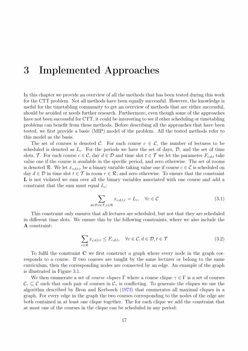
To fulfil the constraint C we first construct a graph where every node in the graph cor-responds to a course. If two courses are taught by the same lecturer or belong to the samecurriculum, then the corresponding nodes are connected by an edge. An example of the graphis illustrated in Figure 3.1.

We then enumerate a set of course cliques Γ where a course clique γ ∈ Γ is a set of coursesCγ ⊆ C such that each pair of courses in Cγ is conflicting. To generate the cliques we use thealgorithm described by Bron and Kerbosch (1973) that enumerates all maximal cliques in agraph. For every edge in the graph the two courses corresponding to the nodes of the edge areboth contained in at least one clique together. The for each clique we add the constraint thatat most one of the courses in the clique can be scheduled in any period:

17

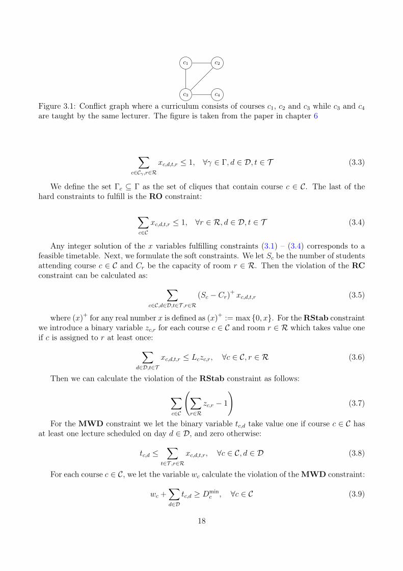
c1 c2

c3 c4

Figure 3.1: Conflict graph where a curriculum consists of courses c1, c2 and c3 while c3 and c4

are taught by the same lecturer. The figure is taken from the paper in chapter 6

∑c∈Cγ ,r∈R

xc,d,t,r ≤ 1, ∀γ ∈ Γ, d ∈ D, t ∈ T (3.3)

We define the set Γc ⊆ Γ as the set of cliques that contain course c ∈ C. The last of thehard constraints to fulfill is the RO constraint:

∑c∈C

xc,d,t,r ≤ 1, ∀r ∈ R, d ∈ D, t ∈ T (3.4)

Any integer solution of the x variables fulfilling constraints (3.1) – (3.4) corresponds to afeasible timetable. Next, we formulate the soft constraints. We let Sc be the number of studentsattending course c ∈ C and Cr be the capacity of room r ∈ R. Then the violation of the RCconstraint can be calculated as: ∑

c∈C,d∈D,t∈T ,r∈R

(Sc − Cr)+ xc,d,t,r (3.5)

where (x)+ for any real number x is defined as (x)+ := max {0, x}. For theRStab constraintwe introduce a binary variable zc,r for each course c ∈ C and room r ∈ R which takes value oneif c is assigned to r at least once:∑

d∈D,t∈T

xc,d,t,r ≤ Lczc,r, ∀c ∈ C, r ∈ R (3.6)

Then we can calculate the violation of the RStab constraint as follows:

∑c∈C

(∑r∈R

zc,r − 1

)(3.7)

For the MWD constraint we let the binary variable tc,d take value one if course c ∈ C hasat least one lecture scheduled on day d ∈ D, and zero otherwise:

tc,d ≤∑

t∈T ,r∈R

xc,d,t,r, ∀c ∈ C, d ∈ D (3.8)

For each course c ∈ C, we let the variable wc calculate the violation of the MWD constraint:

wc +∑d∈D

tc,d ≥ Dminc , ∀c ∈ C (3.9)

18

The set of curricula is denoted Q, and for each curriculum q ∈ Q the set of courses belongingto q is denoted Cq ⊆ C. Similarly, we let the set of curricula that course c ∈ C belongs to bedenoted as Qc. For each curriculum q ∈ Q, day d ∈ D and time slot t ∈ T we let the binaryvariable sq,d,t take value one if q has an isolated lecture at day d in time slot t, and zerootherwise. For t ∈ T we denote the time slot that is right before as t − 1 and we denote thetime slot right after t as t+ 1. For ease of notation, we define xq,d,t for each curriculum q ∈ Q,day d ∈ D and time slot t ∈ T as follows:

xq,d,t :=∑

c∈C,r∈R

xc,d,t,r, ∀q ∈ Q, d ∈ D, t ∈ T (3.10)

If t is the first time slot then we define xq,d,t−1 to be zero and if t is the last time slot thenwe define xq,d,t+1 to be zero. Then we can calculate the isolated lectures as follows:

sq,d,t ≥ xq,d,t − xq,d,t−1 − xq,d,t+1, ∀q ∈ Q, d ∈ D, t ∈ T (3.11)

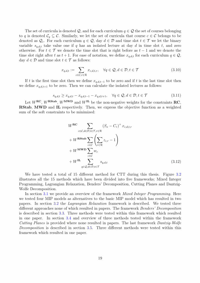
Let WRC, WRStab, WMWD and W IL be the non-negative weights for the constraints RC,RStab, MWD and IL respectively. Then, we express the objective function as a weightedsum of the soft constraints to be minimized:

WRC∑

c∈C,d∈D,t∈T ,r∈R

(Sx − Cr)+ xc,d,t,r

+WRStab∑c∈C

(∑r∈R

zc,r − 1

)+WMWD

∑c∈C

wc

+W IL∑

q∈Q,d∈D,t∈T

sq,d,t (3.12)

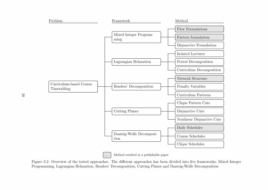
We have tested a total of 15 different method for CTT during this thesis. Figure 3.2illustrates all the 15 methods which have been divided into five frameworks; Mixed IntegerProgramming, Lagrangian Relaxation, Benders’ Decomposition, Cutting Planes and Dantzig-Wolfe Decomposition.

In section 3.1 we provide an overview of the framework Mixed Integer Programming. Herewe tested four MIP models as alternatives to the basic MIP model which has resulted in twopapers. In section 3.2 the Lagrangian Relaxation framework is described. We tested threedifferent approaches none of which resulted in papers. The framework Benders’ Decompositionis described in section 3.3. Three methods were tested within this framework which resultedin one paper. In section 3.4 and overview of three methods tested within the frameworkCutting Planes is provided where none resulted in papers. The last framework Dantzig-WolfeDecomposition is described in section 3.5. Three different methods were tested within thisframework which resulted in one paper.

19

Curriculum-based CourseTimetabling Benders’ Decomposition

Cutting Planes

Lagrangian Relaxation

Mixed Integer Program-ming

Dantzig-Wolfe Decomposi-tion

Pattern formulation

Flow Formulations

Disjunctive Formulation

Period Decomposition

Curriculum Decomposition

Isolated Lectures

Disjunctive Cuts

Clique Pattern Cuts

Nonlinear Disjunctive Cuts

Penalty Variables

Curriculum Patterns

Network Structure

Course Schedules

Clique Schedules

Daily Schedules

MethodFrameworkProblem

... Method resulted in a publishable paper

Figure 3.2: Overview of the tested approaches. The different approaches has been divided into five frameworks; Mixed IntegerProgramming, Lagrangian Relaxation, Benders’ Decomposition, Cutting Planes and Dantzig-Wolfe Decomposition

20

3.1 Mixed Integer Programming

In this section we describe some alternatives to the basic model. We have tested four alternativeformulations to the basic model; two formulations based on underlying flow networks, a patternbased formulation where each pattern corresponds to an entire time schedule for one courseon one day and the last formulation is based on reformulating the modelling of the isolatedlectures. An overview of the flow formulations and the pattern formulation are provided insection 2. A detailed description for the flow formulations is provided in the paper in chapter 4and the details of the pattern formulation is provided in the paper in chapter 6. In the followingsection 3.1.1 we describe how the isolated lectures can be reformulated in a disjunctive model.

3.1.1 Disjunctive Formulation

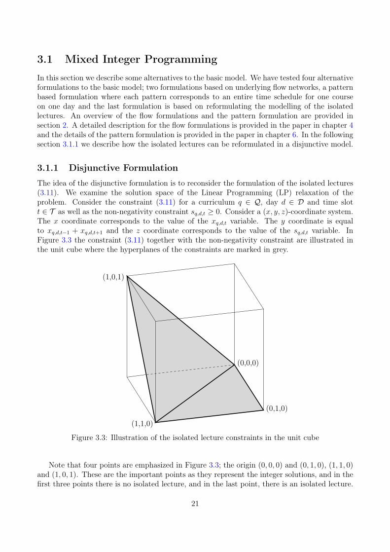
The idea of the disjunctive formulation is to reconsider the formulation of the isolated lectures(3.11). We examine the solution space of the Linear Programming (LP) relaxation of theproblem. Consider the constraint (3.11) for a curriculum q ∈ Q, day d ∈ D and time slott ∈ T as well as the non-negativity constraint sq,d,t ≥ 0. Consider a (x, y, z)-coordinate system.The x coordinate corresponds to the value of the xq,d,t variable. The y coordinate is equalto xq,d,t−1 + xq,d,t+1 and the z coordinate corresponds to the value of the sq,d,t variable. InFigure 3.3 the constraint (3.11) together with the non-negativity constraint are illustrated inthe unit cube where the hyperplanes of the constraints are marked in grey.

(0,0,0)

(1,0,1)

(1,1,0)

(0,1,0)

Figure 3.3: Illustration of the isolated lecture constraints in the unit cube

Note that four points are emphasized in Figure 3.3; the origin (0, 0, 0) and (0, 1, 0), (1, 1, 0)and (1, 0, 1). These are the important points as they represent the integer solutions, and in thefirst three points there is no isolated lecture, and in the last point, there is an isolated lecture.

21

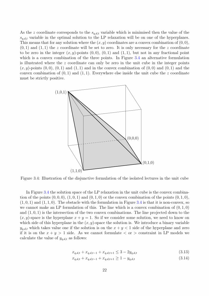
As the z coordinate corresponds to the sq,d,t variable which is minimised then the value of thesq,d,t variable in the optimal solution to the LP relaxation will be on one of the hyperplanes.This means that for any solution where the (x, y) coordinates are a convex combination of (0, 0),(0, 1) and (1, 1) the z coordinate will be set to zero. It is only necessary for the z coordinateto be zero in the integer (x, y)-points (0, 0), (0, 1) and (1, 1), but not in any fractional pointwhich is a convex combination of the three points. In Figure 3.4 an alternative formulationis illustrated where the z coordinate can only be zero in the unit cube in the integer points(x, y)-points (0, 0), (0, 1) and (1, 1) and in the convex combination of (0, 0) and (0, 1) and theconvex combination of (0, 1) and (1, 1). Everywhere else inside the unit cube the z coordinatemust be strictly positive.

(0,0,0)

(1,0,1)

(1,1,0)

(0,1,0)

Figure 3.4: Illustration of the disjunctive formulation of the isolated lectures in the unit cube

In Figure 3.4 the solution space of the LP relaxation in the unit cube is the convex combina-tion of the points (0, 0, 0), (1, 0, 1) and (0, 1, 0) or the convex combination of the points (0, 1, 0),(1, 0, 1) and (1, 1, 0). The obstacle with the formulation in Figure 3.4 is that it is non-convex, sowe cannot make an LP formulation of this. The line which is a convex combination of (0, 1, 0)and (1, 0, 1) is the intersection of the two convex combinations. The line projected down to the(x, y)-space is the hyperplane x+ y = 1. So if we consider some solution, we need to know onwhich side of this hyperplane in the (x, y)-space the solution is. We introduce a binary variableyq,d,t which takes value one if the solution is on the x + y < 1 side of the hyperplane and zeroif it is on the x + y > 1 side. As we cannot formulate < or > constraint in LP models wecalculate the value of yq,d,t as follows:

xq,d,t + xq,d,t−1 + xq,d,t+1 ≤ 3− 2yq,d,t (3.13)xq,d,t + xq,d,t−1 + xq,d,t+1 ≥ 1− yq,d,t (3.14)

22

If the point is on the x + y < 1 side of the hyperplane in the (x, y)-space then we use thehyperplane spanned by the three points (0, 0, 0), (1, 0, 1) and (0, 1, 0); x− z = 0. If the point ison the x+ y > 1 side of the hyperplane in the (x, y)-space then we use the hyperplane spannedby the three points (0, 1, 0), (1, 0, 1) and (1, 1, 0); y + z = 1. In an LP model this can beformulation as follows:

sq,d,t ≥ xq,d,t + yq,d,t − 1 (3.15)sq,d,t ≥ 1− yq,d,t − xq,d,t−1 − xq,d,t+1 (3.16)sq,d,t ≥ 0 (3.17)

If yq,d,t = 1 then constraint (3.15) is activated and (3.16) becomes inactive and oppositefor yq,d,t = 0. Note that for any point that is on the hyperplane x + y = 1 then yq,d,t can beeither zero or one. However, as we know that the variables xq,d,t, xq,d,t−1 and xq,d,t+1 then wecan formulate the following disjunction of the model:{

xq,d,t + xq,d,t−1 + xq,d,t+1 ≤ 1

sq,d,t ≥ xq,d,t

} ∨ {xq,d,t + xq,d,t−1 + xq,d,t+1 ≥ 2

}(3.18)

The disjunction (3.18) corresponds to replacing the right-hand side of (3.14) by 2− 2yq,d,t.Introducing this disjunction makes constraint (3.16) redundant as there can only be an isolatedlecture in the left branch, i.e., when yq,d,t = 1. The disjunction (3.18) also means that weimplicitly minimize the value of yq,d,t which makes the constraint (3.13) redundant, thus thedisjunctive formulation is as follows:

xq,d,t + xq,d,t−1 + xq,d,t+1 + 2yq,d,t ≥ 2 (3.19)xq,d,t + yq,d,t−sq,d,t ≤ 1 (3.20)

sq,d,t ≥ 0 (3.21)

The downside about the formulation (3.19) – (3.21) is that it requires O (|Q||D||T |) extrabinary variables. Another downside is that the LP relaxation is weaker compared to the LPrelaxtion of the basic model. If xq,d,t + xq,d,t−1 + xq,d,t+1 is at least two then both of theformulations does not provide a higher lower bound for sq,d,t than zero. We assume that thesum is less than two and isolate yq,d,t in (3.19):

yq,d,t ≥ 1− 1

2(xq,d,t − xq,d,t−1 − xq,d,t+1) (3.22)

As we minimize yq,d,t then it will be equal to the right-hand side of (3.22) and we insert thisin (3.20):

sq,d,t ≥1

2(xq,d,t − xq,d,t−1 − xq,d,t+1) (3.23)

Here we see that in the LP relaxation, the isolated lectures are only penalised in the disjunc-tive formulation by half of what they are penalised by the original formulation. The disjunctiveformulation also resulted in a poorer performance than the original formulation when we tested

23

it in the commercial MIP solvers such as Gurobi by Gurobi Optimization Inc. (2015) andCPLEX by International Business Machines Corp. (2017). CPLEX provides the user with thecapability of implementing custom branching decisions. So to get around the issues of the dis-junctive formulation, we implemented a custom branching decision in CPLEX inspired by thedisjunctive formulation. The idea is to provide CPLEX with the original formulation, i.e., withthe formulation of the isolated lectures in (3.11). A common branching decision is to choose aninteger variable x with a fractional value x in the LP relaxation and then apply the branching:

x ≤ bxc ∨ x ≥ dxe (3.24)

Instead of choosing one variable for the branching decision, we consider a sum xq,d,t +xq,d,t−1 + xq,d,t+1. We then compute the penalty of the isolated lecture using the disjunctiveformulation. If the value of the disjunctive formulation is greater than sq,d,t then the sum isa candidate for the branching decision, other we let CPLEX decide on the branching. If thissum is between one and two, then we apply the branching from the disjunction in (3.18). Ifthe sum is between zero and one, then we apply the branching in (3.25). If the sum is equal toone, then we pick one of the two branching decisions randomly.

{xq,d,t + xq,d,t−1 + xq,d,t+1 ≤ 0

} ∨ {xq,d,t + xq,d,t−1 + xq,d,t+1 ≥ 1

sq,d,t ≥ 1− xq,d,t−1 − xq,d,t+1

}(3.25)

The question left to answer is which sum to choose. When branching on a single variables,then a common approach is to pick the variable which is most fractional, i.e., if bxe is the valuex rounded to the nearest integer then we pick the variable which maximizes |x − bxe|. Thisbranching rule means that we branch on the variable that violates the integrality requirementthe most. We do something similar for the calculation of the isolated lectures. Considercurriculum q ∈ Q, day d ∈ D and time slot t ∈ T . Let sLPq,d,t be the value of the variablesq,d,t calculated in the optimal solution of the LP relaxation using the constraints (3.11) andsq,d,t ≥ 0. We calculate the sum xq,d,t + xq,d,t−1 + xq,d,t+1. If the sum is less than or equal toone, then the disjunctive value sDisjunctq,d,t of the variable sq,d,t is set to xq,d,t. If the sum is greaterthan one and less than two, then we set sDisjunctq,d,t = 1 − xq,d,t−1 − xq,d,t+1. In all other caseswe set sDisjunctq,d,t = 0. Note that sDisjunctq,d,t ≥ sLPq,d,t. We then pick the curriculum q ∈ Q, dayd ∈ D and time slot t ∈ T which maximizes sviol := sDisjunctq,d,t − sLPq,d,t. If sviol > 0 we apply thebranching (3.18) or (3.25) depending on the sum as mentioned earlier, otherwise we let CPLEXdecide. The issue we encountered is that when implementing custom branching decisions inCPLEX a lot of the internal features is turned off. So the lower bounds were not as strong aswithout the custom branching, and the heuristics also did not produce solutions which are asgood as the solutions obtained without the custom branching. Therefore, we suggest that anyresearchers that want to study this method further to consider using another framework suchas SCIP (Gamrath et al., 2016) where the user is given more control of the Branch & Boundalgorithm.

24

3.2 Lagrangian RelaxationIn this section we describe different methods that we have tested based on Lagrangian Re-laxation. Before the description of the methods we provide an introduction to LagrangianRelaxation in section 3.2.1. The idea of all the methods tested within this framework is toconsider the formulation of the isolated lectures. In section 3.2.2 we apply the relaxation to thedirect formulation of the isolated lectures. In section 3.2.3 we replace the formulation of theisolated lectures and describe how we apply Lagrangian Relaxation to this reformulation whichresults in a subproblem that is decomposable by the periods. In section 3.2.4 we reformulationthe entire model such that the subproblem is decomposable by the curricula.

3.2.1 Introduction to Lagrangian Relaxation

In this section we provide a brief description of Lagrangian Relaxation similar to the descrip-tion by Martin (1999, chapter 12), which we refer to for a detailed description of LagrangianRelaxation. Consider a MIP problem in the following form:

min c>x

s.t. Ax ≥ b

Bx ≥ d

x ∈ X

(MIP)

The idea of Lagrangian Relaxation is to take a set of the constraints and relax them bymultiplying them with a non-negative vector u, referred to as the Lagrangian multipliers, andinserting them in the objective function:

L(u) = min{

(c−B>u)>x+ d>u |Ax ≥ b, x ∈ X}

(3.26)

We refer to the problem (3.26) as the Lagrangian Subproblem. For a fixed value of u theoptimal solution of the subproblem provides a lower bound for (MIP). The goal is to maximizethis lower bound by solving the following model:

max {L(u) |u ≥ 0} (LR)

We let zMIP and zLP be the objective values of the optimal solution of (MIP) and the LPrelaxation of the model respectively. Furthermore, we let zLR be the objective value of theoptimal solution to (LR), and we have the following relation

zLP ≤ zLR ≤ zMIP (3.27)

If the model (3.26) contains the integrality property, i.e., that the extreme points of theLP-relaxation are all integral, then zLP = zLR. So the set of constraints to relax should beselected such that the subproblem does not contain the integrality property. However, theconstraints should also be selected such that the resulting subproblem is easier to solve thanthe original problem. Different methods can be applied to solve the problem (LR). Onemethod is Subgradient Search. This algorithm is an iterative procedure which starts by settingthe Lagrangian multipliers to some initial value, e.g., zero. Then the optimal solution of thesubproblem (3.26) is found for these values of u. Let uj be the value in the j′th iteration of

25

the subgradient search and let xj be the optimal solution to the subproblem for uj. Thend − Bxj is a subgradient vector of the subproblem for uj and for a scalar αj > 0 we calculatethe multipliers for the next iteration as follows:

uj+1 = max{

0, uj + αj(d−Bxj

)}(3.28)

We let L be an upper bound on the value of the optimal solution to the Lagrangian Relax-ation. This upper bound can for instance by the objective value of some feasible solution tothe original model MIP. For a positive scalar θj between zero and two, the choice of αj can bedetermined by:

αj =θj(L− L (uj)

)‖d−Bxj‖2

(3.29)

The value of θj can for instance be set to two in the first iteration and then halved wheneverthe lower bound has not improved for some number of iterations. We refer to Martin (1999,section 12.5) for descriptions of other methods to solve the Lagrangian Relaxation.

3.2.2 Isolated Lectures

The idea in this section is to relax the constraints (3.11) using as it was shown in section 1.1that the problem is much easier to solve without these constraints. For each curriculum q ∈ Q,day d ∈ D and time slot t ∈ T we let uq,d,t be the non-negative Lagrangian multiplier ofthe associated constraint (3.11). The objective function of the Lagrangian Relaxation thenbecomes:

∑c∈C,d∈D,t∈T ,r∈R

(WRC (Sx − Cr)+ +

∑q∈Qc

(uq,d,t − uq,d,t−1 − uq,d,t+1)

)xc,d,t,r

+WRStab∑c∈C

(∑r∈R

zc,r − 1

)+WMWD

∑c∈C

wc

+∑

q∈Q,d∈D,t∈T

(W IL − uq,d,t

)sq,d,t (3.30)

As the s variables do not contribute to any constraints in the Lagrangian Relaxation, thenwe can calculate the values of each of the variables in s independently. Consider a curriculumq ∈ Q, day d ∈ D and time slot t ∈ T . If uq,d,t < W IL then the coefficient of the sq,d,t isstrictly positive and since we minimize this variable then the optimal value sq,d,t is zero. Ifuq,d,t > W IL then the coefficient is strictly negative and the optimal value sq,d,t is one. Ifuq,d,t = W IL then we can set sq,d,t to be either zero or one, and we set the value sq,d,t to oneif xq,d,t − xq,d,t−1 − xq,d,t+1 = 1 and zero otherwise. The reason for these latter choices of sq,d,twhen uq,d,t = W IL is that the subgradient xq,d,t−xq,d,t−1−xq,d,t+1−sq,d,t then evaluates to zero.A summary of the values of sq,d,t are provided in (3.31).

26

sq,d,t =

{1 if uq,d,t > W IL ∨

(uq,d,t = W IL ∧ xq,d,t − xq,d,t−1 − xq,d,t+1 = 1

)0 otherwise

(3.31)

We then calculate the step size α for some positive scalar θ between zero and two as follows:

α =θ(L− L (u)

)∑q∈Q,d∈D,t∈T

(xq,d,t − xq,d,t−1 − xq,d,t+1 − sq,d,t)2(3.32)

Since the solution to the subproblem is feasible for the original model we can calculatethe real objective value of the solutions and use them for the upper bound L. Then for eachcurriculum q ∈ Q, day d ∈ D and time slot t ∈ T we add α (xq,d,t − xq,d,t−1 − xq,d,t+1 − sq,d,t)to uq,d,t. As uq,d,t is a non-negative multiplier we set it to zero if it is negative after we updatedit. Furthermore, we set uq,d,t to W IL if the value is greater than W IL after the update. Tosee the reason that we can set this upper bound on the multiplier, we reconsider the choice ofthe step size α. Another choice for α is a constant value ε. Assume that we choose ε to beinfinitesimally small. Consider some iteration in the subgradient search and let there be oneLagrangian multiplier which is infinitesimally close to W IL and where the gradient is positive.This means that when we update the multiplier it will be set to W IL and for this value thegradient can never by positive, which means that the multiplier will never be greater thanW IL.So we can use this value as an upper bound for the multipliers.

The issues encountered with our implementation of the Lagrangian Relaxation is that,though the subproblem is much easier to solve than the original model, the number of iterationsrequired to find the optimal value of is large. Furthermore, the bounds obtained in the end ofthe subgradient search were not higher than what the solver Gurobi can obtain in the cuttingplane phase of the root node in the original formulation.

3.2.3 Period Decomposition

The idea in this section is to two new binary variables for each curriculum q ∈ Q, day d ∈ Dand time slot t ∈ T ; x−q,d,t which is one if q has a lecture scheduled in the time slot before t onday d and x+

q,d,t which is one if q has a lecture scheduled in the time slot after t on day d. Forease of notation we define x−q,d,t as zero if t is the first time slot and x+

q,d,t if t is the last timeslot. We can then reformulate (3.11) into the following:

sq,d,t ≥∑

c∈Cq ,r∈R

xc,d,t,r − x−q,d,t − x+q,d,t, ∀q ∈ Q, d ∈ D, t ∈ T (3.33)

We need to link the variables x− and x+ together with the x variables:

∑c∈Cq ,r∈R

xc,d,t,r = x−q,d,t+1, ∀q ∈ Q, d ∈ D, t ∈ T (3.34)

∑c∈Cq ,r∈R

xc,d,t,r = x+q,d,t−1, ∀q ∈ Q, d ∈ D, t ∈ T (3.35)

27

If we make a Lagrangian Relaxation where we multiply every constraint other than (3.3),(3.4) and (3.33) then the result is a subproblem which is decomposable on the periods. Foreach curriculum q ∈ Q, day d ∈ D, time slot t ∈ T we let π−q,d,t and π

+q,d,t be the Lagrangian

multipliers of (3.34) and (3.35) respectively. For each course c ∈ C, day d ∈ D, time slot t ∈ Tand room r ∈ R let πc,d,t,r be the sum of all the Lagrangian multipliers with respect to thecontribution of xc,d,t,r to each of the relaxed constraints. π0 is the sum of all the constants inthe relaxed constraints, multiplied by the respective Lagrangian multipliers. The result is thefollowing model for each day d ∈ D and time slot t ∈ T :

min W IL∑q∈Q

sq,d,t +∑

c∈C,r∈R

((Sc − Cr)+ + πc,d,t,r

)xc,d,t,r

+∑q∈Q

π−q,d,tx−q,d,t +

∑q∈Q

π+q,d,tx

+q,d,t + π0 (3.36)

s.t.∑

c∈Cγ ,r∈R

xc,d,t,r ≤ 1, ∀γ ∈ Γ (3.37)

∑c∈C

xc,d,t,r ≤ 1, ∀r ∈ R (3.38)∑c∈Cq ,r∈R

xc,d,t,r − x−q,d,t − x+q,d,t ≤ sq,d,t, ∀q ∈ Q (3.39)

xc,d,t,r ∈ B, ∀c ∈ C, r ∈ R (3.40)x−q,d,t ∈ B, x+

q,d,t ∈ B, sq,d,t ∈ B, ∀q ∈ Q (3.41)

The model (3.36) – (3.41) is much easier to solve than the original formulation. The issue isthat the majority of the constraints are relaxed and the bounds we obtained in the SubgradientSearch were not better then the bounds that Gurobi obtained in a shorter amount of time in theroot node of the Branch & Bound tree. The model (3.36) – (3.41) can also be used in a ColumnGeneration scheme. Cacchiani et al. (2013) provide an overview of different formulations to beincorporated in a column generation algorithm where one of them is similar to the one describedhere. They report results on four data instances and show that the bounds obtained by thisformulation are lower and the running times are higher than for other formulations.

3.2.4 Curriculum Decomposition

In this section we describe a formulation based on making copies of some of the variables for eachcurriculum. Then we apply the Lagrangian Relaxation such that the model is decomposableinto |Q| + 1 subproblems. For each curriculum q ∈ Q we introduce the binary variable xqc,d,twhich is one if course c ∈ Cq has a lecture scheduled at day d ∈ D in time slot t ∈ T , and zerootherwise. We then introduce the following constraints to link the variables together:∑

r∈R

xc,d,t,r = xqc,d,t, ∀q ∈ Q, c ∈ Cq, d ∈ D, t ∈ T (3.42)

The next step we perform is to take the variable tc,d for each course c ∈ C and day d ∈ D,and make a copy of it for each curriculum q ∈ Qc. For each course c ∈ C we also make a copy of

28

the variable wc for each curriculum q ∈ Qc. The constraints (3.8) and (3.9) are then replacedby constraints that use these new variables:

tqc,d −∑t∈T

xqc,d,t ≤ 0, ∀q ∈ Q, c ∈ Cq, d ∈ D (3.43)

wqc +∑d∈D

tqc,d ≥ Dminc , ∀q ∈ Q, c ∈ Cq (3.44)

In the objective function (3.12) we apply the following substitution for each course c ∈ C:

wc =1

|Qc|∑q∈Qc

wqc (3.45)

We make a Lagrangian Relaxation by relaxing the linking constraints (3.42) for each cur-riculum q ∈ Q, course c ∈ Cq, day d ∈ D and time slot t ∈ T and we let uqc,d,t be the Lagrangianmultiplier. This makes the model decomposable such that for each curriculum q ∈ Q we havea subproblem LRq containing all the variables associated with q, and we have a subproblemLR for the remaining variables. The subproblem LR is the same as the basic MIP formulationwhere the constraints (3.8), (3.9) and (3.11) are removed and objective function is replaced asfollows:

WRC∑

c∈C,d∈D,t∈T ,r∈R

(Sc − Cr)+ −∑q∈Qq

uqc,d,t

xc,d,t,r +WRStab∑c∈C

(∑r∈R

zc,r − 1

)(3.46)

For each curriculum q ∈ Q the subproblem LRq is as follows:

min W IL∑

d∈D,tT

sq,d,t +WMWD∑c∈Cq

1

|Qc|wqc +

∑c∈Cq ,d∈D,t∈T

uqc,d,txqc,d,t (3.47)

s.t.∑

d∈D,t∈T

xqc,d,t = Lc ∀c ∈ Cq (3.48)

xqc,d,t ≤ Fc,d,t ∀c ∈ Cq, d ∈ D, t ∈ T (3.49)∑c∈Cq

xqc,d,t ≤ 1 ∀d ∈ D, t ∈ T (3.50)

tqc,d −∑t∈T

xqc,d,t ≤ 0 ∀c ∈ Cq, d ∈ D (3.51)

wqd +∑d∈D

tqc,d ≥ Dminc ∀c ∈ Cq (3.52)∑

c∈Cq

(xqc,d,t − x

qc,d,t−1 − x

qc,d,t+1

)≤ sq,d,t ∀d ∈ D, t ∈ T (3.53)

xqc,d,t ∈ B ∀c ∈ Cq, d ∈ D, t ∈ T (3.54)

sq,d,t ∈ B ∀d ∈ D, t ∈ T (3.55)

29

Note that in the subproblem LRq we added the extra constraints (3.48), (3.49) and (3.50).The constraints (3.48) and (3.49) are copies of the constraints (3.1) and (3.2) and the con-straints (3.50) comes from (3.3) by noting that the courses Cq constitute a course clique. Theissue with this formulation is that the subgradient search requires many iterations to convergeand for most of the data instances the bound obtained is not much higher than the boundcalculated for the initial value (zero) of the Lagrangian multipliers. However, for the valueof zero the lower bound obtained was at least as good as the bound by the LP-relaxation ofthe basic model (sometimes higher) and faster to compute. So we tested a Branch & Boundimplementation where we used the Lagrangian Relaxation as the bounding problem instead ofthe LP-relaxation.

The issue arising here is how to apply the branching. As the LP-relaxation is a relaxationof the integrality requirements then it follows naturally to branch on fractional variables. Inour Lagrangian Relaxation we relaxed the linking constraints (3.42) so we use them to applythe branching decision. If one of the constraints (3.42) is violated for some curriculum q ∈ Q,course c ∈ Cq, day d ∈ D and time slot t ∈ T then we apply the following branching:

xqc,d,t = 0, q ∈ Qc∑r∈R

xc,d,t,r = 0

∨ xqc,d,t = 1, q ∈ Qc∑r∈R

xc,d,t,r = 1

(3.56)

The benefit of the branching (3.56) is that we do not need to resolve all the subproblems.For instance let course c ∈ Cq, day d ∈ D and t ∈ T be the selected branching. Let xqc,d,t be thevalue of the variable xqc,d,t that we branched on for each curriculum q ∈ Q. For each curriculumq ∈ Q we do not need to resolve LRq in the left branch if xqc,d,t = 0 and we do not need toresolve LRq in the right branch if xqc,d,t = 1.

Another benefit of this approach is that the subproblem LR creates a solution which isfeasible so we can calculate the value of the objective function for the basic model as an upperbound. However, this bound turned out to have a very high penalty of the constraints MWDand IL. To get around this issue we solved the LR subproblem in two stages. First we solvedthe model to obtain the optimal objective value β of LR. We then resolved the model wherewe added a constraint such that the objective value would not increase:

WRC∑

c∈C,d∈D,t∈T ,r∈R

(Sc − Cr)+ −∑q∈Qq

uqc,d,t

xc,d,t,r+WRStab∑c∈C

(∑r∈R

zc,r − 1

)≤ β (3.57)

For each curriculum q ∈ Q, course c ∈ Cq, day d ∈ D and time slot t ∈ T let xqc,d,t be thevalue of the variable xqc,d,t in the optimal solution of the subproblem LRq. We then definedthe distance between the solution in LR to the solution in each subproblem LRq for q ∈ Q asfollows:

∑c∈C,d∈D,t∈T ,r∈R

∑q∈Qc:xqc,d,t=0

xc,d,t,r +∑

q∈Qc:xqc,d,t=1

(1− xc,d,t,r)

(3.58)

The objective function was then replaced by minimizing the distance (3.58). The upperbounds obtained by Gurobis heuristic on the basic model is much better than the solutions

30

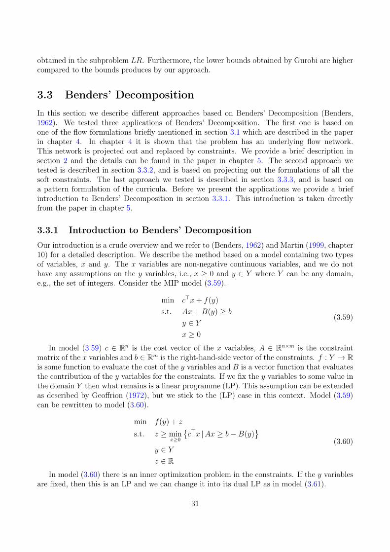
obtained in the subproblem LR. Furthermore, the lower bounds obtained by Gurobi are highercompared to the bounds produces by our approach.

3.3 Benders’ DecompositionIn this section we describe different approaches based on Benders’ Decomposition (Benders,1962). We tested three applications of Benders’ Decomposition. The first one is based onone of the flow formulations briefly mentioned in section 3.1 which are described in the paperin chapter 4. In chapter 4 it is shown that the problem has an underlying flow network.This network is projected out and replaced by constraints. We provide a brief description insection 2 and the details can be found in the paper in chapter 5. The second approach wetested is described in section 3.3.2, and is based on projecting out the formulations of all thesoft constraints. The last approach we tested is described in section 3.3.3, and is based ona pattern formulation of the curricula. Before we present the applications we provide a briefintroduction to Benders’ Decomposition in section 3.3.1. This introduction is taken directlyfrom the paper in chapter 5.

3.3.1 Introduction to Benders’ Decomposition

Our introduction is a crude overview and we refer to (Benders, 1962) and Martin (1999, chapter10) for a detailed description. We describe the method based on a model containing two typesof variables, x and y. The x variables are non-negative continuous variables, and we do nothave any assumptions on the y variables, i.e., x ≥ 0 and y ∈ Y where Y can be any domain,e.g., the set of integers. Consider the MIP model (3.59).

min c>x+ f(y)

s.t. Ax+B(y) ≥ b

y ∈ Yx ≥ 0

(3.59)

In model (3.59) c ∈ Rn is the cost vector of the x variables, A ∈ Rn×m is the constraintmatrix of the x variables and b ∈ Rm is the right-hand-side vector of the constraints. f : Y → Ris some function to evaluate the cost of the y variables and B is a vector function that evaluatesthe contribution of the y variables for the constraints. If we fix the y variables to some value inthe domain Y then what remains is a linear programme (LP). This assumption can be extendedas described by Geoffrion (1972), but we stick to the (LP) case in this context. Model (3.59)can be rewritten to model (3.60).

min f(y) + z

s.t. z ≥ minx≥0

{c>x |Ax ≥ b−B(y)

}y ∈ Yz ∈ R

(3.60)

In model (3.60) there is an inner optimization problem in the constraints. If the y variablesare fixed, then this is an LP and we can change it into its dual LP as in model (3.61).

31

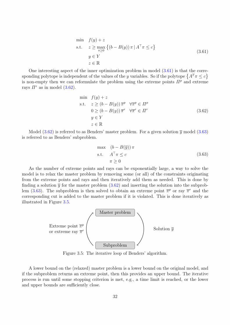
min f(y) + z

s.t. z ≥ maxπ≥0

{(b−B(y))π |A>π ≤ c

}y ∈ Yz ∈ R

(3.61)

One interesting aspect of the inner optimization problem in model (3.61) is that the corre-sponding polytope is independent of the values of the y variables. So if the polytope

{ATπ ≤ c

}is non-empty then we can reformulate the problem using the extreme points Πp and extremerays Πr as in model (3.62).

min f(y) + z

s.t. z ≥ (b−B(y))πp ∀πp ∈ Πp

0 ≥ (b−B(y))πr ∀πr ∈ Πr

y ∈ Yz ∈ R

(3.62)

Model (3.62) is referred to as Benders’ master problem. For a given solution y model (3.63)is referred to as Benders’ subproblem.

max (b−B(y))π

s.t. A>π ≤ c

π ≥ 0

(3.63)

As the number of extreme points and rays can be exponentially large, a way to solve themodel is to relax the master problem by removing some (or all) of the constraints originatingfrom the extreme points and rays and then iteratively add them as needed. This is done byfinding a solution y for the master problem (3.62) and inserting the solution into the subprob-lem (3.63). The subproblem is then solved to obtain an extreme point πp or ray πr and thecorresponding cut is added to the master problem if it is violated. This is done iteratively asillustrated in Figure 3.5.

Master problem

Subproblem

Solution yExtreme point πpor extreme ray πr

Figure 3.5: The iterative loop of Benders’ algorithm.

A lower bound on the (relaxed) master problem is a lower bound on the original model, andif the subproblem returns an extreme point, then this provides an upper bound. The iterativeprocess is run until some stopping criterion is met, e.g., a time limit is reached, or the lowerand upper bounds are sufficiently close.

32

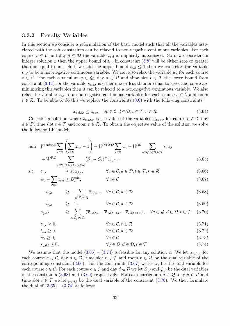
3.3.2 Penalty Variables

In this section we consider a reformulation of the basic model such that all the variables asso-ciated with the soft constraints can be relaxed to non-negative continuous variables. For eachcourse c ∈ C and day d ∈ D the variable tc,d is implicitly maximized. So if we consider aninteger solution x then the upper bound of tc,d in constraint (3.8) will be either zero or greaterthan or equal to one. So if we add the upper bound tc,d ≤ 1 then we can relax the variabletc,d to be a non-negative continuous variable. We can also relax the variable wc for each coursec ∈ C. For each curriculum q ∈ Q, day d ∈ D and time slot t ∈ T the lower bound fromconstraint (3.11) for the variable sq,d,t is either one or less than or equal to zero, and as we areminimizing this variables then it can be relaxed to a non-negative continuous variable. We alsorelax the variable zc,r to a non-negative continuous variables for each course c ∈ C and roomr ∈ R. To be able to do this we replace the constraints (3.6) with the following constraints:

xc,d,t,r ≤ zc,r, ∀c ∈ C, d ∈ D, t ∈ T , r ∈ R (3.64)Consider a solution where xc,d,t,r is the value of the variables xc,d,t,r for course c ∈ C, day

d ∈ D, time slot t ∈ T and room r ∈ R. To obtain the objective value of the solution we solvethe following LP model:

min WRStab∑c∈C

(∑r∈R

zc,r − 1

)+WMWD

∑c∈C

wc +W IL∑

q∈Q,d∈D,t∈T

sq,d,t

+WRC∑

c∈C,d∈D,t∈T ,r∈R

(Sx − Cr)+ xc,d,t,r (3.65)

s.t. zc,r ≥ xc,d,t,r, ∀c ∈ C, d ∈ D, t ∈ T , r ∈ R (3.66)

wc +∑d∈D

tc,d ≥ Dminc , ∀c ∈ C (3.67)

− tc,d ≥ −∑

t∈T ,r∈R

xc,d,t,r, ∀c ∈ C, d ∈ D (3.68)

− tc,d ≥ −1, ∀c ∈ C, d ∈ D (3.69)

sq,d,t ≥∑

c∈Cq ,r∈R

(xc,d,t,r − xc,d,t−1,r − xc,d,t+1,r) , ∀q ∈ Q, d ∈ D, t ∈ T (3.70)

zc,r ≥ 0, ∀c ∈ C, r ∈ R (3.71)tc,d ≥ 0, ∀c ∈ C, d ∈ D (3.72)wc ≥ 0, ∀c ∈ C (3.73)sq,d,t ≥ 0, ∀q ∈ Q, d ∈ D, t ∈ T (3.74)

We assume that the model (3.65) – (3.74) is feasible for any solution x. We let αc,d,t,r foreach course c ∈ C, day d ∈ D, time slot t ∈ T and room r ∈ R be the dual variable of thecorresponding constraint (3.66). For the constraints (3.67) we let πc be the dual variable foreach course c ∈ C. For each course c ∈ C and day d ∈ D we let βc,d and ζc,d be the dual variablesof the constraints (3.68) and (3.69) respectively. For each curriculum q ∈ Q, day d ∈ D andtime slot t ∈ T we let µq,d,t be the dual variable of the constraint (3.70). We then formulatethe dual of (3.65) – (3.74) as follows:

33

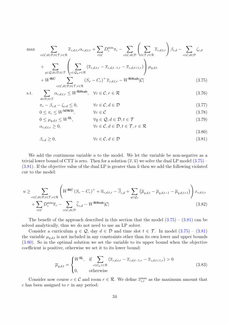
max∑

c∈C,d∈D,t∈T ,r∈R

xc,d,t,rαc,d,t,r +∑c∈C

Dminc πc −

∑c∈C,d∈D

( ∑t∈T ,r∈R

xc,d,t,r

)βc,d −

∑c∈C,d∈D

ζc,d

+∑

q∈Q,d∈D,t∈T

∑c∈Qq ,r∈R

(xc,d,t,r − xc,d,t−1,r − xc,d,t+1,r)

µq,d,t

+WRC∑

c∈C,d∈D,t∈T ,r∈R

(Sx − Cr)+ xc,d,t,r −WRStab|C| (3.75)

s.t.∑

d∈D,t∈T

αc,d,t,r ≤ WRStab, ∀c ∈ C, r ∈ R (3.76)

πc − βc,d − ζc,d ≤ 0, ∀c ∈ C, d ∈ D (3.77)0 ≤ πc ≤ WMWD, ∀c ∈ C (3.78)0 ≤ µq,d,t ≤ W IL, ∀q ∈ Q, d ∈ D, t ∈ T (3.79)αc,d,t,r ≥ 0, ∀c ∈ C, d ∈ D, t ∈ T , r ∈ R

(3.80)βc,d ≥ 0, ∀c ∈ C, d ∈ D (3.81)

We add the continuous variable u to the model. We let the variable be non-negative as atrivial lower bound of CTT is zero. Then for a solution (x, u) we solve the dual LP model (3.75) –(3.81). If the objective value of the dual LP is greater than u then we add the following violatedcut to the model:

u ≥∑

c∈C,d∈D,t∈T ,r∈R

(WRC (Sc − Cr)+ + αc,d,t,r − βc,d +

∑q∈Qc

(µq,d,t − µq,d,t−1 − µq,d,t+1

))xc,d,t,r

+∑c∈C

Dminc πc −

∑c∈C,d∈D

ζc,d −WRStab|C| (3.82)

The benefit of the approach described in this section that the model (3.75) – (3.81) can besolved analytically, thus we do not need to use an LP solver.

Consider a curriculum q ∈ Q, day d ∈ D and time slot t ∈ T . In model (3.75) – (3.81)the variable µq,d,t is not included in any constraints other than its own lower and upper bounds(3.80). So in the optimal solution we set the variable to its upper bound when the objectivecoefficient is positive, otherwise we set it to its lower bound:

µq,d,t =

WIL, if

∑c∈Cq ,r∈R

(xc,d,t,r − xc,d,t−1,r − xc,d,t+1,r) > 0

0, otherwise(3.83)

Consider now course c ∈ C and room r ∈ R. We define xmaxc,r as the maximum amount that

c has been assigned to r in any period:

34

xmaxc,r := max

d∈D,t∈T{xc,d,t,r} (3.84)

In the constraint (3.76) the variables αc,d,t,r for each day d ∈ D and time slot t ∈ T contributeby the same amount and they do not contribute to any other constraints. So we can pick anyvariable αc,d,t,r where xc,d,t,r = xmax

c,r and set it to WRStab and the others to zero. Anotherapproach is to distribute WRStab across all the variables that have the largest coefficient. Wedefine the set Pmax ⊆ D × T as the set of periods where c has been assigned to r by themaximum amount:

Pmax :={d ∈ D, t ∈ T |xc,d,t,r = xmax

c,r

}(3.85)

We then calculate the value αc,d,t,r according to whether or not (d, t) ∈ Pmax:

αc,d,t,r =

WRStab

|Pmax| , if (d, t) ∈ Pmax

0, otherwise(3.86)

The last variables we need to calculate are the ones associated with the calculation of theMWD constraint. Note that the variables π, β and ζ can be calculated separately for eachcourse. Consider course c ∈ C and assume that we know the optimal value πc for the variableπc. Due to constraints (3.77) we have that for the values βc,d and ζc,d for each day d ∈ Dthe sum βc,d + ζc,d is lower bounded by πc. Since all the variables are non-negative and thecoefficients of the variables βc,d and ζc,d for each day d ∈ D are non-positive then it is alwaysdesirable to have the sum at its lower bound:

πc = βc,d + ζc,d (3.87)

As the variables βc,d and ζc,d do not contribute to other constraints then the values βc,d andζc,d can be set such that the variable with the largest (least negative) coefficient is set to πcand the other is set to zero:

βc,d =

πc, if∑

t∈T ,r∈R

xc,d,t,r ≤ 1

0, otherwise(3.88)

ζc,d =

πc, if∑

t∈T ,r∈R

xc,d,t,r > 1

0, otherwise(3.89)

If we insert (3.88) and (3.89) into the objective function then the objective coefficient of πcbecomes the following:

Dminc −

∑d∈D

min

{1,

∑d∈D,t∈T

xc,d,t,r

}(3.90)

So we calculate (3.90) and it is positive then we set πc to its upper bound WMWD and thenwe use (3.88) and (3.89) to calculate the values of the β and ζ variables.

35

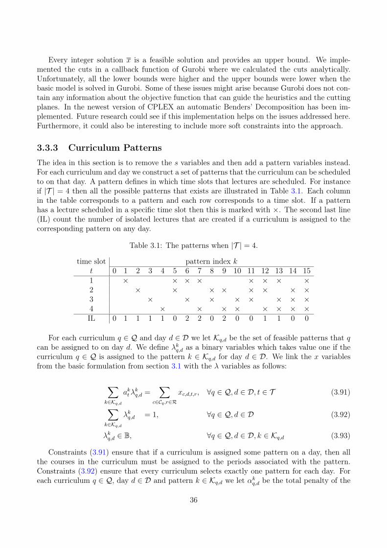
Every integer solution x is a feasible solution and provides an upper bound. We imple-mented the cuts in a callback function of Gurobi where we calculated the cuts analytically.Unfortunately, all the lower bounds were higher and the upper bounds were lower when thebasic model is solved in Gurobi. Some of these issues might arise because Gurobi does not con-tain any information about the objective function that can guide the heuristics and the cuttingplanes. In the newest version of CPLEX an automatic Benders’ Decomposition has been im-plemented. Future research could see if this implementation helps on the issues addressed here.Furthermore, it could also be interesting to include more soft constraints into the approach.

3.3.3 Curriculum Patterns

The idea in this section is to remove the s variables and then add a pattern variables instead.For each curriculum and day we construct a set of patterns that the curriculum can be scheduledto on that day. A pattern defines in which time slots that lectures are scheduled. For instanceif |T | = 4 then all the possible patterns that exists are illustrated in Table 3.1. Each columnin the table corresponds to a pattern and each row corresponds to a time slot. If a patternhas a lecture scheduled in a specific time slot then this is marked with ×. The second last line(IL) count the number of isolated lectures that are created if a curriculum is assigned to thecorresponding pattern on any day.

Table 3.1: The patterns when |T | = 4.

time slot pattern index kt 0 1 2 3 4 5 6 7 8 9 10 11 12 13 14 151 × × × × × × × ×2 × × × × × × × ×3 × × × × × × × ×4 × × × × × × × ×IL 0 1 1 1 1 0 2 2 0 2 0 0 1 1 0 0

For each curriculum q ∈ Q and day d ∈ D we let Kq,d be the set of feasible patterns that qcan be assigned to on day d. We define λkq,d as a binary variables which takes value one if thecurriculum q ∈ Q is assigned to the pattern k ∈ Kq,d for day d ∈ D. We link the x variablesfrom the basic formulation from section 3.1 with the λ variables as follows:

∑k∈Kq,d

akt λkq,d =

∑c∈Cq ,r∈R

xc,d,t,r, ∀q ∈ Q, d ∈ D, t ∈ T (3.91)

∑k∈Kq,d

λkq,d = 1, ∀q ∈ Q, d ∈ D (3.92)

λkq,d ∈ B, ∀q ∈ Q, d ∈ D, k ∈ Kq,d (3.93)

Constraints (3.91) ensure that if a curriculum is assigned some pattern on a day, then allthe courses in the curriculum must be assigned to the periods associated with the pattern.Constraints (3.92) ensure that every curriculum selects exactly one pattern for each day. Foreach curriculum q ∈ Q, day d ∈ D and pattern k ∈ Kq,d we let αkq,d be the total penalty of the

36

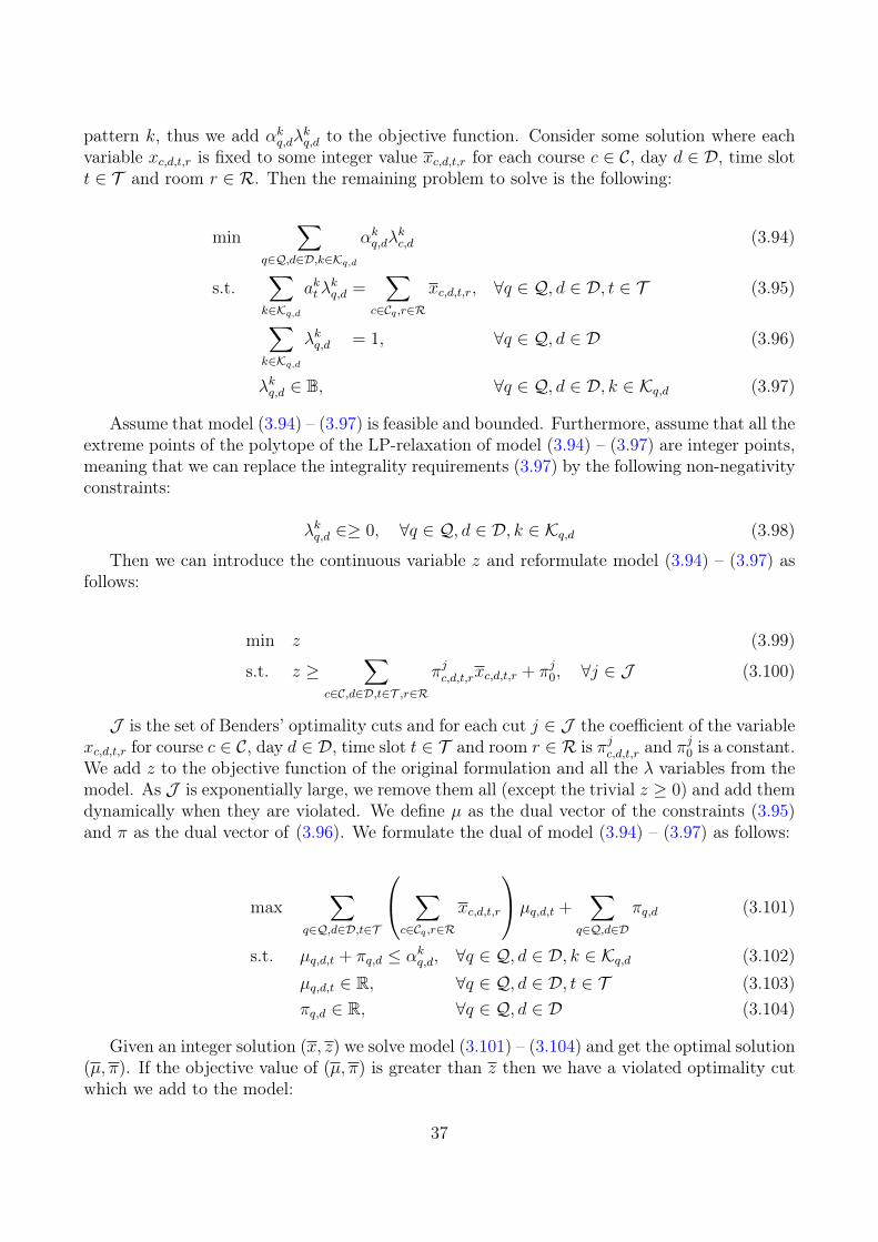
pattern k, thus we add αkq,dλkq,d to the objective function. Consider some solution where eachvariable xc,d,t,r is fixed to some integer value xc,d,t,r for each course c ∈ C, day d ∈ D, time slott ∈ T and room r ∈ R. Then the remaining problem to solve is the following:

min∑

q∈Q,d∈D,k∈Kq,d

αkq,dλkc,d (3.94)

s.t.∑k∈Kq,d

akt λkq,d =

∑c∈Cq ,r∈R

xc,d,t,r, ∀q ∈ Q, d ∈ D, t ∈ T (3.95)

∑k∈Kq,d

λkq,d = 1, ∀q ∈ Q, d ∈ D (3.96)

λkq,d ∈ B, ∀q ∈ Q, d ∈ D, k ∈ Kq,d (3.97)

Assume that model (3.94) – (3.97) is feasible and bounded. Furthermore, assume that all theextreme points of the polytope of the LP-relaxation of model (3.94) – (3.97) are integer points,meaning that we can replace the integrality requirements (3.97) by the following non-negativityconstraints:

λkq,d ∈≥ 0, ∀q ∈ Q, d ∈ D, k ∈ Kq,d (3.98)

Then we can introduce the continuous variable z and reformulate model (3.94) – (3.97) asfollows:

min z (3.99)

s.t. z ≥∑

c∈C,d∈D,t∈T ,r∈R

πjc,d,t,rxc,d,t,r + πj0, ∀j ∈ J (3.100)

J is the set of Benders’ optimality cuts and for each cut j ∈ J the coefficient of the variablexc,d,t,r for course c ∈ C, day d ∈ D, time slot t ∈ T and room r ∈ R is πjc,d,t,r and π

j0 is a constant.

We add z to the objective function of the original formulation and all the λ variables from themodel. As J is exponentially large, we remove them all (except the trivial z ≥ 0) and add themdynamically when they are violated. We define µ as the dual vector of the constraints (3.95)and π as the dual vector of (3.96). We formulate the dual of model (3.94) – (3.97) as follows:

max∑

q∈Q,d∈D,t∈T

∑c∈Cq ,r∈R

xc,d,t,r

µq,d,t +∑

q∈Q,d∈D

πq,d (3.101)

s.t. µq,d,t + πq,d ≤ αkq,d, ∀q ∈ Q, d ∈ D, k ∈ Kq,d (3.102)µq,d,t ∈ R, ∀q ∈ Q, d ∈ D, t ∈ T (3.103)πq,d ∈ R, ∀q ∈ Q, d ∈ D (3.104)

Given an integer solution (x, z) we solve model (3.101) – (3.104) and get the optimal solution(µ, π). If the objective value of (µ, π) is greater than z then we have a violated optimality cutwhich we add to the model:

37

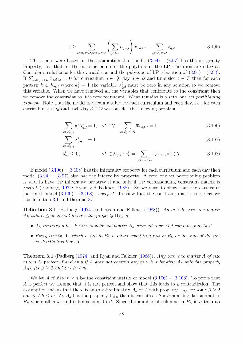
z ≥∑

c∈C,d∈D,t∈T ,r∈R

(∑q∈Qc

µq,d,t

)xc,d,t,r +

∑q∈Q,d∈D

πq,d (3.105)

These cuts were based on the assumption that model (3.94) – (3.97) has the integralityproperty, i.e., that all the extreme points of the polytope of the LP-relaxation are integral.Consider a solution x for the variables x and the polytope of LP relaxation of (3.91) – (3.93).If∑

c∈Cq ,r∈R xc,d,t,r = 0 for curriculum q ∈ Q, day d ∈ D and time slot t ∈ T then for eachpattern k ∈ Kq,d where akt = 1 the variable λkq,d must be zero in any solution so we removethis variable. When we have removed all the variables that contribute to the constraint thenwe remove the constraint as it is now redundant. What remains is a zero–one set partitioningproblem. Note that the model is decomposable for each curriculum and each day, i.e., for eachcurriculum q ∈ Q and each day d ∈ D we consider the following problem:

∑k∈Kq,d

akt λkq,d = 1, ∀t ∈ T :

∑c∈Cq ,r∈R

xc,d,t,r = 1 (3.106)

∑k∈Kq,d

λkq,d = 1 (3.107)

λkq,d ≥ 0, ∀k ∈ Kq,d : akt =∑

c∈Cq ,r∈R

xc,d,t,r, ∀t ∈ T (3.108)

If model (3.106) – (3.108) has the integrality property for each curriculum and each day thenmodel (3.94) – (3.97) also has the integrality property. A zero–one set-partitioning problemis said to have the integrality property if and only if the corresponding constraint matrix isperfect (Padberg, 1974; Ryan and Falkner, 1988). So we need to show that the constraintmatrix of model (3.106) – (3.108) is perfect. To show that the constraint matrix is perfect weuse definition 3.1 and theorem 3.1.

Definition 3.1 (Padberg (1974) and Ryan and Falkner (1988)). An m × h zero–one matrixAh with h ≤ m is said to have the property Πβ,h if:

• Ah contains a h× h non-singular submatrix Bh were all rows and columns sum to β

• Every row in Ah which is not in Bh is either equal to a row in Bh or the sum of the rowis strictly less than β

Theorem 3.1 (Padberg (1974) and Ryan and Falkner (1988)). Any zero–one matrix A of sizem × n is perfect if and only if A does not contain any m × h submatrix Ah with the propertyΠβ,h for β ≥ 2 and 3 ≤ h ≤ m.

We let A of size m× n be the constraint matrix of model (3.106) – (3.108). To prove thatA is perfect we assume that it is not perfect and show that this leads to a contradiction. Theassumption means that there is an m×h submatrix Ah of A with property Πβ,h for some β ≥ 2and 3 ≤ h ≤ m. As Ah has the property Πβ,h then it contains a h× h non-singular submatrixBh where all rows and columns sum to β. Since the number of columns in Bh is h then an

38

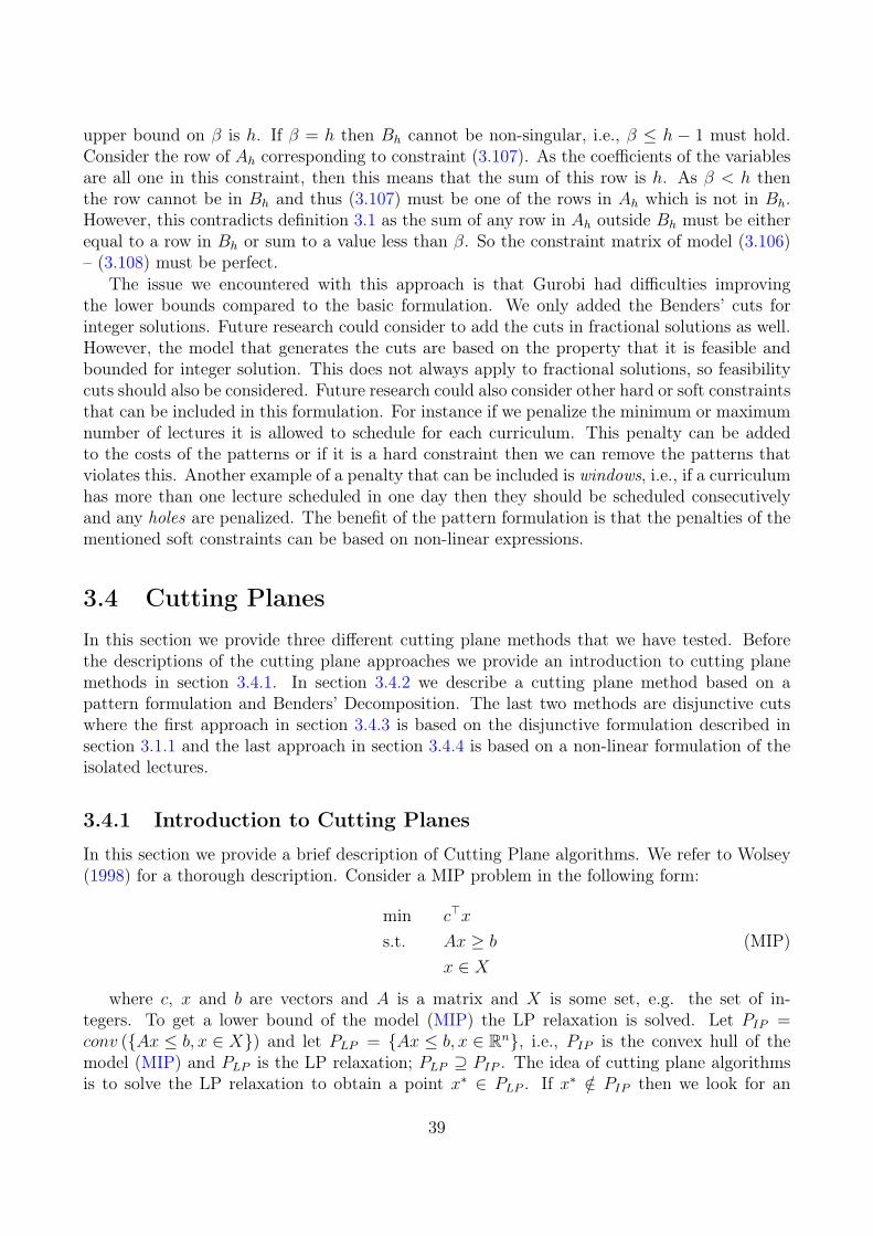
upper bound on β is h. If β = h then Bh cannot be non-singular, i.e., β ≤ h − 1 must hold.Consider the row of Ah corresponding to constraint (3.107). As the coefficients of the variablesare all one in this constraint, then this means that the sum of this row is h. As β < h thenthe row cannot be in Bh and thus (3.107) must be one of the rows in Ah which is not in Bh.However, this contradicts definition 3.1 as the sum of any row in Ah outside Bh must be eitherequal to a row in Bh or sum to a value less than β. So the constraint matrix of model (3.106)– (3.108) must be perfect.

The issue we encountered with this approach is that Gurobi had difficulties improvingthe lower bounds compared to the basic formulation. We only added the Benders’ cuts forinteger solutions. Future research could consider to add the cuts in fractional solutions as well.However, the model that generates the cuts are based on the property that it is feasible andbounded for integer solution. This does not always apply to fractional solutions, so feasibilitycuts should also be considered. Future research could also consider other hard or soft constraintsthat can be included in this formulation. For instance if we penalize the minimum or maximumnumber of lectures it is allowed to schedule for each curriculum. This penalty can be addedto the costs of the patterns or if it is a hard constraint then we can remove the patterns thatviolates this. Another example of a penalty that can be included is windows, i.e., if a curriculumhas more than one lecture scheduled in one day then they should be scheduled consecutivelyand any holes are penalized. The benefit of the pattern formulation is that the penalties of thementioned soft constraints can be based on non-linear expressions.

3.4 Cutting Planes

In this section we provide three different cutting plane methods that we have tested. Beforethe descriptions of the cutting plane approaches we provide an introduction to cutting planemethods in section 3.4.1. In section 3.4.2 we describe a cutting plane method based on apattern formulation and Benders’ Decomposition. The last two methods are disjunctive cutswhere the first approach in section 3.4.3 is based on the disjunctive formulation described insection 3.1.1 and the last approach in section 3.4.4 is based on a non-linear formulation of theisolated lectures.

3.4.1 Introduction to Cutting Planes

In this section we provide a brief description of Cutting Plane algorithms. We refer to Wolsey(1998) for a thorough description. Consider a MIP problem in the following form:

min c>x

s.t. Ax ≥ b

x ∈ X(MIP)

where c, x and b are vectors and A is a matrix and X is some set, e.g. the set of in-tegers. To get a lower bound of the model (MIP) the LP relaxation is solved. Let PIP =conv ({Ax ≤ b, x ∈ X}) and let PLP = {Ax ≤ b, x ∈ Rn}, i.e., PIP is the convex hull of themodel (MIP) and PLP is the LP relaxation; PLP ⊇ PIP . The idea of cutting plane algorithmsis to solve the LP relaxation to obtain a point x∗ ∈ PLP . If x∗ /∈ PIP then we look for an

39

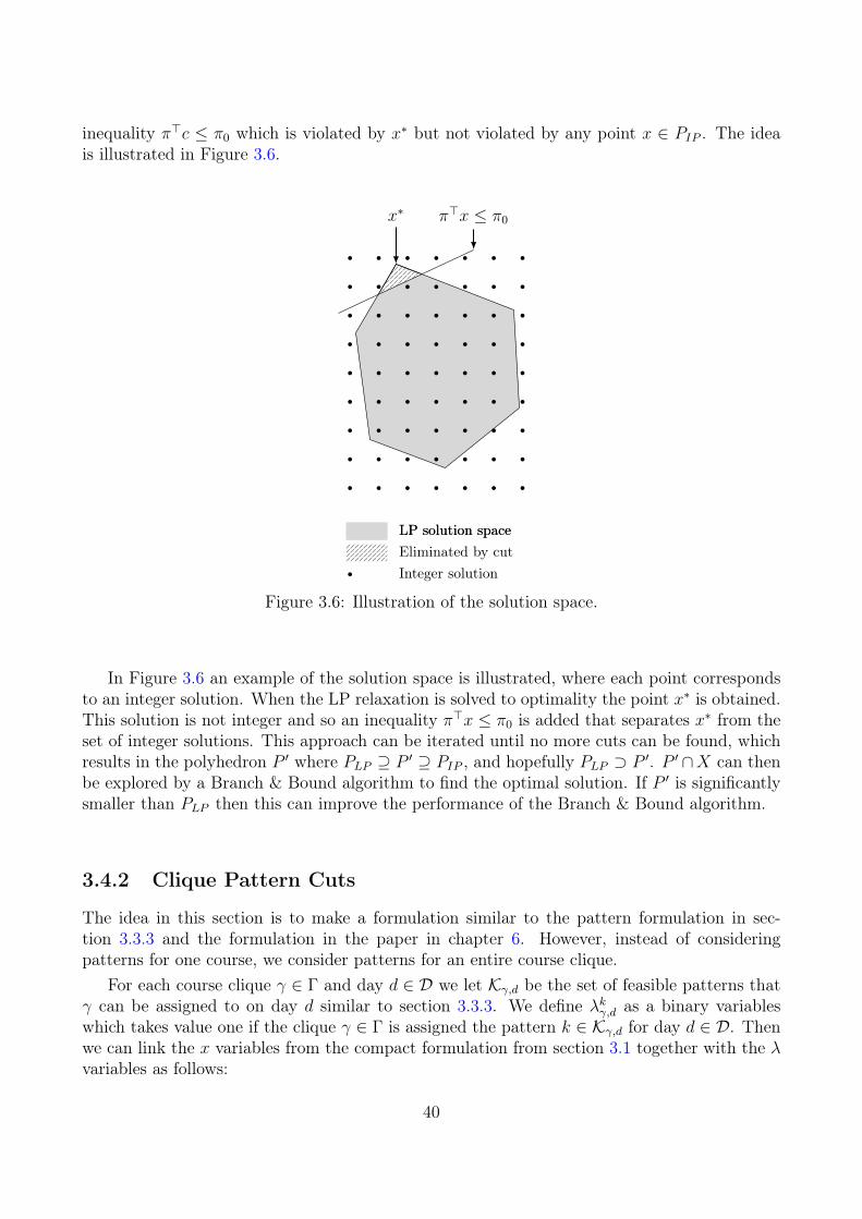
inequality π>c ≤ π0 which is violated by x∗ but not violated by any point x ∈ PIP . The ideais illustrated in Figure 3.6.

x∗ π>x ≤ π0

LP solution spaceLP solution spaceEliminated by cutInteger solution

Figure 3.6: Illustration of the solution space.

In Figure 3.6 an example of the solution space is illustrated, where each point correspondsto an integer solution. When the LP relaxation is solved to optimality the point x∗ is obtained.This solution is not integer and so an inequality π>x ≤ π0 is added that separates x∗ from theset of integer solutions. This approach can be iterated until no more cuts can be found, whichresults in the polyhedron P ′ where PLP ⊇ P ′ ⊇ PIP , and hopefully PLP ⊃ P ′. P ′ ∩X can thenbe explored by a Branch & Bound algorithm to find the optimal solution. If P ′ is significantlysmaller than PLP then this can improve the performance of the Branch & Bound algorithm.

3.4.2 Clique Pattern Cuts

The idea in this section is to make a formulation similar to the pattern formulation in sec-tion 3.3.3 and the formulation in the paper in chapter 6. However, instead of consideringpatterns for one course, we consider patterns for an entire course clique.

For each course clique γ ∈ Γ and day d ∈ D we let Kγ,d be the set of feasible patterns thatγ can be assigned to on day d similar to section 3.3.3. We define λkγ,d as a binary variableswhich takes value one if the clique γ ∈ Γ is assigned the pattern k ∈ Kγ,d for day d ∈ D. Thenwe can link the x variables from the compact formulation from section 3.1 together with the λvariables as follows:

40

∑k∈Kγ,d

akt λkγ,d =

∑c∈Cγ ,r∈R

xc,d,t,r, ∀γ ∈ Γ, d ∈ D, t ∈ T (3.109)

∑k∈Kγ,d

λkγ,d = 1, ∀γ ∈ Γ, d ∈ D (3.110)

λkγ,d ∈ B, ∀γ ∈ Γ, d ∈ D, k ∈ Kγ,d (3.111)

We can prove that the integrality requirements can be replaced by non-negativity constraintby using the same arguments as in section 3.3.3 where we replace the curricula by the coursecliques. The difference between the approach in section 3.3.3 and the approach we considerhere is that we use the the model to generate cuts for fractional solutions. If we are providedwith a fractional solution x then we chec whether the LP-relaxation of model (3.109) – (3.110)is infeasible. If this is the case then we can generate a cut. We do this by introducing newvariables. For each clique γ ∈ Γ, day d ∈ D and time slot t ∈ T we let the variables u+

γ,d,t andu−γ,d,t be the violation of the constraint (3.109). For each clique γ ∈ Γ and day d ∈ D we let thevariables v+

γ,d and v−γ,d be the violation of the constraint (3.110). The objective is to minimizethese variables, i.e., we solve the following model:

min∑

γ∈Γ,d∈D,t∈T

(u+γ,d,t + u−γ,d,t

)+

∑γ∈Γ,d∈D

(v+γ,d + v−γ,d

)(3.112)

s.t.∑k∈Kγ,d

akt λkγ,d + u+

γ,d,t − u−γ,d,t =

∑c∈Cγ ,r∈R

xc,d,t,r, ∀γ ∈ Γ, d ∈ D, t ∈ T (3.113)

∑k∈Kγ,d

λkγ,d + v+γ,d − v

−γ,d = 1, ∀γ ∈ Γ, d ∈ D (3.114)

u+γ,d,t, u

−γ,d,t ≥ 0 ∀γ ∈ Γ, d ∈ D, t ∈ T (3.115)

v+γ,d, v

−γ,d ≥ 0 ∀γ ∈ Γ, d ∈ D (3.116)

λkγ,d ≥ 0, ∀γ ∈ Γ, d ∈ D, k ∈ Kγ,d (3.117)

If the objective value of the optimal solution of model (3.112) – (3.117) is greater than zerothen we can generate a cut to remove the fractional solution x from the solution space of thebasic model. The cut is generated by dualizing model (3.112) – (3.117) as follows:

max∑

γ∈Γ,d∈D,t∈T

∑c∈Cγ ,r∈R

xc,d,t,r

αγ,d,t +∑

γ∈Γ,d∈D

πγ,d (3.118)

s.t. αγ,d,t + πγ,d ≤ 0, ∀γ ∈ Γ, d ∈ D, k ∈ Kγ,d (3.119)− 1 ≤ αγ,d,t ≤ 1, ∀γ ∈ Γ, d ∈ D, t ∈ T (3.120)− 1 ≤ πγ,d ≤ 1, ∀γ ∈ Γ, d ∈ D (3.121)αγ,d,t ∈ R, ∀γ ∈ Γ, d ∈ D, t ∈ T (3.122)πγ,d ∈ R, ∀γ ∈ Γ, d ∈ D (3.123)

41

We solve the model (3.118) – (3.123) and obtain the optimal solution (α, π). If the objectivevalue of this solution is strictly positive then we add the following cut to the basic model:

∑c∈C,d∈D,t∈T

(∑γ∈Γc

αγ,d,t

)xc,d,t +

∑γ∈Γ,d∈D

πγ,d ≤ 0 (3.124)

To improve the strength of the cuts, we also apply a preprocessing phase to remove patternsfrom the set Kγ,d for each clique γ ∈ Γ and day d ∈ D. The preprocessing we apply are takenfrom the paper in chapter 6. All the preprocessing techniques that are discussed in the papercan be applied by extending them to consider course cliques instead of only single courses.Some of the inequalities discussed in the paper can also be applied here, such as the extendedcover inequalities. Furthermore, consider two cliques γ1 ∈ Γ and γ2 ∈ Γ. Let Cγ1,d ⊆ Cγ1 for γ1

be the set of courses where at least one of the time slots on day d ∈ D is available and similarlyfor γ2 we have the set Cγ2,d ⊆ Cγ2 . If Cγ1,d = Cγ2,d then we can remove all the constraintscorresponding to clique γ2 and day d ∈ D as they are redundant.

We implemented the cuts in a callback function of Gurobi where we added any violatedcut to the fractional solution generated by Gurobi in the root node of the Branch & Boundtree. The cuts did not improve the lower bounds compared to Gurobi’s default behaviour. Anyfuture research focusing on this approach should consider if additional valid inequalities can bederived for model (3.112) – (3.117) to strengthen the cuts. It could also be interesting to see ifMIP models for other scheduling problems would benefit from these cuts.

3.4.3 Disjunctive Cuts

In this section we describe an application of adding disjunctive cuts to the basic model. Firstwe provide a brief description of disjunctive cuts, and we refer to Fischetti et al. (2011) for athorough description.

We consider the following MIP model:

min c>x

s.t. Ax ≤ b

x ∈ X(3.125)

Let P be the polyhedron of the LP-relaxation of model (3.125), i.e., P = {Ax ≤ b, x ∈ Rn}where n is the number of variables in the vector x. Assume that we are given a disjunction(PL, PR

)of the model such that every integer point in P is in PR or PL but not in both of them.

We let PL be denoted as{ALx ≤ bL, x ∈ R

}and we let PR be denoted as

{ARx ≤ bR, x ∈ Rn

}.

For any dual vector u ≥ 0 the cut (uAL)>x ≤ ubL is valid for PL and for any dual vectorv ≥ 0 the cut (vAL)>x ≤ vbL is valid for PR. We let ALi be the column in the matrix AL

corresponding to the variable xi and similarly for ARi . We can use these two cuts to generatea valid inequality π>x ≤ π0 for P by calculating π and π0 as follows:

πi = min{uALi , vA

Li

}, i ∈ {1, . . . , n} (3.126)

π0 = max{ubL, vbR

}(3.127)

42

Consider a fractional solution x for the LP relaxation of (3.125). We then formulate thefollowing cut separation problem:

max π>x− π0

s.t. π ≤ uAL

π ≤ vAR

π0 ≥ ubL

π0 ≥ vbR

e>u+ e>v = 1

u, v ≥ 0

π ∈ Rn

π0 ∈ R

(3.128)

The constraint e>u + e>v = 1 is a normalisation constraint that ensures feasibility as themodel can be unbounded. If there exits a solution (π, π0) to model (3.128) where the objectivevalue is positive then x∗ violates the cut π>x ≤ π0 and we add this cut to P .

In the following we describe how we apply the disjunctive cuts for CTT. We apply thecuts for the basic model described in section 3. For the cuts we use the disjunction fromsection 3.1.1. For a fractional solution x consider curriculum q ∈ Q, day d ∈ D and time slott ∈ T where sq,d,t is the value of the variable sq,d,t in the fractional solution. We calculate thesum xq,d,t + xq,d,t−1 + xq,d,t+1, and if the sum is zero or two then we then this is not a branchingcandidate. If the sum if greater than zero and less than two then we calculate the value sDisjq,d,t

according to the disjunctive formulation:

sDisjq,d,t =

{xq,d,t if xq,d,t + xq,d,t−1 + xq,d,t+1 ≤ 1

1− xq,d,t−1 − xq,d,t+1 otherwise(3.129)

If sDisjq,d,t > sq,d,t then this is a candidate for a disjunctive cut. If the sum xq,d,t+xq,d,t−1+xq,d,t+1

is greater than one then we use the disjunction (3.18) for the cut separation problem (3.128).If the sum if less than one then is use the disjunction (3.25). If the sum is one then we pickone of the disjunctions randomly.

In our implementation we used Gurobi and implemented the cutting plane in a callbackfunction. We tested the approach where we added the cuts only in the root node of the Branch& Bound tree. The strategy we used to generate the cuts were to order the candidates by thevalue sDisjq,d,t − sq,d,t from largest to smallest. We then iterated through the list and then addedonly the first cut that was generated. Though cuts were generated, it did not help on theperformance of Gurobi. For future research it could be interesting to examine further if it helpsto add multiple cuts and if the cuts should be added in other nodes in the Branch & Boundtree as well.

3.4.4 Nonlinear Disjunctive Cuts

In this section we consider disjunctive cuts similar to the cuts in section 3.4.3. However, inthis section we consider a disjunction based on a nonlinear formulation of the isolated lectures.

43

Consider a curriculum q ∈ Q, day d ∈ D and time slott ∈ T . Curriculum q has an isolatedlecture in period (d, t) if the variable xq,d,t is one and both xq,d,t−1 and xq,d,t+1 are zero. So wecan replace the constraint (3.11) by the following nonlinear constraint:

sq,d,t = xq,d,t (1− xq,d,t−1) (1− xq,d,t+1) (3.130)

Consider a solution x to the LP relaxation of the basic model. We let sLPq,d,t be the value ofthe variable sq,d,t calculated from the linear formulation (3.11) and sNLPq,d,t be the value calculatedfrom the nonlinear formulation (3.130). Unfortunately the (3.130) is nonlinear and non-convexso we cannot use it in a solver such as Gurobi. However, provided with the solution x to the LPrelaxation, we can calculate the nonlinear terms. In Table 3.2 we have solved the LP relaxationfor all the data instances from ITC2007. For each instance we report the objective value of theLP relaxation in the column LP and in the column NLP we report the objective value of thesame solution if we had used the nonlinear formulation.

Table 3.2: For each instance the objective value of the LP relaxation (LP) is provided as wellas the corresponding objective value for the non-linear formulation

Instance LP NLPcomp01 4.0 51.6comp02 0.0 304.0comp03 0.0 306.4comp04 0.0 210.8comp05 17.0 911.7comp06 6.0 312.3comp07 0.0 325.5comp08 0.0 230.6comp09 0.0 334.1comp10 0.0 253.6comp11 0.0 56.1comp12 3.0 979.0comp13 0.0 262.4comp14 0.0 269.4comp15 0.0 306.4comp16 4.0 319.1comp17 10.0 331.6comp18 0.0 284.6comp19 4.5 271.8comp20 0.0 363.3comp21 0.0 364.8

From Table (3.2) we see that there is a large difference in the objective values, which isalways the case. If we expand the expression (3.130) for the solution x we get the following:

xq,d,t (1− xq,d,t−1) (1− xq,d,t+1) = xq,d,t−xq,d,txq,d,t−1−xq,d,txq,d,t+1 +xq,d,txq,d,t−1xq,d,t+1 (3.131)

44

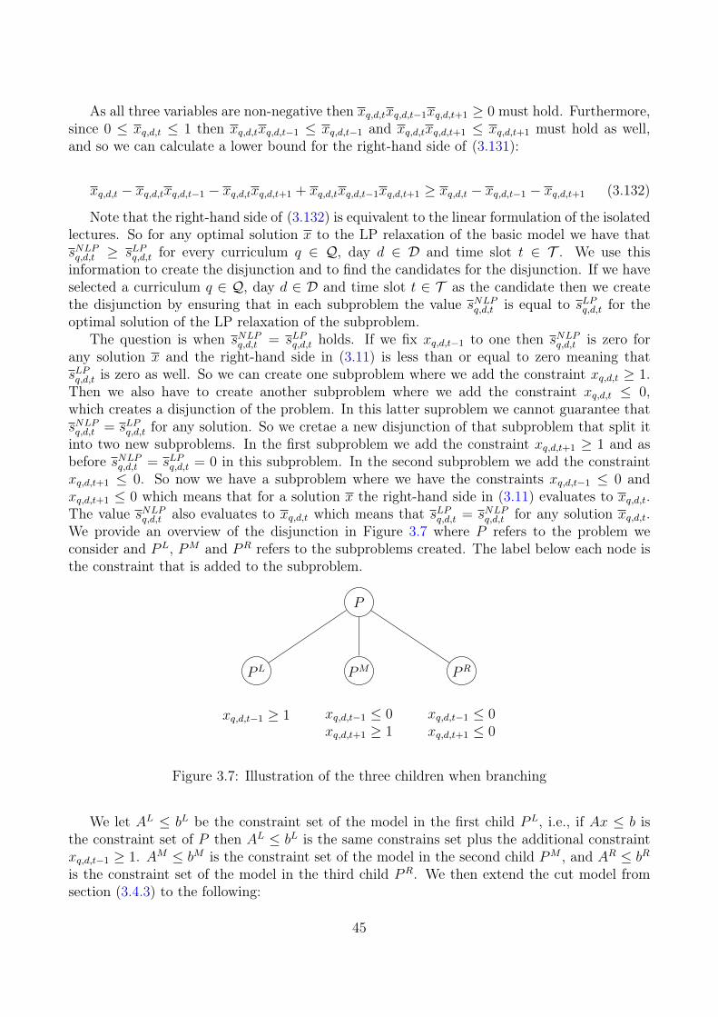
As all three variables are non-negative then xq,d,txq,d,t−1xq,d,t+1 ≥ 0 must hold. Furthermore,since 0 ≤ xq,d,t ≤ 1 then xq,d,txq,d,t−1 ≤ xq,d,t−1 and xq,d,txq,d,t+1 ≤ xq,d,t+1 must hold as well,and so we can calculate a lower bound for the right-hand side of (3.131):

xq,d,t − xq,d,txq,d,t−1 − xq,d,txq,d,t+1 + xq,d,txq,d,t−1xq,d,t+1 ≥ xq,d,t − xq,d,t−1 − xq,d,t+1 (3.132)

Note that the right-hand side of (3.132) is equivalent to the linear formulation of the isolatedlectures. So for any optimal solution x to the LP relaxation of the basic model we have thatsNLPq,d,t ≥ sLPq,d,t for every curriculum q ∈ Q, day d ∈ D and time slot t ∈ T . We use thisinformation to create the disjunction and to find the candidates for the disjunction. If we haveselected a curriculum q ∈ Q, day d ∈ D and time slot t ∈ T as the candidate then we createthe disjunction by ensuring that in each subproblem the value sNLPq,d,t is equal to sLPq,d,t for theoptimal solution of the LP relaxation of the subproblem.

The question is when sNLPq,d,t = sLPq,d,t holds. If we fix xq,d,t−1 to one then sNLPq,d,t is zero forany solution x and the right-hand side in (3.11) is less than or equal to zero meaning thatsLPq,d,t is zero as well. So we can create one subproblem where we add the constraint xq,d,t ≥ 1.Then we also have to create another subproblem where we add the constraint xq,d,t ≤ 0,which creates a disjunction of the problem. In this latter suproblem we cannot guarantee thatsNLPq,d,t = sLPq,d,t for any solution. So we cretae a new disjunction of that subproblem that split itinto two new subproblems. In the first subproblem we add the constraint xq,d,t+1 ≥ 1 and asbefore sNLPq,d,t = sLPq,d,t = 0 in this subproblem. In the second subproblem we add the constraintxq,d,t+1 ≤ 0. So now we have a subproblem where we have the constraints xq,d,t−1 ≤ 0 andxq,d,t+1 ≤ 0 which means that for a solution x the right-hand side in (3.11) evaluates to xq,d,t.The value sNLPq,d,t also evaluates to xq,d,t which means that sLPq,d,t = sNLPq,d,t for any solution xq,d,t.We provide an overview of the disjunction in Figure 3.7 where P refers to the problem weconsider and PL, PM and PR refers to the subproblems created. The label below each node isthe constraint that is added to the subproblem.

P

PL

xq,d,t−1 ≥ 1

PM

xq,d,t−1 ≤ 0xq,d,t+1 ≥ 1

PR

xq,d,t−1 ≤ 0xq,d,t+1 ≤ 0

Figure 3.7: Illustration of the three children when branching

We let AL ≤ bL be the constraint set of the model in the first child PL, i.e., if Ax ≤ b isthe constraint set of P then AL ≤ bL is the same constrains set plus the additional constraintxq,d,t−1 ≥ 1. AM ≤ bM is the constraint set of the model in the second child PM , and AR ≤ bR

is the constraint set of the model in the third child PR. We then extend the cut model fromsection (3.4.3) to the following:

45

max π>x∗ − π0

s.t. π ≤ uAL

π ≤ vAM

π ≤ wAR

π0 ≥ ubL

π0 ≥ vbM

π0 ≥ wbR

e>u+ e>v + e>w = 1

u, v, w ≥ 0

π ∈ Rn

π0 ∈ R

(3.133)

We implemented the cutting plane as a callback function in Gurobi. Whenever we wereprovided with a fractional solution x by Gurobi in the root node of the Branch & Bound tree,we ordered each triple (q, d, t) for curriculum q ∈ Q, day d ∈ D and time slot t ∈ T for thevalue sNLPq,d,t −sLPq,d,t from largest to smallest. We then iteration two the triples and for each triplewe solved the cut separation model (3.133), and if a cut is generated, we add it to the modeland stop. The drawback of this method compared to the disjunctive cuts in section 3.4.3 isthat the cut separation model is larger, which made it more time consuming to solve. It couldbe interesting to see if it help the performance if all the violated cuts and also if the solutiontime of the cut separation process can be improved.

3.5 Dantzig-Wolfe DecompositionIn this section we describe different Dantzig-Wolfe Decomposition that we have considered.Before the description of our implementations, we provide an introduction to Dantzig-WolfeDecomposition in section 3.5.1. This introduction is taken directly from the paper in chapter 7.

Dantzig-Wolfe decompositions have been applied to CTT before, e.g., Cacchiani et al. (2013)mentions different formulations. In one of the decompositions, they decompose one of thesubproblems further when the data instances are large such that there is a subproblem for eachday. In the paper in chapter 7 a decomposition is described that also generates a subproblemfor each day. The difference between Cacchiani et al. (2013) and the paper in chapter 7 is thatthe approach in chapter 7 based on a pattern formulation described in the paper in chapter 6.

In section 3.5.2 and 3.5.3 we describe two other decompositions that we have implementedwhich are also based on the pattern formulation from the paper in chapter 6. The first approachis to decompose the model according to the courses and the second approach divides the courseinto cliques and then decomposes the model according to those cliques.

3.5.1 Introduction to Dantzig-Wolfe Decomposition

Our introduction to the Dantzig-Wolfe Decomposition is specific for MIP models and we refer toMartin (1999, chapter 11) and Desrosiers and Lübbecke (2010) for thorough and more general

46

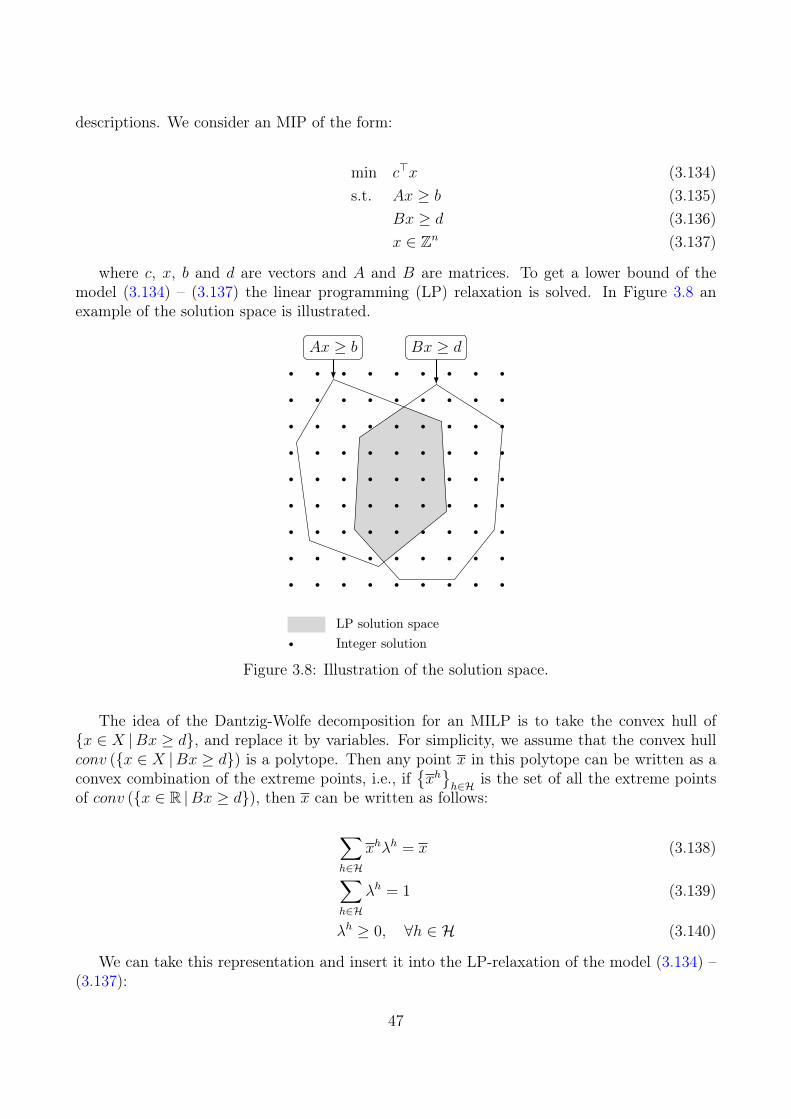
descriptions. We consider an MIP of the form:

min c>x (3.134)s.t. Ax ≥ b (3.135)

Bx ≥ d (3.136)x ∈ Zn (3.137)

where c, x, b and d are vectors and A and B are matrices. To get a lower bound of themodel (3.134) – (3.137) the linear programming (LP) relaxation is solved. In Figure 3.8 anexample of the solution space is illustrated.

Ax ≥ b Bx ≥ d

LP solution spaceInteger solution

Figure 3.8: Illustration of the solution space.

The idea of the Dantzig-Wolfe decomposition for an MILP is to take the convex hull of{x ∈ X |Bx ≥ d}, and replace it by variables. For simplicity, we assume that the convex hullconv ({x ∈ X |Bx ≥ d}) is a polytope. Then any point x in this polytope can be written as aconvex combination of the extreme points, i.e., if

{xh}h∈H is the set of all the extreme points

of conv ({x ∈ R |Bx ≥ d}), then x can be written as follows:

∑h∈H

xhλh = x (3.138)∑h∈H

λh = 1 (3.139)

λh ≥ 0, ∀h ∈ H (3.140)

We can take this representation and insert it into the LP-relaxation of the model (3.134) –(3.137):

47

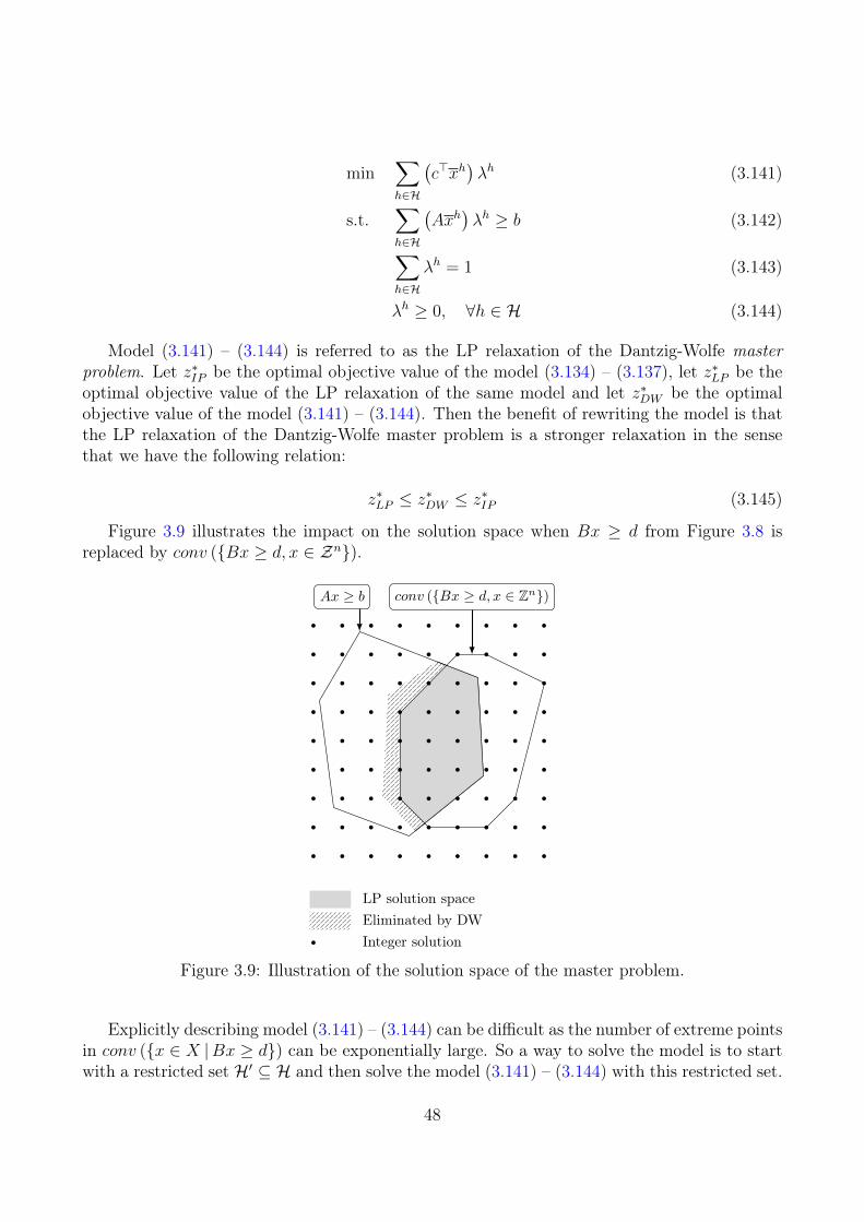
min∑h∈H

(c>xh

)λh (3.141)

s.t.∑h∈H

(Axh

)λh ≥ b (3.142)∑

h∈H

λh = 1 (3.143)

λh ≥ 0, ∀h ∈ H (3.144)

Model (3.141) – (3.144) is referred to as the LP relaxation of the Dantzig-Wolfe masterproblem. Let z∗IP be the optimal objective value of the model (3.134) – (3.137), let z∗LP be theoptimal objective value of the LP relaxation of the same model and let z∗DW be the optimalobjective value of the model (3.141) – (3.144). Then the benefit of rewriting the model is thatthe LP relaxation of the Dantzig-Wolfe master problem is a stronger relaxation in the sensethat we have the following relation:

z∗LP ≤ z∗DW ≤ z∗IP (3.145)

Figure 3.9 illustrates the impact on the solution space when Bx ≥ d from Figure 3.8 isreplaced by conv ({Bx ≥ d, x ∈ Zn}).

Ax ≥ b conv ({Bx ≥ d, x ∈ Zn})

LP solution spaceEliminated by DWInteger solution

Figure 3.9: Illustration of the solution space of the master problem.

Explicitly describing model (3.141) – (3.144) can be difficult as the number of extreme pointsin conv ({x ∈ X |Bx ≥ d}) can be exponentially large. So a way to solve the model is to startwith a restricted set H′ ⊆ H and then solve the model (3.141) – (3.144) with this restricted set.

48

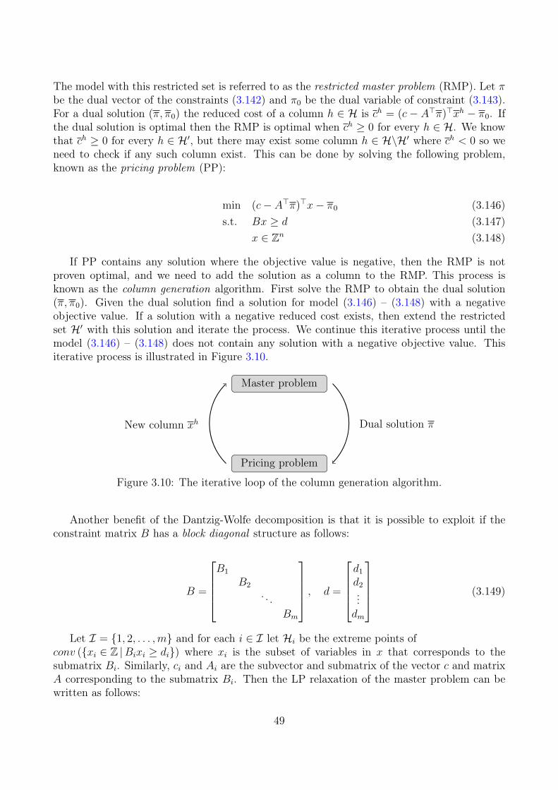
The model with this restricted set is referred to as the restricted master problem (RMP). Let πbe the dual vector of the constraints (3.142) and π0 be the dual variable of constraint (3.143).For a dual solution (π, π0) the reduced cost of a column h ∈ H is ch = (c − A>π)>xh − π0. Ifthe dual solution is optimal then the RMP is optimal when ch ≥ 0 for every h ∈ H. We knowthat ch ≥ 0 for every h ∈ H′, but there may exist some column h ∈ H\H′ where ch < 0 so weneed to check if any such column exist. This can be done by solving the following problem,known as the pricing problem (PP):

min (c− A>π)>x− π0 (3.146)s.t. Bx ≥ d (3.147)

x ∈ Zn (3.148)

If PP contains any solution where the objective value is negative, then the RMP is notproven optimal, and we need to add the solution as a column to the RMP. This process isknown as the column generation algorithm. First solve the RMP to obtain the dual solution(π, π0). Given the dual solution find a solution for model (3.146) – (3.148) with a negativeobjective value. If a solution with a negative reduced cost exists, then extend the restrictedset H′ with this solution and iterate the process. We continue this iterative process until themodel (3.146) – (3.148) does not contain any solution with a negative objective value. Thisiterative process is illustrated in Figure 3.10.

Master problem

Pricing problem

Dual solution πNew column xh

Figure 3.10: The iterative loop of the column generation algorithm.

Another benefit of the Dantzig-Wolfe decomposition is that it is possible to exploit if theconstraint matrix B has a block diagonal structure as follows:

B =

B1

B2

. . .Bm

, d =

d1

d2...dm

(3.149)

Let I = {1, 2, . . . ,m} and for each i ∈ I let Hi be the extreme points ofconv ({xi ∈ Z |Bixi ≥ di}) where xi is the subset of variables in x that corresponds to thesubmatrix Bi. Similarly, ci and Ai are the subvector and submatrix of the vector c and matrixA corresponding to the submatrix Bi. Then the LP relaxation of the master problem can bewritten as follows:

49

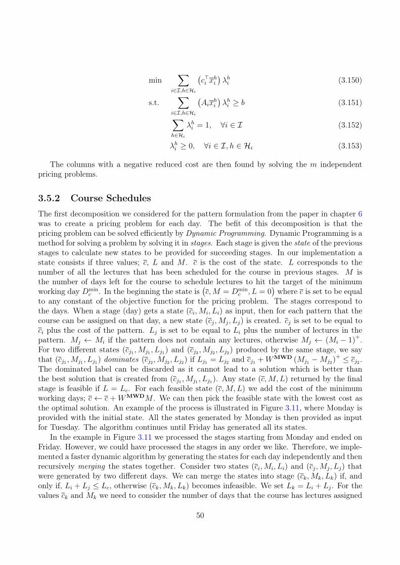
min∑

i∈I,h∈Hi

(c>i x

hi

)λhi (3.150)

s.t.∑

i∈I,h∈Hi

(Aix

hi

)λhi ≥ b (3.151)∑

h∈Hi

λhi = 1, ∀i ∈ I (3.152)

λhi ≥ 0, ∀i ∈ I, h ∈ Hi (3.153)

The columns with a negative reduced cost are then found by solving the m independentpricing problems.

3.5.2 Course Schedules

The first decomposition we considered for the pattern formulation from the paper in chapter 6was to create a pricing problem for each day. The befit of this decomposition is that thepricing problem can be solved efficiently by Dynamic Programming. Dynamic Programming is amethod for solving a problem by solving it in stages. Each stage is given the state of the previousstages to calculate new states to be provided for succeeding stages. In our implementation astate consists if three values; c, L and M . c is the cost of the state. L corresponds to thenumber of all the lectures that has been scheduled for the course in previous stages. M isthe number of days left for the course to schedule lectures to hit the target of the minimumworking day Dmin

c . In the beginning the state is(c,M = Dmin

c , L = 0)where c is set to be equal

to any constant of the objective function for the pricing problem. The stages correspond tothe days. When a stage (day) gets a state (ci,Mi, Li) as input, then for each pattern that thecourse can be assigned on that day, a new state (cj,Mj, Lj) is created. cj is set to be equal toci plus the cost of the pattern. Lj is set to be equal to Li plus the number of lectures in thepattern. Mj ← Mi if the pattern does not contain any lectures, otherwise Mj ← (Mi − 1)+.For two different states (cj1 ,Mj1 , Lj1) and (cj2 ,Mj2 , Lj2) produced by the same stage, we saythat (cj1 ,Mj1 , Lj1) dominates (cj2 ,Mj2 , Lj2) if Lj1 = Lj2 and cj1 +WMWD (Mj1 −Mj2)

+ ≤ cj2 .The dominated label can be discarded as it cannot lead to a solution which is better thanthe best solution that is created from (cj1 ,Mj1 , Lj1). Any state (c,M,L) returned by the finalstage is feasible if L = Lc. For each feasible state (c,M,L) we add the cost of the minimumworking days; c ← c + WMWDM . We can then pick the feasible state with the lowest cost asthe optimal solution. An example of the process is illustrated in Figure 3.11, where Monday isprovided with the initial state. All the states generated by Monday is then provided as inputfor Tuesday. The algorithm continues until Friday has generated all its states.

In the example in Figure 3.11 we processed the stages starting from Monday and ended onFriday. However, we could have processed the stages in any order we like. Therefore, we imple-mented a faster dynamic algorithm by generating the states for each day independently and thenrecursively merging the states together. Consider two states (ci,Mi, Li) and (cj,Mj, Lj) thatwere generated by two different days. We can merge the states into stage (ck,Mk, Lk) if, andonly if, Li + Lj ≤ Lc, otherwise (ck,Mk, Lk) becomes infeasible. We set Lk = Li + Lj. For thevalues ck and Mk we need to consider the number of days that the course has lectures assigned

50

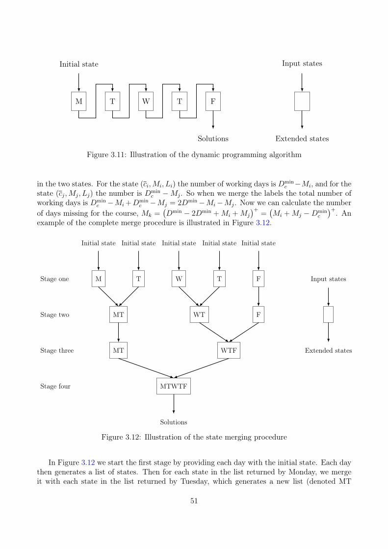
Initial state

M T W T F

Solutions

Input states

Extended states

Figure 3.11: Illustration of the dynamic programming algorithm

in the two states. For the state (ci,Mi, Li) the number of working days is Dminc −Mi, and for the

state (cj,Mj, Lj) the number is Dminc −Mj. So when we merge the labels the total number of

working days is Dminc −Mi +Dmin

c −Mj = 2Dmin−Mi−Mj. Now we can calculate the numberof days missing for the course, Mk =

(Dmin − 2Dmin +Mi +Mj

)+=(Mi +Mj −Dmin

c

)+. Anexample of the complete merge procedure is illustrated in Figure 3.12.

M T W T F

Initial state Initial state Initial state Initial state Initial state

MT WT F

MT WTF

MTWTF

Solutions

Stage one

Stage two

Stage three

Stage four

Input states

Extended states

Figure 3.12: Illustration of the state merging procedure

In Figure 3.12 we start the first stage by providing each day with the initial state. Each daythen generates a list of states. Then for each state in the list returned by Monday, we mergeit with each state in the list returned by Tuesday, which generates a new list (denoted MT

51

in the figure) where the dominated states are discarded. We do the same for Wednesday andThursday (denoted WT in the figure). At this stage we carry over the list of states generatedby Friday (denoted F in the figure), i.e., the states generated by Friday are not merged. In thesecond stage we carry over the list MT to the next stage, and we merge the lists WF and Finto the list WTF. In the third stage we merge the two lists, MT and WTF, which generatesthe list MTWTF. In the last stage we remove all the states where the number of lectures is notLc, and we can then pick the state with the lowest cost as our solution.

3.5.3 Clique Schedules

In this section we describe a decomposition based on the cliques Γ. The formulation is verysimilar to the course decomposition in section 3.5.2, where we also consider the pattern formu-lation from the paper in chapter 6. However, instead of decomposing the model, so we havea pricing problem for each course, we decompose the problem such that each pricing problemcorresponds to a clique of courses. The benefit of this decomposition is that for a clique ofcourses we know that they must be scheduled in different periods. Since each pricing problemcorresponds to a clique, we restrict the columns that are generated by only selecting patternsfor the courses that schedule at most one lecture in each period. The idea is to decompose thecourses into cliques such that each course is contained in exactly one of the cliques. We takethe cliques found by the algorithm described by Bron and Kerbosch (1973) and define a binaryvariable xγ for each clique γ ∈ Γ which is one if the clique is selected for the decomposition,and zero otherwise. For each clique γ ∈ Γ we define the value αγ, which is some measurementof how profitable it is to include γ in the decomposition. We then formulate the decompositionproblem as follows:

max∑γ∈Γ

αγxγ

s.t.∑γ∈Γc

xγ = 1 ∀c ∈ C

x ∈ B

(3.154)

In the model (3.154) there is one constraint for each course, which ensures that the courseis contained in at least one of the selected cliques. For the optimal solution to model (3.154)we decompose the pattern formulation

To ensure that the model (3.154) is feasible we add a clique to Γ for each course c ∈ C, whichcontains only this single course. Let Cq,d,t be defined for curriculum q ∈ Q, day d ∈ D and timeslot t ∈ T as the set of courses that can be scheduled in one of the time slots {t− 1, t, t+ 1}:

Cq,d,t := {c ∈ Cq |Fc,d,t−1 + Fc,d,t + Fc,d,t+1 ≥ 1} , q ∈ Q, d ∈ D, t ∈ T (3.155)

If all the courses in the set Cq,d,t is in a clique γ ∈ Γ, then we can put the formulation ofthe isolated lecture in the corresponding pricing problem. Therefore, we define the profit ofselecting clique γ ∈ Γ to be the number of sets (3.155) where all courses are in the clique:

αγ := ‖{q ∈ Q, d ∈ D, t ∈ T : Cq,d,t ⊆ Cγ}‖ (3.156)

52

For each curriculum q ∈ Q, day d ∈ D and time slot t ∈ T we can also add the set ofcourses Cq,d,t to the set of cliques since Cq,d,t ⊆ Cq. We add these cliques to increase the chancesof the isolated lectures to be included in the pricing problems.

3.5.4 Remarks on the Decompositions

The two formulations from section 3.5.2 and 3.5.3 were not as successful as the decompositionfrom the paper in chapter 6. To get an idea of why this could be the case, we consider theconstraint matrix of the pattern formulation. In Figure 3.13 we illustrate the constraint matrixof the pattern formulation for the data instance comp03 from ITC2007. Each black pixel, exceptthe rectangles, corresponds to a non-zero entry in the matrix. In Figure 3.12a we have orderedthe columns and rows according to courses, in Figure 3.12b we have ordered the columns androws according to the clique decomposition and in Figure 3.12c the columns an rows are orderedby days. The rectangles mark the constraints for the master problem and the block structureof the pricing problem.

It should be noted that for the sake of visualization we added a border around each blockin Figure 3.13. The width of the border is four which is added to the sizes of the matrices.Therefore, the total number of constraints in the pricing problems may appear to be largerthan they are. For instance in Figure 3.12a the total amount of constraints in the pricingproblems appear to be more than half of all the constraints, though, in reality only 5% of theconstraints are in the pricing problems. For the clique decomposition, 43% of the constraintsare in the pricing problems and for the day decomposition, 89% of the constraints are in thepricing problem.

It is mentioned by Martin (1999, chapter 11) that to take full advantage of the Dantzig-WolfeDecomposition procedure the pricing problem must contain a vast majority of the constraints,which is the case for the day decomposition, but not for the other decompositions. Anotherreason that the day decomposition is more successful than the other two is due to the isolatedlectures. In the course decomposition all of the isolated lectures are formulated in the masterproblem, and for the clique decomposition, a few of them are contained in the pricing problems.For the day decomposition, the isolated lectures are contained entirely in the pricing problems.

53

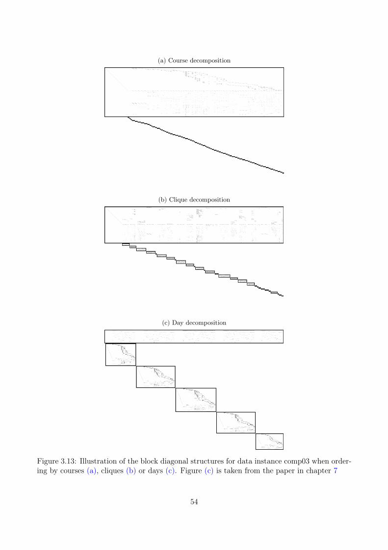
(a) Course decomposition

(b) Clique decomposition

(c) Day decomposition

Figure 3.13: Illustration of the block diagonal structures for data instance comp03 when order-ing by courses (a), cliques (b) or days (c). Figure (c) is taken from the paper in chapter 7

54

References

Asín Aschá, R. and Nieuwenhuis, R. (2014). “Curriculum-based course timetabling with SATand MaxSAT”. In: Annals of Operations Research 218, pp. 71–91.

Bærentsen, R. (2012). “Optimization of room-allocation at the Technical University of Den-mark”. PhD thesis. Technical University of Denmark.

Bagger, N., Kristiansen, S., Sørensen, M., and Stidsen, T. (2015). “Flow Formulation-basedModel for the Curriculum-based Course Timetabling Problem”. In: MISTA 2015 Proceed-ings. Ed. by Z. Hanzálek, G. Kendall, B. McCollum, and P. S̆øucha. Proceedings of the 7thMultidisciplinary International Conference on Scheduling: Theory and Applications (MISTA2015), pp. 825–848.

Benders, J. (1962). “Partitioning procedures for solving mixed-variables programming prob-lems”. English. In: Numerische Mathematik 4.1, pp. 238–252. issn: 0029-599X. doi: 10.1007/BF01386316. url: http://dx.doi.org/10.1007/BF01386316.

Bettinelli, A., Cacchiani, V., Roberti, R., and Toth, P. (2015). “An overview of curriculum-basedcourse timetabling”. In: TOP 23.2, pp. 313–349.

Bonutti, A., De Cesco, F., Di Gaspero, L., and Schaerf, A. (2012). “Benchmarking curriculum-based course timetabling: Formulations, data formats, instances, validation, visualization,and results”. In: Annals of Operations Research 194.1, pp. 59–70.

Bron, C. and Kerbosch, J. (1973). “Algorithm 457: Finding All Cliques of an Undirected Graph”.In: Communications of the ACM 16.9, pp. 575–577. doi: 10.1145/362342.362367. url:http://doi.acm.org/10.1145/362342.362367.

Burke, E. K., Mareček, J., Parkes, A. J., and Rudová, H. (2008). “Penalising Patterns in Timeta-bles: Novel Integer Programming Formulations”. In: Operations Research Proceedings 2007.Springer, pp. 409–414.

Burke, E. K., Mareček, J., Parkes, A. J., and Rudová, H. (2010a). “A supernodal formulation ofvertex colouring with application in course timetabling”. English. In: Annals of OperationsResearch 179.1, pp. 105–130. issn: 0254-5330.

Burke, E. K., Mareček, J., Parkes, A. J., and Rudová, H. (2010b). “Decomposition, reformu-lation, and diving in university course timetabling”. In: Computers & Operations Research37.3, pp. 582–597. doi: 10.1016/j.cor.2009.02.023.

Burke, E. K., Mareček, J., Parkes, A. J., and Rudová, H. (2012). “A branch-and-cut proce-dure for the Udine Course Timetabling problem”. In: Annals of Operations Research 194.1,pp. 71–87.

Cacchiani, V., Caprara, A., Roberti, R., and Toth, P. (2013). “A new lower bound for curriculum-based course timetabling”. In: Computers and Operation Research 40.10, pp. 2466–2477. doi:10.1016/j.cor.2013.02.010.

55

Desrosiers, J. and Lübbecke, M. E. (2010). “A Primer in Column Generation”. In: ColumnGeneration. Ed. by Guy Desaulniers, Jacques Desrosiers, and Marius M. Solomon. SpringerScience+Business Media, Inc. Chap. 1, pp. 1–32. isbn: 978-1-4419-3799-5.

Di Gaspero, L., Schaerf, A., and McCollum, B. (2007). “The Second International TimetablingCompetition (ITC-2007): Curriculum-based Course Timetabling (Track 3) — preliminarypresentation—”. In:Association for the Advancement of Artificial Intelligence (www.aaai.org).

Fischetti, M., Lodi, A., and Tramontani, A. (2011). “On the separation of disjunctive cuts”. In:Mathematical Programming 128.1, pp. 205–230. issn: 1436-4646. doi: 10.1007/s10107-009-0300-y. url: http://dx.doi.org/10.1007/s10107-009-0300-y.

Gamrath, G., Fischer, T., Gally, T., Gleixner, A. M., Hendel, G., Koch, T., Maher, S. J., Mil-tenberger, M., Müller, B., Pfetsch, M. E., Puchert, C., Rehfeldt, D., Schenker, S., Schwarz,R., Serrano, F., Shinano, Y., Vigerske, S., Weninger, D., Winkler, M., Witt, J. T., andWitzig, J. (2016). The SCIP Optimization Suite 3.2. eng. Tech. rep. 15-60. Takustr.7, 14195Berlin: ZIB.

Geoffrion, A. M. (1972). “Generalized benders decomposition”. In: Journal of optimization the-ory and applications 10.4, pp. 237–260.

Gurobi Optimization Inc. (2015). Gurobi Optimizer Reference Manual. url: http://www.gurobi.com.

Gurobi Optimization, Inc. (2016). Gurobi Optimizer Reference Manual. url: http://www.gurobi.com.

Hao, J. K. and Benlic, U. (2011). “Lower bounds for the ITC-2007 curriculum-based coursetimetabling problem”. In: European Journal of Operational Research 212.3, pp. 464–472.

International Business Machines Corp. (2017). IBM ILOG CPLEX Optimization Studio V12.7.0documentation.

Lach, G. and Lübbecke, M. E. (2008). “Optimal University Course Timetables and the Par-tial Transversal Polytope”. In: International Workshop on Experimental and Efficient Algo-rithms. Springer, pp. 235–248.

Lach, G. and Lübbecke, M. E. (2012). “Curriculum based course timetabling: New solutions toUdine benchmark instances”. In: Annals of Operations Research 194.1, pp. 255–272.

Lewis, R., Paechter, B., and McCollum, B. (2007). Post Enrolment based Course Timetabling: ADescription of the Problem Model used for Track Two of the Second International TimetablingCompetition. Cardiff Accounting and Finance Working Papers A2007/3. Cardiff University,Cardiff Business School, Accounting and Finance Section.

Martin, R. K. (1999). Large scale linear and integer optimization: a unified approach. KluwerAcademic Publishers.

McCollum, B., Schaerf, A., Paechter, B., McMullan, P., Lewis, R., Parkes, A. J., Di Gaspero,L., Qu, R., and Burke, E. K. (2010). “Setting the research agenda in automated timetabling:The second international timetabling competition”. In: INFORMS Journal on Computing22.1, pp. 120–130.

Padberg, M.W. (1974). “Perfect zero–one matrices”. In:Mathematical Programming 6.1, pp. 180–196.

Phillips, A. E., Waterer, H., Ehrgott, M., and Ryan, D. M. (2015). “Integer programming meth-ods for large-scale practical classroom assignment problems”. In: Computers & OperationsResearch 53, pp. 42–53. issn: 03050548. doi: 10.1016/j.cor.2014.07.012.

56

Pillay, N. (2016). “A review of hyper-heuristics for educational timetabling”. In: Annals ofOperations Research 239.1, pp. 3–38. issn: 1572-9338. doi: 10.1007/s10479-014-1688-1.url: http://dx.doi.org/10.1007/s10479-014-1688-1.

Ryan, D. M. and Falkner, J. C. (1988). “On the integer properties of scheduling set partitioningmodels”. In: European journal of operational research 35.3, pp. 442–456.

Smith-Miles, K., Baatar, D., Wreford, B., and Lewis, R. (2014). “Towards Objective Measuresof Algorithm Performance Across Instance Space”. In: Comput. Oper. Res. 45, pp. 12–24.issn: 0305-0548. doi: 10.1016/j.cor.2013.11.015. url: http://dx.doi.org/10.1016/j.cor.2013.11.015.

The Scheduling and Timetabling Research Group at the University of Udine, Italy (2015).Curriculum-Based Course TimeTabling. Last retrieved October 2015, http://tabu.diegm.uniud.it/ctt/index.php. url: http://tabu.diegm.uniud.it/ctt/index.php.

Wolsey, L. A. (1998). “Cutting Plane Algorithms”. In: Integer Programming. Ed. by R. Graham,J. Lenstra, and R. Tarjan. John Wiley & Sons, Inc. Chap. 8, pp. 113–137. isbn: 0-471-28366-5.

57

Part II

Exact Methods

59

4 Flow Formulations forCurriculum-based Course Timetabling

Niels-Christian F. Baggera,b · Simon Kristiansenc · Matias Sørensena,b · Thomas R. Stidsena

amORetime research group, Management Science, Department of Management Engineering,Technical University of Denmark, Produktionstorvet, Building 426B, DK-2800 Kgs. Lyngby,Denmark, http://www.moretime.man.dtu.dk/

bMaCom A/S, Vesterbrogade 48, 1., DK-1620 København V, DenmarkcRHA Software Group, Frederikkevej 2B, DK-2900 Hellerup Denmark

Status: Submitted to Annals of Operations Research

Abstract: In this paper we present two mixed-integer programming formulationsfor the Curriculum based Course Timetabling Problem (CTT). We show that theformulations contain underlying network structures by dividing the CTT into twoseparate models and then connect the two models using flow formulation techniques.The first mixed-integer programming formulation is based on an underlying mini-mum cost flow problem, which decreases the number of integer variables significantlyand improves the performance compared to an intuitive mixed-integer programmingformulation. The second formulation is based on a multi-commodity flow problemwhich in general is NP -hard, however, we prove that it suffices to solve the linearprogramming relaxation of the model. The formulations show competitiveness withother approaches based on mixed-integer programming from the literature and im-prove the currently best known lower bound on one data instance in the benchmarkdata set from the second international timetabling competition. Regarding upperbounds, the formulation based on the minimum cost flow problem performs betteron average than other mixed integer programming approaches for the CTT.

Keywords: University Course Timetabling · Integer Programming · MinimumCost Flow · Multi-Commodity Flow

4.1 Description and LiteratureEach semester, universities face the problem of generating high-quality course timetables. Atimetable determines when and where a course should take place. In this work we consider the

61

Curriculum based Course Timetabling (CCT) Problem in which weekly lectures for multiplecourses have to be scheduled and assigned to rooms. A week is divided into days (usually fiveor six) and each day is divided into time slots. We refer to a day and time slot combinationas a period. The problem was introduced in track 3 of the second international timetablingcompetition (ITC2007) as described by Di Gaspero et al. (2007), McCollum et al. (2010) andBonutti et al. (2012).

The basic entities of the problem are the courses to schedule, and the periods and rooms thatare available. Therefore, when formulating a Mixed Integer Program (MIP), it seems naturalto define binary variables with three indices corresponding to a course, period and room wherethe binary variable would then take value one if the course is scheduled in the specified roomat the period. Formulating the MIP of the problem this way is the most commonly used,see Lach and Lübbecke (2008). We show that such a formulation will create an unnecessarilylarge amount of binary variables and instead we formulate two MIPs containing a significantlysmaller number of integer variables. The goal of the formulations is to decrease the number ofinteger variables, and we show that we can define some of the variables as continuous variablesinstead of integer variables.

Besides the courses, periods and rooms the problem also contains lecturers and curricula,hence the name Curriculum-based Course Timetabling. Each course is taught by a lecturer,and a curriculum is a set of courses which may be followed by the same students. The resultingtimetable must fulfil some specific hard constraints:

Availability (A): For each course a subset of the periods (maybe all the periods) are denotedas the available periods. It is not allowed to schedule a lecture in a period that is notavailable for the corresponding course.

Lectures (L): All lectures of all courses must be scheduled, and lectures must be scheduled indifferent periods.

Conflicts (C): If two courses are taught by the same lecturer or the courses are part of thesame curriculum, the courses cannot be taught in the same period.

Room Occupancy (RO): A room can at most be occupied by one course in any period.

Besides the hard constraints, the problem also contains the following soft constraints:

Room Capacity (RC): If a lecture is scheduled in a room where the capacity is smaller thanthe number of students attending the course, then each student above the capacity iscounted as a violation.

Isolated Lectures (IL): It is desired to schedule lectures from the same curriculum in adjacentperiods. Two periods are considered to be adjacent if they belong to the same day andare in consecutive time slots. If a lecture from a curriculum is scheduled in a periodand no lecture from the same curriculum is scheduled in an adjacent period, the lectureis denoted as being isolated. Every time there is an isolated lecture this counts as oneviolation.

Minimum Working Days (MWD): For each course, it is desired to spread the lectures acrossa given number of days. If the number of days that a course is scheduled is below this

62

number, then the violation is the difference between the requested and the actual numberof days that has been scheduled.

Room Stability (RStab): Each course should not be assigned to too many different roomsduring the week. If a course is scheduled in at least two distinct rooms during the week,then the violation is the total number of distinct rooms assigned to the course minus one.

The objective of the CTT is to find a solution which fulfils all the hard constraints andminimizes a weighted sum of the violations of the soft constraints using non-negative weights.

Many researchers have considered the CTT since the ITC2007 competition, and we refer toBettinelli et al. (2015) for an excellent overview. Since we are formulating a MIP model of theproblem, we mainly focus on other MIP based approaches in the literature in the remainder ofthis paper.

Burke et al. (2008) and Burke et al. (2010) introduced a MIP formulation named the mono-lithic formulation, based on the intuition of the three-index binary variables (for each course,period and room a binary variable is defined). The monolithic formulation is an exact model inthe sense that it can be solved by a generic MIP solver to obtain the optimal solution, assumingthat enough computational resources are available for the MIP solver. Unfortunately, manyinstances of the CTT cannot be solved within a reasonable time using a MIP solver for themonolithic formulation. Therefore Burke et al. (2010) propose methods to derive lower andupper bounds based on the monolithic formulation. They obtain one lower bound by ignoringthe soft constraints RC and RStab, which gives the possibility to ignore the assigning of roomsin the formulation. They add a constraint to ensure that no more lectures are scheduled in anyperiod than the number of rooms that are available. They note that the constraint is equivalentto aggregating all the rooms into a single room with a capacity equal to the largest room andthe number of lectures that can be scheduled in this room in a period is equal to the totalnumber of rooms. They use this observation to generate another lower bound by aggregatingthe rooms into multi-rooms. A multi-room is a set of rooms where the capacity is equal to thecapacity of the largest room in the set and the number of lectures that can be scheduled inthe multi-room in a period is equal to the number of rooms in the set. In the tests, they showthat the latter method provides stronger bounds on average. After they obtain a solution fromone of the latter methods a diving heuristic is applied by taking the monolithic formulationand fixing the periods based on the solution from the lower bounding method to obtain a fullsolution. In a more recent paper, Burke et al. (2012) give an exact branch-and-cut algorithmwhich they also base on the monolithic formulation, but some of the objective costs are left outand instead added as cuts during the solution process. Furthermore, some valid inequalities arepresented, which the MIP solver can take advantage of during the search. Their computationalresults show that the cutting plane approach leads to a better performance.

Lach and Lübbecke (2008) and Lach and Lübbecke (2012) propose a method that dividesthe CTT into two stages, where they formulate each stage as a MIP model. In the first stage,they schedule the courses into periods, which only requires a binary variable for each courseand period. They ensure that all the hard constraints are satisfied in the first stage problem.However only the soft constraints MWD, IL and RC can be taken into account. They includethe RC constraints in the first stage by adding a variable for each course, period and distinctroom capacity. In the second stage, they assign the courses to the rooms that the lecturesshould take place in, taking the RStab constraint into consideration. The solution from the

63

first stage is used to fix the courses at the determined periods and the selected room capacitiesin the second stage.

Hao and Benlic (2011) propose a divide-and-conquer approach based on the first stageformulation of Lach and Lübbecke (2012), focusing on finding lower bounds. The methodthey present divides the MIP model into smaller parts by relaxing or removing some of theconstraints such that they can decompose the model into a set of subproblems. They thenobtain lower bounds for each subproblem, and the sum of all these lower bounds is then a lowerbound of the original problem. The approach provides excellent results.

Cacchiani et al. (2013) presented different formulations containing exponentially many vari-ables. The approach that obtained the best computational results consists of two sets of themain binary decision variables. In each of the sets, a binary variable represents a schedulefor an entire week. One of the sets of binary variables takes care of the soft constraints RCand RStab and the other set considers the soft constraints MWD and IL. The sum of thelower bounds of each of the set is a lower bound of the original problem. The method showsimpressive results and obtains good lower bounds.

In the MIP-based methods found in the literature, it seems that decomposing the probleminto smaller parts provides the best results. The downside by many of the methods is thatthey only provide lower bounds or that they come at the cost of sacrificing the guaranteeof optimality, i.e., even if we solve the models to optimality, it does not guarantee that thesolution is globally optimal. Based on these observations, the goal of this paper is to exploit theknowledge that decreasing the number of main decision variables provides better performance.Furthermore, we want to maintain the guarantee of optimality, and therefore we look for exactMIP formulations.

We base our work on the work (Bagger et al., 2015) presented at the biennial Multidis-ciplinary International Scheduling Conference: Theory & Applications (MISTA) 2015 (http://www.schedulingconference.org/). There are some slight differences in this article com-pared to the extended abstract submitted to MISTA. In the abstract, we only discussed oneflow formulation, and in this article we present two flow formulations. Furthermore, there weresome missing details in the proof that we supplied in the appendix (Bagger et al., 2015, Ap-pendix A Proof of Proposition 2). Therefore the proposition and proof have been changed toovercome this and the resulting mathematical model remains the same. Lastly the results havebeen updated with our newest test runs and with more data sets.

We organize the paper as follows: In Section 4.2 an intuitive MIP model is presented, basedon the main binary variables having three indices. We then show how some of the integerrequirements on the variables can be relaxed. In Section 4.3 we present the two formulationsbased on underlying network flow problems; we base the first on a Minimum Cost Flow problemand the second on aMulti-Commodity Flow Problem. We present and discuss the computationalresults in Section 4.4 and lastly some perspectives on the flow formulations are considered inSection 4.5.

Throughout the article, we assume that the reader is familiar with the maximum flowproblem, the minimum cut problem, the minimum cost flow problem, and the multi-commodityflow problem as well as the maximum-flow/minimum-cut theorem. We refer to Kleinberg andTardos (2005) and Ahuja et al. (1993) for details on these problems. Furthermore we definethe following for notation purposes:

64

(x)+ := max {x, 0}

We use the notation Z+ for the set of non-negative integers.

4.2 Three-Index Mixed Integer Programming FormulationIn this section, we present an intuitive MIP formulation of the CTT using three-index bi-nary decision variables. We refer to this formulation throughout the article as the three-indexformulation.

Let C be the set of courses, P be the set of periods and R be the set of rooms. Furthermore,there are days D, curricula Q, lecturers L, the periods Pd ⊆ P that belongs to day d ∈ D, thecourses Cq ⊆ C which are part of curriculum q ∈ Q and the courses Cl ⊆ C which are all beingtaught by lecturer l ∈ L. For each period p ∈ P we define the set Φp. The set Φp containsthe periods that are adjacent to p, i.e. the periods occurring on the same day which is in theperiod directly before or after the time slot of p.

Let Lc be the number of lectures to be scheduled for course c ∈ C, Cr be the capacity ofroom r ∈ R, Sc be the number of students attending course c ∈ C and let Fc,p be one if it isallowed to schedule a lecture from course c ∈ C in period p ∈ P and zero otherwise. Lastly, Mc

is the minimum number of days that it is preferred to schedule lectures for course c ∈ C in.Let xc,p,r be a binary variable deciding whether to schedule a lecture from course c ∈ C in

period p ∈ P and room r ∈ R or not. tc,d is a binary variable taking value one if course c ∈ Chas at least one lecture at day d ∈ D, and zero otherwise. wc is an integer variable denoting thenumber of days below the given minimum that course c ∈ C has lectures. zc,r is a binary variabletaking value one if course c ∈ C is scheduled in room r ∈ R at least once during the week, andzero otherwise. sq,p is a binary variable taking value one if curriculum q ∈ Q has an isolatedlecture in period p ∈ P . Let WRC, W IL, WMWD and WRStab be the non-negative weights ofthe constraints RC, IL, MWD and RStab respectively. The three-index formulation is givenin the following model:

65

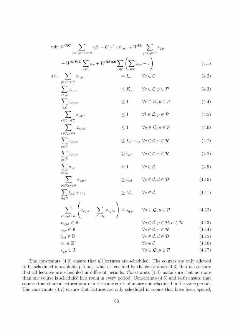
min WRC∑

c∈C,p∈P,r∈R

(Sc − Cr)+ · xc,p,r +W IL∑

q∈Q,p∈P

sq,p

+WMWD∑c∈C

wc +WRStab∑c∈C

(∑r∈R

zc,r − 1

)(4.1)

s.t.∑

p∈P,r∈R

xc,p,r = Lc ∀c ∈ C (4.2)∑r∈R

xc,p,r ≤ Fc,p ∀c ∈ C, p ∈ P (4.3)∑c∈C

xc,p,r ≤ 1 ∀r ∈ R, p ∈ P (4.4)∑c∈Cl,r∈R

xc,p,r ≤ 1 ∀l ∈ L, p ∈ P (4.5)∑c∈Cq ,r∈R

xc,p,r ≤ 1 ∀q ∈ Q, p ∈ P (4.6)

∑p∈P

xc,p,r ≤ Lc · zc,r ∀c ∈ C, r ∈ R (4.7)∑p∈P

xc,p,r ≥ zc,r ∀c ∈ C, r ∈ R (4.8)∑r∈R

zc,r ≥ 1 ∀c ∈ C (4.9)∑p∈Pd,r∈R

xc,p,r ≥ tc,d ∀c ∈ C, d ∈ D (4.10)∑d∈D

tc,d + wc ≥Mc ∀c ∈ C (4.11)

∑c∈Cq ,r∈R

xc,p,r − ∑p′∈Φp

xc,p′,r

≤ sq,p ∀q ∈ Q, p ∈ P (4.12)

xc,p,r ∈ B ∀c ∈ C, p ∈ P , r ∈ R (4.13)zc,r ∈ B ∀c ∈ C, r ∈ R (4.14)tc,d ∈ B ∀c ∈ C, d ∈ D (4.15)wc ∈ Z+ ∀c ∈ C (4.16)sq,p ∈ B ∀q ∈ Q, p ∈ P (4.17)

The constraints (4.2) ensure that all lectures are scheduled. The courses are only allowedto be scheduled in available periods, which is ensured by the constraints (4.3) that also ensurethat all lectures are scheduled in different periods. Constraints (4.4) make sure that no morethan one course is scheduled in a room in every period. Constraints (4.5) and (4.6) ensure thatcourses that share a lecturer or are in the same curriculum are not scheduled in the same period.The constraints (4.7) ensure that lectures are only scheduled in rooms that have been opened,

66

whereby opened we mean a room r ∈ R where zc,r = 1 for course c ∈ C Constraints (4.8) and(4.9) ensure that at least one lecture is scheduled in the open rooms and that at least one roomis put to use by each course. Constraints (4.10) puts an upper bound on the tc,d variable foreach course c ∈ C and day d ∈ D such that it can take a positive value only if at least onelecture for c is scheduled at day d. Constraints (4.11) calculate the violation of the MWDconstraint and the constraints (4.12) calculate for which periods the curricula have isolatedlectures.

The variables tc,d, wc and sq,p can be relaxed to continuous variables, so we replace thevariable domains; (4.15), (4.16) and (4.17) by the following:

0 ≤ tc,d ≤ 1 ∀c ∈ C, d ∈ D (4.18)wc ≥ 0 ∀c ∈ C (4.19)0 ≤ sq,p ≤ 1 ∀q ∈ Q, p ∈ P (4.20)

Burke et al. (2012) note that it is never possible that the minimum workings days constraintis violated by more than Mc − 1 since every course must be scheduled in at least one day.Therefore this can be used as an upper bound for the variable wc which can help the MIPsolver. This bound can be strengthened as all lectures must be scheduled for each course c ∈ Cand therefore the number of days that the course is scheduled in must be at least

⌈Lc|T |

⌉, so we

can add the following bounds:

0 ≤ wc,d ≤Mc −⌈Lc|T |

⌉∀c ∈ C (4.21)

The constraints (4.9) also comes from Burke et al. (2012) where they note that since alllectures must be scheduled then surely every course must occupy at least one room.

If Fc,p = 0 for some course c ∈ C and period p ∈ P then we do not add the variables{xc,p,r}r∈R to the model. Therefore the constraints (4.3) are redundant since every course istaught by exactly one lecturer and constraints (4.5) ensure that each lecturer has at most onelecture scheduled in any period. Furthermore the constraints (4.5) and (4.6) are replaced byclique inequalities. We do this by creating a graph where each node corresponds to a course.An edge is connecting two courses if they are in the same curriculum or taught by the samelecturer. We then enumerate all the maximal cliques by running the Bron-Kerbosch algorithm(Bron and Kerbosch, 1973). Let Γ be the set of cliques and let Cγ be the set of courses in theclique γ ∈ Γ. We replace all the constraints (4.5) and (4.6) by adding the following constraintsfor each clique γ ∈ Γ and period p ∈ P :∑

c∈Cγ ,r∈R

xc,p,r ≤ 1 ∀γ ∈ Γ, p ∈ P (4.22)

4.3 Network Flow FormulationsOur inspiration for the new MIP formulations comes from the two-stage decomposition de-scribed by Lach and Lübbecke (2008) and Lach and Lübbecke (2012). In their work, theysolve the problem by splitting the MIP model into two distinct models and then solve these

67

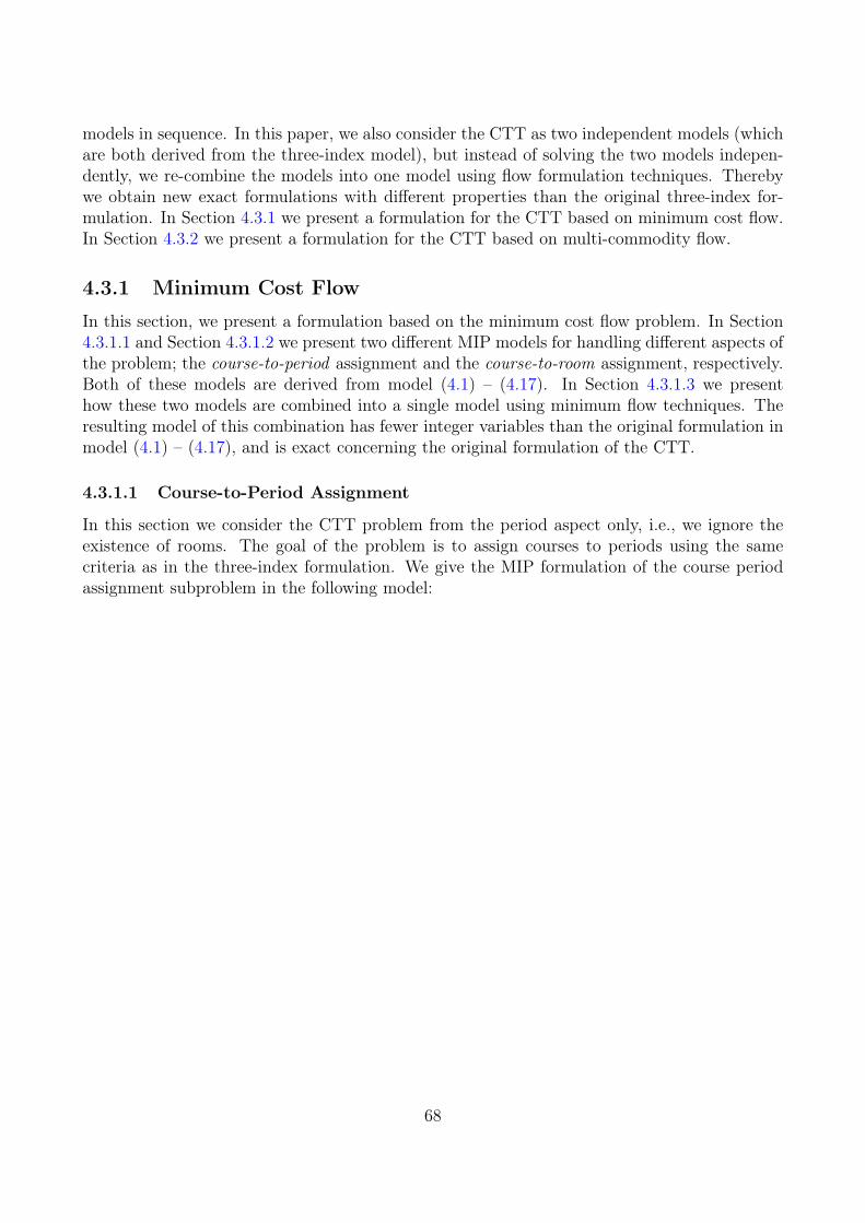
models in sequence. In this paper, we also consider the CTT as two independent models (whichare both derived from the three-index model), but instead of solving the two models indepen-dently, we re-combine the models into one model using flow formulation techniques. Therebywe obtain new exact formulations with different properties than the original three-index for-mulation. In Section 4.3.1 we present a formulation for the CTT based on minimum cost flow.In Section 4.3.2 we present a formulation for the CTT based on multi-commodity flow.

4.3.1 Minimum Cost Flow

In this section, we present a formulation based on the minimum cost flow problem. In Section4.3.1.1 and Section 4.3.1.2 we present two different MIP models for handling different aspects ofthe problem; the course-to-period assignment and the course-to-room assignment, respectively.Both of these models are derived from model (4.1) – (4.17). In Section 4.3.1.3 we presenthow these two models are combined into a single model using minimum flow techniques. Theresulting model of this combination has fewer integer variables than the original formulation inmodel (4.1) – (4.17), and is exact concerning the original formulation of the CTT.

4.3.1.1 Course-to-Period Assignment

In this section we consider the CTT problem from the period aspect only, i.e., we ignore theexistence of rooms. The goal of the problem is to assign courses to periods using the samecriteria as in the three-index formulation. We give the MIP formulation of the course periodassignment subproblem in the following model:

68

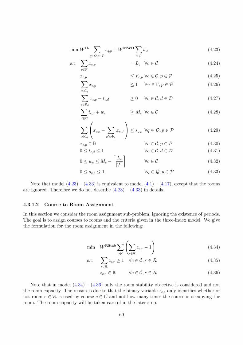
min W IL∑

q∈Q,p∈P

sq,p +WMWD∑c∈C

wc (4.23)

s.t.∑p∈P

xc,p = Lc ∀c ∈ C (4.24)

xc,p ≤ Fc,p ∀c ∈ C, p ∈ P (4.25)∑c∈Cγ

xc,p ≤ 1 ∀γ ∈ Γ, p ∈ P (4.26)

∑p∈Pd

xc,p − tc,d ≥ 0 ∀c ∈ C, d ∈ D (4.27)∑d∈D

tc,d + wc ≥Mc ∀c ∈ C (4.28)

∑c∈Cq

xc,p − ∑p′∈Φp

xc,p′

≤ sq,p ∀q ∈ Q, p ∈ P (4.29)

xc,p ∈ B ∀c ∈ C, p ∈ P (4.30)0 ≤ tc,d ≤ 1 ∀c ∈ C, d ∈ D (4.31)

0 ≤ wc ≤Mc −⌈Lc|T |

⌉∀c ∈ C (4.32)

0 ≤ sq,p ≤ 1 ∀q ∈ Q, p ∈ P (4.33)

Note that model (4.23) – (4.33) is equivalent to model (4.1) – (4.17), except that the roomsare ignored. Therefore we do not describe (4.23) – (4.33) in details.

4.3.1.2 Course-to-Room Assignment

In this section we consider the room assignment sub-problem, ignoring the existence of periods.The goal is to assign courses to rooms and the criteria given in the three-index model. We givethe formulation for the room assignment in the following:

min WRStab∑c∈C

(∑r∈R

zc,r − 1

)(4.34)

s.t.∑r∈R

zc,r ≥ 1 ∀c ∈ C, r ∈ R (4.35)

zc,r ∈ B ∀c ∈ C, r ∈ R (4.36)

Note that in model (4.34) – (4.36) only the room stability objective is considered and notthe room capacity. The reason is due to that the binary variable zc,r only identifies whether ornot room r ∈ R is used by course c ∈ C and not how many times the course is occupying theroom. The room capacity will be taken care of in the later step.

69

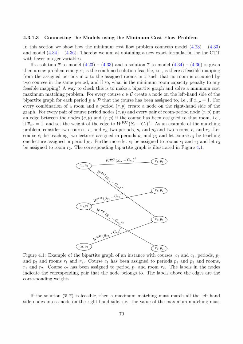
4.3.1.3 Connecting the Models using the Minimum Cost Flow Problem

In this section we show how the minimum cost flow problem connects model (4.23) – (4.33)and model (4.34) – (4.36). Thereby we aim at obtaining a new exact formulation for the CTTwith fewer integer variables.

If a solution x to model (4.23) – (4.33) and a solution z to model (4.34) – (4.36) is giventhen a new problem emerges; is the combined solution feasible, i.e., is there a feasible mappingfrom the assigned periods in x to the assigned rooms in z such that no room is occupied bytwo courses in the same period, and if so, what is the minimum room capacity penalty to anyfeasible mapping? A way to check this is to make a bipartite graph and solve a minimum costmaximum matching problem. For every course c ∈ C create a node on the left-hand side of thebipartite graph for each period p ∈ P that the course has been assigned to, i.e., if xc,p = 1. Forevery combination of a room and a period (r, p) create a node on the right-hand side of thegraph. For every pair of course period nodes (c, p) and every pair of room-period node (r, p) putan edge between the nodes (c, p) and (r, p) if the course has been assigned to that room, i.e.,if zc,r = 1, and set the weight of the edge to WRC (Sc − Cr)+. As an example of the matchingproblem, consider two courses, c1 and c2, two periods, p1 and p2 and two rooms, r1 and r2. Letcourse c1 be teaching two lectures assigned in periods p1 and p2 and let course c2 be teachingone lecture assigned in period p1. Furthermore let c1 be assigned to rooms r1 and r2 and let c2

be assigned to room r2. The corresponding bipartite graph is illustrated in Figure 4.1.

c1, p1

c1, p2

c2, p1

r1, p2

r1, p1

r2, p1

r2, p2

WRC (Sc1 − Cr1)+

W RC

(Sc1 −

Cr2 ) +

WRC (Sc2

− Cr2)+

WRC (Sc1 − Cr1)

+

W RC(Sc1 −

Cr2 ) +

Figure 4.1: Example of the bipartite graph of an instance with courses, c1 and c2, periods, p1

and p2 and rooms r1 and r2. Course c1 has been assigned to periods p1 and p2 and rooms,r1 and r2. Course c2 has been assigned to period p1 and room r2. The labels in the nodesindicate the corresponding pair that the node belongs to. The labels above the edges are thecorresponding weights.

If the solution (x, z) is feasible, then a maximum matching must match all the left-handside nodes into a node on the right-hand side, i.e., the value of the maximum matching must

70

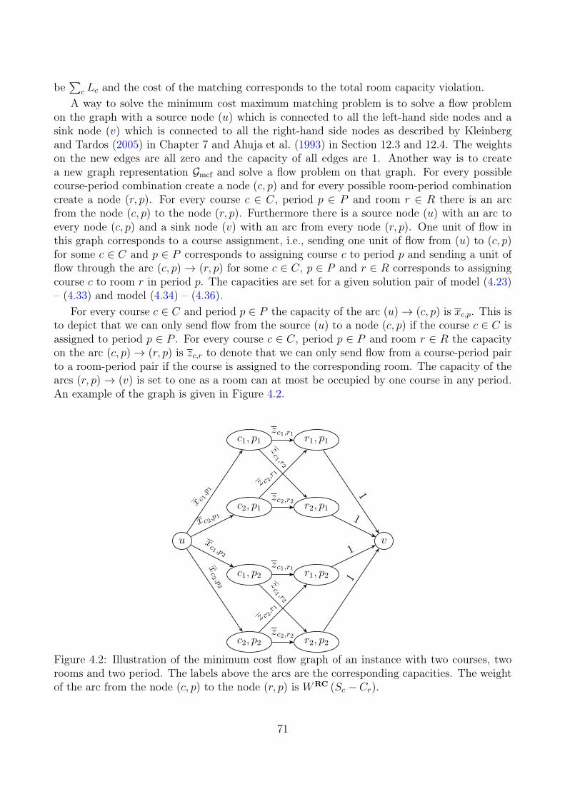
be∑

c Lc and the cost of the matching corresponds to the total room capacity violation.A way to solve the minimum cost maximum matching problem is to solve a flow problem

on the graph with a source node (u) which is connected to all the left-hand side nodes and asink node (v) which is connected to all the right-hand side nodes as described by Kleinbergand Tardos (2005) in Chapter 7 and Ahuja et al. (1993) in Section 12.3 and 12.4. The weightson the new edges are all zero and the capacity of all edges are 1. Another way is to createa new graph representation Gmcf and solve a flow problem on that graph. For every possiblecourse-period combination create a node (c, p) and for every possible room-period combinationcreate a node (r, p). For every course c ∈ C, period p ∈ P and room r ∈ R there is an arcfrom the node (c, p) to the node (r, p). Furthermore there is a source node (u) with an arc toevery node (c, p) and a sink node (v) with an arc from every node (r, p). One unit of flow inthis graph corresponds to a course assignment, i.e., sending one unit of flow from (u) to (c, p)for some c ∈ C and p ∈ P corresponds to assigning course c to period p and sending a unit offlow through the arc (c, p)→ (r, p) for some c ∈ C, p ∈ P and r ∈ R corresponds to assigningcourse c to room r in period p. The capacities are set for a given solution pair of model (4.23)– (4.33) and model (4.34) – (4.36).

For every course c ∈ C and period p ∈ P the capacity of the arc (u)→ (c, p) is xc,p. This isto depict that we can only send flow from the source (u) to a node (c, p) if the course c ∈ C isassigned to period p ∈ P . For every course c ∈ C, period p ∈ P and room r ∈ R the capacityon the arc (c, p)→ (r, p) is zc,r to denote that we can only send flow from a course-period pairto a room-period pair if the course is assigned to the corresponding room. The capacity of thearcs (r, p)→ (v) is set to one as a room can at most be occupied by one course in any period.An example of the graph is given in Figure 4.2.

c1, p1

c2, p1

u

c1, p2

c2, p2

r1, p1

r2, p1

r1, p2

r2, p2

v

x c1,p1

xc2,p1

xc1 ,p2

xc2 ,p

2

zc1,r1

zc1 ,r

2

z c 2,r 1

zc2,r2

zc1,r1

zc1 ,r

2

z c 2,r 1

zc2,r2

1

1

1

1

Figure 4.2: Illustration of the minimum cost flow graph of an instance with two courses, tworooms and two period. The labels above the arcs are the corresponding capacities. The weightof the arc from the node (c, p) to the node (r, p) is WRC (Sc − Cr).

71

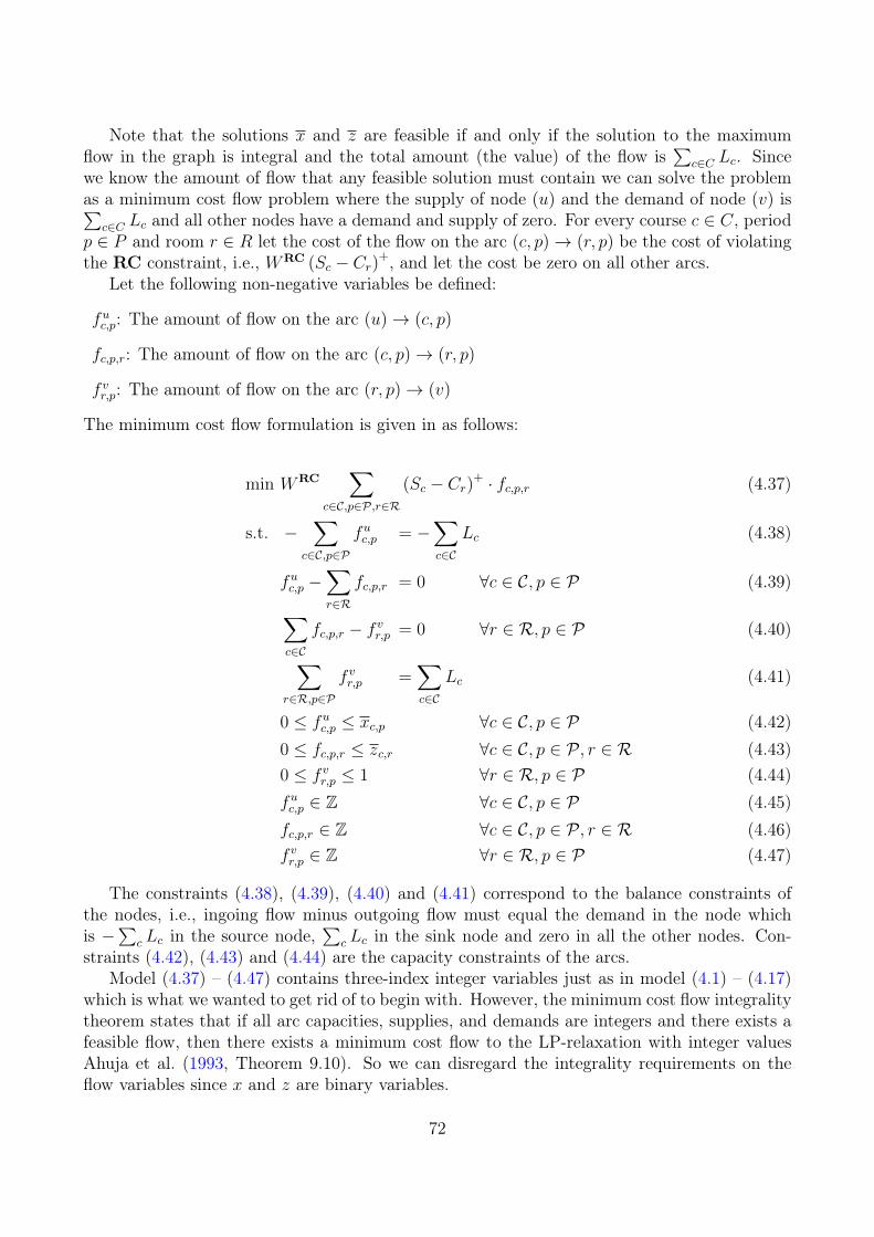
Note that the solutions x and z are feasible if and only if the solution to the maximumflow in the graph is integral and the total amount (the value) of the flow is

∑c∈C Lc. Since

we know the amount of flow that any feasible solution must contain we can solve the problemas a minimum cost flow problem where the supply of node (u) and the demand of node (v) is∑

c∈C Lc and all other nodes have a demand and supply of zero. For every course c ∈ C, periodp ∈ P and room r ∈ R let the cost of the flow on the arc (c, p)→ (r, p) be the cost of violatingthe RC constraint, i.e., WRC (Sc − Cr)+, and let the cost be zero on all other arcs.

Let the following non-negative variables be defined:

fuc,p: The amount of flow on the arc (u)→ (c, p)

fc,p,r: The amount of flow on the arc (c, p)→ (r, p)

f vr,p: The amount of flow on the arc (r, p)→ (v)

The minimum cost flow formulation is given in as follows:

min WRC∑

c∈C,p∈P,r∈R

(Sc − Cr)+ · fc,p,r (4.37)

s.t. −∑

c∈C,p∈P

fuc,p = −∑c∈C

Lc (4.38)

fuc,p −∑r∈R

fc,p,r = 0 ∀c ∈ C, p ∈ P (4.39)∑c∈C

fc,p,r − f vr,p = 0 ∀r ∈ R, p ∈ P (4.40)∑r∈R,p∈P

f vr,p =∑c∈C

Lc (4.41)

0 ≤ fuc,p ≤ xc,p ∀c ∈ C, p ∈ P (4.42)0 ≤ fc,p,r ≤ zc,r ∀c ∈ C, p ∈ P , r ∈ R (4.43)0 ≤ f vr,p ≤ 1 ∀r ∈ R, p ∈ P (4.44)fuc,p ∈ Z ∀c ∈ C, p ∈ P (4.45)fc,p,r ∈ Z ∀c ∈ C, p ∈ P , r ∈ R (4.46)f vr,p ∈ Z ∀r ∈ R, p ∈ P (4.47)

The constraints (4.38), (4.39), (4.40) and (4.41) correspond to the balance constraints ofthe nodes, i.e., ingoing flow minus outgoing flow must equal the demand in the node whichis −

∑c Lc in the source node,

∑c Lc in the sink node and zero in all the other nodes. Con-

straints (4.42), (4.43) and (4.44) are the capacity constraints of the arcs.Model (4.37) – (4.47) contains three-index integer variables just as in model (4.1) – (4.17)

which is what we wanted to get rid of to begin with. However, the minimum cost flow integralitytheorem states that if all arc capacities, supplies, and demands are integers and there exists afeasible flow, then there exists a minimum cost flow to the LP-relaxation with integer valuesAhuja et al. (1993, Theorem 9.10). So we can disregard the integrality requirements on theflow variables since x and z are binary variables.

72

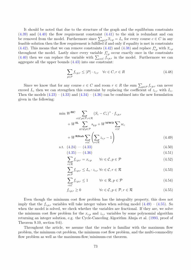
It should be noted that due to the structure of the graph and the equilibrium constraints(4.39) and (4.40) the flow requirement constraint (4.41) to the sink is redundant and canbe removed from the model. Furthermore since

∑p∈P xc,p = Lc for every course c ∈ C in any

feasible solution then the flow requirement is fulfilled if and only if equality is met in constraints(4.42). This means that we can remove constraints (4.42) and (4.38) and replace fuc,p with xc,pthroughout the model. Lastly since every variable f vr,p occur exactly once in the constraints(4.40) then we can replace the variable with

∑c∈C fc,p,r in the model. Furthermore we can

aggregate all the upper bounds (4.43) into one constraint:∑p∈P

fc,p,r ≤ |P | · zc,r ∀c ∈ C, r ∈ R (4.48)

Since we know that for any course c ∈ C and room r ∈ R the sum∑

p∈P fc,p,r can neverexceed Lc then we can strengthen this constraint by replacing the coefficient of zc,r with Lc.Then the models (4.23) – (4.33) and (4.34) – (4.36) can be combined into the new formulationgiven in the following:

min WRC∑

c∈C,p∈P,r∈R

(Sc − Cr)+ · fc,p,r

+W IL∑

q∈Q,p∈P

sq,p +WMWD∑c∈C

wc

+WRStab∑c∈C

(∑r∈R

zc,r − 1

)(4.49)

s.t. (4.24) — (4.33) (4.50)(4.35) — (4.36) (4.51)∑r∈R

fc,p,r = xc,p ∀c ∈ C, p ∈ P (4.52)∑p∈P

fc,p,r ≤ Lc · zc,r ∀c ∈ C, r ∈ R (4.53)∑c∈C

fc,p,r ≤ 1 ∀r ∈ R, p ∈ P (4.54)

fc,p,r ≥ 0 ∀c ∈ C, p ∈ P , r ∈ R (4.55)

Even though the minimum cost flow problem has the integrality property, this does notimply that the fc,p,r variables will take integer values when solving model (4.49) – (4.55). Sowhen the model is solved, we check whether the variables are fractional. If they are, we solvethe minimum cost flow problem for the xc,p and zc,r variables by some polynomial algorithmreturning an integer solution, e.g. the Cycle-Canceling Algorithm Ahuja et al. (1993, proof ofTheorem 9.10, section 9.6).

Throughout the article, we assume that the reader is familiar with the maximum flowproblem, the minimum cut problem, the minimum cost flow problem, and the multi-commodityflow problem as well as the maximum-flow/minimum-cut theorem.

73

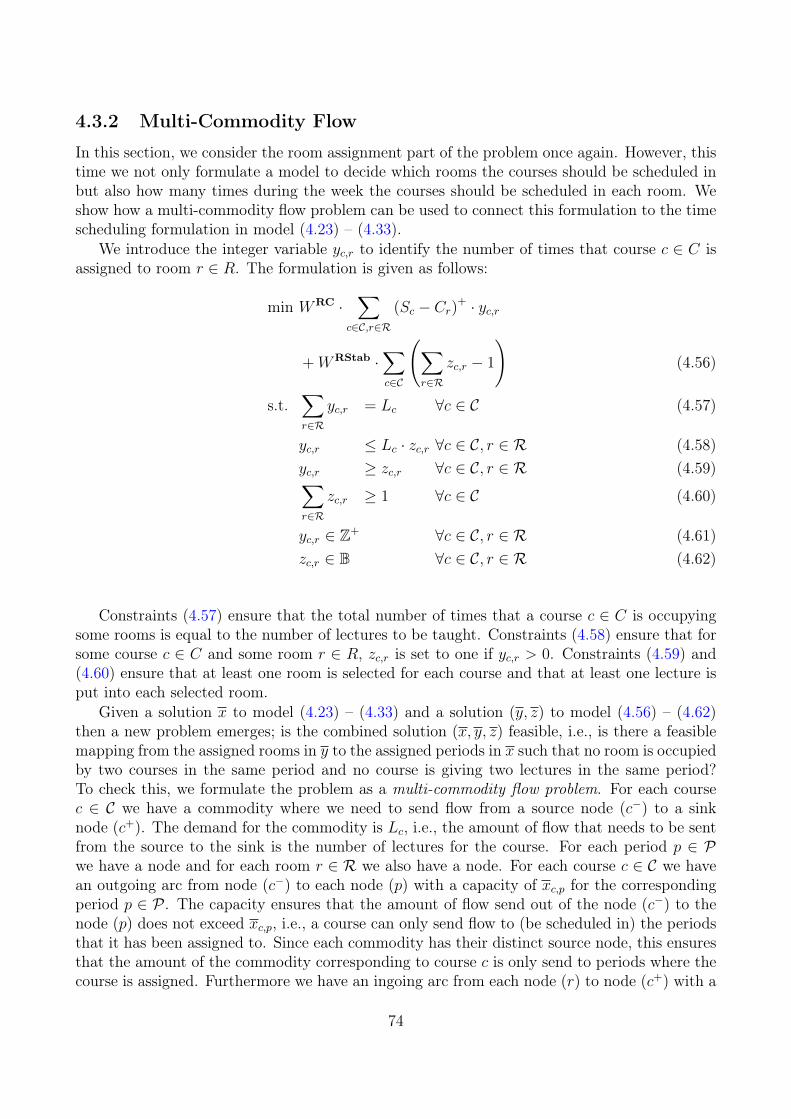
4.3.2 Multi-Commodity Flow

In this section, we consider the room assignment part of the problem once again. However, thistime we not only formulate a model to decide which rooms the courses should be scheduled inbut also how many times during the week the courses should be scheduled in each room. Weshow how a multi-commodity flow problem can be used to connect this formulation to the timescheduling formulation in model (4.23) – (4.33).

We introduce the integer variable yc,r to identify the number of times that course c ∈ C isassigned to room r ∈ R. The formulation is given as follows:

min WRC ·∑

c∈C,r∈R

(Sc − Cr)+ · yc,r

+WRStab ·∑c∈C

(∑r∈R

zc,r − 1

)(4.56)

s.t.∑r∈R

yc,r = Lc ∀c ∈ C (4.57)

yc,r ≤ Lc · zc,r ∀c ∈ C, r ∈ R (4.58)yc,r ≥ zc,r ∀c ∈ C, r ∈ R (4.59)∑r∈R

zc,r ≥ 1 ∀c ∈ C (4.60)

yc,r ∈ Z+ ∀c ∈ C, r ∈ R (4.61)zc,r ∈ B ∀c ∈ C, r ∈ R (4.62)

Constraints (4.57) ensure that the total number of times that a course c ∈ C is occupyingsome rooms is equal to the number of lectures to be taught. Constraints (4.58) ensure that forsome course c ∈ C and some room r ∈ R, zc,r is set to one if yc,r > 0. Constraints (4.59) and(4.60) ensure that at least one room is selected for each course and that at least one lecture isput into each selected room.

Given a solution x to model (4.23) – (4.33) and a solution (y, z) to model (4.56) – (4.62)then a new problem emerges; is the combined solution (x, y, z) feasible, i.e., is there a feasiblemapping from the assigned rooms in y to the assigned periods in x such that no room is occupiedby two courses in the same period and no course is giving two lectures in the same period?To check this, we formulate the problem as a multi-commodity flow problem. For each coursec ∈ C we have a commodity where we need to send flow from a source node (c−) to a sinknode (c+). The demand for the commodity is Lc, i.e., the amount of flow that needs to be sentfrom the source to the sink is the number of lectures for the course. For each period p ∈ Pwe have a node and for each room r ∈ R we also have a node. For each course c ∈ C we havean outgoing arc from node (c−) to each node (p) with a capacity of xc,p for the correspondingperiod p ∈ P . The capacity ensures that the amount of flow send out of the node (c−) to thenode (p) does not exceed xc,p, i.e., a course can only send flow to (be scheduled in) the periodsthat it has been assigned to. Since each commodity has their distinct source node, this ensuresthat the amount of the commodity corresponding to course c is only send to periods where thecourse is assigned. Furthermore we have an ingoing arc from each node (r) to node (c+) with a

74

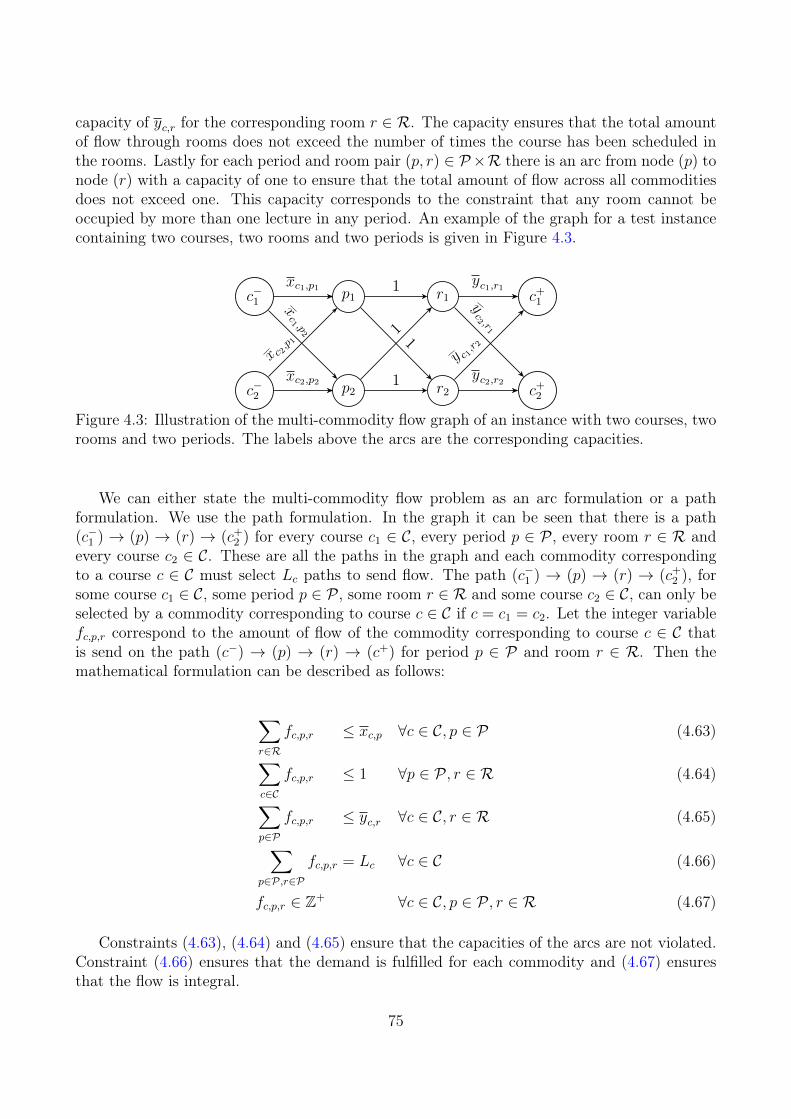
capacity of yc,r for the corresponding room r ∈ R. The capacity ensures that the total amountof flow through rooms does not exceed the number of times the course has been scheduled inthe rooms. Lastly for each period and room pair (p, r) ∈ P×R there is an arc from node (p) tonode (r) with a capacity of one to ensure that the total amount of flow across all commoditiesdoes not exceed one. This capacity corresponds to the constraint that any room cannot beoccupied by more than one lecture in any period. An example of the graph for a test instancecontaining two courses, two rooms and two periods is given in Figure 4.3.

c−1

c−2

p1

p2

r1

r2

c+1

c+2

xc1,p1

x c 2,p 1

xc1 ,p

2

xc2,p2

yc1,r1

y c 1,r 2

yc2 ,r

1

yc2,r2

1

11

1

Figure 4.3: Illustration of the multi-commodity flow graph of an instance with two courses, tworooms and two periods. The labels above the arcs are the corresponding capacities.

We can either state the multi-commodity flow problem as an arc formulation or a pathformulation. We use the path formulation. In the graph it can be seen that there is a path(c−1 ) → (p) → (r) → (c+

2 ) for every course c1 ∈ C, every period p ∈ P , every room r ∈ R andevery course c2 ∈ C. These are all the paths in the graph and each commodity correspondingto a course c ∈ C must select Lc paths to send flow. The path (c−1 ) → (p) → (r) → (c+

2 ), forsome course c1 ∈ C, some period p ∈ P , some room r ∈ R and some course c2 ∈ C, can only beselected by a commodity corresponding to course c ∈ C if c = c1 = c2. Let the integer variablefc,p,r correspond to the amount of flow of the commodity corresponding to course c ∈ C thatis send on the path (c−) → (p) → (r) → (c+) for period p ∈ P and room r ∈ R. Then themathematical formulation can be described as follows:

∑r∈R

fc,p,r ≤ xc,p ∀c ∈ C, p ∈ P (4.63)∑c∈C

fc,p,r ≤ 1 ∀p ∈ P , r ∈ R (4.64)∑p∈P

fc,p,r ≤ yc,r ∀c ∈ C, r ∈ R (4.65)∑p∈P,r∈P

fc,p,r = Lc ∀c ∈ C (4.66)

fc,p,r ∈ Z+ ∀c ∈ C, p ∈ P , r ∈ R (4.67)

Constraints (4.63), (4.64) and (4.65) ensure that the capacities of the arcs are not violated.Constraint (4.66) ensures that the demand is fulfilled for each commodity and (4.67) ensuresthat the flow is integral.

75

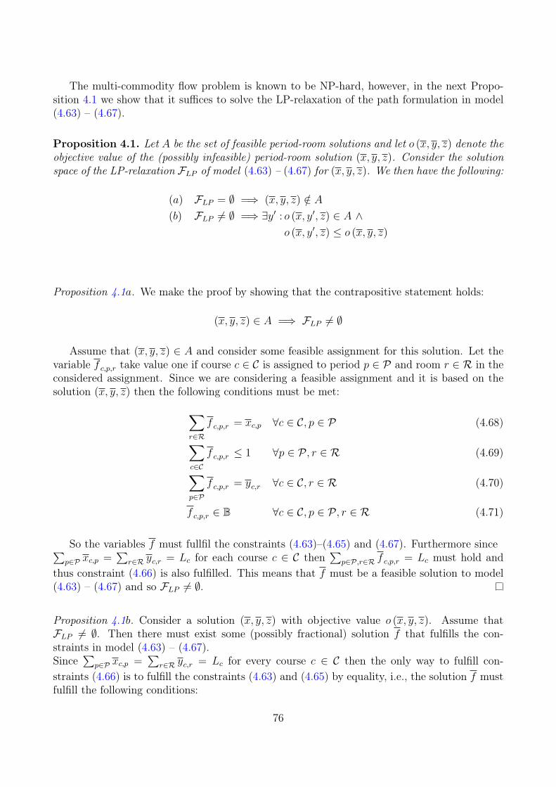
The multi-commodity flow problem is known to be NP-hard, however, in the next Propo-sition 4.1 we show that it suffices to solve the LP-relaxation of the path formulation in model(4.63) – (4.67).

Proposition 4.1. Let A be the set of feasible period-room solutions and let o (x, y, z) denote theobjective value of the (possibly infeasible) period-room solution (x, y, z). Consider the solutionspace of the LP-relaxation FLP of model (4.63) – (4.67) for (x, y, z). We then have the following:

(a) FLP = ∅ =⇒ (x, y, z) /∈ A(b) FLP 6= ∅ =⇒ ∃y′ : o (x, y′, z) ∈ A ∧

o (x, y′, z) ≤ o (x, y, z)

Proposition 4.1a. We make the proof by showing that the contrapositive statement holds:

(x, y, z) ∈ A =⇒ FLP 6= ∅

Assume that (x, y, z) ∈ A and consider some feasible assignment for this solution. Let thevariable f c,p,r take value one if course c ∈ C is assigned to period p ∈ P and room r ∈ R in theconsidered assignment. Since we are considering a feasible assignment and it is based on thesolution (x, y, z) then the following conditions must be met:∑

r∈R

f c,p,r = xc,p ∀c ∈ C, p ∈ P (4.68)∑c∈C

f c,p,r ≤ 1 ∀p ∈ P , r ∈ R (4.69)∑p∈P

f c,p,r = yc,r ∀c ∈ C, r ∈ R (4.70)

f c,p,r ∈ B ∀c ∈ C, p ∈ P , r ∈ R (4.71)

So the variables f must fullfil the constraints (4.63)–(4.65) and (4.67). Furthermore since∑p∈P xc,p =

∑r∈R yc,r = Lc for each course c ∈ C then

∑p∈P,r∈R f c,p,r = Lc must hold and

thus constraint (4.66) is also fulfilled. This means that f must be a feasible solution to model(4.63) – (4.67) and so FLP 6= ∅.

Proposition 4.1b. Consider a solution (x, y, z) with objective value o (x, y, z). Assume thatFLP 6= ∅. Then there must exist some (possibly fractional) solution f that fulfills the con-straints in model (4.63) – (4.67).Since

∑p∈P xc,p =

∑r∈R yc,r = Lc for every course c ∈ C then the only way to fulfill con-

straints (4.66) is to fulfill the constraints (4.63) and (4.65) by equality, i.e., the solution f mustfulfill the following conditions:

76

∑r∈R

f c,p,r = xc,p ∀c ∈ C, p ∈ P (4.72)∑c∈C

f c,p,r ≤ 1 ∀p ∈ P , r ∈ R (4.73)∑p∈P

f c,p,r = yc,r ∀c ∈ C, r ∈ R (4.74)

f c,p,r ≥ 0 ∀c ∈ C, p ∈ C, r ∈ R (4.75)

Now we create a new solution (x, y′, z) where the values x and z are fixed and only thevalues of the y-variables might be changed while ensuring that the objective value does notincrease,i.e., o (x, y′, z) ≤ o (x, y, z). Note that since x and z are kept fixed the difference in the objectivevalue of the two solutions (x, y, z) and (x, y′, z) must be on the RC constraint.

Two cases can occur; either f is integral, or some of the values are fractional. If f is integralthen every value must be either zero or one due to constraint (4.64) and therefore (x, y, z) ∈ Aand we simply set y′ = y.

Consider now the case where f contains fractional values. Since yc,r ≤ Lc · zc,r for eachcourse c ∈ C and each room r ∈ R then we must have that f c,p,r ≤ zc,r for every period p ∈ P .Consider now the minimum cost flow problem as described in Section 4.3.1. A flow f

MCF inthe minimum cost flow graph is created in the following way; for each course c ∈ C, periodp ∈ P and room r ∈ R send flow on the path (u) → (c, p) → (r, p) → (v) equal to f c,p,r. Allthe node balancing constraints must be satisfied as we are considering paths from the sourceto the sink. Furthermore the amount of flow must be

∑c∈C Lc since

∑p∈P xc,p = Lc for each

course c ∈ C and the condition (4.72) holds. Due to the condition (4.72) the capacity of the arc(u)→ (c, p) in the minimum cost flow graph illustrated in Figure 4.2 cannot be violated as thetotal amount of flow on the arc is equal to

∑r∈R f c,p,r and the capacity of the arc is xc,p. For

each course c ∈ C, period p ∈ P and room r ∈ R the capacity of the arc (c, p)→ (r, p), which iszc,r, cannot be violated since the flow send through that arc is equal to f c,p,r and we just arguedthat f c,p,r ≤ zc,r. Lastly since

∑c∈C f c,p,r ≤ 1 then the capacity of the arc (r, p) → (v) in the

graph from Figure 4.2 for room r ∈ R and period p ∈ P cannot be violated. So the flow fMCF

is feasible for the minimum cost flow graph. Recall that the costs on the arcs in the minimumcost flow graph is zero on the arc (u)→ (c, p) for each course c ∈ C and period p ∈ P , zero onthe arc (r, p) → (v) for each room r ∈ R and period p ∈ P and WRC · (Sc − Cr)+ on the arc(c, p)→ (r, p) for each course c ∈ C, period p ∈ P and room r ∈ R. This means that the totalcost of the flow f

MCF is:WRC

∑c∈C,p∈P,r∈R

(Sc − Cr)+ · f c,p,r

Due to the integrality property of the minimum cost flow there must exists a flow f ′ wherethe total amount of flow is the same as for the flow f

MCF, the flow on all the arcs are integersand the cost of the flow f ′ must be less than or equal to the cost of the flow f

MCF:

WRC∑

c∈C,p∈P,r∈R

(Sc − Cr)+ · f ′c,p,r ≤ WRC∑

c∈C,p∈P,r∈R

(Sc − Cr)+ · f c,p,r (4.76)

77

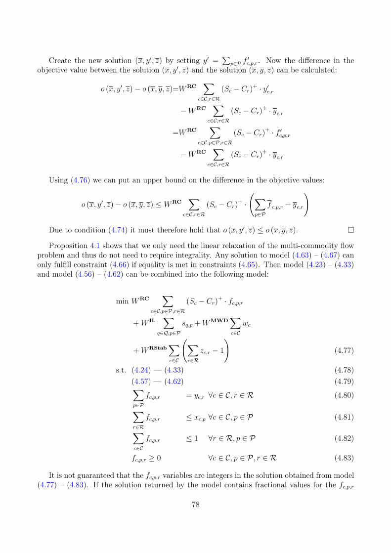
Create the new solution (x, y′, z) by setting y′ =∑

p∈P f′c,p,r. Now the difference in the

objective value between the solution (x, y′, z) and the solution (x, y, z) can be calculated:

o (x, y′, z)− o (x, y, z)=WRC∑

c∈C,r∈R

(Sc − Cr)+ · y′c,r

−WRC∑

c∈C,r∈R

(Sc − Cr)+ · yc,r

=WRC∑

c∈C,p∈P,r∈R

(Sc − Cr)+ · f ′c,p,r

−WRC∑

c∈C,r∈R

(Sc − Cr)+ · yc,r

Using (4.76) we can put an upper bound on the difference in the objective values:

o (x, y′, z)− o (x, y, z) ≤ WRC∑

c∈C,r∈R

(Sc − Cr)+ ·

(∑p∈P

f c,p,r − yc,r

)

Due to condition (4.74) it must therefore hold that o (x, y′, z) ≤ o (x, y, z).

Proposition 4.1 shows that we only need the linear relaxation of the multi-commodity flowproblem and thus do not need to require integrality. Any solution to model (4.63) – (4.67) canonly fulfill constraint (4.66) if equality is met in constraints (4.65). Then model (4.23) – (4.33)and model (4.56) – (4.62) can be combined into the following model:

min WRC∑

c∈C,p∈P,r∈R

(Sc − Cr)+ · fc,p,r

+W IL∑

q∈Q,p∈P

sq,p +WMWD∑c∈C

wc

+WRStab∑c∈C

(∑r∈R

zc,r − 1

)(4.77)

s.t. (4.24) — (4.33) (4.78)(4.57) — (4.62) (4.79)∑p∈P

fc,p,r = yc,r ∀c ∈ C, r ∈ R (4.80)∑r∈R

fc,p,r ≤ xc,p ∀c ∈ C, p ∈ P (4.81)∑c∈C

fc,p,r ≤ 1 ∀r ∈ R, p ∈ P (4.82)

fc,p,r ≥ 0 ∀c ∈ C, p ∈ P , r ∈ R (4.83)

It is not guaranteed that the fc,p,r variables are integers in the solution obtained from model(4.77) – (4.83). If the solution returned by the model contains fractional values for the fc,p,r

78

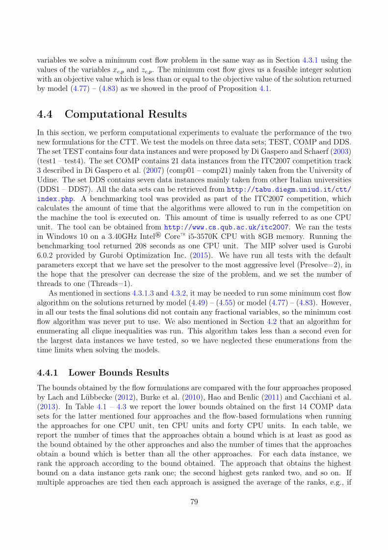
variables we solve a minimum cost flow problem in the same way as in Section 4.3.1 using thevalues of the variables xc,p and zc,p. The minimum cost flow gives us a feasible integer solutionwith an objective value which is less than or equal to the objective value of the solution returnedby model (4.77) – (4.83) as we showed in the proof of Proposition 4.1.

4.4 Computational ResultsIn this section, we perform computational experiments to evaluate the performance of the twonew formulations for the CTT. We test the models on three data sets; TEST, COMP and DDS.The set TEST contains four data instances and were proposed by Di Gaspero and Schaerf (2003)(test1 – test4). The set COMP contains 21 data instances from the ITC2007 competition track3 described in Di Gaspero et al. (2007) (comp01 – comp21) mainly taken from the University ofUdine. The set DDS contains seven data instances mainly taken from other Italian universities(DDS1 – DDS7). All the data sets can be retrieved from http://tabu.diegm.uniud.it/ctt/index.php. A benchmarking tool was provided as part of the ITC2007 competition, whichcalculates the amount of time that the algorithms were allowed to run in the competition onthe machine the tool is executed on. This amount of time is usually referred to as one CPUunit. The tool can be obtained from http://www.cs.qub.ac.uk/itc2007. We ran the testsin Windows 10 on a 3.40GHz Intel® Core™ i5-3570K CPU with 8GB memory. Running thebenchmarking tool returned 208 seconds as one CPU unit. The MIP solver used is Gurobi6.0.2 provided by Gurobi Optimization Inc. (2015). We have run all tests with the defaultparameters except that we have set the presolver to the most aggressive level (Presolve=2), inthe hope that the presolver can decrease the size of the problem, and we set the number ofthreads to one (Threads=1).

As mentioned in sections 4.3.1.3 and 4.3.2, it may be needed to run some minimum cost flowalgorithm on the solutions returned by model (4.49) – (4.55) or model (4.77) – (4.83). However,in all our tests the final solutions did not contain any fractional variables, so the minimum costflow algorithm was never put to use. We also mentioned in Section 4.2 that an algorithm forenumerating all clique inequalities was run. This algorithm takes less than a second even forthe largest data instances we have tested, so we have neglected these enumerations from thetime limits when solving the models.

4.4.1 Lower Bounds Results

The bounds obtained by the flow formulations are compared with the four approaches proposedby Lach and Lübbecke (2012), Burke et al. (2010), Hao and Benlic (2011) and Cacchiani et al.(2013). In Table 4.1 – 4.3 we report the lower bounds obtained on the first 14 COMP datasets for the latter mentioned four approaches and the flow-based formulations when runningthe approaches for one CPU unit, ten CPU units and forty CPU units. In each table, wereport the number of times that the approaches obtain a bound which is at least as good asthe bound obtained by the other approaches and also the number of times that the approachesobtain a bound which is better than all the other approaches. For each data instance, werank the approach according to the bound obtained. The approach that obtains the highestbound on a data instance gets rank one; the second highest gets ranked two, and so on. Ifmultiple approaches are tied then each approach is assigned the average of the ranks, e.g., if

79

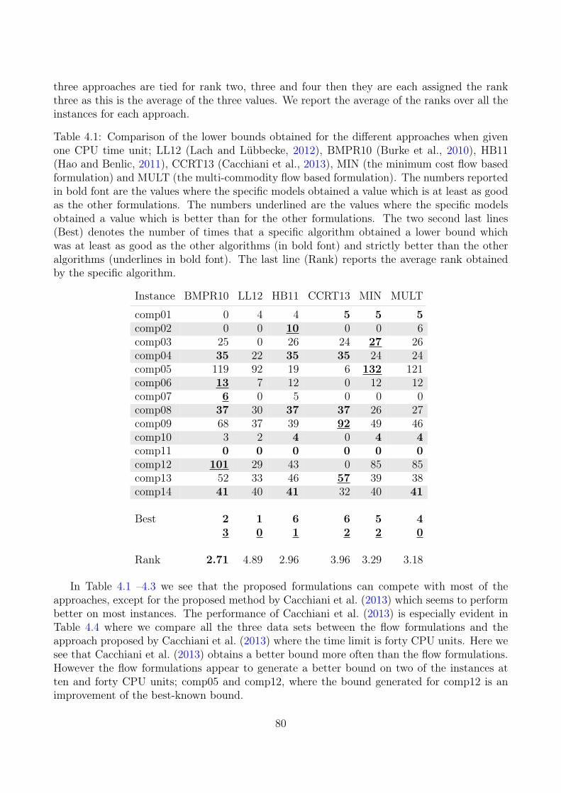
three approaches are tied for rank two, three and four then they are each assigned the rankthree as this is the average of the three values. We report the average of the ranks over all theinstances for each approach.

Table 4.1: Comparison of the lower bounds obtained for the different approaches when givenone CPU time unit; LL12 (Lach and Lübbecke, 2012), BMPR10 (Burke et al., 2010), HB11(Hao and Benlic, 2011), CCRT13 (Cacchiani et al., 2013), MIN (the minimum cost flow basedformulation) and MULT (the multi-commodity flow based formulation). The numbers reportedin bold font are the values where the specific models obtained a value which is at least as goodas the other formulations. The numbers underlined are the values where the specific modelsobtained a value which is better than for the other formulations. The two second last lines(Best) denotes the number of times that a specific algorithm obtained a lower bound whichwas at least as good as the other algorithms (in bold font) and strictly better than the otheralgorithms (underlines in bold font). The last line (Rank) reports the average rank obtainedby the specific algorithm.

Instance BMPR10 LL12 HB11 CCRT13 MIN MULT

comp01 0 4 4 5 5 5comp02 0 0 10 0 0 6comp03 25 0 26 24 27 26comp04 35 22 35 35 24 24comp05 119 92 19 6 132 121comp06 13 7 12 0 12 12comp07 6 0 5 0 0 0comp08 37 30 37 37 26 27comp09 68 37 39 92 49 46comp10 3 2 4 0 4 4comp11 0 0 0 0 0 0comp12 101 29 43 0 85 85comp13 52 33 46 57 39 38comp14 41 40 41 32 40 41

Best 2 1 6 6 5 43 0 1 2 2 0

Rank 2.71 4.89 2.96 3.96 3.29 3.18

In Table 4.1 –4.3 we see that the proposed formulations can compete with most of theapproaches, except for the proposed method by Cacchiani et al. (2013) which seems to performbetter on most instances. The performance of Cacchiani et al. (2013) is especially evident inTable 4.4 where we compare all the three data sets between the flow formulations and theapproach proposed by Cacchiani et al. (2013) where the time limit is forty CPU units. Here wesee that Cacchiani et al. (2013) obtains a better bound more often than the flow formulations.However the flow formulations appear to generate a better bound on two of the instances atten and forty CPU units; comp05 and comp12, where the bound generated for comp12 is animprovement of the best-known bound.

80

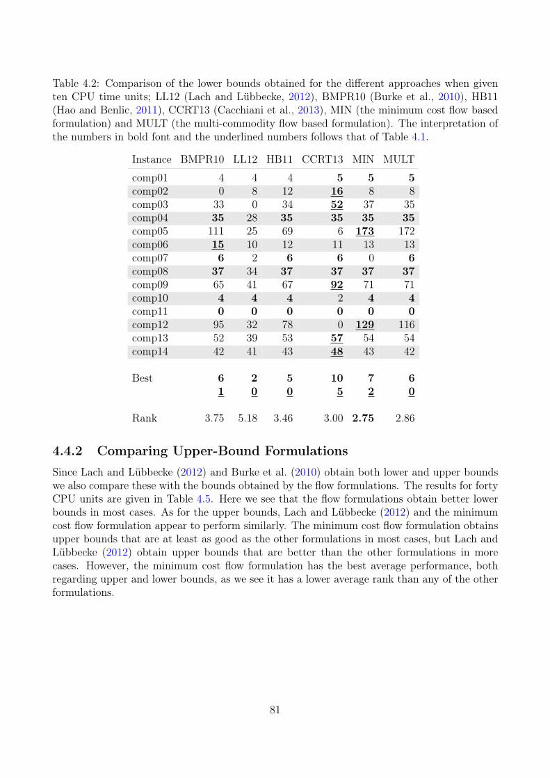
Table 4.2: Comparison of the lower bounds obtained for the different approaches when giventen CPU time units; LL12 (Lach and Lübbecke, 2012), BMPR10 (Burke et al., 2010), HB11(Hao and Benlic, 2011), CCRT13 (Cacchiani et al., 2013), MIN (the minimum cost flow basedformulation) and MULT (the multi-commodity flow based formulation). The interpretation ofthe numbers in bold font and the underlined numbers follows that of Table 4.1.

Instance BMPR10 LL12 HB11 CCRT13 MIN MULT

comp01 4 4 4 5 5 5comp02 0 8 12 16 8 8comp03 33 0 34 52 37 35comp04 35 28 35 35 35 35comp05 111 25 69 6 173 172comp06 15 10 12 11 13 13comp07 6 2 6 6 0 6comp08 37 34 37 37 37 37comp09 65 41 67 92 71 71comp10 4 4 4 2 4 4comp11 0 0 0 0 0 0comp12 95 32 78 0 129 116comp13 52 39 53 57 54 54comp14 42 41 43 48 43 42

Best 6 2 5 10 7 61 0 0 5 2 0

Rank 3.75 5.18 3.46 3.00 2.75 2.86

4.4.2 Comparing Upper-Bound Formulations

Since Lach and Lübbecke (2012) and Burke et al. (2010) obtain both lower and upper boundswe also compare these with the bounds obtained by the flow formulations. The results for fortyCPU units are given in Table 4.5. Here we see that the flow formulations obtain better lowerbounds in most cases. As for the upper bounds, Lach and Lübbecke (2012) and the minimumcost flow formulation appear to perform similarly. The minimum cost flow formulation obtainsupper bounds that are at least as good as the other formulations in most cases, but Lach andLübbecke (2012) obtain upper bounds that are better than the other formulations in morecases. However, the minimum cost flow formulation has the best average performance, bothregarding upper and lower bounds, as we see it has a lower average rank than any of the otherformulations.

81

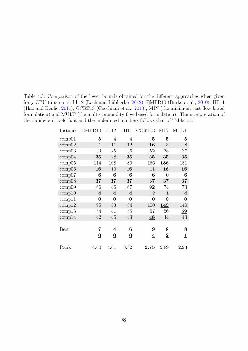
Table 4.3: Comparison of the lower bounds obtained for the different approaches when givenforty CPU time units; LL12 (Lach and Lübbecke, 2012), BMPR10 (Burke et al., 2010), HB11(Hao and Benlic, 2011), CCRT13 (Cacchiani et al., 2013), MIN (the minimum cost flow basedformulation) and MULT (the multi-commodity flow based formulation). The interpretation ofthe numbers in bold font and the underlined numbers follows that of Table 4.1.

Instance BMPR10 LL12 HB11 CCRT13 MIN MULT

comp01 5 4 4 5 5 5comp02 1 11 12 16 8 8comp03 33 25 36 52 38 37comp04 35 28 35 35 35 35comp05 114 108 80 166 186 181comp06 16 10 16 11 16 16comp07 6 6 6 6 0 6comp08 37 37 37 37 37 37comp09 66 46 67 92 74 73comp10 4 4 4 2 4 4comp11 0 0 0 0 0 0comp12 95 53 84 100 142 140comp13 54 41 55 57 56 59comp14 42 46 43 48 44 43

Best 7 4 6 9 8 80 0 0 4 2 1

Rank 4.00 4.61 3.82 2.75 2.89 2.93

82

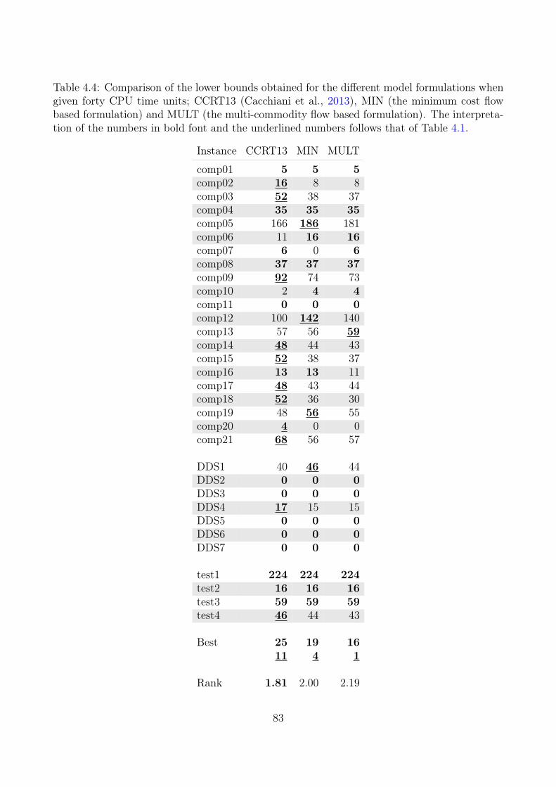
Table 4.4: Comparison of the lower bounds obtained for the different model formulations whengiven forty CPU time units; CCRT13 (Cacchiani et al., 2013), MIN (the minimum cost flowbased formulation) and MULT (the multi-commodity flow based formulation). The interpreta-tion of the numbers in bold font and the underlined numbers follows that of Table 4.1.

Instance CCRT13 MIN MULT

comp01 5 5 5comp02 16 8 8comp03 52 38 37comp04 35 35 35comp05 166 186 181comp06 11 16 16comp07 6 0 6comp08 37 37 37comp09 92 74 73comp10 2 4 4comp11 0 0 0comp12 100 142 140comp13 57 56 59comp14 48 44 43comp15 52 38 37comp16 13 13 11comp17 48 43 44comp18 52 36 30comp19 48 56 55comp20 4 0 0comp21 68 56 57

DDS1 40 46 44DDS2 0 0 0DDS3 0 0 0DDS4 17 15 15DDS5 0 0 0DDS6 0 0 0DDS7 0 0 0

test1 224 224 224test2 16 16 16test3 59 59 59test4 46 44 43

Best 25 19 1611 4 1

Rank 1.81 2.00 2.19

83

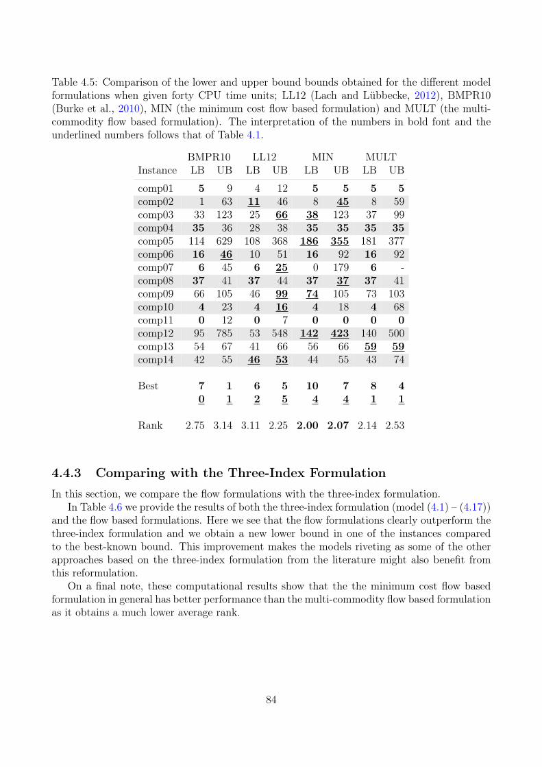
Table 4.5: Comparison of the lower and upper bound bounds obtained for the different modelformulations when given forty CPU time units; LL12 (Lach and Lübbecke, 2012), BMPR10(Burke et al., 2010), MIN (the minimum cost flow based formulation) and MULT (the multi-commodity flow based formulation). The interpretation of the numbers in bold font and theunderlined numbers follows that of Table 4.1.

BMPR10 LL12 MIN MULTInstance LB UB LB UB LB UB LB UB

comp01 5 9 4 12 5 5 5 5comp02 1 63 11 46 8 45 8 59comp03 33 123 25 66 38 123 37 99comp04 35 36 28 38 35 35 35 35comp05 114 629 108 368 186 355 181 377comp06 16 46 10 51 16 92 16 92comp07 6 45 6 25 0 179 6 -comp08 37 41 37 44 37 37 37 41comp09 66 105 46 99 74 105 73 103comp10 4 23 4 16 4 18 4 68comp11 0 12 0 7 0 0 0 0comp12 95 785 53 548 142 423 140 500comp13 54 67 41 66 56 66 59 59comp14 42 55 46 53 44 55 43 74

Best 7 1 6 5 10 7 8 40 1 2 5 4 4 1 1

Rank 2.75 3.14 3.11 2.25 2.00 2.07 2.14 2.53

4.4.3 Comparing with the Three-Index Formulation

In this section, we compare the flow formulations with the three-index formulation.In Table 4.6 we provide the results of both the three-index formulation (model (4.1) – (4.17))

and the flow based formulations. Here we see that the flow formulations clearly outperform thethree-index formulation and we obtain a new lower bound in one of the instances comparedto the best-known bound. This improvement makes the models riveting as some of the otherapproaches based on the three-index formulation from the literature might also benefit fromthis reformulation.

On a final note, these computational results show that the the minimum cost flow basedformulation in general has better performance than the multi-commodity flow based formulationas it obtains a much lower average rank.

84

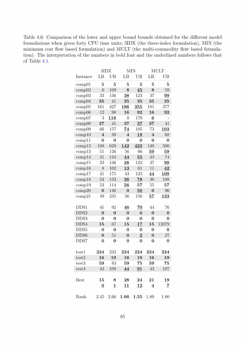
Table 4.6: Comparison of the lower and upper bound bounds obtained for the different modelformulations when given forty CPU time units; 3IDX (the three-index formulation), MIN (theminimum cost flow based formulation) and MULT (the multi-commodity flow based formula-tion). The interpretation of the numbers in bold font and the underlined numbers follows thatof Table 4.1.

3IDX MIN MULTInstance LB UB LB UB LB UB

comp01 5 5 5 5 5 5comp02 0 109 8 45 8 59comp03 33 136 38 123 37 99comp04 35 41 35 35 35 35comp05 161 427 186 355 181 377comp06 12 98 16 92 16 92comp07 3 118 0 179 6 -comp08 37 45 37 37 37 41comp09 66 157 74 105 73 103comp10 4 39 4 18 4 68comp11 0 0 0 0 0 0comp12 108 629 142 423 140 500comp13 51 126 56 66 59 59comp14 41 144 44 55 43 74comp15 33 136 38 123 37 99comp16 8 102 13 61 11 42comp17 41 175 43 123 44 109comp18 24 133 36 78 30 108comp19 53 114 56 57 55 57comp20 0 146 0 50 0 96comp21 49 235 56 156 57 133

DDS1 45 92 46 70 44 76DDS2 0 0 0 0 0 0DDS3 0 0 0 0 0 0DDS4 15 67 15 17 15 12079DDS5 0 0 0 0 0 0DDS6 0 51 0 2 0 27DDS7 0 0 0 0 0 0

test1 224 233 224 224 224 224test2 16 19 16 19 16 19test3 59 83 59 75 59 75test4 43 109 44 91 43 107

Best 15 8 28 24 21 190 1 11 12 4 7

Rank 2.45 2.66 1.66 1.55 1.89 1.80

85

4.5 PerspectivesWe proposed two mixed integer programming models for the curriculum based course timetablingproblem (CTT). We based both our models on network flow problems; the minimum cost flowproblem and the multi-commodity flow problem. These models are exact, meaning that theywill obtain optimal solutions given enough computational resources. We showed that thesemodels have far fewer integer variables than the standard three-index formulation for the CTT.By experimental results, we also showed that the models outperform the three-index formula-tion regarding finding feasible solutions when solved by a MIP solver.

Regarding lower bounds, the formulations are competitive with most of the mixed inte-ger programming based approaches from the literature and improve one of the currently bestknown lower bounds on the benchmarking instances from the second international timetablingcompetition.

Regarding upper bounds, the minimum cost flow based formulation performs better thanother state-of-the-art MIP based approaches.

Furthermore, some of the approaches from the literature are based on models similar to thethree-index formulation. Since we showed that our formulations outperform the three-indexformulation, we believe that these approaches can also benefit from adopting the proposednetwork flow formulations.

AcknowledgementsThe authors would like to thank Professor Stephan Røpke, Department of Management En-gineering, Technical University of Denmark, and Professor Carsten Thomassen, Departmentof Applied Mathematics and Computer Science, Technical University of Denmark for fruitfuldiscussions on the graphs and proofs. Niels-Christian Fink Bagger’s industrial PhD project isfunded by Innovation Fund Denmark (IFD). IFD has supported the work solely financially andhas not participated in any research related activities

ReferencesAhuja, R. K., Magnanti, T. L., and Orlin, J. B. (1993). Network Flows: Theory, Algorithms,

and Applications. Upper Saddle River, NJ, USA: Prentice-Hall, Inc. isbn: 0-13-617549-X.Bagger, N., Kristiansen, S., Sørensen, M., and Stidsen, T. (2015). “Flow Formulation-based

Model for the Curriculum-based Course Timetabling Problem”. In: MISTA 2015 Proceed-ings. Ed. by Z. Hanzálek, G. Kendall, B. McCollum, and P. S̆øucha. Proceedings of the 7thMultidisciplinary International Conference on Scheduling: Theory and Applications (MISTA2015), pp. 825–848.

Bettinelli, A., Cacchiani, V., Roberti, R., and Toth, P. (2015). “An overview of curriculum-basedcourse timetabling”. In: TOP, pp. 1–37.

Bonutti, A., De Cesco, F., Di Gaspero, L., and Schaerf, A. (2012). “Benchmarking curriculum-based course timetabling: Formulations, data formats, instances, validation, visualization,and results”. In: Annals of Operations Research 194.1, pp. 59–70.

86

Bron, C. and Kerbosch, J. (1973). “Algorithm 457: Finding All Cliques of an Undirected Graph”.In: Commun. ACM 16.9, pp. 575–577. issn: 0001-0782. doi: 10.1145/362342.362367. url:http://doi.acm.org/10.1145/362342.362367.

Burke, E. K., Mareček, J., Parkes, A. J., and Rudová, H. (2008). “Penalising Patterns in Timeta-bles: Novel Integer Programming Formulations”. In: Operations Research Proceedings 2007.Ed. by J. Kalcsics and S. Nickel. Vol. 2007. Operations Research Proceedings. 10.1007/978-3-540-77903-2_63. Springer Berlin Heidelberg, pp. 409–414. isbn: 978-3-540-77903-2.

Burke, E. K., Mareček, J., Parkes, A. J., and Rudová, H. (2010). “A supernodal formulation ofvertex colouring with applications in course timetabling”. In: Annals of Operations Research179.1, pp. 105–130.

Burke, E. K., Mareček, J., Parkes, A. J., and Rudová, H. (2012). “A branch-and-cut proce-dure for the Udine Course Timetabling problem”. In: Annals of Operations Research 194.1,pp. 71–87.

Cacchiani, V., Caprara, A., Roberti, R., and Toth, P. (2013). “A new lower bound for curriculum-based course timetabling”. In: Computers and Operation Research 40.10, pp. 2466–2477. doi:10.1016/j.cor.2013.02.010.

Di Gaspero, L., McCollum, B., and Schaerf, A. (2007). The Second International TimetablingCompetition (ITC-2007): Curriculum-based Course Timetabling (Track 3). Tech. rep. Schoolof Electronics, Electrical Engineering and Computer Science, Queenes University SARCBuilding, Belfast, United Kingdom.

Di Gaspero, L. and Schaerf, A. (2003). “Multi-neighbourhood Local Search with Applicationto Course Timetabling”. English. In: Practice and Theory of Automated Timetabling IV.Ed. by E. Burke and P. De Causmaecker. Vol. 2740. Lecture Notes in Computer Science.Springer Berlin Heidelberg, pp. 262–275. isbn: 978-3-540-40699-0. doi: 10.1007/978-3-540-45157-0_17. url: http://dx.doi.org/10.1007/978-3-540-45157-0_17.

Gurobi Optimization Inc. (2015). Gurobi Optimizer Reference Manual. url: http://www.gurobi.com.

Hao, J. K. and Benlic, U. (2011). “Lower bounds for the ITC-2007 curriculum-based coursetimetabling problem”. In: European Journal of Operational Research 212.3, pp. 464–472.

Kleinberg, J. and Tardos, E. (2005). Algorithm Design. Boston, MA, USA: Addison-WesleyLongman Publishing Co., Inc. isbn: 0321295358.

Lach, G. and Lübbecke, M. (2012). “Curriculum based course timetabling: new solutions toUdine benchmark instances”. In: Annals of Operations Research 194, pp. 255–272. issn:0254-5330.

Lach, G. and Lübbecke, M. E. (2008). “Optimal University Course Timetables and the Par-tial Transversal Polytope”. In: International Workshop on Experimental and Efficient Algo-rithms. Springer, pp. 235–248.

McCollum, B., Schaerf, A., Paechter, B., McMullan, P., Lewis, R., Parkes, A. J., Gaspero, L. D.,Qu, R., and Burke, E. K. (2010). “Setting the Research Agenda in Automated Timetabling:The Second International Timetabling Competition”. In: INFORMS Journal on Computing22.1, pp. 120–130.

87

5 Benders’ Decomposition forCurriculum-based Course Timetabling

Niels-Christian F. Baggera,b · Matias Sørensena,b · Thomas R. Stidsena

amORetime research group, Management Science, Department of Management Engineering,Technical University of Denmark, Produktionstorvet, Building 426B, DK-2800 Kgs. Lyngby,Denmark, http://www.moretime.man.dtu.dk/

bMaCom A/S, Vesterbrogade 48, 1., DK-1620 København V, Denmark

Status: Submitted to Computers & Operations Research

Abstract: In this paper we apply Benders’ decomposition to the Curriculum-based Course Timetabling (CTT) problem. The objective of the CTT problem is toassign a set of lectures to time slots and rooms. Our approach is based on splittingthe problem into a time scheduling problem and a room allocation problem. TheBenders’ algorithm is then used to generate cuts that connect the time scheduleand room allocation. We only generate feasibility cuts, meaning that most of thesolutions we obtain from a mixed integer programming solver are infeasible, andtherefore we also provide a heuristic to regain feasibility.

We compare our algorithm with other approaches from the literature on a totalof 32 data instances. We get a lower bound on 23 of the instances which are atleast as good as the lower bounds obtained by the state-of-the-art, and on eight ofthese our lower bounds are higher. On two of the instances, our lower bound is animprovement of the currently best-known. Lastly, we compare our decompositionwith the model without the decomposition on additionally six instances which aremuch larger than the other 32. To our knowledge, this is the first time that lowerbounds are calculated for these six instances.

Keywords: University Course Timetabling · Integer Programming · Benders’Decomposition · Maximum Flow · Minimum Cut

5.1 Curriculum-based Course TimetablingIn this work we consider the Curriculum based Course Timetabling Problem (CTT) introducedin track 3 of the second international timetabling competition (ITC2007) as described by Di

89

Gaspero et al. (2007), McCollum et al. (2010) and Bonutti et al. (2012). Most of the work onCTT focuses on finding high-quality solutions using heuristics. The drawback of these heuristicsis that they do not provide any proof of quality, e.g., how far from optimality the solutions are.We need bounding and exact methods to be able to validate the quality of the heuristics andnot much work has been put into developing these methods. In this article we apply Benders’decomposition to a Mixed Integer Programming (MIP) model that we presented in Baggeret al. (2016).

In the CTT problem we must schedule weekly lectures for multiple courses into time periodsand assign the lectures to rooms. We are given a set of days, each divided into a set oftime slots. We refer to a day and time slot combination as a period. The basic entities ofthe problem are the courses to schedule, and the periods and rooms that are available. Theproblem originates from a real world application and has received a lot of attention since thecompetition. Each course has a number of lectures which must all be scheduled in a periodand assigned a room. Furthermore all the lectures must be scheduled in distinct periods. Thisrequirement is referred to as the Lectures (L) constraint. The courses have specified some of theperiods to be unavailable periods, i.e., periods where it is not allowed to schedule the course.This requirement is referred to as the Availability (A) constraint. There are no constraintson assigning the courses to rooms, i.e., any course can be assigned to any room. Besides thecourses, periods and rooms the problem also contains lecturers and curricula, hence the nameCurriculum-based Course Timetabling. Each course is taught by a lecturer, and a curriculumis a set of courses which may be followed by the same students. If two courses are taught bythe same lecturer or belong to the same curriculum they cannot have lectures scheduled in thesame periods. This requirement is referred to as the Conflicts (C) constraint. For each room,at most one lecture can be assigned in any period, which is referred to as the Room Occupancy(RO) constraint. The objective of the CTT is to find a timetable which fulfils all the lattermentioned requirements, L, A, C and RO, while minimizing a weighted sum of the violationof four soft constraints; Room Capacity (RC), Room Stability (RStab), Minimum WorkingDays (MWD) and Isolated Lectures (IL). When a course is assigned to a room where thenumber of seats is smaller than the number of students that are attending the course thenthe constraint RC is violated by one for each student above the capacity of the room. It isdesired to assign lectures from the same course to as few distinct rooms as possible. A course isviolating constraint RStab by the total number of distinct rooms that it is assigned to minusone. The constraint MWD is the desire to spread lectures across a given number of days. Wesay that a day is a working day for a course if at least one lecture from the course is scheduledin a time slot on that day. For each course a number of minimum working days is providedand if the number of working days is below this number then the violation of the constraintis the difference. The last constraint IL is associated with the curricula. For each curriculumit is desired to have as few isolated lectures as possible. Each isolated lecture counts as oneviolation. A curriculum has an isolated lecture in a period if any of the courses belonging tothe curriculum has a lecture scheduled in the period and none of the courses have lecturesscheduled in the adjacent periods. We say that two periods are adjacent if they belong to thesame day and are in consecutive time slots.

In the following section 5.1.1 we provide an overview of other approaches applied to CTT. Insection 5.2 we first provide a brief introduction to Benders’ decomposition and then we describehow we apply it to CTT. In section 5.3 we describe a heuristic to repair partially infeasible

90

solutions, whereby partially infeasible we mean solutions where the time schedule is feasible,but not the room assignment. In section 5.4 we describe the computational results. Lastly, insection 5.5 we state our conclusions on this work.

5.1.1 Related Research

As we consider a MIP model for the problem, we mainly focus on other MIP based approachesin the literature. For a thorough overview of the problem and different approaches for CTT werefer to Bettinelli et al. (2015).

Burke et al. (2008) and Burke et al. (2010) introduces a compact MIP formulation thatis exact, in the sense that the optimal solution can be found by a generic MIP solver givenenough computational resources. However, many instances of the CTT cannot be solved for thisformulation within a reasonable time using a MIP solver and so Burke et al. (2010) proposemethods to derive lower and upper bounds. They obtain lower bounds by aggregating therooms into multi-rooms. For each multi-room the number of lectures that can be scheduled init in any period is equal to the umber of rooms that where aggregated. This problem providesa lower bound for CTT. To obtain an upper bound they fix the periods (or parts of them)according to the solution from the lower bounding mechanism and then assign rooms to thelectures. Burke et al. (2012) give an exact branch-and-cut algorithm which they also base onthe compact formulation, but some of the objective costs are left out and instead added ascuts during the solution process. This can be seen as a Benders’ decomposition, but instead ofgenerating the cuts dynamically they are generated a priori and then added when needed.

Lach and Lübbecke (2008) and Lach and Lübbecke (2012) proposed a method that dividesthe CTT into two stages. The started by grouping the rooms together such that if two roomshave the same capacity then they are in the same group. Then in the first stage, they scheduledthe courses into periods and assigned them to these capacities. This method is a Benders’Decomposition (Lübbecke, 2015). In the second stage, they assign the courses to the rooms,where the solution from the first stage is used to fix the courses at the determined periods andthe selected room capacities.

Hao and Benlic (2011) divides the MIP model that Lach and Lübbecke (2012) use in thefirst-stage into smaller parts by relaxing or removing some of the constraints. The relaxationsmakes it possible to decompose the model into a set of subproblems where they calculate alower bound for each subproblem. The sum of all these lower bounds is then a lower boundfor CTT. Cacchiani et al. (2013) present multiple extended MIP formulation, i.e., models withan exponential amount of variables. The approach that provides the best results divides theproblem into two parts; one focusing on the time scheduling related soft constraints and theother focusing on the room related soft constraints. They calculate a lower bound for each partand the sum of these lower bounds is then a lower bound for CTT.

In Bagger et al. (2016) two MIP models were presented that were inspired by Lach andLübbecke (2008) and Lach and Lübbecke (2012) and Burke et al. (2008) and Burke et al. (2010).The division of the problem described Lach and Lübbecke (2012) by was applied (excluding thenotion of distinct capacities) and it was shown that the two stages could be connected usingtwo underlying flow network formulations. The first formulation was based on a minimum costflow network and performed best of the two. The second formulation was based on a multi-commodity flow problem which is the formulation where we apply Benders’ decomposition

91

(Benders, 1962) in this article. The reason for using the last formulation, although it did notperform as well as the first, is that the underlying network is a feasibility problem. So we donot need to generate any optimality cuts, but only feasibility cuts.

5.2 Benders’ Decomposition

In this section we give an introduction to Benders’ decomposition followed by our applicationof the technique. Our introduction is a crude overview and we refer to (Benders, 1962) andMartin (1999, chapter 10) for a detailed description. We describe the method based on amodel containing two types of variables, x and y. The x variables are non-negative continuousvariables, and we do not have any assumptions on the y variables, i.e., x ≥ 0 and y ∈ Y whereY can be any domain, e.g., the set of integers. Consider the MIP model (5.1).

min c>x+ f(y)

s.t. Ax+B(y) ≥ b

y ∈ Yx ≥ 0

(5.1)

In model (5.1) c ∈ Rn is the cost vector of the x variables, A ∈ Rn×m is the constraint matrixof the x variables and b ∈ Rm is the right-hand-side vector of the constraints. f : Y → R issome function to evaluate the cost of the y variables and B is a vector function that evaluatesthe contribution of the y variables for the constraints. If we fix the y variables to some value inthe domain Y then what remains is a linear programme (LP). This assumption can be extendedas described by Geoffrion (1972), but we stick to the (LP) case in this context. Model (5.1)can be rewritten to model (5.2).

min f(y) + z

s.t. z ≥ minx≥0

{c>x |Ax ≥ b−B(y)

}y ∈ Yz ∈ R

(5.2)

In model (5.2) there is an inner optimization problem in the constraints. If the y variablesare fixed, then this is an LP and we can change it into its dual LP as in model (5.3).

min f(y) + z

s.t. z ≥ maxπ≥0

{(b−B(y))π |A>π ≤ c

}y ∈ Yz ∈ R

(5.3)

One interesting aspect of the inner optimization problem in model (5.3) is that the corre-sponding polytope is independent of the values of the y variables. So if the polytope

{ATπ ≤ c

}is non-empty then we can reformulate the problem using the extreme points Πp and extremerays Πr as in model (5.4).

92

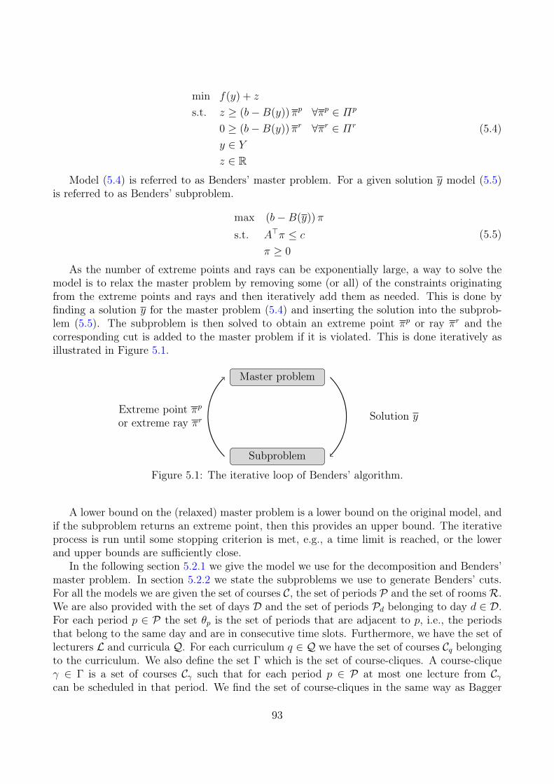
min f(y) + z

s.t. z ≥ (b−B(y))πp ∀πp ∈ Πp

0 ≥ (b−B(y))πr ∀πr ∈ Πr

y ∈ Yz ∈ R

(5.4)

Model (5.4) is referred to as Benders’ master problem. For a given solution y model (5.5)is referred to as Benders’ subproblem.

max (b−B(y))π

s.t. A>π ≤ c

π ≥ 0

(5.5)

As the number of extreme points and rays can be exponentially large, a way to solve themodel is to relax the master problem by removing some (or all) of the constraints originatingfrom the extreme points and rays and then iteratively add them as needed. This is done byfinding a solution y for the master problem (5.4) and inserting the solution into the subprob-lem (5.5). The subproblem is then solved to obtain an extreme point πp or ray πr and thecorresponding cut is added to the master problem if it is violated. This is done iteratively asillustrated in Figure 5.1.

Master problem

Subproblem

Solution yExtreme point πpor extreme ray πr

Figure 5.1: The iterative loop of Benders’ algorithm.

A lower bound on the (relaxed) master problem is a lower bound on the original model, andif the subproblem returns an extreme point, then this provides an upper bound. The iterativeprocess is run until some stopping criterion is met, e.g., a time limit is reached, or the lowerand upper bounds are sufficiently close.

In the following section 5.2.1 we give the model we use for the decomposition and Benders’master problem. In section 5.2.2 we state the subproblems we use to generate Benders’ cuts.For all the models we are given the set of courses C, the set of periods P and the set of rooms R.We are also provided with the set of days D and the set of periods Pd belonging to day d ∈ D.For each period p ∈ P the set θp is the set of periods that are adjacent to p, i.e., the periodsthat belong to the same day and are in consecutive time slots. Furthermore, we have the set oflecturers L and curricula Q. For each curriculum q ∈ Q we have the set of courses Cq belongingto the curriculum. We also define the set Γ which is the set of course-cliques. A course-cliqueγ ∈ Γ is a set of courses Cγ such that for each period p ∈ P at most one lecture from Cγcan be scheduled in that period. We find the set of course-cliques in the same way as Bagger

93

et al. (2016). For each course c ∈ C we have the number of lectures that needs to be scheduledLc ∈ Z+, where Z+ is the set of non-negative integers, and the minimum number of requestedworking daysMc ∈ Z+. We also have the number of students attending the course Sc ∈ Z+ andfor each period p ∈ P the parameter Fc,p ∈ B specifying whether or not it is feasible to schedulec in p. For each room, we have the parameter Cr ∈ Z+ which is the capacity of the room. Wehave WMWD ∈ R+, W IL ∈ R+, WRC ∈ R+ and WRStab ∈ R+ which are the non-negativeweights of the soft constraints, MWD, IL, RC and RStab respectively. Lastly, for any valuex ∈ R we use the notation (x)+ to denote that we are taking the maximum of x and zero.

5.2.1 Master Problem

The model we use for the decomposition is the multi-commodity flow formulation that wepresented in Bagger et al. (2016). We start by describing this model, and then we describe howwe reformulate it using Benders’ decomposition.

For each course c ∈ C and period p ∈ P there is a binary variable xc,p which is set to oneif c is scheduled in p and zero otherwise. To calculate the violation of the requested minimumworking days we need to calculate which days the courses are scheduled to. We define a binaryvariable tc,d for each course c ∈ C and day d ∈ D which is set to one if c is scheduled in at leastone of the periods Pd and zero otherwise. Let wc for each course c ∈ C be an integer variablecounting the number of days, below the minimum requested, that c has lectures scheduled.Lastly for each curriculum q ∈ Q and period p ∈ P there is a binary variable sq,p that is setto one if q has an isolated lecture in p and zero otherwise. We can then formulate the timescheduling part of the problem as follows:

∑p∈P

xc,p = Lc ∀c ∈ C (5.6)

xc,p ≤ Fc,p ∀c ∈ C, p ∈ P (5.7)∑c∈Cγ

xc,p ≤ 1 ∀γ ∈ Γ, p ∈ P (5.8)

∑p∈Pd

xc,p ≥ tc,d ∀c ∈ C, d ∈ D (5.9)∑d∈D

tc,d + wc ≥Mc ∀c ∈ C (5.10)

∑c∈Cq

xc,p −∑p′∈θp

xc,p′

≤ sq,p ∀q ∈ Q, p ∈ P (5.11)

xc,p ∈ B ∀c ∈ C, p ∈ P (5.12)tc,d ∈ B ∀c ∈ C, d ∈ D (5.13)wc ∈ Z+ ∀c ∈ C (5.14)sq,p ∈ B ∀q ∈ Q, p ∈ P (5.15)

Constraints (5.6) and (5.7) ensure that all lectures are scheduled, that they are scheduled indifferent periods and that they are only scheduled in the periods where the courses are available.

94

Constraints (5.8) ensure that at most one lecture from each course-clique is scheduled in everyperiod. The violation of the MWD constraint is calculated in (5.9) and (5.10). Lastly, theconstraints (5.11) calculate in which periods the curricula have isolated lectures. The domainsof the variables are given in (5.12) – (5.15).

For the room assignment part of the problem we define an integer variable yc,r for eachcourse c ∈ C and room r ∈ R which counts the number of times that c has been assigned tor. zc,r is a binary variable that is set to one if course c ∈ C is assigned to room r ∈ R at leastonce and zero otherwise. The room assignment part can then be formulated as follows:

∑r∈R

yc,r = Lc ∀c ∈ C (5.16)

yc,r ≤ Lczc,r ∀c ∈ C, r ∈ R (5.17)yc,r ≥ zc,r ∀c ∈ C, r ∈ R (5.18)∑r∈R

zc,r ≥ 1 ∀c ∈ C, r ∈ R (5.19)

yc,r ∈ Z+ ∀c ∈ C, r ∈ R (5.20)zc,r ∈ B ∀c ∈ C, r ∈ R (5.21)

Constraints (5.16) ensure that all lectures is assigned a room. For every course c ∈ C androom r ∈ R the variable yc,r must be set to zero if zc,r is zero and it must be set to a positivevalue if zc,r is set to one. This is ensured by the constraints (5.17) and (5.18). Since everylecture must be scheduled, then every course must be assigned to at least one room which isreflected by the constraints (5.19). The domains of the variables are given in (5.20) – (5.21).

Finally, from the two parts; (5.6) – (5.15) and (5.16) – (5.21), we can formulate the objectivefunction which is to be minimized:

o (x, y, z):=WMWD∑c∈C

wc

+WRC∑

c∈C,r∈R(Sc − Cr)

+yc,r

+WRStab∑c∈C

(∑r∈R

zc,r − 1

)+W IL

∑q∈Q,p∈P

sq,p (5.22)

Until now, we have given the time scheduling and room assignment part of the problem asseparate parts. Given a binary variable fc,p,r for each course c ∈ C, period p ∈ P and roomr ∈ R, which is set to one if c is scheduled in room r at period p, the two parts can be connectedas follows:

95

∑p∈P

fc,p,r = yc,r ∀c ∈ C, r ∈ R (5.23)∑r∈R

fc,p,r ≤ xc,p ∀c ∈ C, p ∈ P (5.24)∑c∈C

fc,p,r ≤ 1 ∀r ∈ R, p ∈ P (5.25)

fc,p,r ∈ B ∀c ∈ C, p ∈ P , r ∈ R (5.26)

We show in Bagger et al. (2016) that the integrality requirements (5.26) can be relaxed tonon-negativity constraints such that the f variables are continuous. This means that we canproject them out and replace (5.23) – (5.26) by the following Benders’ cuts:

∑c∈C,p∈P

αkc,pxc,p +∑

c∈C,r∈R

βkc,ryc,r ≤ ηk ∀k ∈ K (5.27)

The set K is the set of Benders’ cuts. For each cut k ∈ K the coefficient of the variablexc,p is αkc,p for each course c ∈ C and p ∈ P , and for each course c ∈ C and room r ∈ R thecoefficient of the variable yc,r is βkc,r. The parameter ηk is a constant for each k ∈ K. Since Kcan be exponentially large we add the cuts dynamically when needed. We add some of the cutsstatically. For instance, we cannot schedule more courses to a single period than the numberof rooms available: ∑

c∈C

xc,p ≤ |R| ∀p ∈ P (5.28)

Similarly the total number of times that some room is assigned to by the courses cannotexceed the total number of periods:∑

c∈C

yc,r ≤ |P| ∀r ∈ R (5.29)

The cuts (5.28) and (5.29) are added to the master problem before we start the solutionprocess, and we generate the remaining cuts when an integer solution violates them.

5.2.2 Subproblems

In this section, we describe the subproblems. Our first subproblem is based on the problemconnecting the x and y variables (5.23) – (5.26). These cuts are necessary and sufficient toensure that the solutions obtained in our decomposed model are equivalent to the solutionsin our non-decomposed model. We base the second subproblem on the indirect connectionbetween the x and z variables. The applicability of the second subproblem is to generate cutson the z variables as they are connected with the y in the constraints (5.17) and (5.18) so thecuts will also have an indirect affect on the y variables.

96

5.2.2.1 Dual LP

The first subproblem we use, directly follows from the LP relaxation of (5.23) – (5.26), as it wasmentioned before that the integrality constraints can be neglected. Given a solution (x, y, z)we fix the x and y variables and if (5.23) – (5.26) is infeasible then we need to identify a cut.It can be verified that due to constraints (5.6) and (5.16) if we remove constraints (5.25) thenthe problem is feasible. So to find out if (5.23) – (5.26) is infeasible for the given solution, wesubtract a non-negative variable u from the left-hand-side of each of the constraints (5.25). Wethen search for the solution that minimizes u:

min u (5.30)

s.t.∑p∈P

fc,p,r = yc,r ∀c ∈ C, r ∈ R (5.31)∑r∈R

fc,p,r = xc,p ∀c ∈ C, p ∈ P (5.32)∑c∈C

fc,p,r − u ≤ 1 ∀r ∈ R, p ∈ P (5.33)

fc,p,r ≥ 0 ∀c ∈ C, p ∈ P , r ∈ R (5.34)u ≥ 0 (5.35)

Note that we have changed the inequality (5.24) into the equality (5.32). This is becauseany solution

(x, y, z, f

)that is feasible must meet equality in the constraints (5.24), since

Lc =∑

r∈R yc,r =∑

p∈P,r∈R f c,p,r ≤∑

p∈P xc,p = Lc must hold for each c ∈ C. The problem(5.23) – (5.26) is feasible for the given solution (x, y, z) if and only if there exists a solutionfor (5.30) – (5.35) where the variables x and y are fixed at the values x and y respectively andwhere the value of u is zero. We can, therefore, use this problem to generate feasibility cuts.

Given a solution (x, y, z), we fix the variables x and y in (5.30) – (5.35) to the values x andy, i.e., setting the bounds x ≤ x ≤ x and y ≤ y ≤ y, and solve the problem to optimality. Letrxc,p and ryc,r be the reduced costs of the variables x and y respectively and let u be the value ofthe variable u. According to Fischetti (2015) we can derive the Benders’ cut as follows:∑

c∈C,p∈P

rxc,p (xc,p − xc,p) +∑

c∈C,r∈R

ryc,r(yc,r − yc,r

)+ u ≤ 0 (5.36)

We add the cut (5.36) whenever it is violated by an integer solution (x, y, z).

5.2.2.2 Maximum Flow / Minimum Cut

In the previous section we described how to obtain the cuts from (5.23) – (5.26). Those cutsonly connect the x and y variables together. In this section, we look at the link between thex and z variables. Though they are not directly connected in any constraints, they have anindirect relation since the y and z variables are contained in some of the same constraints.Consider the model (5.23) – (5.26). It can be shown that the constraints (5.24) must be metby equality in any feasible solution. When changing the inequality in (5.24) into an equality,

97

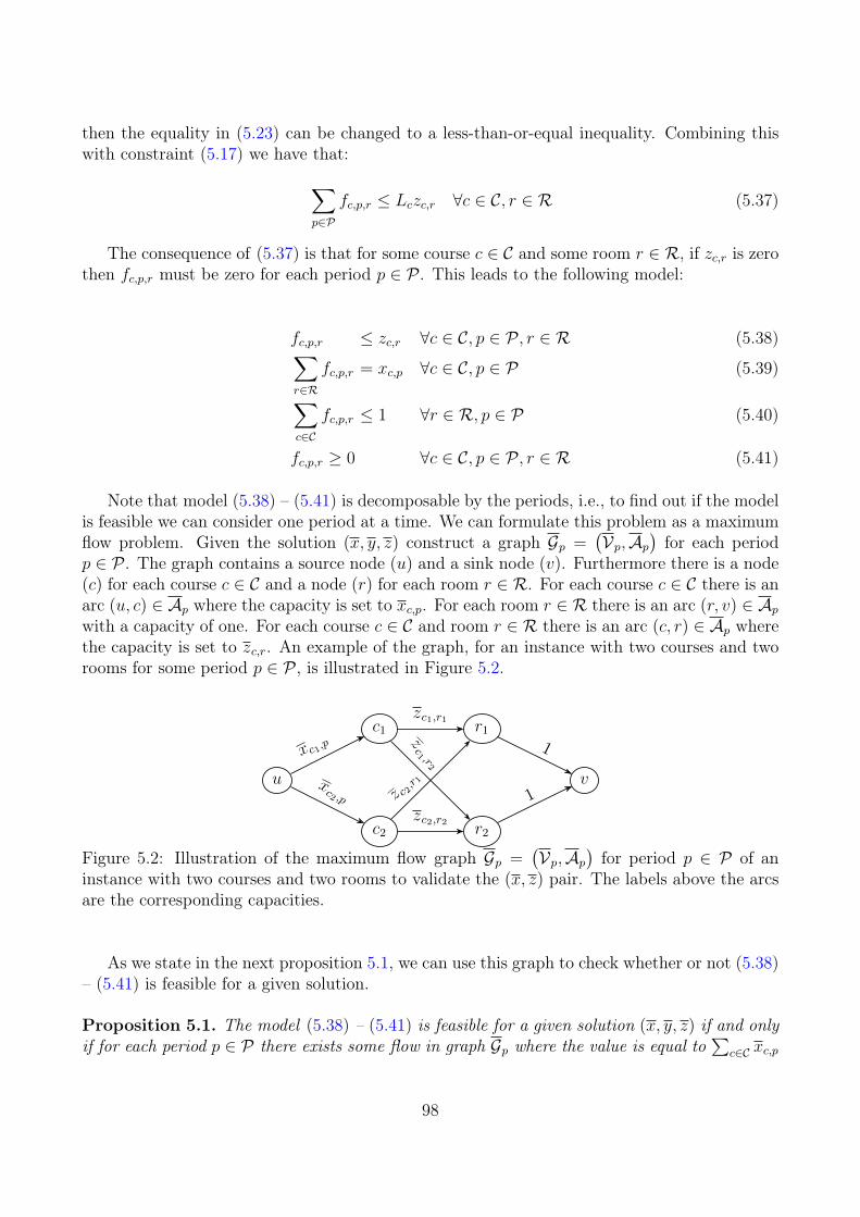
then the equality in (5.23) can be changed to a less-than-or-equal inequality. Combining thiswith constraint (5.17) we have that:∑

p∈P

fc,p,r ≤ Lczc,r ∀c ∈ C, r ∈ R (5.37)

The consequence of (5.37) is that for some course c ∈ C and some room r ∈ R, if zc,r is zerothen fc,p,r must be zero for each period p ∈ P . This leads to the following model:

fc,p,r ≤ zc,r ∀c ∈ C, p ∈ P , r ∈ R (5.38)∑r∈R

fc,p,r = xc,p ∀c ∈ C, p ∈ P (5.39)∑c∈C

fc,p,r ≤ 1 ∀r ∈ R, p ∈ P (5.40)

fc,p,r ≥ 0 ∀c ∈ C, p ∈ P , r ∈ R (5.41)

Note that model (5.38) – (5.41) is decomposable by the periods, i.e., to find out if the modelis feasible we can consider one period at a time. We can formulate this problem as a maximumflow problem. Given the solution (x, y, z) construct a graph Gp =

(Vp,Ap

)for each period

p ∈ P . The graph contains a source node (u) and a sink node (v). Furthermore there is a node(c) for each course c ∈ C and a node (r) for each room r ∈ R. For each course c ∈ C there is anarc (u, c) ∈ Ap where the capacity is set to xc,p. For each room r ∈ R there is an arc (r, v) ∈ Apwith a capacity of one. For each course c ∈ C and room r ∈ R there is an arc (c, r) ∈ Ap wherethe capacity is set to zc,r. An example of the graph, for an instance with two courses and tworooms for some period p ∈ P , is illustrated in Figure 5.2.

c1

c2

u

r1

r2

v

xc1,p

xc2 ,p

zc1,r1

zc1 ,r

2

z c 2,r 1

zc2,r2

1

1

Figure 5.2: Illustration of the maximum flow graph Gp =(Vp,Ap

)for period p ∈ P of an

instance with two courses and two rooms to validate the (x, z) pair. The labels above the arcsare the corresponding capacities.

As we state in the next proposition 5.1, we can use this graph to check whether or not (5.38)– (5.41) is feasible for a given solution.

Proposition 5.1. The model (5.38) – (5.41) is feasible for a given solution (x, y, z) if and onlyif for each period p ∈ P there exists some flow in graph Gp where the value is equal to

∑c∈C xc,p

98

Proof of proposition 5.1. Consider the solution (x, y, z) and the graph Gp for some period p ∈ P .We first prove that if the model is feasible for the period, then there exists some flow in thegraph where the value of the flow is equal to

∑c∈C xc,p. We then prove that if there exists

some flow in the graph where the value of the flow is equal to∑

c∈C xc,p then there is a feasiblesolution for the model for the period.

Consider some solution f to the model (5.38) – (5.41) for (x, y, z). Consider the graph Gp forsome period p ∈ P . For each course c ∈ C and room r ∈ R the amount of flow we send on thepath (u) → (c) → (r) → (v) is equal to f c,p,r. To validate that this is a flow for the graph weneed to check if the node balancing constraints and the capacity constraints are met. Since weare only sending flow on paths from the source to the sink, then the node balancing constraintsmust be met. The flow leaving node (c) is equal to

∑r∈R f c,p,r and due to the node balancing

constraints and the constraints (5.39) then the flow on the arc (u, c) must be equal xc,p whichis the capacity of that arc. The flow on the arc (c, r) is f c,p,r and due to constraint (5.38) thisis less than or equal to zc,r which is the capacity on the arc. The total amount of flow enteringnode (r) is equal to

∑c∈C f c,p,r and due to the node balancing constraints then the flow on the

arc (r, v) must be equal to this value. Because of the constraint (5.40) the flow on the arc (r, v)must, therefore, be less than or equal to one which is the capacity of the arc. The value ofthe flow must be equal to

∑c∈C xc,p because of the constraints (5.39). So if (5.38) – (5.41) is

feasible for the given solution then there is a flow for the graph where the value of the flow is∑c∈C xc,p.Now consider some flow for the graph Gp for period p ∈ P where the value of the flow is

equal to∑

c∈C xc,p. For each course c ∈ C and room r ∈ R let f c,p,r denote the amount of flowon the arc (c, r). f is a feasible solution for the f variables if the constraints (5.38) – (5.40) arenot violated. Since the capacity on the arc (c, r) for course c ∈ C and room r ∈ R is zc,r thenthe constraints (5.38) cannot be violated. Since the sum of the capacities leaving the sourcenode is equal to

∑c∈C xc,p then this means that the flow on arc (u, c) for each course c ∈ C must

be equal to xc,p and due to the node balancing constraints then all the flow leaving (c) mustalso equal this value, i.e.,

∑r∈R f c,p,r must be equal to xc,p, meaning that the constraints (5.39)

are fulfilled. The total amount of flow entering node (r) must be equal to∑

c∈C f c,p,r anddue to the node balancing constraints this value cannot exceed one, which means that theconstraints (5.40) are not violated. So if there exists some flow for the graph where the valueof the flow is equal to

∑c∈C xc,p then the model is feasible.

Since we considered an arbitrary period, then this concludes our proof of proposition 5.1.

For the source node (u) and sink node (v) a u − v cut is a cut that separates the graphinto two parts; the u side containing the source node, and the v side containing the sink node.For the maximum flow problem, the value of any flow in the graph is upper bounded by thesum of the capacities for any u− v cut (Ahuja et al., 2013, property 6.1). In the remainder ofthe section whenever we mention a cut we mean a u − v cut unless specified otherwise. If weconsider some cut χp ⊆ Ap in the graph Gp then the sum of the capacities in the cut must begreater than or equal to

∑c∈C xc,p for the solution to be feasible. So given the solution (x, y, z)

we solve the maximum flow problem by the labeling algorithm described by Ahuja et al. (2013,chapter 6). This algorithm also finds a minimum cut χp ⊆ Ap and if the value of the maximumflow (capacity of the minimum cut) is less than

∑c∈C xc,p we add the following cut to the master

problem:

99

∑(u,c)∈χp

xc,p +∑

(c,r)∈χp

zc,r +∣∣(r, v) ∈ χp

∣∣ ≥ ∑(u,c)∈Ap

xc,p (5.42)

For ease of notation in (5.42) we write (u, c) ∈ A which means; for each c ∈ C where thearc (u, c) is in the set A. Similarly, (r, v) ∈ A means for each room r ∈ R where the arc (r, v)is in the set A and (c, r) ∈ A is the set of all the arcs (c, r) for each c ∈ C and r ∈ R in theset A. We use the notation | · | on these sets to denote the cardinalities. We use this notationthroughout the remainder of the paper.

We can rewrite (5.42) into a simpler form:∑(u,c)∈Ap\{χp}

xc,p −∑

(c,r)∈χp

zc,r ≤∣∣(r, v) ∈ χp

∣∣ (5.43)

Whenever we get an integer solution (x, y, z) we add the cut (5.43) for each period p ∈ Pwhere it is violated.

5.3 Primal Heuristic

The solutions obtained are often infeasible during the Branch-and-Bound process, which meansthat it is hard for the MIP solver to achieve upper bounds used for pruning. Therefore, we haveimplemented a heuristic to regain feasibility whenever a cut is generated to help the solver. Inthe heuristic we exploit the property that the courses can be assigned to any room. Due toconstraints (5.28) we know that given any solution (x, y, z) the time-schedule part x of thesolution is feasible, meaning that it is possible to create a room assignment based in the time-schedule to obtain a complete solution. The heuristic runs through every period and in eachperiod the lectures that are scheduled in that period are each assigned to a distinct room. Thiswill always be possible since no more courses are scheduled in any period than the number ofrooms available. Based on this assignment we then calculate the values of the y and z variables.

For each period p ∈ P we find a minimum cut χp in the graph Gp as described in sec-tion 5.2.2.2. Then we calculate the value vp

(χp):

vp(χp)

:=∑

(u,c)∈Ap\{χp}xc,p −

∑(c,r)∈χp

zc,r −∣∣(r, v) ∈ χp

∣∣ (5.44)

If vp(χp)> 0 then we cannot schedule all lectures in p and we need to change the values of

the z variables to obtain feasibility. We do this by ordering the periods according to the valuesof vp

(χp)from the largest to the smallest. We then iterate over the periods in the given order

and for each period p ∈ P we perform the following steps:

1. Let the graph Gp be defined as in section 5.2.2.2 with the same capacities. For each coursec ∈ C and room r ∈ R let the weight on the arc (c, r) ∈ Ap be WRC (Sc − Cr)+ and letthe weights of the remaining arcs be zero.

2. If vp(χp)≤ 0, then stop.

100

3. For every arc (c, r) ∈ χp, if zc,r (the capacity) is zero then we open the room, i.e., wechange the value to one.

4. We then find the minimum cost maximum flow f (minimum cut χp) and for every arc(c, r) were we changed the capacity in step 3, if there is no flow on the arc, i.e., if f c,p,r = 0,we change the capacity back to zero.

5. Given the new minimum cut χp, update the value vp(χp)and go back to step 2.

When we have processed all periods we set the values y as follows:

yc,r =∑p∈P

f c,p,r c ∈ C, p ∈ P , r ∈ R (5.45)

We then set the z values as follows to ensure that the constraints (5.18) are fulfilled:

zc,r =

{1 if yc,r > 0

0 otherwisec ∈ C, p ∈ P , r ∈ R (5.46)

In step 3 we solve a minimum cost maximum flow problem, which is to find a minimum-costflow among all the maximum flows. The reason we are solving a minimum cost maximum flowproblem instead of just a maximum flow problem is that we want to create a feasible solutionwithout increasing the penalty of the RStab constraint too much. The algorithm we use isa modified version of the algorithm described by Ahuja et al. (2013, section 9.7) which findsthe minimum cost flow given the demands and supplies on the nodes. We have a supply onthe source node and a demand on the sink node both equal to

∑c∈C xp and on the rest of the

nodes, the demands and supplies are zero. The modification to the algorithm is the stoppingcriterion. In its pure form the algorithm assumes that there it is possible to meet all demandsof the nodes. Since we do not always have a feasible flow, we add the stopping criterion that ifno path exists from the source node to the sink node in the residual graph, then the algorithmmust stop. So the modified algorithm finds the minimum cost flow among all the maximumflows that exists. We can find the minimum cut from this flow in the same way as we did insection 5.2.2.2.

We need to show that the algorithm is finite and returns a feasible solution. If the algorithmassigns all lectures to rooms in each period, then the overall solution is feasible. So we needonly to show that the algorithm is finite and returns a feasible solution for a single period sincethere is a finite number of periods. For period p ∈ P , if all the arcs (c, r) ∈ Ap have a capacityof one then all lectures scheduled in the period can be assigned to a room. So if the period isinfeasible then some of the arcs (c, r) ∈ Ap must have a capacity of zero. As long as at least oneof the lectures cannot be assigned a room, i.e., as long as vp

(χp)> 0, the algorithm changes

at least one value zc,r from zero to one for some arc (c, r) in each iteration, assuming step 3 iscorrect. The correctness of step 3 is given by proposition 5.2. Since there is a finite number ofthese arcs, then the algorithm must also be finite. Furthermore, since the algorithm does notstop as long as vp

(χp)> 0 then the solution will also be feasible, for the period p ∈ P , since

all capacities on the arcs (c, r) ∈ Ap are set to one in the worst case.

101

Proposition 5.2. For a solution (x, y, z), a period p ∈ P and a minimum cut χp, if vp(χp)> 0

then there must exist a course c ∈ C and room r ∈ R where the arc (c, r) is in the cut χp andthe capacity is zero, i.e., zc,r = 0

To prove proposition 5.2 we first prove that in the minimum cut χp, at least one of the arcs(c, r) ∈ Ap must be in the cut. Afterwards, we prove that the arcs (c, r) ∈ χp cannot all havea capacity of one.

Proof. At least one arc (c, r) ∈ Ap is in the cut χp. We begin the proof by showing that not allthe arcs (u, c) ∈ Ap can be in the minimum cut χp nor can all the arcs (r, v) ∈ Ap. In Figure 5.3we give an illustration of the graph Gp and two cuts; χ1

p and χ2p.

c1

c2

u

r1

r2

v

xc1,p

xc2 ,p

zc1,r1

zc1 ,r

2

z c 2,r 1

zc2,r2

1

1

χ1p χ2

p

Figure 5.3: Illustration of the two cuts; cut χ1p containing all arcs leaving the source node and

χ2p containing all arcs entering the sink node.

The cut χ1p contains all the arcs (u, c) ∈ Ap and the cut χ2

p contains all the arcs (r, v) ∈ Ap.Since we know vp

(χp)< 0 for the minimum cut χp then neither χ1

p nor χ2p can be a minimum

cut. The reason that χ1p cannot be a minimum cut is that the total capacity of the minimum

cut χp is strictly less than∑

c∈C xc,p, however, since the cut χ1p contains all the arcs (u, c) ∈ Ap

then the total capacity of χ1p must be greater than or equal to

∑c∈C xc,p. The reason that

χ2p cannot be a minimum cut is that

∑c∈C xc,p ≤ |R| due to constraint (5.28) thus the total

capacity of the minimum cut χp is strictly less than |R| since not all lectures are assigned to aroom, however, since the cut χ2

p contains all the arcs (r, v) ∈ Ap then the total capacity of χ2p

must be greater than or equal to |R|.As we cannot have all arcs (u, c) ∈ Ap in the minimum cut then there must exist some

course c ∈ C where the node (c) is on the same side of the cut as the source node (u). Similarly,as we cannot have all arcs (r, v) ∈ Ap in the minimum cut then there must exist some roomr ∈ R where the node (r) is on the same side of the cut as the sink node (v). Hence, the arc(c, r) must be in the cut which concludes our proof.

We have shown that at least one of the arcs (c, r) ∈ Ap must be in the minimum cut. Oneside effect of our proof is that since not all of the arcs (u, c) ∈ Ap can be in the cut then wehave the following: ∣∣(u, c) ∈ χp∣∣ ≤ |C| − 1 (5.47)

102

Similarly, since not all the arcs (r, v) ∈ Ap can be in the minimum cut then we have thefollowing: ∣∣(r, v) ∈ χp

∣∣ ≤ |R| − 1 (5.48)

Before the next proof, we make the assumption that |R| ≥ 2. It is fair to make thisassumption since if |R| = 0 the problem is infeasible and if |R| = 1 then at most one course isscheduled in each period and can be assigned to whichever room it has selected.

Proof. zc,r = 0 for at least one arc (c, r) ∈ χp. We showed in the previous proof that there isat least one arc (c, r) in the minimum cut for some course c ∈ C and room r ∈ R. Now weshow for at least one of the arcs (c, r) ∈ χp the capacity is zero. To prove this, we assume thatevery arc (c, r) ∈ χp has a capacity of one and show that this leads to a contradiction.

Since we consider an infeasible solution then due to constraint (5.43) the following musthold: ∑

(c,r)∈χp

zc,r +∣∣(r, v) ∈ χp

∣∣ < ∑(u,c)∈Ap\χp

xc,p (5.49)

All capacities in the graph are either zero or one and so we can calculate an upper boundof the right-hand side of (5.49) as follows:∑

(u,c)∈Ap\χp

xc,p ≤∣∣(u, c) ∈ Ap\χp∣∣ = |C| −

∣∣(u, c) ∈ χp∣∣ (5.50)

If we insert (5.50) into (5.49) together with our assumption that the capacities of all thearcs (c, r) ∈ χp are one then we get the following:∣∣(c, r) ∈ χp∣∣+

∣∣(r, v) ∈ χp∣∣ < |C| − ∣∣(u, c) ∈ χp∣∣ (5.51)

Consider an arc (c, r) for some course c ∈ C and some room r ∈ R. For this arc to be in thecut, the node (c) must be on the same side of the cut as the source node and the node (r) mustbe on the same side as the sink node. The node (c) is on the source side if and only if the arc(u, c) is not in the cut. Similarly, the node (r) is on the sink side if and only if the arc (r, v) isnot in the cut. So we can express

∣∣(c, r) ∈ χp∣∣ as the product of the arcs (u, c) and (r, v) thatare not in the cut: ∣∣(c, r) ∈ χp∣∣ =

∣∣(u, c) ∈ Ap\χp∣∣ ∣∣(r, v) ∈ Ap\χp∣∣ (5.52)

We can rewrite (5.52) by noting that the number of arcs leaving the source that are not inthe cut is equal to the number of arcs leaving the source minus the arcs in the cut, and similarlyfor the arcs entering the sink:∣∣(c, r) ∈ χp∣∣ =

(|C| −

∣∣(u, c) ∈ χp∣∣) (|R| − ∣∣(r, v) ∈ χp∣∣) (5.53)

Expanding the expression gives us the following:

∣∣(c, r) ∈ χp∣∣ =|C||R|+∣∣(u, c) ∈ χp∣∣ ∣∣(r, v) ∈ χp

∣∣− |R|

∣∣(u, c) ∈ χp∣∣− |C| ∣∣(r, v) ∈ χp∣∣ (5.54)

103

Substituting (5.54) into (5.51) gives the following:

|C||R|+∣∣(r, v) ∈ χp

∣∣ < |C| − ∣∣(u, c) ∈ χp∣∣ ∣∣(r, v) ∈ χp∣∣

+ |R|∣∣(u, c) ∈ χp∣∣+ |C|

∣∣(r, v) ∈ χp∣∣− ∣∣(u, c) ∈ χp∣∣ (5.55)

Next we rearrange the terms:

|C| (|R| − 1) < (|C| − 1) (|R| − 1)

−((|R| − 1)−

∣∣(r, v) ∈ χp∣∣) ((|C| − 1)−

∣∣(u, c) ∈ χp∣∣) (5.56)

An upper bound can be found for the right-hand side of (5.56) by finding a lower bound forthe expression: (

(|R| − 1)−∣∣(r, v) ∈ χp

∣∣) ((|C| − 1)−∣∣(u, c) ∈ χp∣∣) (5.57)

Since we know that∣∣(r, v) ∈ χp

∣∣ ≤ |R| − 1 then((|R| − 1)−

∣∣(r, v) ∈ χp∣∣) ≥ 0 must hold.

Similarly((|C| − 1)−

∣∣(u, c) ∈ χp∣∣) ≥ 0 must also hold which means that the minimum valuethat (5.57) can take must be zero. So the right-hand side of (5.56) must be less than or equalto (|C| − 1) (|R| − 1) and since we assume |R| ≥ 2 we can divide with |R| − 1 and we get thefollowing:

|C| < |C| − 1 (5.58)

As (5.58) is a contradiction then we have concluded our proof and at least one of the arcs(c, r) ∈ χp must have a capacity of zero.

We have now proven that our algorithm is finite and returns a feasible solution. We runthis heuristic whenever we retrieve an integer solution where a cut is generated.

5.4 Computational ExperimentsIn this section, we report our computational experiments. We conducted all our tests on a3.40GHz Intel® Core™ processor running Windows 10 with 8GB memory RAM.We used Gurobi6.5.2 provided by Gurobi Optimization Inc. (2015) both for the master problem and also forthe subproblem described in section 5.2.2.1. We set all parameters in Gurobi to their defaultexcept, Presolve , Threads and LazyConstraints. We set Presolve to 2 (the most aggressivelevel), Threads to 1 as this was the maximum allowed threads for the ITC2007 competitionand LazyConstraints to 1 to be able to add cuts on integer solutions.

We tested our approach on four datasets; TEST, COMP, DDS and ERLANGEN. TheTEST dataset consists of four data instances, test1 – test4, proposed by Di Gaspero andSchaerf (2003). The COMP dataset contains 21 data instances, comp01 – comp21, describedin Di Gaspero et al. (2007) mainly taken from the University of Udine. The DDS datasetcontains seven data instances, DDS1 – DDS7, taken from other Italian universities. The ER-LANGEN dataset consists of six instances, erlangen2012_1, erlangen2012_2, erlangen2013_1,

104

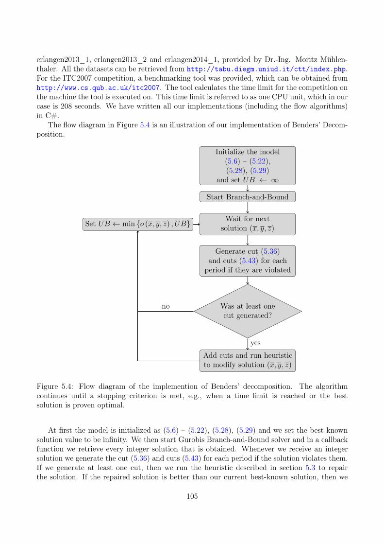
erlangen2013_1, erlangen2013_2 and erlangen2014_1, provided by Dr.-Ing. Moritz Mühlen-thaler. All the datasets can be retrieved from http://tabu.diegm.uniud.it/ctt/index.php.For the ITC2007 competition, a benchmarking tool was provided, which can be obtained fromhttp://www.cs.qub.ac.uk/itc2007. The tool calculates the time limit for the competition onthe machine the tool is executed on. This time limit is referred to as one CPU unit, which in ourcase is 208 seconds. We have written all our implementations (including the flow algorithms)in C#.

The flow diagram in Figure 5.4 is an illustration of our implementation of Benders’ Decom-position.

Initialize the model(5.6) – (5.22),(5.28), (5.29)

and set UB ← ∞

Start Branch-and-Bound

Wait for nextsolution (x, y, z)

Generate cut (5.36)and cuts (5.43) for each

period if they are violated

Was at least onecut generated?

Add cuts and run heuristicto modify solution (x, y, z)

Set UB ← min {o (x, y, z) , UB}

yes

no

Figure 5.4: Flow diagram of the implemention of Benders’ decomposition. The algorithmcontinues until a stopping criterion is met, e.g., when a time limit is reached or the bestsolution is proven optimal.

At first the model is initialized as (5.6) – (5.22), (5.28), (5.29) and we set the best knownsolution value to be infinity. We then start Gurobis Branch-and-Bound solver and in a callbackfunction we retrieve every integer solution that is obtained. Whenever we receive an integersolution we generate the cut (5.36) and cuts (5.43) for each period if the solution violates them.If we generate at least one cut, then we run the heuristic described in section 5.3 to repairthe solution. If the repaired solution is better than our current best-known solution, then we

105

reinsert the solution into Gurobi. The reason that we reinsert the solution is that Gurobi canuse the solution to prune nodes in the Branch-and-Bound tree and the heuristics can use thesolution to search for improvements.

In the following we compare our implementation with results obtained in the literature byother MIP-based methods; Lach and Lübbecke (2012), Burke et al. (2010), Hao and Benlic(2011) and Cacchiani et al. (2013). In section 5.4.1 we first compare the lower bounds obtainedby our implementation with Lach and Lübbecke (2012), Burke et al. (2010), Hao and Benlic(2011) and Cacchiani et al. (2013) on the first fourteen data instances of COMP. Afterwards, wecompare the lower bounds obtained on all 21 data instances in COMP as well as all instancesfrom the sets DDS and TEST with Cacchiani et al. (2013) as they have reported lower boundsfor all these sets. In section 5.4.2 we compare both lower and upper bounds obtained by Lachand Lübbecke (2012) and Burke et al. (2010) as these methods provide not only lower boundsbut also upper bounds. In section 5.4.3 we compare our implementation to the original modelwithout Benders’ decomposition, i.e., model (5.6) – (5.26) where the integrality requirements(5.26) are relaxed such that the f variables are non-negative continuous variables.

Before these comparisons we compare the implementation of Benders’ decomposition withthe results from Bagger et al. (2016) when given a time limit of forty CPU units in Table 5.1;the minimum cost flow formulation (Min) and the multi-commodity flow formulation (Mult).If an approach obtains a lower bound for an instance which is at least as good as the otherapproaches for the same instance, then we denote this using a bold font. If the lower boundis better than all the other approaches, then we mark it with an underline. In the bottom ofthe tables, we report the number of times that each approach obtains a lower bound which isat least as good as the others (the line Best) and the number of times a lower bound which isbetter than all the other approaches (the line following Best). Furthermore, we compute theranking of the approaches on each instance. For each instance, the approach that obtains thebest bound is given rank 1, the second best is given rank 2 and so on. If multiple approachesare tied then they receive the average rank of the respective ranks, e.g., if two approaches aretied for rank 3 and 4 then they both receive rank 3.5 as this is the average. In the last line ofthe tables, we report the average of the ranks of each approach. The approach that obtains thebest rank is marked with a bold font. We use this notation throughout all the tables.

In Table 5.1 we see that the implementation of Benders’ decomposition obtains a lowerbound which is at least as good as the other two in 27 instances and a bound which is betterin 11 out of 32 instances. Referring to Bonutti et al. (2016) we observe that for two of theinstances (marked with an * in the table), comp12 and test4, the lower bounds we obtain, 147and 49, is an improvement of the currently best-known bounds of 142 and 46 respectively. Theupper bounds that we obtain in Benders’ decomposition is never better than the Min nor theMult approaches and has an upper bound which is equal to at least one of the other on sixout of 32 instances. Thus, the current focus of the heuristic on feasibility is not enough toimprove the upper bounds. Future work could include the possibility of including improvementtechniques after the heuristic has regained feasibility.

106

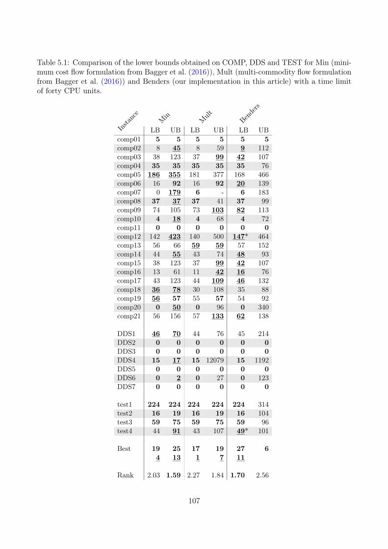
Table 5.1: Comparison of the lower bounds obtained on COMP, DDS and TEST for Min (mini-mum cost flow formulation from Bagger et al. (2016)), Mult (multi-commodity flow formulationfrom Bagger et al. (2016)) and Benders (our implementation in this article) with a time limitof forty CPU units.

Min

Mult

Bende

rs

Insta

nce

LB UB LB UB LB UBcomp01 5 5 5 5 5 5comp02 8 45 8 59 9 112comp03 38 123 37 99 42 107comp04 35 35 35 35 35 76comp05 186 355 181 377 168 466comp06 16 92 16 92 20 139comp07 0 179 6 - 6 183comp08 37 37 37 41 37 99comp09 74 105 73 103 82 113comp10 4 18 4 68 4 72comp11 0 0 0 0 0 0comp12 142 423 140 500 147* 464comp13 56 66 59 59 57 152comp14 44 55 43 74 48 93comp15 38 123 37 99 42 107comp16 13 61 11 42 16 76comp17 43 123 44 109 46 132comp18 36 78 30 108 35 88comp19 56 57 55 57 54 92comp20 0 50 0 96 0 340comp21 56 156 57 133 62 138

DDS1 46 70 44 76 45 214DDS2 0 0 0 0 0 0DDS3 0 0 0 0 0 0DDS4 15 17 15 12079 15 1192DDS5 0 0 0 0 0 0DDS6 0 2 0 27 0 123DDS7 0 0 0 0 0 0

test1 224 224 224 224 224 314test2 16 19 16 19 16 104test3 59 75 59 75 59 96test4 44 91 43 107 49* 101

Best 19 25 17 19 27 64 13 1 7 11

Rank 2.03 1.59 2.27 1.84 1.70 2.56

107

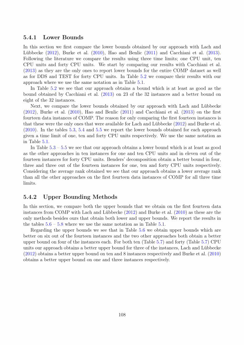
5.4.1 Lower Bounds

In this section we first compare the lower bounds obtained by our approach with Lach andLübbecke (2012), Burke et al. (2010), Hao and Benlic (2011) and Cacchiani et al. (2013).Following the literature we compare the results using three time limits; one CPU unit, tenCPU units and forty CPU units. We start by comparing our results with Cacchiani et al.(2013) as they are the only ones to report lower bounds for the entire COMP dataset as wellas for DDS and TEST for forty CPU units. In Table 5.2 we compare their results with ourapproach where we use the same notation as in Table 5.1.

In Table 5.2 we see that our approach obtains a bound which is at least as good as thebound obtained by Cacchiani et al. (2013) on 23 of the 32 instances and a better bound oneight of the 32 instances.

Next, we compare the lower bounds obtained by our approach with Lach and Lübbecke(2012), Burke et al. (2010), Hao and Benlic (2011) and Cacchiani et al. (2013) on the firstfourteen data instances of COMP. The reason for only comparing the first fourteen instances isthat these were the only ones that were available for Lach and Lübbecke (2012) and Burke et al.(2010). In the tables 5.3, 5.4 and 5.5 we report the lower bounds obtained for each approachgiven a time limit of one, ten and forty CPU units respectively. We use the same notation asin Table 5.1.

In Table 5.3 – 5.5 we see that our approach obtains a lower bound which is at least as goodas the other approaches in ten instances for one and ten CPU units and in eleven out of thefourteen instances for forty CPU units. Benders’ decomposition obtain a better bound in four,three and three out of the fourteen instances for one, ten and forty CPU units respectively.Considering the average rank obtained we see that our approach obtains a lower average rankthan all the other approaches on the first fourteen data instances of COMP for all three timelimits.

5.4.2 Upper Bounding Methods

In this section, we compare both the upper bounds that we obtain on the first fourteen datainstances from COMP with Lach and Lübbecke (2012) and Burke et al. (2010) as these are theonly methods besides ours that obtain both lower and upper bounds. We report the results inthe tables 5.6 – 5.8 where we use the same notation as in Table 5.1.

Regarding the upper bounds we see that in Table 5.6 we obtain upper bounds which arebetter on six out of the fourteen instances and the two other approaches both obtain a betterupper bound on four of the instances each. For both ten (Table 5.7) and forty (Table 5.7) CPUunits our approach obtains a better upper bound for three of the instances, Lach and Lübbecke(2012) obtains a better upper bound on ten and 8 instances respectively and Burke et al. (2010)obtains a better upper bound on one and three instances respectively.

108

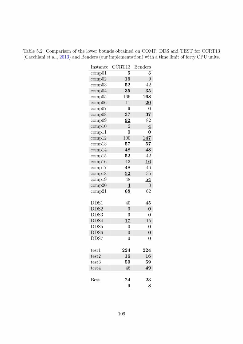
Table 5.2: Comparison of the lower bounds obtained on COMP, DDS and TEST for CCRT13(Cacchiani et al., 2013) and Benders (our implementation) with a time limit of forty CPU units.

Instance CCRT13 Benderscomp01 5 5comp02 16 9comp03 52 42comp04 35 35comp05 166 168comp06 11 20comp07 6 6comp08 37 37comp09 92 82comp10 2 4comp11 0 0comp12 100 147comp13 57 57comp14 48 48comp15 52 42comp16 13 16comp17 48 46comp18 52 35comp19 48 54comp20 4 0comp21 68 62

DDS1 40 45DDS2 0 0DDS3 0 0DDS4 17 15DDS5 0 0DDS6 0 0DDS7 0 0

test1 224 224test2 16 16test3 59 59test4 46 49

Best 24 239 8

109

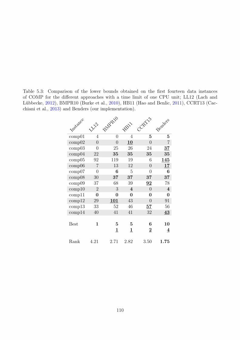
Table 5.3: Comparison of the lower bounds obtained on the first fourteen data instancesof COMP for the different approaches with a time limit of one CPU unit; LL12 (Lach andLübbecke, 2012), BMPR10 (Burke et al., 2010), HB11 (Hao and Benlic, 2011), CCRT13 (Cac-chiani et al., 2013) and Benders (our implementation).

Instance

LL12

BMPR

10

HB11

CCRT13

Benders

comp01 4 0 4 5 5comp02 0 0 10 0 7comp03 0 25 26 24 37comp04 22 35 35 35 35comp05 92 119 19 6 145comp06 7 13 12 0 17comp07 0 6 5 0 6comp08 30 37 37 37 37comp09 37 68 39 92 78comp10 2 3 4 0 4comp11 0 0 0 0 0comp12 29 101 43 0 91comp13 33 52 46 57 56comp14 40 41 41 32 43

Best 1 5 5 6 101 1 2 4

Rank 4.21 2.71 2.82 3.50 1.75

110

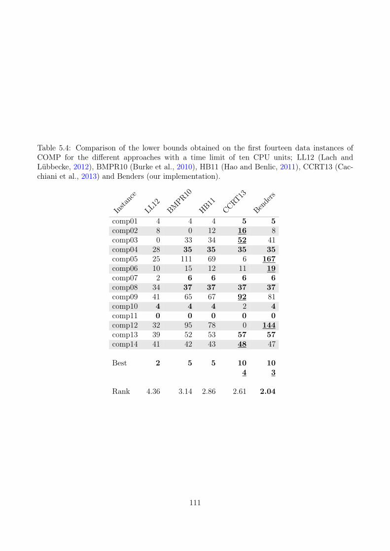
Table 5.4: Comparison of the lower bounds obtained on the first fourteen data instances ofCOMP for the different approaches with a time limit of ten CPU units; LL12 (Lach andLübbecke, 2012), BMPR10 (Burke et al., 2010), HB11 (Hao and Benlic, 2011), CCRT13 (Cac-chiani et al., 2013) and Benders (our implementation).

Instance

LL12

BMPR

10

HB11

CCRT13

Benders

comp01 4 4 4 5 5comp02 8 0 12 16 8comp03 0 33 34 52 41comp04 28 35 35 35 35comp05 25 111 69 6 167comp06 10 15 12 11 19comp07 2 6 6 6 6comp08 34 37 37 37 37comp09 41 65 67 92 81comp10 4 4 4 2 4comp11 0 0 0 0 0comp12 32 95 78 0 144comp13 39 52 53 57 57comp14 41 42 43 48 47

Best 2 5 5 10 104 3

Rank 4.36 3.14 2.86 2.61 2.04

111

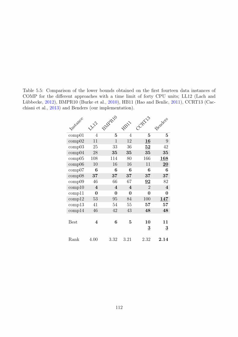
Table 5.5: Comparison of the lower bounds obtained on the first fourteen data instances ofCOMP for the different approaches with a time limit of forty CPU units; LL12 (Lach andLübbecke, 2012), BMPR10 (Burke et al., 2010), HB11 (Hao and Benlic, 2011), CCRT13 (Cac-chiani et al., 2013) and Benders (our implementation).

Instance

LL12

BMPR

10

HB11

CCRT13

Benders

comp01 4 5 4 5 5comp02 11 1 12 16 9comp03 25 33 36 52 42comp04 28 35 35 35 35comp05 108 114 80 166 168comp06 10 16 16 11 20comp07 6 6 6 6 6comp08 37 37 37 37 37comp09 46 66 67 92 82comp10 4 4 4 2 4comp11 0 0 0 0 0comp12 53 95 84 100 147comp13 41 54 55 57 57comp14 46 42 43 48 48

Best 4 6 5 10 113 3

Rank 4.00 3.32 3.21 2.32 2.14

112

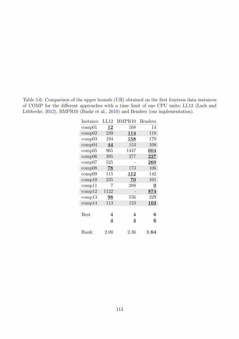
Table 5.6: Comparison of the upper bounds (UB) obtained on the first fourteen data instancesof COMP for the different approaches with a time limit of one CPU units; LL12 (Lach andLübbecke, 2012), BMPR10 (Burke et al., 2010) and Benders (our implementation).

Instance LL12 BMPR10 Benderscomp01 12 168 14comp02 239 114 118comp03 194 158 179comp04 44 153 108comp05 965 1447 604comp06 395 277 227comp07 525 - 260comp08 78 173 106comp09 115 112 142comp10 235 70 101comp11 7 288 0comp12 1122 - 874comp13 98 556 229comp14 113 123 103

Best 4 4 64 4 6

Rank 2.00 2.36 1.64

113

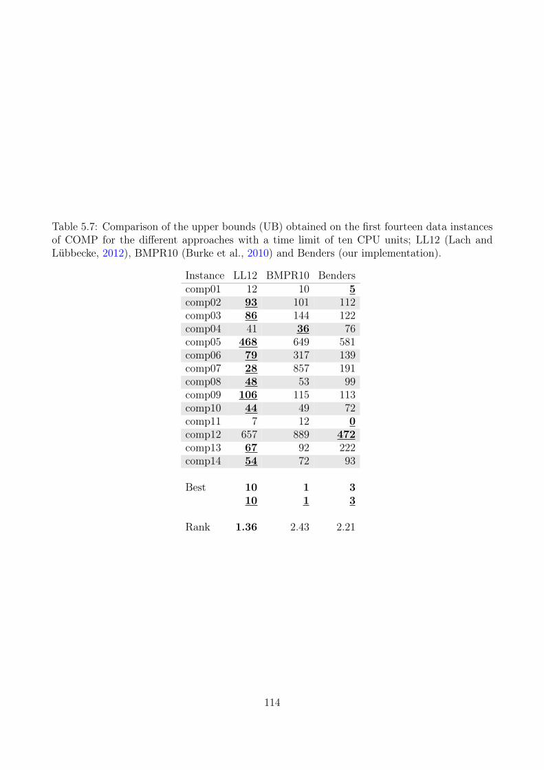
Table 5.7: Comparison of the upper bounds (UB) obtained on the first fourteen data instancesof COMP for the different approaches with a time limit of ten CPU units; LL12 (Lach andLübbecke, 2012), BMPR10 (Burke et al., 2010) and Benders (our implementation).

Instance LL12 BMPR10 Benderscomp01 12 10 5comp02 93 101 112comp03 86 144 122comp04 41 36 76comp05 468 649 581comp06 79 317 139comp07 28 857 191comp08 48 53 99comp09 106 115 113comp10 44 49 72comp11 7 12 0comp12 657 889 472comp13 67 92 222comp14 54 72 93

Best 10 1 310 1 3

Rank 1.36 2.43 2.21

114

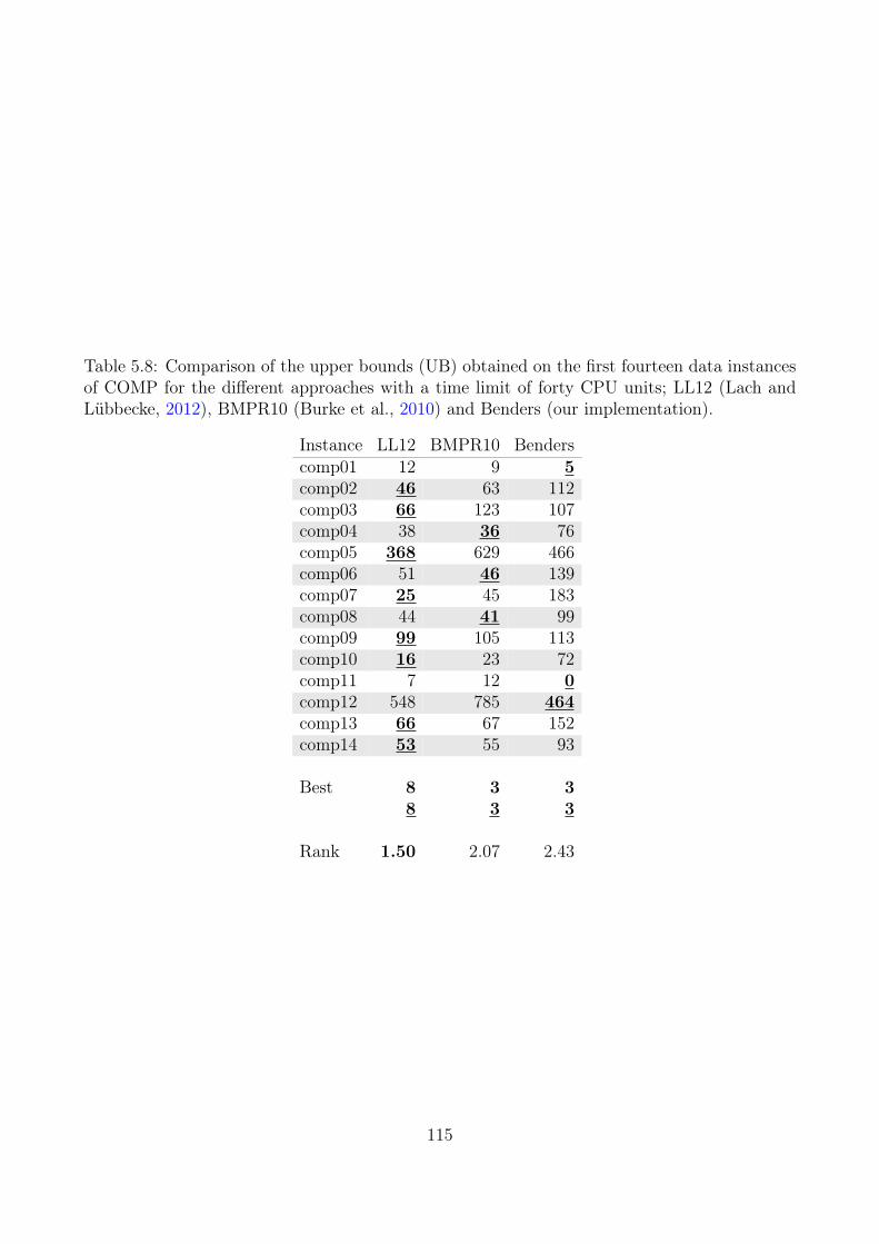
Table 5.8: Comparison of the upper bounds (UB) obtained on the first fourteen data instancesof COMP for the different approaches with a time limit of forty CPU units; LL12 (Lach andLübbecke, 2012), BMPR10 (Burke et al., 2010) and Benders (our implementation).

Instance LL12 BMPR10 Benderscomp01 12 9 5comp02 46 63 112comp03 66 123 107comp04 38 36 76comp05 368 629 466comp06 51 46 139comp07 25 45 183comp08 44 41 99comp09 99 105 113comp10 16 23 72comp11 7 12 0comp12 548 785 464comp13 66 67 152comp14 53 55 93

Best 8 3 38 3 3

Rank 1.50 2.07 2.43

115

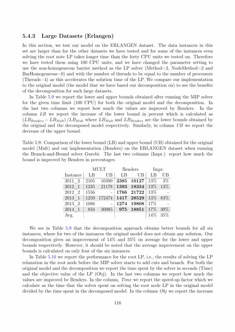
5.4.3 Large Datasets (Erlangen)

In this section, we test our model on the ERLANGEN dataset. The data instances in thisset are larger than for the other datasets we have tested and for some of the instances evensolving the root note LP takes longer time than the forty CPU units we tested on. Thereforewe have tested them using 100 CPU units, and we have changed the parameter setting touse the non-homogeneous barrier method as the LP solver (Method=2, NodeMethod=2 andBarHomogeneous=0) and with the number of threads to be equal to the number of processors(Threads=4) as this accelerates the solution time of the LP. We compare our implementationto the original model (the model that we have based our decomposition on) to see the benefitsof the decomposition for such large datasets.

In Table 5.9 we report the lower and upper bounds obtained after running the MIP solverfor the given time limit (100 CPU) for both the original model and the decomposition. Inthe last two columns we report how much the values are improved by Benders. In thecolumn LB we report the increase of the lower bound in percent which is calculated as(LBBenders − LBMult) /LBMult where LBMult and LBBenders are the lower bounds obtained bythe original and the decomposed model respectively. Similarly, in column UB we report thedecrease of the upper bound.

Table 5.9: Comparison of the lower bound (LB) and upper bound (UB) obtained for the originalmodel (Mult) and our implementation (Benders) on the ERLANGEN dataset when runningthe Branch-and-Bound solver Gurobi. The last two columns (Impr.) report how much thebound is improved by Benders in percentages.

MULT Benders Impr.Instance LB UB LB UB LB UB2011_2 2105 10390 2385 10127 13% 3%2012_1 1235 21178 1393 18334 13% 13%2012_2 1556 - 1766 21722 13% -2013_1 1259 172474 1417 28529 13% 83%2013_2 1086 - 1274 19808 17% -2014_1 834 30985 975 18851 17% 39%Avg. 14% 35%

We see in Table 5.9 that the decomposition approach obtains better bounds for all sixinstances, where for two of the instances the original model does not obtain any solution. Ourdecomposition gives an improvement of 14% and 35% on average for the lower and upperbounds respectively. However, it should be noted that the average improvement on the upperbounds is calculated on only four of the six insrances

In Table 5.10 we report the performance for the root LP, i.e., the results of solving the LPrelaxation in the root node before the MIP solver starts to add cuts and branch. For both theoriginal model and the decomposition we report the time spent by the solver in seconds (Time)and the objective value of the LP (Obj). In the last two columns we report how much thevalues are improved be Benders. In the column, Time we report the speed-up factor which wecalculate as the time that the solver spent on solving the root node LP in the original modeldivided by the time spent in the decomposed model. In the column Obj we report the increase

116

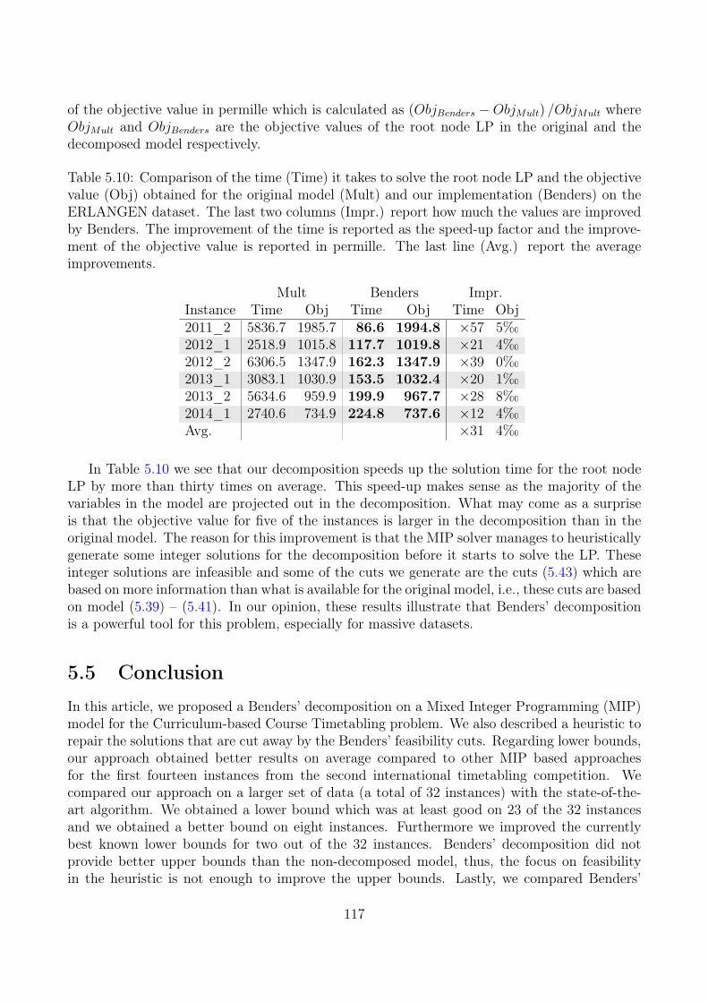
of the objective value in permille which is calculated as (ObjBenders −ObjMult) /ObjMult whereObjMult and ObjBenders are the objective values of the root node LP in the original and thedecomposed model respectively.

Table 5.10: Comparison of the time (Time) it takes to solve the root node LP and the objectivevalue (Obj) obtained for the original model (Mult) and our implementation (Benders) on theERLANGEN dataset. The last two columns (Impr.) report how much the values are improvedby Benders. The improvement of the time is reported as the speed-up factor and the improve-ment of the objective value is reported in permille. The last line (Avg.) report the averageimprovements.

Mult Benders Impr.Instance Time Obj Time Obj Time Obj2011_2 5836.7 1985.7 86.6 1994.8 ×57 5‰2012_1 2518.9 1015.8 117.7 1019.8 ×21 4‰2012_2 6306.5 1347.9 162.3 1347.9 ×39 0‰2013_1 3083.1 1030.9 153.5 1032.4 ×20 1‰2013_2 5634.6 959.9 199.9 967.7 ×28 8‰2014_1 2740.6 734.9 224.8 737.6 ×12 4‰Avg. ×31 4‰

In Table 5.10 we see that our decomposition speeds up the solution time for the root nodeLP by more than thirty times on average. This speed-up makes sense as the majority of thevariables in the model are projected out in the decomposition. What may come as a surpriseis that the objective value for five of the instances is larger in the decomposition than in theoriginal model. The reason for this improvement is that the MIP solver manages to heuristicallygenerate some integer solutions for the decomposition before it starts to solve the LP. Theseinteger solutions are infeasible and some of the cuts we generate are the cuts (5.43) which arebased on more information than what is available for the original model, i.e., these cuts are basedon model (5.39) – (5.41). In our opinion, these results illustrate that Benders’ decompositionis a powerful tool for this problem, especially for massive datasets.

5.5 Conclusion

In this article, we proposed a Benders’ decomposition on a Mixed Integer Programming (MIP)model for the Curriculum-based Course Timetabling problem. We also described a heuristic torepair the solutions that are cut away by the Benders’ feasibility cuts. Regarding lower bounds,our approach obtained better results on average compared to other MIP based approachesfor the first fourteen instances from the second international timetabling competition. Wecompared our approach on a larger set of data (a total of 32 instances) with the state-of-the-art algorithm. We obtained a lower bound which was at least good on 23 of the 32 instancesand we obtained a better bound on eight instances. Furthermore we improved the currentlybest known lower bounds for two out of the 32 instances. Benders’ decomposition did notprovide better upper bounds than the non-decomposed model, thus, the focus on feasibilityin the heuristic is not enough to improve the upper bounds. Lastly, we compared Benders’

117

decomposition to the MIP model that the decomposition originates from on six additional datainstances that are much larger than the other 32 instances. The results showed the benefit ofimplementing Benders’ decomposition as both the lower and upper bounds were better for allthe instances compared to the original model. To our knowledge, no other studies have testedMIP based methods on these data instances, so we improved the best known lower bounds onall six instances.

AcknowledgmentsThe authors would like to thank Assistant Professor Evelien van der Hurk for her valuablefeedback to improve the manuscript.

Funding: This work is part of an industrial PhD project funded by Innovation Fund Den-mark (IFD). IFD has supported this work solely financially and has not taken part in anyresearch related activities.

ReferencesAhuja, R., Magnanti, T., and Orlin, J. (2013). Network Flows: Theory, Algorithms, and Appli-

cations. Always learning. Pearson Education Limited. isbn: 9781292042701. url: https://books.google.ca/books?id=rFuLngEACAAJ.

Bagger, N.-C. F., Simon, K., Sørensen, M., and Stidsen, T. R. (2016). Flow Formulationsfor Curriculum-based Course Timetabling. Available on Optimization Online. url: http://www.optimization-online.org/DB_HTML/2016/12/5786.html.

Benders, J. (1962). “Partitioning procedures for solving mixed-variables programming prob-lems”. English. In: Numerische Mathematik 4.1, pp. 238–252. issn: 0029-599X. doi: 10.1007/BF01386316. url: http://dx.doi.org/10.1007/BF01386316.

Bettinelli, A., Cacchiani, V., Roberti, R., and Toth, P. (2015). “An overview of curriculum-basedcourse timetabling”. In: TOP, pp. 1–37.

Bonutti, A., De Cesco, F., Di Gaspero, L., and Schaerf, A. (2012). “Benchmarking curriculum-based course timetabling: Formulations, data formats, instances, validation, visualization,and results”. In: Annals of Operations Research 194.1, pp. 59–70.

Bonutti, A., Gaspero, L. D., and Schaerf, A. (2016). Curriculum-Based Course TimeTabling.http://tabu.diegm.uniud.it/ctt/index.php[Retrieved 30/12-2016].

Burke, E. K., Mareček, J., Parkes, A. J., and Rudová, H. (2008). “Penalising Patterns in Timeta-bles: Novel Integer Programming Formulations”. In: Operations Research Proceedings 2007.Ed. by J. Kalcsics and S. Nickel. Vol. 2007. Operations Research Proceedings. 10.1007/978-3-540-77903-2_63. Springer Berlin Heidelberg, pp. 409–414. isbn: 978-3-540-77903-2.

Burke, E. K., Mareček, J., Parkes, A. J., and Rudová, H. (2010). “A supernodal formulation ofvertex colouring with applications in course timetabling”. In: Annals of Operations Research179.1, pp. 105–130.

Burke, E. K., Mareček, J., Parkes, A. J., and Rudová, H. (2012). “A branch-and-cut proce-dure for the Udine Course Timetabling problem”. In: Annals of Operations Research 194.1,pp. 71–87.

118

Cacchiani, V., Caprara, A., Roberti, R., and Toth, P. (2013). “A new lower bound for curriculum-based course timetabling”. In: Computers and Operation Research 40.10, pp. 2466–2477. doi:10.1016/j.cor.2013.02.010.

Di Gaspero, L., McCollum, B., and Schaerf, A. (2007). The Second International TimetablingCompetition (ITC-2007): Curriculum-based Course Timetabling (Track 3). Tech. rep. Schoolof Electronics, Electrical Engineering and Computer Science, Queenes University SARCBuilding, Belfast, United Kingdom.

Di Gaspero, L. and Schaerf, A. (2003). “Multi-neighbourhood Local Search with Applicationto Course Timetabling”. English. In: Practice and Theory of Automated Timetabling IV.Ed. by E. Burke and P. De Causmaecker. Vol. 2740. Lecture Notes in Computer Science.Springer Berlin Heidelberg, pp. 262–275. isbn: 978-3-540-40699-0. doi: 10.1007/978-3-540-45157-0_17. url: http://dx.doi.org/10.1007/978-3-540-45157-0_17.

Fischetti, M. (2015). The simpler the better: Thinning out MIP’s by Occam’s razor. Presen-tation at CORS/INFORMS 2015 Joint International Meeting in Montréal. Slides retrievedDecember 16, 2016, from: http://www.dei.unipd.it/~fisch/papers/slides/2015%20CORS%20%5bFischetti%20-%20Occam%20Razor%5d.pdf.

Geoffrion, A. M. (1972). “Generalized benders decomposition”. In: Journal of optimization the-ory and applications 10.4, pp. 237–260.

Gurobi Optimization Inc. (2015). Gurobi Optimizer Reference Manual. url: http://www.gurobi.com.

Hao, J. K. and Benlic, U. (2011). “Lower bounds for the ITC-2007 curriculum-based coursetimetabling problem”. In: European Journal of Operational Research 212.3, pp. 464–472.

Lach, G. and Lübbecke, M. (2012). “Curriculum based course timetabling: new solutions toUdine benchmark instances”. In: Annals of Operations Research 194, pp. 255–272. issn:0254-5330.

Lach, G. and Lübbecke, M. E. (2008). “Optimal University Course Timetables and the Par-tial Transversal Polytope”. In: International Workshop on Experimental and Efficient Algo-rithms. Springer, pp. 235–248.

Lübbecke, M. E. (2015). “Comments on: An overview of curriculum-based course timetabling”.In: TOP 23.2, pp. 359–361.

Martin, R. K. (1999). Large scale linear and integer optimization: a unified approach. KluwerAcademic Publishers.

McCollum, B., Schaerf, A., Paechter, B., McMullan, P., Lewis, R., Parkes, A. J., Gaspero, L. D.,Qu, R., and Burke, E. K. (2010). “Setting the Research Agenda in Automated Timetabling:The Second International Timetabling Competition”. In: INFORMS Journal on Computing22.1, pp. 120–130.

119

Part III

Lower Bounding Methods

121

6 Daily Course Pattern Formulation andValid Inequalities for theCurriculum-based Course TimetablingProblem

Niels-Christian F. Baggera,b · Guy Desaulniersc,d · Jacques Desrosierse

amORetime research group, Management Science, Department of Management Engineering,Technical University of Denmark, Produktionstorvet, Building 426B, DK-2800 Kgs. Lyngby,Denmark, http://www.moretime.man.dtu.dk/

bMaCom A/S, Vesterbrogade 48, 1., DK-1620 København V, DenmarkcGERAD – HEC Montréal 3000, Côte-Sainte-Catherine, Montréal, Canada H3T 2A7dPolytechnique Montréal, Montréal, Canada H3C 3A7eHEC Montréal, Montréal, Canada H3T 2A7

Status: Submitted to Journal of Scheduling

Abstract: In this paper, we propose an integer programming model for obtaininglower bounds for the curriculum-based course timetabling problem, in which weeklyassignments for courses into rooms and periods are considered. The model is apattern formulation where a pattern is an assignment of a course into a set ofperiods on one day. Different preprocessing techniques are implemented to reducethe number of variables and valid inequalities are derived and added to the model.The proposed model is tested on 21 real-world data instances. On 17 of theseinstances the best know solutions have been proven optimal and for the remainingfour our model improves the lower bounds for three of them.

Keywords: Course Timetabling · Integer Programming · Preprocessing · ValidInequalities

123

6.1 IntroductionThe problem considered in this paper is the Curriculum-based Course Timetabling Problem(CCT) as described by Di Gaspero et al. (2007). The interest in this problem has increasedas it was used as one of three problems for the Second International Timetabling Competition(ITC2007) in 2007 (Di Gaspero et al., 2007; McCollum et al., 2010). In connection to ITC2007,a website was developed (Bonutti et al., 2016) where it is possible for researchers to uploadsolutions and to report refined lower bounds. Twenty-one data sets were provided for the com-petition based on real world instances. Seven of these were hidden until after the competition.For the 21 data sets, most of them has been closed, meaning that the best solutions found havebeen proven optimal. However there are still four open data sets left and the aim of this paperis to reduce the gaps by improving the lower bounds.

6.1.1 Problem Description

A set of courses is given, each having a predetermined number of lectures to be scheduled.Each course is taught be exactly one lecturer. A set of curricula is also given, each consistingof a set of courses. A course can belong to several curricula. Furthermore a time horizon interms of a number of days that all the lectures need to be scheduled in is given. Each day isdivided into a number of uniform time slots and a day and time slot pair is referred to as aperiod. It is assumed that each lecture takes up exactly one period. Besides scheduling thelectures into periods, it is also needed to choose a room for the lecture to take place in. Finallysome constraints are also given. These can either be hard or soft. Any feasible timetableshould fulfil all the hard constraints, i.e., a timetable is considered feasible if and only if allthe hard-constraints have no violations. The objective is then to find a feasible timetable whileminimizing a weighted sum of the violation of the soft constraints.

The problem formulated by Di Gaspero et al. (2007) contains four hard constraints as listedbelow:

Availability (A): A course can have specific periods defined as unavailable periods. Everylecture scheduled in such a period is considered as one violation.

Conflicts (C): A pair of lectures is considered as conflicting if they belong to the same cur-riculum or are taught by the same lecturer. If a conflicting pair of lectures is scheduledin the same period, this is considered as one violation.

Lectures (L): Each course has a predetermined number of lectures to be scheduled in differentperiods. If a lecture is not scheduled or if two lectures of a course are scheduled in thesame period, this is counted as one violation.

Room Occupancy (RO): For every room and every period, at most one lecture should bescheduled. For every room and period, every additional lecture is considered as oneviolation.

In our approach, we are only focusing on scheduling the courses into the periods. The onlyhard constraint involving the rooms is RO and this constraint can still be fulfilled since it ispossible to put any course into any room. Therefore we just have to ensure that we do not

124

schedule more courses into a single period than the number of available rooms in the datainstance. The problem also contains four soft constraints for which we minimize the number ofviolations. These are listed below:

Isolated Lectures (IL): It is desired to create compact schedules. A lecture is isolated ifno other lectures are scheduled for a curriculum on the same day in either a directlypreceding or successive time slot (i.e., in consecutive time slots). Each isolated lecture iscounted as one violation.

Example 6.1. Consider a curriculum containingcourses C001 and C002, a day with six time slots, and the following schedules on thatday:

C001: R001

C002: R002

The schedules shows that course C001 has a lecture in the second time slot while C002 hasa lecture in the fourth time slot. Since these time slots are not adjacent, this means thatthe schedules count two violations on that day. Consider now the following schedules:

C001: R001

C002: R002

Course C001 has a lecture in the fourth time slot while C002 has a lecture in the thirdone. These time slots are adjacent and these schedules do not count any violations onthat day.

Minimum Working Days (MWD): For each course, a day is defined as a working day if atleast one lecture is scheduled on it. For each course, a minimum number of working daysis requested and each day below this minimum counts as one violation.

Room Capacity (RC): There is a number of students attending a given course and eachroom has a specific capacity. If the number of students assigned is greater than the roomcapacity, then every student that cannot be accommodated counts as one violation.

Room Stability (RStab): For every course, it is desired to schedule all lectures in just oneroom. Every additional room is counted as one violation.

As mentioned before, we only consider the scheduling of the courses into periods and ignorethe assignment of rooms. Therefore we can only take the soft constraints IL and MWD intoaccount which means that our approach is a relaxation of the original problem. Hence anyvalid lower bounds for our model are also valid lower bounds for the original problem.

It should be noted that the constraint IL is usually referred to as curriculum compactnessin the literature. We have chosen to name it isolated lectures as multiple ways of formulatingcurriculum compactness are described in Bonutti et al. (2012) and this is the name they givefor this formulation.

125

6.1.2 Related Work

As our focus is on lower bounds, we focus on the literature that have reported lower bounds aswell. For the interested reader, we refer to Bettinelli et al. (2015) as they give more detaileddescriptions of all the methods presented here as well as descriptions of many more methodsincluding those to obtain upper bounds.

Burke et al. (2008), Burke et al. (2010), and Burke et al. (2012) describes a compact IntegerLinear Programming (ILP) formulation which can be solved by a commercial ILP solver. Theydiscover that this formulation is very hard to solve and tackle this in various ways. In Burkeet al. (2010), one way to get a lower bound is to consider a relaxed version of the problem bysetting the weights of the two room-related constraints RC and RStab to zero. This allowsthem to only consider the time-scheduling part of the problem. Furthermore a constraint isadded to ensure that no more courses are scheduled in any time period than the total numberof rooms available. Note that this is the same relaxation of the original problem that we areconsidering. They note that the before mentioned approach can be thought of as aggregatingall the rooms into a single multi-room, where the capacity of this room is equal to the largestroom. Another approach is to divide the rooms into sets of multi-rooms. For each multi-room,the capacity is equal to the largest room in the set and the maximum number of lectures thatcan take place in a multi-room in any period is equal to the number of rooms in the set. Thisallows them to partially include the room related soft constraints. After finding a solution toone of the before mentioned relaxations, the rooms are included in the model again and thesolution obtained from the relaxation is used to guide the search by either fixing the periodsthat the lectures are assigned to or by fixing the days. In Burke et al. (2008), they enumerateall patterns for each day and for each curriculum and add the costs of these patterns as cuts.These cuts are also used in Burke et al. (2012) where they develop a cutting plane procedureand the cuts from Burke et al. (2008) are added dynamically as they are violated. Furthermoreother cuts are derived including clique cuts and some more problem specific cuts. The reportedresults show that the cutting plane approach leads to better performances compared to thecompact ILP formulation.

In Lach and Lübbecke (2012), the problem is decomposed into two stages: the first findsa feasible time-schedule, the second assigns the rooms to the lectures. This is based on theirwork in Lach and Lübbecke (2008) where they considered only hard constraints and showedthat specific cuts could be added to the first stage problem to ensure feasible solutions. InLach and Lübbecke (2012), they show how the RC constraint can be included in the first stageproblem leaving only the RStab constraint for the second stage.

In Hao and Benlic (2011), the focus is on obtaining lower bounds for the first stage problemfrom Lach and Lübbecke (2012). Their approach is to decompose the courses and compute lowerbounds for each of the decomposed sets of courses. A lower bound for the original problem isthen calculated as the sum of the lower bounds of the decomposed sets of courses. The selectionof the decomposition is embedded in a Tabu Search procedure (see Glover and Laguna, 2013).

Asín Achá and Nieuwenhuis (2012) encodes the constraints as satisfiability clauses. Theyapply different encodings both treating all constraints as hard and relaxing some or all of thesoft constraints. They are able to prove optimality of more than half of the ITC2007 data sets.

Finally, Cacchiani et al. (2013) consider a model based on column generation. The idea is tosplit up the problem into two subproblems. One subproblem focuses on the room related softconstraints RC and RO. The other subproblem focuses on the time related soft constraints

126

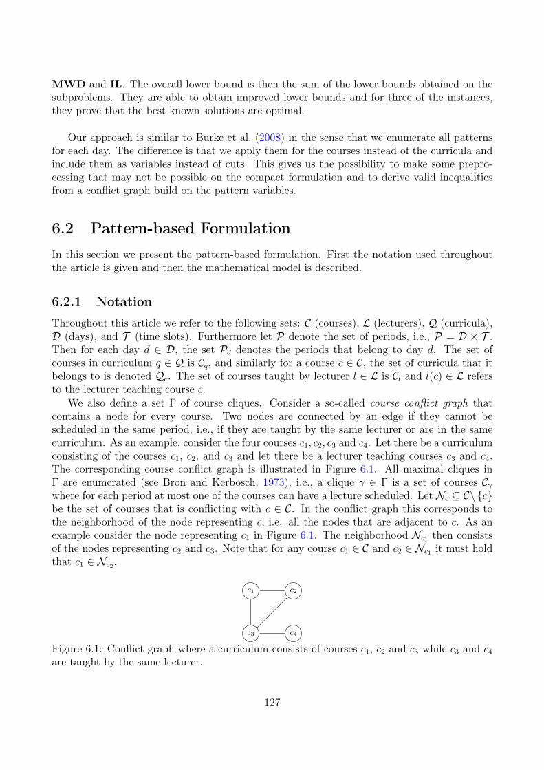
MWD and IL. The overall lower bound is then the sum of the lower bounds obtained on thesubproblems. They are able to obtain improved lower bounds and for three of the instances,they prove that the best known solutions are optimal.

Our approach is similar to Burke et al. (2008) in the sense that we enumerate all patternsfor each day. The difference is that we apply them for the courses instead of the curricula andinclude them as variables instead of cuts. This gives us the possibility to make some prepro-cessing that may not be possible on the compact formulation and to derive valid inequalitiesfrom a conflict graph build on the pattern variables.

6.2 Pattern-based Formulation

In this section we present the pattern-based formulation. First the notation used throughoutthe article is given and then the mathematical model is described.

6.2.1 Notation

Throughout this article we refer to the following sets: C (courses), L (lecturers), Q (curricula),D (days), and T (time slots). Furthermore let P denote the set of periods, i.e., P = D × T .Then for each day d ∈ D, the set Pd denotes the periods that belong to day d. The set ofcourses in curriculum q ∈ Q is Cq, and similarly for a course c ∈ C, the set of curricula that itbelongs to is denoted Qc. The set of courses taught by lecturer l ∈ L is Cl and l(c) ∈ L refersto the lecturer teaching course c.

We also define a set Γ of course cliques. Consider a so-called course conflict graph thatcontains a node for every course. Two nodes are connected by an edge if they cannot bescheduled in the same period, i.e., if they are taught by the same lecturer or are in the samecurriculum. As an example, consider the four courses c1, c2, c3 and c4. Let there be a curriculumconsisting of the courses c1, c2, and c3 and let there be a lecturer teaching courses c3 and c4.The corresponding course conflict graph is illustrated in Figure 6.1. All maximal cliques inΓ are enumerated (see Bron and Kerbosch, 1973), i.e., a clique γ ∈ Γ is a set of courses Cγwhere for each period at most one of the courses can have a lecture scheduled. Let Nc ⊆ C\ {c}be the set of courses that is conflicting with c ∈ C. In the conflict graph this corresponds tothe neighborhood of the node representing c, i.e. all the nodes that are adjacent to c. As anexample consider the node representing c1 in Figure 6.1. The neighborhood Nc1 then consistsof the nodes representing c2 and c3. Note that for any course c1 ∈ C and c2 ∈ Nc1 it must holdthat c1 ∈ Nc2 .

c1 c2

c3 c4

Figure 6.1: Conflict graph where a curriculum consists of courses c1, c2 and c3 while c3 and c4

are taught by the same lecturer.

127

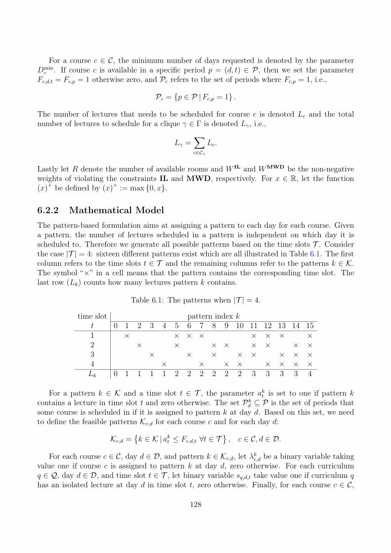
For a course c ∈ C, the minimum number of days requested is denoted by the parameterDminc . If course c is available in a specific period p = (d, t) ∈ P , then we set the parameter

Fc,d,t = Fc,p = 1 otherwise zero, and Pc refers to the set of periods where Fc,p = 1, i.e.,

Pc = {p ∈ P |Fc,p = 1} .

The number of lectures that needs to be scheduled for course c is denoted Lc and the totalnumber of lectures to schedule for a clique γ ∈ Γ is denoted Lγ, i.e.,

Lγ =∑c∈Cγ

Lc.

Lastly let R denote the number of available rooms and W IL and WMWD be the non-negativeweights of violating the constraints IL and MWD, respectively. For x ∈ R, let the function(x)+ be defined by (x)+ := max {0, x}.

6.2.2 Mathematical Model

The pattern-based formulation aims at assigning a pattern to each day for each course. Givena pattern, the number of lectures scheduled in a pattern is independent on which day it isscheduled to. Therefore we generate all possible patterns based on the time slots T . Considerthe case |T | = 4: sixteen different patterns exist which are all illustrated in Table 6.1. The firstcolumn refers to the time slots t ∈ T and the remaining columns refer to the patterns k ∈ K.The symbol “×” in a cell means that the pattern contains the corresponding time slot. Thelast row (Lk) counts how many lectures pattern k contains.

Table 6.1: The patterns when |T | = 4.

time slot pattern index kt 0 1 2 3 4 5 6 7 8 9 10 11 12 13 14 151 × × × × × × × ×2 × × × × × × × ×3 × × × × × × × ×4 × × × × × × × ×Lk 0 1 1 1 1 2 2 2 2 2 2 3 3 3 3 4

For a pattern k ∈ K and a time slot t ∈ T , the parameter akt is set to one if pattern kcontains a lecture in time slot t and zero otherwise. The set Pkd ⊆ P is the set of periods thatsome course is scheduled in if it is assigned to pattern k at day d. Based on this set, we needto define the feasible patterns Kc,d for each course c and for each day d:

Kc,d ={k ∈ K | akt ≤ Fc,d,t ∀t ∈ T

}, c ∈ C, d ∈ D.

For each course c ∈ C, day d ∈ D, and pattern k ∈ Kc,d, let λkc,d be a binary variable takingvalue one if course c is assigned to pattern k at day d, zero otherwise. For each curriculumq ∈ Q, day d ∈ D, and time slot t ∈ T , let binary variable sq,d,t take value one if curriculum qhas an isolated lecture at day d in time slot t, zero otherwise. Finally, for each course c ∈ C,

128

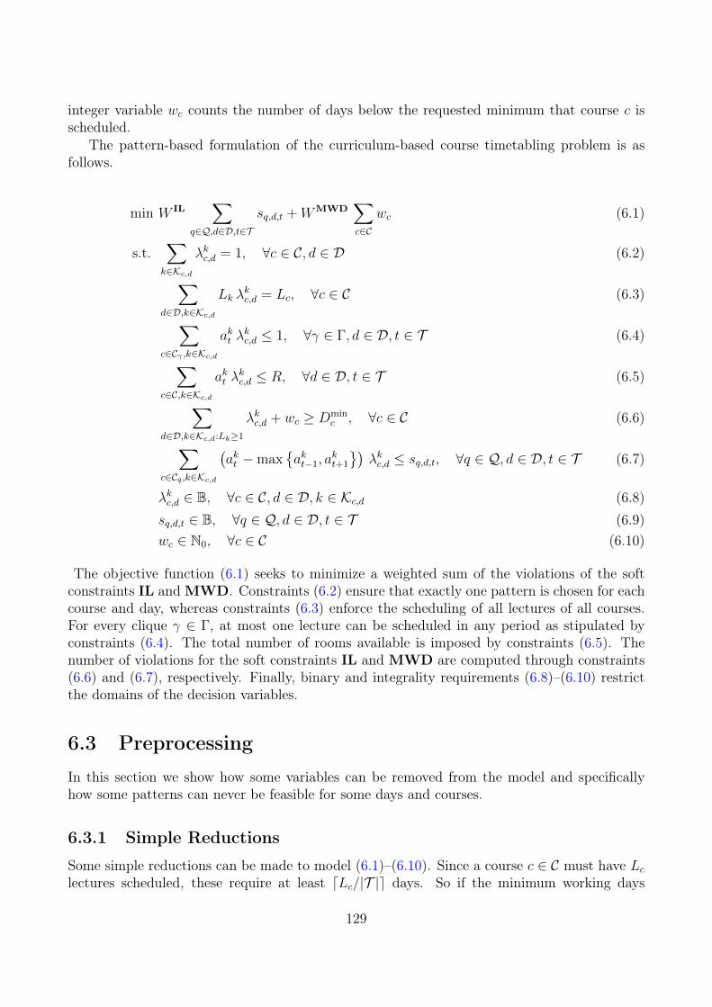
integer variable wc counts the number of days below the requested minimum that course c isscheduled.

The pattern-based formulation of the curriculum-based course timetabling problem is asfollows.

min W IL∑

q∈Q,d∈D,t∈T

sq,d,t +WMWD∑c∈C

wc (6.1)

s.t.∑k∈Kc,d

λkc,d = 1, ∀c ∈ C, d ∈ D (6.2)

∑d∈D,k∈Kc,d

Lk λkc,d = Lc, ∀c ∈ C (6.3)

∑c∈Cγ ,k∈Kc,d

akt λkc,d ≤ 1, ∀γ ∈ Γ, d ∈ D, t ∈ T (6.4)

∑c∈C,k∈Kc,d

akt λkc,d ≤ R, ∀d ∈ D, t ∈ T (6.5)

∑d∈D,k∈Kc,d:Lk≥1

λkc,d + wc ≥ Dminc , ∀c ∈ C (6.6)

∑c∈Cq ,k∈Kc,d

(akt −max

{akt−1, a

kt+1

})λkc,d ≤ sq,d,t, ∀q ∈ Q, d ∈ D, t ∈ T (6.7)

λkc,d ∈ B, ∀c ∈ C, d ∈ D, k ∈ Kc,d (6.8)sq,d,t ∈ B, ∀q ∈ Q, d ∈ D, t ∈ T (6.9)wc ∈ N0, ∀c ∈ C (6.10)

The objective function (6.1) seeks to minimize a weighted sum of the violations of the softconstraints IL and MWD. Constraints (6.2) ensure that exactly one pattern is chosen for eachcourse and day, whereas constraints (6.3) enforce the scheduling of all lectures of all courses.For every clique γ ∈ Γ, at most one lecture can be scheduled in any period as stipulated byconstraints (6.4). The total number of rooms available is imposed by constraints (6.5). Thenumber of violations for the soft constraints IL and MWD are computed through constraints(6.6) and (6.7), respectively. Finally, binary and integrality requirements (6.8)–(6.10) restrictthe domains of the decision variables.

6.3 Preprocessing

In this section we show how some variables can be removed from the model and specificallyhow some patterns can never be feasible for some days and courses.

6.3.1 Simple Reductions

Some simple reductions can be made to model (6.1)–(6.10). Since a course c ∈ C must have Lclectures scheduled, these require at least dLc/|T |e days. So if the minimum working days

129

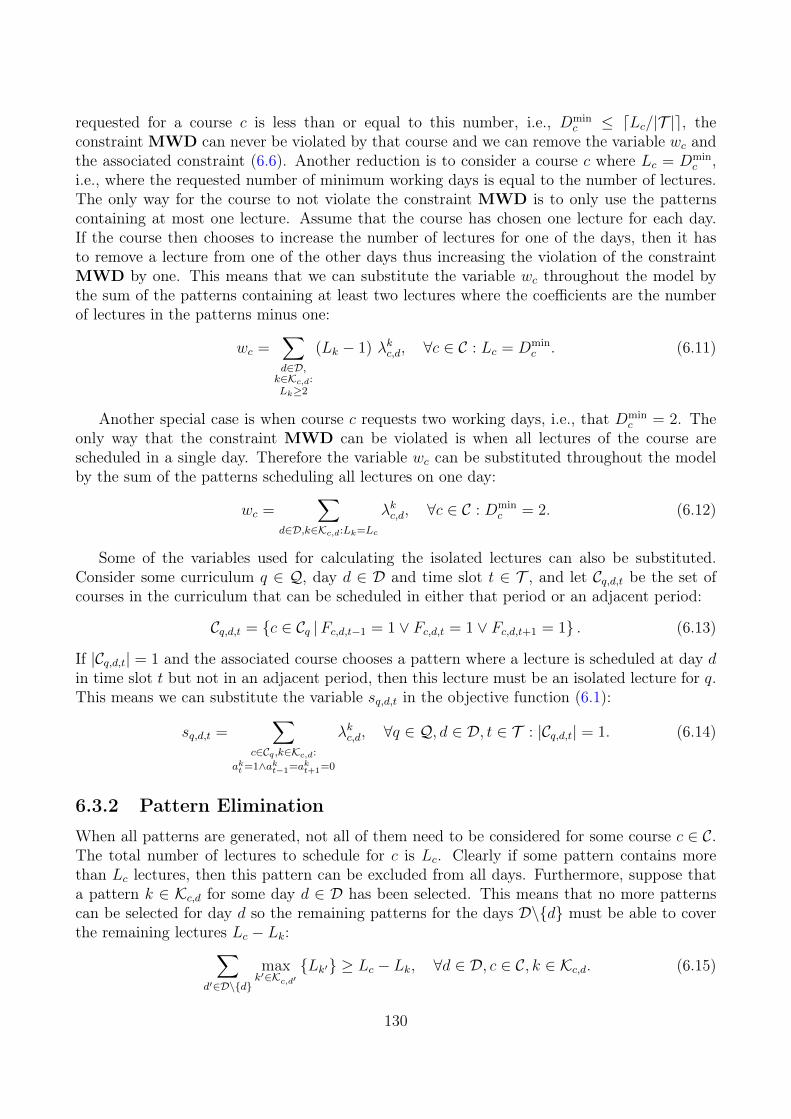
requested for a course c is less than or equal to this number, i.e., Dminc ≤ dLc/|T |e, the

constraint MWD can never be violated by that course and we can remove the variable wc andthe associated constraint (6.6). Another reduction is to consider a course c where Lc = Dmin

c ,i.e., where the requested number of minimum working days is equal to the number of lectures.The only way for the course to not violate the constraint MWD is to only use the patternscontaining at most one lecture. Assume that the course has chosen one lecture for each day.If the course then chooses to increase the number of lectures for one of the days, then it hasto remove a lecture from one of the other days thus increasing the violation of the constraintMWD by one. This means that we can substitute the variable wc throughout the model bythe sum of the patterns containing at least two lectures where the coefficients are the numberof lectures in the patterns minus one:

wc =∑d∈D,k∈Kc,d:Lk≥2

(Lk − 1) λkc,d, ∀c ∈ C : Lc = Dminc . (6.11)

Another special case is when course c requests two working days, i.e., that Dminc = 2. The

only way that the constraint MWD can be violated is when all lectures of the course arescheduled in a single day. Therefore the variable wc can be substituted throughout the modelby the sum of the patterns scheduling all lectures on one day:

wc =∑

d∈D,k∈Kc,d:Lk=Lc

λkc,d, ∀c ∈ C : Dminc = 2. (6.12)

Some of the variables used for calculating the isolated lectures can also be substituted.Consider some curriculum q ∈ Q, day d ∈ D and time slot t ∈ T , and let Cq,d,t be the set ofcourses in the curriculum that can be scheduled in either that period or an adjacent period:

Cq,d,t = {c ∈ Cq |Fc,d,t−1 = 1 ∨ Fc,d,t = 1 ∨ Fc,d,t+1 = 1} . (6.13)

If |Cq,d,t| = 1 and the associated course chooses a pattern where a lecture is scheduled at day din time slot t but not in an adjacent period, then this lecture must be an isolated lecture for q.This means we can substitute the variable sq,d,t in the objective function (6.1):

sq,d,t =∑

c∈Cq ,k∈Kc,d:

akt=1∧akt−1=akt+1=0

λkc,d, ∀q ∈ Q, d ∈ D, t ∈ T : |Cq,d,t| = 1. (6.14)

6.3.2 Pattern Elimination

When all patterns are generated, not all of them need to be considered for some course c ∈ C.The total number of lectures to schedule for c is Lc. Clearly if some pattern contains morethan Lc lectures, then this pattern can be excluded from all days. Furthermore, suppose thata pattern k ∈ Kc,d for some day d ∈ D has been selected. This means that no more patternscan be selected for day d so the remaining patterns for the days D\{d} must be able to coverthe remaining lectures Lc − Lk:∑

d′∈D\{d}

maxk′∈Kc,d′

{Lk′} ≥ Lc − Lk, ∀d ∈ D, c ∈ C, k ∈ Kc,d. (6.15)

130

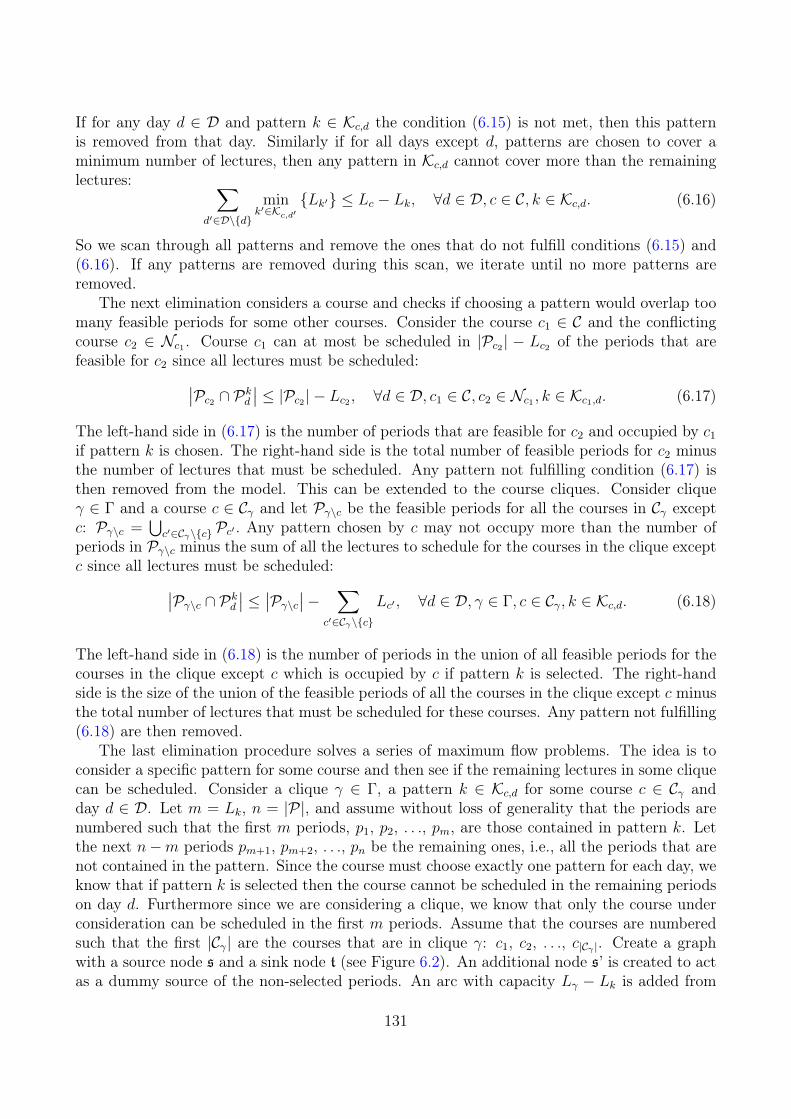
If for any day d ∈ D and pattern k ∈ Kc,d the condition (6.15) is not met, then this patternis removed from that day. Similarly if for all days except d, patterns are chosen to cover aminimum number of lectures, then any pattern in Kc,d cannot cover more than the remaininglectures: ∑

d′∈D\{d}

mink′∈Kc,d′

{Lk′} ≤ Lc − Lk, ∀d ∈ D, c ∈ C, k ∈ Kc,d. (6.16)

So we scan through all patterns and remove the ones that do not fulfill conditions (6.15) and(6.16). If any patterns are removed during this scan, we iterate until no more patterns areremoved.

The next elimination considers a course and checks if choosing a pattern would overlap toomany feasible periods for some other courses. Consider the course c1 ∈ C and the conflictingcourse c2 ∈ Nc1 . Course c1 can at most be scheduled in |Pc2 | − Lc2 of the periods that arefeasible for c2 since all lectures must be scheduled:∣∣Pc2 ∩ Pkd ∣∣ ≤ |Pc2| − Lc2 , ∀d ∈ D, c1 ∈ C, c2 ∈ Nc1 , k ∈ Kc1,d. (6.17)

The left-hand side in (6.17) is the number of periods that are feasible for c2 and occupied by c1

if pattern k is chosen. The right-hand side is the total number of feasible periods for c2 minusthe number of lectures that must be scheduled. Any pattern not fulfilling condition (6.17) isthen removed from the model. This can be extended to the course cliques. Consider cliqueγ ∈ Γ and a course c ∈ Cγ and let Pγ\c be the feasible periods for all the courses in Cγ exceptc: Pγ\c =

⋃c′∈Cγ\{c}Pc′ . Any pattern chosen by c may not occupy more than the number of

periods in Pγ\c minus the sum of all the lectures to schedule for the courses in the clique exceptc since all lectures must be scheduled:∣∣Pγ\c ∩ Pkd ∣∣ ≤ ∣∣Pγ\c∣∣− ∑

c′∈Cγ\{c}

Lc′ , ∀d ∈ D, γ ∈ Γ, c ∈ Cγ, k ∈ Kc,d. (6.18)

The left-hand side in (6.18) is the number of periods in the union of all feasible periods for thecourses in the clique except c which is occupied by c if pattern k is selected. The right-handside is the size of the union of the feasible periods of all the courses in the clique except c minusthe total number of lectures that must be scheduled for these courses. Any pattern not fulfilling(6.18) are then removed.

The last elimination procedure solves a series of maximum flow problems. The idea is toconsider a specific pattern for some course and then see if the remaining lectures in some cliquecan be scheduled. Consider a clique γ ∈ Γ, a pattern k ∈ Kc,d for some course c ∈ Cγ andday d ∈ D. Let m = Lk, n = |P|, and assume without loss of generality that the periods arenumbered such that the first m periods, p1, p2, . . ., pm, are those contained in pattern k. Letthe next n−m periods pm+1, pm+2, . . ., pn be the remaining ones, i.e., all the periods that arenot contained in the pattern. Since the course must choose exactly one pattern for each day, weknow that if pattern k is selected then the course cannot be scheduled in the remaining periodson day d. Furthermore since we are considering a clique, we know that only the course underconsideration can be scheduled in the first m periods. Assume that the courses are numberedsuch that the first |Cγ| are the courses that are in clique γ: c1, c2, . . ., c|Cγ |. Create a graphwith a source node s and a sink node t (see Figure 6.2). An additional node s’ is created to actas a dummy source of the non-selected periods. An arc with capacity Lγ − Lk is added from

131

the source s to the dummy source s’ to model that the first Lk lectures must be scheduled bythe source and the remaining Lγ − Lk lectures must be scheduled by the dummy source. Foreach period p1, p2, . . ., pn, create a node and add an ingoing arc from the source s if the periodis in the set {p1, p2, . . . , pm} and add an ingoing arc from the dummy source s’ if the period isin the set {pm+1, pm+2, . . . , pn}. The capacities of all these arcs are set to one. For each coursec′ ∈

{c1, c2, . . . , c|Qγ |

}, add a node to the graph and add an outgoing arc to the sink t with a

capacity of Lc′ . For each node p ∈ {p1, p2, . . . , pn} and each node c′ ∈{c1, c2, . . . , c|Cγ |

}, add an

arc from p to c′ with capacity a (c′, p) which is set depending on c and k:

a (c′, p) =

Fc′,p if p ∈ {p1, . . . , pm}and c′ = c

Fc′,p if p ∈ {pm+1, . . . , pn}and (c′ 6= c ∨ p /∈ Pd)

0 otherwise.

(6.19)

If p is one of the first m periods, the capacity is set to Fc′,p if c′ = c; if p is one of the n −mlast periods, the capacity is set to Fc′,p if p does not belong to day d or if c′ 6= c. A maximumflow problem is solved and if the total amount of flow is less than the total number of lecturesthat need to be scheduled for the clique, then pattern k can never be feasible for course c atday d, and can thus be removed from Kc,d.

s pm

...

p2

p1

pm+1

...

pn

s’

c2

c1

...

c|Cγ |

t

Lγ −

Lk

1

1

1

1

1

Lc1

Lc2

Lc |C γ|

Figure 6.2: Given a clique γ, maximum flow graph to verify if pattern k for course c ∈ Cγ andday d can be discarded.

132

6.4 Valid Inequalities

In this section some strengthened bounds and valid inequalities are presented.

6.4.1 Implied Bounds

Burke et al. (2012) noted that since all lectures must be scheduled, then at least one day mustbe used by each course c ∈ C meaning that the constraint MWD can at most be violated byDminc − 1. This can be strengthened a bit by noting that at most |T | lectures can be scheduled

every day and so course c must be scheduled in at least dLc/|T |e days:

0 ≤ wc ≤(Dminc −

⌈Lc|T |

⌉)+

, ∀c ∈ C. (6.20)

By considering the constraint A, this can be slightly improved. Let Dc ={d1, d2, . . . , d|D|

}be the days for course c which are sorted such that

∑t∈T Fc,di,t ≥

∑t∈T Fc,dj ,t for every i, j ∈

{1, 2, . . . , |D|} where i < j. Then the minimum number of days that course c will be scheduledis the smallest index i ∈ {1, 2, . . . , |D|} such that the total amount of feasible periods in thedays d1, d2, . . . , di is enough to schedule all lectures of the course. We can then calculate anupper bound on the violation of the constraint MWD:

wuc = Dminc − min

i∈{1,...,|D|}

i∣∣∣∣∣∣∣∣∣∑

j∈{1,...,i},p∈Pdj

Fc,p ≥ Lc

, ∀c ∈ C. (6.21)

It is also possible to calculate the maximum number of days course c can be scheduled in.Obviously it is not possible to schedule more than Lc days. Using the constraint A, it is notpossible to schedule more days than the set of days where at least one of the time slots isfeasible for the course. So a lower bound on the violation of the constraint MWD can also becalculated:

wlc = Dminc −max

{Lc,

∣∣∣∣∣{d ∈ D

∣∣ ∑p∈Pd

Fc,p ≥ 1

}∣∣∣∣∣}, ∀c ∈ C. (6.22)

This gives the following bounds:(wlc)+ ≤ wc ≤ (wuc )+ , ∀c ∈ C. (6.23)

Furthermore since we have just found the minimum and maximum number of days that a coursecan have scheduled lectures, we can add the following inequalities to model (6.1)–(6.10):

∑d∈D,k∈Kc,d:Lk≥1

λkc,d ≥ mini∈{1,...,|D|}

i∣∣∣∣∣∣∣∣∣∑

j∈{1,...,i},p∈Pdj

Fc,p ≥ Lc

, ∀c ∈ C. (6.24)

133

∑d∈D,k∈Kc,d:Lk≥1

λkc,d ≤ max

{Lc,

∣∣∣∣∣{d ∈ D |

∑p∈Pd

Fc,p ≥ 1

}∣∣∣∣∣}, ∀c ∈ C. (6.25)

6.4.2 Extended Cover Inequalities

Consider clique γ ∈ Γ. Since we must schedule the lectures for all courses, trivially the followingmust hold: ∑

c∈Cγ ,d∈D,k∈Kc,d

Lk λkc,d ≤ Lγ, ∀γ ∈ Γ. (6.26)

Note that the conditions (6.26) are knapsack constraints. This means that we can apply knownvalid inequalities such as cover inequalities, see e.g. Van Roy and Wolsey (1987). As anexample, consider some clique γ ∈ Γ with Lγ = 5. Assume we only choose patterns containingtwo lectures, then surely we cannot choose more than two of these patterns otherwise theknapsack constraint is violated. This means that if we choose three patterns, e.g. λk1c1,d1 , λ

k2c2,d2

and λk3c3,d3 where Lk1 = Lk2 = Lk3 = 2, then we have a cover and we can add the cover inequality :

λk1c1,d1 + λk2c2,d2 + λk3c3,d3 ≤ 2.

We can then add each variable to the inequality where Lk ≥ 2 creating an extended coverinequality. This can be generalized to the following inequalities:∑

c∈Cγ ,d∈D,k∈Kc,d:Lk≥i

λkc,d ≤⌊Lγi

⌋, ∀γ ∈ Γ, i ∈

{2, . . . ,

⌊Lγ2

⌋+ 1

}. (6.27)

These inequalities consider that each clique γ ∈ Γ can at most be scheduled for Lγ lectures.Since all lectures must be scheduled, Lγ is also a lower bound on the number of lectures thatmust be scheduled: ∑

c∈Cγ ,d∈D,k∈Kc,d

Lk λkc,d ≥ Lγ, ∀γ ∈ Γ. (6.28)

To be able to add the extended cover inequalities by using constraints (6.28), we need toreformulate it into a knapsack constraint similar to (6.26). To do this, we first define Lmax

c,d asthe maximum number of lectures that course c ∈ C can be scheduled on day d ∈ D:

Lmaxc,d := max

k∈Kc,d{Lk} . (6.29)

Taking constraints (6.2) and multiplying by Lmaxc,d gives us the following:∑

k∈Kc,d

Lmaxc,d λkc,d = Lmax

c,d , ∀c ∈ C, d ∈ D. (6.30)

Obviously we can add Lk − Lk to the coefficient of λkc,d in (6.30) and rearrange the terms:

134

∑k∈Kc,d

(Lk + Lmax

c,d − Lk)λkc,d = Lmax

c,d , ∀c ∈ C, d ∈ D. (6.31)

∑k∈Kc,d

Lk λkc,d = Lmax

c,d −∑k∈Kc,d

(Lmaxc,d − Lk

)λkc,d, ∀c ∈ C, d ∈ D. (6.32)

Substituting into (6.28) and rearranging the terms gives the following:

∑c∈Cγ ,d∈D

Lmaxc,d −

∑k∈Kc,d

(Lmaxc,d − Lk

)λkc,d

≥ Lγ, ∀γ ∈ Γ. (6.33)

∑c∈Cγ ,d∈D,k∈Kc,d

(Lmaxc,d − Lk

)λkc,d ≤

∑c∈Cγ ,d∈D

Lmaxc,d − Lγ, ∀γ ∈ Γ. (6.34)

Since Lmaxc,d is the maximum number of lectures that can be scheduled for course c on day d,

then Lmaxc,d ≥ Lk for every pattern k ∈ Kc,d. Furthermore we assume that

∑d∈D L

maxc,d ≥ Lc

for each course c, otherwise it can easily be seen that the problem would be infeasible. Henceconstraints (6.34) are the wanted knapsack constraints. For ease of notation, we define:

Lk

c := Lmaxc,d − Lk, ∀c ∈ C, d ∈ D, k ∈ Kc,d. (6.35)

Lγ :=∑

c∈Cγ ,d∈D

Lmaxc,d − Lγ, ∀γ ∈ Γ. (6.36)

We can then add the extended cover inequalities in the same way as the inequalities (6.27) forconstraints (6.26):

∑c∈Cγ ,d∈D,k∈Kc,d:L

kc≥i

λkc,d ≤⌊Lγi

⌋, ∀γ ∈ Γ, i ∈

{2, . . . ,

⌊Lγ2

⌋+ 1

}. (6.37)

Not all of extended cover inequalities are necessarily added. Consider some clique γ ∈ Γandi, j ∈ {2, . . . , bLγ/2c+ 1} where i < j. If bLγ/ic = bLγ/jc, constraint (6.27) with respect to j isredundant and is not added to the model. The same argument can be used for constraints (6.37).

6.4.3 The Pattern Conflict Graph and Inequalities

The inequalities we focus on in this section are based on creating a pattern conflict graphG = (V , E), where for each course c ∈ C, day d ∈ D and pattern k ∈ Kc,d, we create a nodevkc,d ∈ V . Two nodes vk1c1,d1 , v

k2c2,d2∈ V are connected with an edge if the corresponding patterns

cannot both be included in a feasible solution, i.e., if they are conflicting. We then use thisgraph to derive valid inequalities. Some of these inequalities are clique inequalities derivedby finding the cliques in the pattern conflict graph. This graph can become very large so itis not practical to enumerate all the maximal cliques as we did in Section 6.2 for the courseconflict graph. Instead we run a heuristic aimed at minimizing the number of cliques needed to

135

cover all edges as described by Kou et al. (1978). Let Θ be the set of cliques returned by theheuristic and let Vθ ⊆ V be the set of nodes in clique θ ∈ Θ. We then add the following cliqueinequalities: ∑

vkc,d∈Vθ

λkc,d ≤ 1, ∀θ ∈ Θ. (6.38)

The next set of valid inequalities is based on constraints (6.7) and inspired by the LiftedClass Compactness inequalities described in Avella and Vasil’ev (2005, Proposition 5.4). Inthe left-hand side of constraint (6.7) for curriculum q ∈ Q and time slot t ∈ T , let akt be thecoefficient of the pattern variable λkc,d for course c ∈ Cq, day d ∈ D and pattern k ∈ Kc,d:

akt :=akt −max{akt−1, akt+1} =

1 if akt = 1 ∧ akt−1 = akt+1 = 0

−1 if akt = 0 ∧(akt−1 = 1 ∨ akt+1 = 1

)0 otherwise.

(6.39)

Let V+q,d,t and V

−q,d,t be the sets of nodes representing the patterns for which the coefficient is

equal to one and to minus one, respectively:

V+q,d,t :=

{vkc,d ∈ V | c ∈ Cq, k ∈ Kc,d, akt = 1

}. (6.40)

V−q,d,t :={vkc,d ∈ V | c ∈ Cq, k ∈ Kc,d, akt = −1

}. (6.41)

Based on these sets, we can reformulate constraints (6.7):∑vkc,d∈V

+q,d,t

λkc,d −∑

vkc,d∈V−q,d,t

λkc,d ≤ sq,d,t, ∀q ∈ Q, d ∈ D, t ∈ T . (6.42)

In constraints (6.42), it can be seen that for a curriculum q ∈ Q, there is an isolated lectureat day d and time slot t if one of the patterns in V+

q,d,t is selected and none of the patterns inV−q,d,t are selected. Consider now some clique Hq,d,t ⊆ V , where every node in Hq,d,t is conflictingwith every node in V−q,d,t. If any pattern in Hq,d,t is included in a solution, then none of thepatterns in V−q,d,t can be chosen. This means that if a pattern has been chosen from the set V+

q,d,t

and a pattern has been chosen from the set Hq,d,t, then curriculum q must have an isolatedlecture at day d and time slot t. Therefore the following adjacent isolated lecture inequalitiescan be added: ∑

vkc,d∈V+q,d,t

λkc,d +∑

vkc,d′∈Hq,d,t

λkc,d − 1 ≤ sq,d,t, ∀q ∈ Q, d ∈ D, t ∈ T . (6.43)

The way we generate a clique Hq,d,t is to take the subgraph induced by the neighbors ofV−q,d,t. We then run the heuristic described by Kou et al. (1978) to get a clique cover of theneighbors and, for each clique returned by the heuristic, an inequality (6.43) is added, wherethe clique defines set Hq,d,t.

136

6.4.4 Generating Edges for the Pattern Conflict Graph

The pattern conflict graph was briefly described in Section 6.4.3. Here we explain how wederive the edges, i.e., how we figure out which of the patterns are conflicting. The first setof edges are derived from constraints (6.2). Since at most one pattern can be chosen for eachcourse and each day, we can add an edge between nodes vk1c,d and v

k2c,d for each course c ∈ C, day

d ∈ D, and patterns k1 ∈ Kc,d and k2 ∈ Kc,d\{k1}. Next we can also add edges between nodesvk1c,d1 and vk2c,d1 if Lk1 + Lk2 > Lc.

Another set of edges comes from the constraint C. For two conflicting courses c1, c2 ∈ C, weadd an edge between nodes vk1c1,d and v

k2c2,d

for day d ∈ D and patterns k1 ∈ Kc1,d and k2 ∈ Kc2,dif there exists some time slot contained in both patterns, i.e., if ∃t ∈ T : ak1t = ak2t = 1.

The next set of edges is derived by extending the methods to eliminate the patterns as dis-cussed in Section 6.3, where instead of checking for infeasibility of selecting only one pattern,we check for infeasibility of selecting a pair of patterns. For example, it was checked in con-straint (6.15) whether selecting a specific pattern would make it possible to cover the remaininglectures on the other days. Consider some course c ∈ C, two days d1, d2 ∈ D, and two patternsk1 ∈ Kc,d1 and k2 ∈ Kc,d2 where d1 6= d2. If both patterns are selected, then it must be possibleto cover the remaining Lc − Lk1 − Lk2 lectures from the patterns associated with the days inset D\{d1, d1}. We add an edge between nodes vk1c,d1 and vk2c,d2 if the following condition is notmet: ∑

d∈D\{d1,d2}

maxk∈Kc,d

{Lk} ≥ Lc − Lk1 − Lk2 . (6.44)

Similarly if the two patterns k1 ∈ Kc,d1 and k2 ∈ Kc,d2 are chosen, then the patterns containingthe smallest number of lectures on the other days cannot exceed the remaining lectures. Weadd an edge between nodes vk1c,d1 and vk2c,d2 if the following condition is not met:∑

d∈D\{d1,d2}

mink∈Kc,d

{Lk} ≤ Lc − Lk1 − Lk2 . (6.45)

We can also verify if selecting a pair of patterns would overlap too many feasible periods forsome courses as in (6.17) and (6.18). First all pairs of conflicting courses are considered. Letc1, c2 ∈ C be conflicting. If pattern k2 ∈ Kc2,d2 is chosen for course c2 on day d2 ∈ D, we knowthat no other pattern can be chosen for course c2 for that day. Therefore it is not possible tochoose a pattern k1 ∈ Kc1,d1 for course c1 on day d1 ∈ D\{d2} if that pattern occupies morethan Lc2 − Lk2 of the feasible periods for c2 in the days D\{d2}. Hence, for the pair of nodesvk1c1,d1 and vk2c2,d2 , we add an edge if the following condition does not hold:∣∣Pc2 ∩ Pk1d1 ∣∣ ≤ |Pc2 \ Pd2| − Lc2 + Lk2 . (6.46)

Consider now two courses c1, c2 ∈ C that need not be conflicting nor distinct. In the courseconflict graph, we look at the nodes representing c1 and c2 and the neighborhood of these twonodes, i.e., the nodes that are connected by an edge to both c1 and c2. Let Nc1,c2 be thisneighborhood (illustrated in Figure 6.3) and defined as

Nc1,c2 = Nc1 ∩Nc2 . (6.47)

It is not possible to assign a pair of patterns to courses c1 and c2 that together occupy more

137

c1 c2

Nc1,c2

Figure 6.3: Neighborhood Nc1,c2 of the courses c1, c2 ∈ C in the course clique graph.

than |Pc3|−Lc3 of the feasible periods of c3 ∈ Nc1,c2 . Therefore we get the following conditions:∣∣Pc3 ∩ (Pk1d1 ∪ Pk2d2 )∣∣ ≤ |Pc3| − Lc3 . (6.48)

Hence for each pair of nodes vk1c1,d1 and vk2c2,d2 , we add an edge if conditions (6.48) are not met.This can be extended by considering a pair of nodes in the neighborhood of c1 and c2 that arethemselves conflicting. Let c3, c4 ∈ Nc1,c2 be such a pair, i.e., c4 ∈ Nc3 . It is not feasible toassign to courses c1 and c2 patterns that together occupy more than |Pc3 ∪ Pc4| − Lc3 − Lc4of the feasible periods for c3 and c4 because all of their lectures must be scheduled in distinctperiods. The following conditions must be met:∣∣(Pc3 ∪ Pc4) ∩ (Pk1d1 ∪ Pk2d2 )∣∣ ≤ |Pc3 ∪ Pc4| − Lc3 − Lc4 . (6.49)

We can extend it even further by considering cliques in the neighborhood of c1 and c2. LetΓc1,c2 be a set of cliques of the neighborhood Nc1,c2 found by iterating through each clique γ ∈ Γand then add the courses C ′ = Nc1,c2 ∩ Cγ if C ′ 6= ∅:

Γc1,c2 = {C ′ ⊆ Nc1,c2 | ∃γ ∈ Γ : C ′ ⊆ Cγ} . (6.50)

As for a clique in Γ, we also refer to the courses in γ ∈ Γc1,c2 by Cγ. The set of feasible periodsof all the courses in Cγ is denoted by Pc1,c2γ :

Pc1,c2γ =⋃c∈Cγ

Pc. (6.51)

Note that Pc1,c2γ does not necessarily include the feasible periods for c1 and c2 as they are not inthe set of courses Cγ. We add an edge between nodes vk1c1,d2 and vk2c2,d2 if the following conditionsare not met: ∣∣Pc1,c2γ ∩

(Pk1d1 ∪ P

k2d2

)∣∣ ≤ ∣∣Pc1,c2γ

∣∣−∑c′∈Cγ

Lc′ . (6.52)

The last method to identify edges in the pattern conflict graph is to solve a series of maximumflow problems. The maximum flow graph is an extension to the graph used for eliminating

138

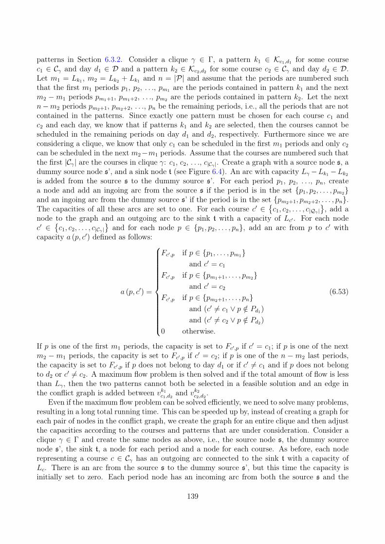
patterns in Section 6.3.2. Consider a clique γ ∈ Γ, a pattern k1 ∈ Kc1,d1 for some coursec1 ∈ Cγ and day d1 ∈ D and a pattern k2 ∈ Kc2,d2 for some course c2 ∈ Cγ and day d2 ∈ D.Let m1 = Lk1 , m2 = Lk2 + Lk1 and n = |P| and assume that the periods are numbered suchthat the first m1 periods p1, p2, . . ., pm1 are the periods contained in pattern k1 and the nextm2 −m1 periods pm1+1, pm1+2, . . ., pm2 are the periods contained in pattern k2. Let the nextn−m2 periods pm2+1, pm2+2, . . ., pn be the remaining periods, i.e., all the periods that are notcontained in the patterns. Since exactly one pattern must be chosen for each course c1 andc2 and each day, we know that if patterns k1 and k2 are selected, then the courses cannot bescheduled in the remaining periods on day d1 and d2, respectively. Furthermore since we areconsidering a clique, we know that only c1 can be scheduled in the first m1 periods and only c2

can be scheduled in the next m2−m1 periods. Assume that the courses are numbered such thatthe first |Cγ| are the courses in clique γ: c1, c2, . . ., c|Cγ |. Create a graph with a source node s, adummy source node s’, and a sink node t (see Figure 6.4). An arc with capacity Lγ−Lk1 −Lk2is added from the source s to the dummy source s’. For each period p1, p2, . . ., pn, createa node and add an ingoing arc from the source s if the period is in the set {p1, p2, . . . , pm2}and an ingoing arc from the dummy source s’ if the period is in the set {pm2+1, pm2+2, . . . , pn}.The capacities of all these arcs are set to one. For each course c′ ∈

{c1, c2, . . . , c|Qγ |

}, add a

node to the graph and an outgoing arc to the sink t with a capacity of Lc′ . For each nodec′ ∈

{c1, c2, . . . , c|Cγ |

}and for each node p ∈ {p1, p2, . . . , pn}, add an arc from p to c′ with

capacity a (p, c′) defined as follows:

a (p, c′) =

Fc′,p if p ∈ {p1, . . . , pm1}and c′ = c1

Fc′,p if p ∈ {pm1+1, . . . , pm2}and c′ = c2

Fc′,p if p ∈ {pm2+1, . . . , pn}and (c′ 6= c1 ∨ p /∈ Pd1)and (c′ 6= c2 ∨ p /∈ Pd2)

0 otherwise.

(6.53)

If p is one of the first m1 periods, the capacity is set to Fc′,p if c′ = c1; if p is one of the nextm2 −m1 periods, the capacity is set to Fc′,p if c′ = c2; if p is one of the n −m2 last periods,the capacity is set to Fc′,p if p does not belong to day d1 or if c′ 6= c1 and if p does not belongto d2 or c′ 6= c2. A maximum flow problem is then solved and if the total amount of flow is lessthan Lγ, then the two patterns cannot both be selected in a feasible solution and an edge inthe conflict graph is added between vk1c1,d2 and vk2c2,d2 .

Even if the maximum flow problem can be solved efficiently, we need to solve many problems,resulting in a long total running time. This can be speeded up by, instead of creating a graph foreach pair of nodes in the conflict graph, we create the graph for an entire clique and then adjustthe capacities according to the courses and patterns that are under consideration. Consider aclique γ ∈ Γ and create the same nodes as above, i.e., the source node s, the dummy sourcenode s’, the sink t, a node for each period and a node for each course. As before, each noderepresenting a course c ∈ Cγ has an outgoing arc connected to the sink t with a capacity ofLc. There is an arc from the source s to the dummy source s’, but this time the capacity isinitially set to zero. Each period node has an incoming arc from both the source s and the

139

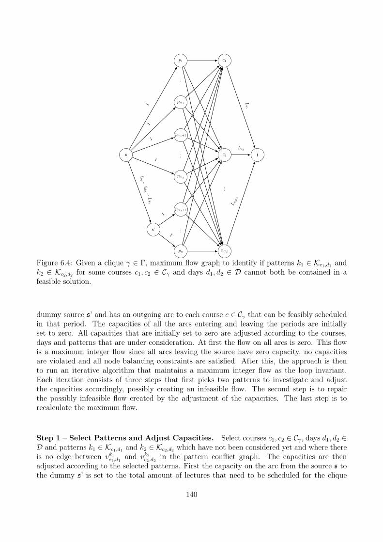
s ...

pm2

pm1+1

pm1

...

p1

pm2+1

...

pn

s’

c2

c1

...

c|Cγ |

t

Lγ −

Lk1 −

Lk2

1

1

1

1

1

1

Lc1

Lc2

Lc |C γ|

Figure 6.4: Given a clique γ ∈ Γ, maximum flow graph to identify if patterns k1 ∈ Kc1,d1 andk2 ∈ Kc2,d2 for some courses c1, c2 ∈ Cγ and days d1, d2 ∈ D cannot both be contained in afeasible solution.

dummy source s’ and has an outgoing arc to each course c ∈ Cγ that can be feasibly scheduledin that period. The capacities of all the arcs entering and leaving the periods are initiallyset to zero. All capacities that are initially set to zero are adjusted according to the courses,days and patterns that are under consideration. At first the flow on all arcs is zero. This flowis a maximum integer flow since all arcs leaving the source have zero capacity, no capacitiesare violated and all node balancing constraints are satisfied. After this, the approach is thento run an iterative algorithm that maintains a maximum integer flow as the loop invariant.Each iteration consists of three steps that first picks two patterns to investigate and adjustthe capacities accordingly, possibly creating an infeasible flow. The second step is to repairthe possibly infeasible flow created by the adjustment of the capacities. The last step is torecalculate the maximum flow.

Step 1 – Select Patterns and Adjust Capacities. Select courses c1, c2 ∈ Cγ, days d1, d2 ∈D and patterns k1 ∈ Kc1,d1 and k2 ∈ Kc2,d2 which have not been considered yet and where thereis no edge between vk1c1,d1 and vk2c2,d2 in the pattern conflict graph. The capacities are thenadjusted according to the selected patterns. First the capacity on the arc from the source s tothe dummy s’ is set to the total amount of lectures that need to be scheduled for the clique

140

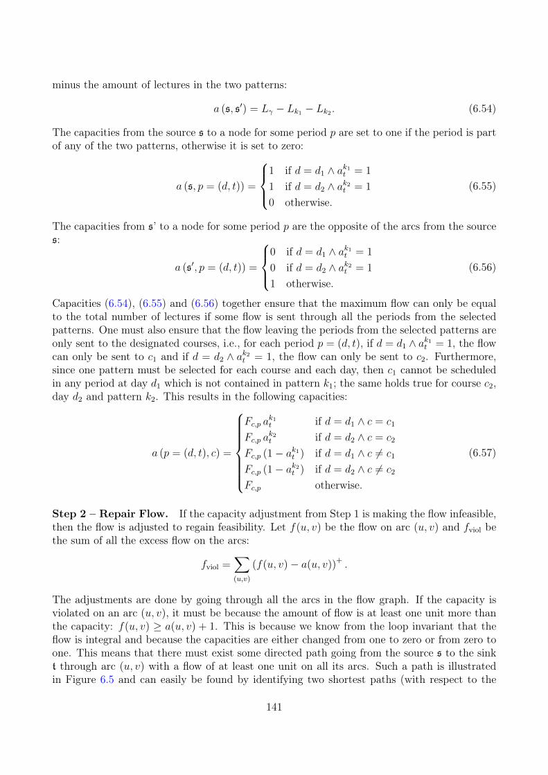
minus the amount of lectures in the two patterns:

a (s, s′) = Lγ − Lk1 − Lk2 . (6.54)

The capacities from the source s to a node for some period p are set to one if the period is partof any of the two patterns, otherwise it is set to zero:

a (s, p = (d, t)) =

1 if d = d1 ∧ ak1t = 1

1 if d = d2 ∧ ak2t = 1

0 otherwise.(6.55)

The capacities from s’ to a node for some period p are the opposite of the arcs from the sources:

a (s′, p = (d, t)) =

0 if d = d1 ∧ ak1t = 1

0 if d = d2 ∧ ak2t = 1

1 otherwise.(6.56)

Capacities (6.54), (6.55) and (6.56) together ensure that the maximum flow can only be equalto the total number of lectures if some flow is sent through all the periods from the selectedpatterns. One must also ensure that the flow leaving the periods from the selected patterns areonly sent to the designated courses, i.e., for each period p = (d, t), if d = d1 ∧ ak1t = 1, the flowcan only be sent to c1 and if d = d2 ∧ ak2t = 1, the flow can only be sent to c2. Furthermore,since one pattern must be selected for each course and each day, then c1 cannot be scheduledin any period at day d1 which is not contained in pattern k1; the same holds true for course c2,day d2 and pattern k2. This results in the following capacities:

a (p = (d, t), c) =

Fc,p ak1t if d = d1 ∧ c = c1

Fc,p ak2t if d = d2 ∧ c = c2

Fc,p (1− ak1t ) if d = d1 ∧ c 6= c1

Fc,p (1− ak2t ) if d = d2 ∧ c 6= c2

Fc,p otherwise.

(6.57)

Step 2 – Repair Flow. If the capacity adjustment from Step 1 is making the flow infeasible,then the flow is adjusted to regain feasibility. Let f(u, v) be the flow on arc (u, v) and fviol bethe sum of all the excess flow on the arcs:

fviol =∑(u,v)

(f(u, v)− a(u, v))+ .

The adjustments are done by going through all the arcs in the flow graph. If the capacity isviolated on an arc (u, v), it must be because the amount of flow is at least one unit more thanthe capacity: f(u, v) ≥ a(u, v) + 1. This is because we know from the loop invariant that theflow is integral and because the capacities are either changed from one to zero or from zero toone. This means that there must exist some directed path going from the source s to the sinkt through arc (u, v) with a flow of at least one unit on all its arcs. Such a path is illustratedin Figure 6.5 and can easily be found by identifying two shortest paths (with respect to the

141

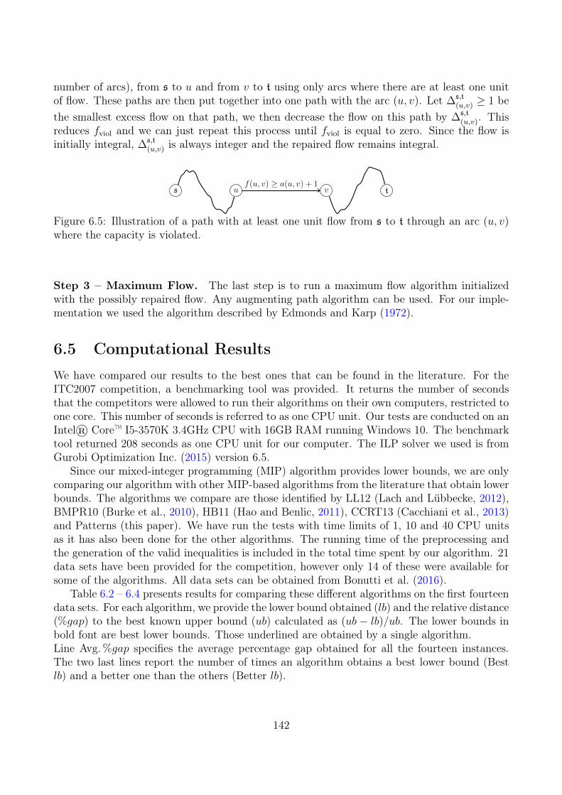
number of arcs), from s to u and from v to t using only arcs where there are at least one unitof flow. These paths are then put together into one path with the arc (u, v). Let ∆s,t

(u,v) ≥ 1 bethe smallest excess flow on that path, we then decrease the flow on this path by ∆s,t

(u,v). Thisreduces fviol and we can just repeat this process until fviol is equal to zero. Since the flow isinitially integral, ∆s,t

(u,v) is always integer and the repaired flow remains integral.

s u v tf(u, v) ≥ a(u, v) + 1

Figure 6.5: Illustration of a path with at least one unit flow from s to t through an arc (u, v)where the capacity is violated.

Step 3 – Maximum Flow. The last step is to run a maximum flow algorithm initializedwith the possibly repaired flow. Any augmenting path algorithm can be used. For our imple-mentation we used the algorithm described by Edmonds and Karp (1972).

6.5 Computational ResultsWe have compared our results to the best ones that can be found in the literature. For theITC2007 competition, a benchmarking tool was provided. It returns the number of secondsthat the competitors were allowed to run their algorithms on their own computers, restricted toone core. This number of seconds is referred to as one CPU unit. Our tests are conducted on anIntel® Core™ I5-3570K 3.4GHz CPU with 16GB RAM running Windows 10. The benchmarktool returned 208 seconds as one CPU unit for our computer. The ILP solver we used is fromGurobi Optimization Inc. (2015) version 6.5.

Since our mixed-integer programming (MIP) algorithm provides lower bounds, we are onlycomparing our algorithm with other MIP-based algorithms from the literature that obtain lowerbounds. The algorithms we compare are those identified by LL12 (Lach and Lübbecke, 2012),BMPR10 (Burke et al., 2010), HB11 (Hao and Benlic, 2011), CCRT13 (Cacchiani et al., 2013)and Patterns (this paper). We have run the tests with time limits of 1, 10 and 40 CPU unitsas it has also been done for the other algorithms. The running time of the preprocessing andthe generation of the valid inequalities is included in the total time spent by our algorithm. 21data sets have been provided for the competition, however only 14 of these were available forsome of the algorithms. All data sets can be obtained from Bonutti et al. (2016).

Table 6.2 – 6.4 presents results for comparing these different algorithms on the first fourteendata sets. For each algorithm, we provide the lower bound obtained (lb) and the relative distance(%gap) to the best known upper bound (ub) calculated as (ub − lb)/ub. The lower bounds inbold font are best lower bounds. Those underlined are obtained by a single algorithm.Line Avg.%gap specifies the average percentage gap obtained for all the fourteen instances.The two last lines report the number of times an algorithm obtains a best lower bound (Bestlb) and a better one than the others (Better lb).

142

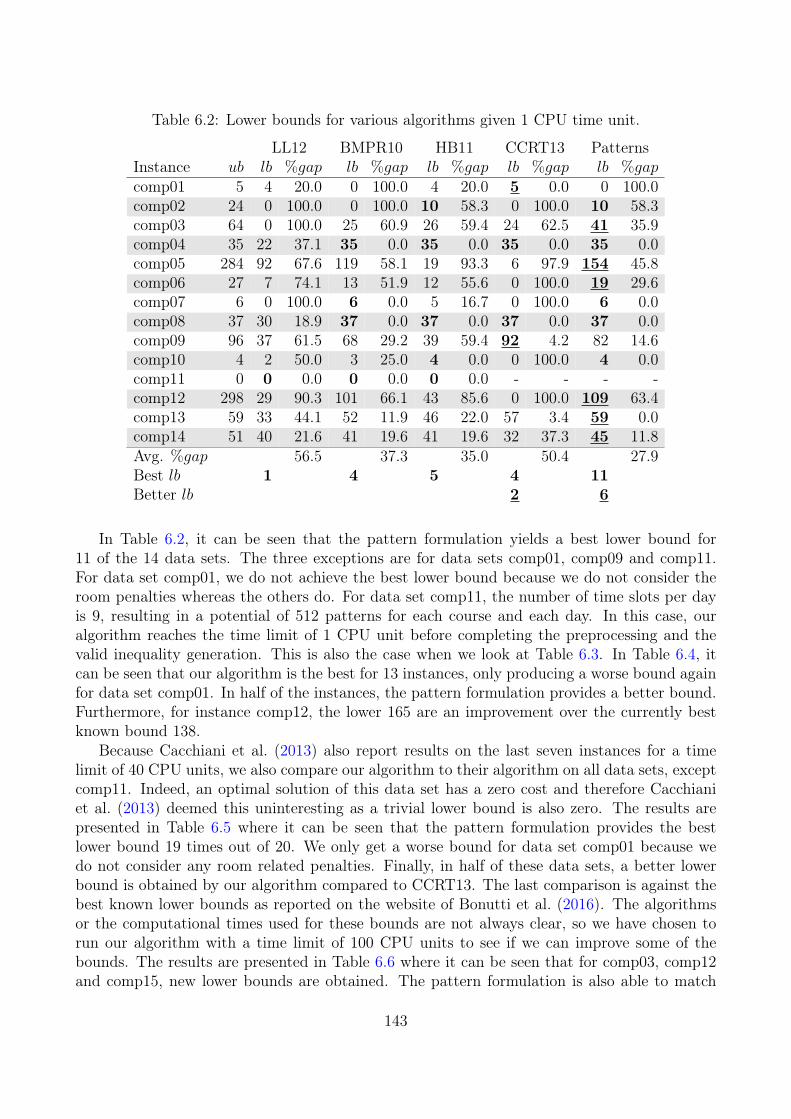
Table 6.2: Lower bounds for various algorithms given 1 CPU time unit.

LL12 BMPR10 HB11 CCRT13 PatternsInstance ub lb %gap lb %gap lb %gap lb %gap lb %gapcomp01 5 4 20.0 0 100.0 4 20.0 5 0.0 0 100.0comp02 24 0 100.0 0 100.0 10 58.3 0 100.0 10 58.3comp03 64 0 100.0 25 60.9 26 59.4 24 62.5 41 35.9comp04 35 22 37.1 35 0.0 35 0.0 35 0.0 35 0.0comp05 284 92 67.6 119 58.1 19 93.3 6 97.9 154 45.8comp06 27 7 74.1 13 51.9 12 55.6 0 100.0 19 29.6comp07 6 0 100.0 6 0.0 5 16.7 0 100.0 6 0.0comp08 37 30 18.9 37 0.0 37 0.0 37 0.0 37 0.0comp09 96 37 61.5 68 29.2 39 59.4 92 4.2 82 14.6comp10 4 2 50.0 3 25.0 4 0.0 0 100.0 4 0.0comp11 0 0 0.0 0 0.0 0 0.0 - - - -comp12 298 29 90.3 101 66.1 43 85.6 0 100.0 109 63.4comp13 59 33 44.1 52 11.9 46 22.0 57 3.4 59 0.0comp14 51 40 21.6 41 19.6 41 19.6 32 37.3 45 11.8Avg. %gap 56.5 37.3 35.0 50.4 27.9Best lb 1 4 5 4 11Better lb 2 6

In Table 6.2, it can be seen that the pattern formulation yields a best lower bound for11 of the 14 data sets. The three exceptions are for data sets comp01, comp09 and comp11.For data set comp01, we do not achieve the best lower bound because we do not consider theroom penalties whereas the others do. For data set comp11, the number of time slots per dayis 9, resulting in a potential of 512 patterns for each course and each day. In this case, ouralgorithm reaches the time limit of 1 CPU unit before completing the preprocessing and thevalid inequality generation. This is also the case when we look at Table 6.3. In Table 6.4, itcan be seen that our algorithm is the best for 13 instances, only producing a worse bound againfor data set comp01. In half of the instances, the pattern formulation provides a better bound.Furthermore, for instance comp12, the lower 165 are an improvement over the currently bestknown bound 138.

Because Cacchiani et al. (2013) also report results on the last seven instances for a timelimit of 40 CPU units, we also compare our algorithm to their algorithm on all data sets, exceptcomp11. Indeed, an optimal solution of this data set has a zero cost and therefore Cacchianiet al. (2013) deemed this uninteresting as a trivial lower bound is also zero. The results arepresented in Table 6.5 where it can be seen that the pattern formulation provides the bestlower bound 19 times out of 20. We only get a worse bound for data set comp01 because wedo not consider any room related penalties. Finally, in half of these data sets, a better lowerbound is obtained by our algorithm compared to CCRT13. The last comparison is against thebest known lower bounds as reported on the website of Bonutti et al. (2016). The algorithmsor the computational times used for these bounds are not always clear, so we have chosen torun our algorithm with a time limit of 100 CPU units to see if we can improve some of thebounds. The results are presented in Table 6.6 where it can be seen that for comp03, comp12and comp15, new lower bounds are obtained. The pattern formulation is also able to match

143

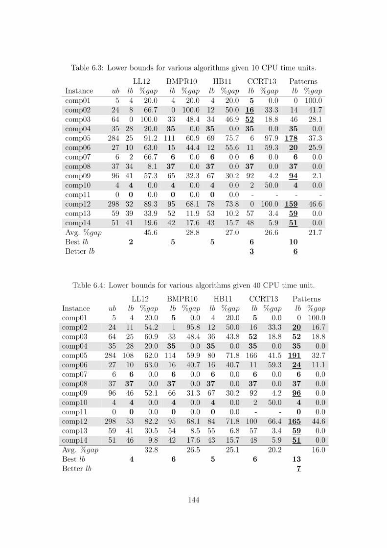
Table 6.3: Lower bounds for various algorithms given 10 CPU time units.

LL12 BMPR10 HB11 CCRT13 PatternsInstance ub lb %gap lb %gap lb %gap lb %gap lb %gapcomp01 5 4 20.0 4 20.0 4 20.0 5 0.0 0 100.0comp02 24 8 66.7 0 100.0 12 50.0 16 33.3 14 41.7comp03 64 0 100.0 33 48.4 34 46.9 52 18.8 46 28.1comp04 35 28 20.0 35 0.0 35 0.0 35 0.0 35 0.0comp05 284 25 91.2 111 60.9 69 75.7 6 97.9 178 37.3comp06 27 10 63.0 15 44.4 12 55.6 11 59.3 20 25.9comp07 6 2 66.7 6 0.0 6 0.0 6 0.0 6 0.0comp08 37 34 8.1 37 0.0 37 0.0 37 0.0 37 0.0comp09 96 41 57.3 65 32.3 67 30.2 92 4.2 94 2.1comp10 4 4 0.0 4 0.0 4 0.0 2 50.0 4 0.0comp11 0 0 0.0 0 0.0 0 0.0 - - - -comp12 298 32 89.3 95 68.1 78 73.8 0 100.0 159 46.6comp13 59 39 33.9 52 11.9 53 10.2 57 3.4 59 0.0comp14 51 41 19.6 42 17.6 43 15.7 48 5.9 51 0.0Avg. %gap 45.6 28.8 27.0 26.6 21.7Best lb 2 5 5 6 10Better lb 3 6

Table 6.4: Lower bounds for various algorithms given 40 CPU time unit.

LL12 BMPR10 HB11 CCRT13 PatternsInstance ub lb %gap lb %gap lb %gap lb %gap lb %gapcomp01 5 4 20.0 5 0.0 4 20.0 5 0.0 0 100.0comp02 24 11 54.2 1 95.8 12 50.0 16 33.3 20 16.7comp03 64 25 60.9 33 48.4 36 43.8 52 18.8 52 18.8comp04 35 28 20.0 35 0.0 35 0.0 35 0.0 35 0.0comp05 284 108 62.0 114 59.9 80 71.8 166 41.5 191 32.7comp06 27 10 63.0 16 40.7 16 40.7 11 59.3 24 11.1comp07 6 6 0.0 6 0.0 6 0.0 6 0.0 6 0.0comp08 37 37 0.0 37 0.0 37 0.0 37 0.0 37 0.0comp09 96 46 52.1 66 31.3 67 30.2 92 4.2 96 0.0comp10 4 4 0.0 4 0.0 4 0.0 2 50.0 4 0.0comp11 0 0 0.0 0 0.0 0 0.0 - - 0 0.0comp12 298 53 82.2 95 68.1 84 71.8 100 66.4 165 44.6comp13 59 41 30.5 54 8.5 55 6.8 57 3.4 59 0.0comp14 51 46 9.8 42 17.6 43 15.7 48 5.9 51 0.0Avg. %gap 32.8 26.5 25.1 20.2 16.0Best lb 4 6 5 6 13Better lb 7

144

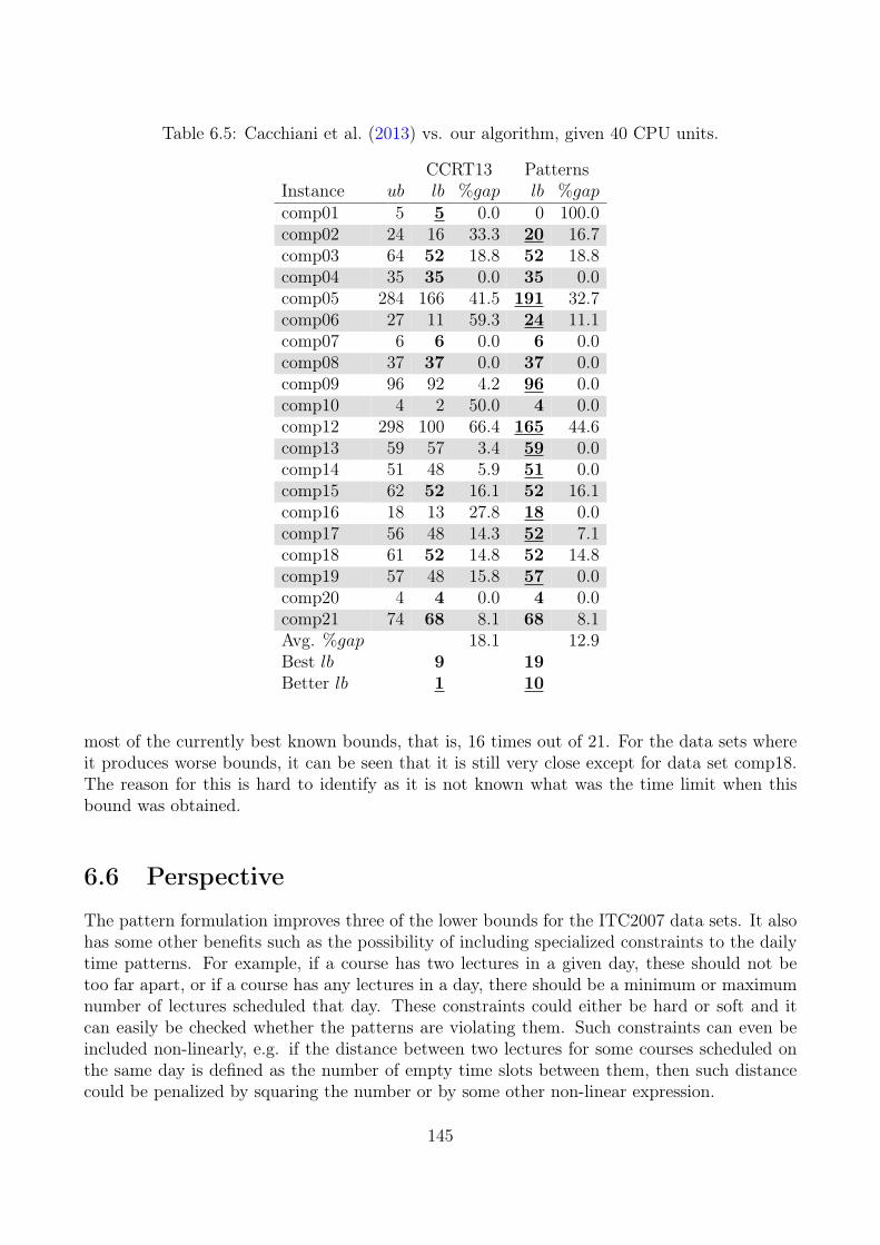
Table 6.5: Cacchiani et al. (2013) vs. our algorithm, given 40 CPU units.

CCRT13 PatternsInstance ub lb %gap lb %gapcomp01 5 5 0.0 0 100.0comp02 24 16 33.3 20 16.7comp03 64 52 18.8 52 18.8comp04 35 35 0.0 35 0.0comp05 284 166 41.5 191 32.7comp06 27 11 59.3 24 11.1comp07 6 6 0.0 6 0.0comp08 37 37 0.0 37 0.0comp09 96 92 4.2 96 0.0comp10 4 2 50.0 4 0.0comp12 298 100 66.4 165 44.6comp13 59 57 3.4 59 0.0comp14 51 48 5.9 51 0.0comp15 62 52 16.1 52 16.1comp16 18 13 27.8 18 0.0comp17 56 48 14.3 52 7.1comp18 61 52 14.8 52 14.8comp19 57 48 15.8 57 0.0comp20 4 4 0.0 4 0.0comp21 74 68 8.1 68 8.1Avg. %gap 18.1 12.9Best lb 9 19Better lb 1 10

most of the currently best known bounds, that is, 16 times out of 21. For the data sets whereit produces worse bounds, it can be seen that it is still very close except for data set comp18.The reason for this is hard to identify as it is not known what was the time limit when thisbound was obtained.

6.6 Perspective

The pattern formulation improves three of the lower bounds for the ITC2007 data sets. It alsohas some other benefits such as the possibility of including specialized constraints to the dailytime patterns. For example, if a course has two lectures in a given day, these should not betoo far apart, or if a course has any lectures in a day, there should be a minimum or maximumnumber of lectures scheduled that day. These constraints could either be hard or soft and itcan easily be checked whether the patterns are violating them. Such constraints can even beincluded non-linearly, e.g. if the distance between two lectures for some courses scheduled onthe same day is defined as the number of empty time slots between them, then such distancecould be penalized by squaring the number or by some other non-linear expression.

145

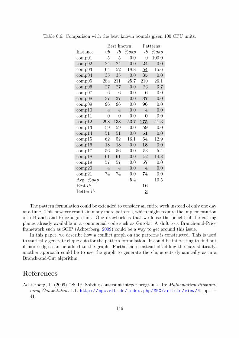
Table 6.6: Comparison with the best known bounds given 100 CPU units.

Best known PatternsInstance ub lb %gap lb %gapcomp01 5 5 0.0 0 100.0comp02 24 24 0.0 24 0.0comp03 64 52 18.8 54 15.6comp04 35 35 0.0 35 0.0comp05 284 211 25.7 210 26.1comp06 27 27 0.0 26 3.7comp07 6 6 0.0 6 0.0comp08 37 37 0.0 37 0.0comp09 96 96 0.0 96 0.0comp10 4 4 0.0 4 0.0comp11 0 0 0.0 0 0.0comp12 298 138 53.7 175 41.3comp13 59 59 0.0 59 0.0comp14 51 51 0.0 51 0.0comp15 62 52 16.1 54 12.9comp16 18 18 0.0 18 0.0comp17 56 56 0.0 53 5.4comp18 61 61 0.0 52 14.8comp19 57 57 0.0 57 0.0comp20 4 4 0.0 4 0.0comp21 74 74 0.0 74 0.0Avg. %gap 5.4 10.5Best lb 16Better lb 3

The pattern formulation could be extended to consider an entire week instead of only one dayat a time. This however results in many more patterns, which might require the implementationof a Branch-and-Price algorithm. One drawback is that we loose the benefit of the cuttingplanes already available in a commercial code such as Gurobi. A shift to a Branch-and-Priceframework such as SCIP (Achterberg, 2009) could be a way to get around this issue.

In this paper, we describe how a conflict graph on the patterns is constructed. This is usedto statically generate clique cuts for the pattern formulation. It could be interesting to find outif more edges can be added to the graph. Furthermore instead of adding the cuts statically,another approach could be to use the graph to generate the clique cuts dynamically as in aBranch-and-Cut algorithm.

ReferencesAchterberg, T. (2009). “SCIP: Solving constraint integer programs”. In: Mathematical Program-

ming Computation 1.1. http://mpc.zib.de/index.php/MPC/article/view/4, pp. 1–41.

146

Asín Achá, R. and Nieuwenhuis, R. (2012). “Curriculum-based course timetabling with SATand MaxSAT”. In: Annals of Operations Research, pp. 1–21.

Avella, P. and Vasil’ev, I. (2005). “A computational study of a cutting plane algorithm foruniversity course timetabling”. In: Journal of Scheduling. issn: 10946136. doi: 10.1007/s10951-005-4780-1.

Bettinelli, A., Cacchiani, V., Roberti, R., and Toth, P. (2015). “An overview of curriculum-basedcourse timetabling”. In: TOP, pp. 1–37.

Bonutti, A., De Cesco, F., Di Gaspero, L., and Schaerf, A. (2012). “Benchmarking curriculum-based course timetabling: Formulations, data formats, instances, validation, visualization,and results”. In: Annals of Operations Research 194.1, pp. 59–70.

Bonutti, A., Gaspero, L. D., and Schaerf, A. (2016). Curriculum-Based Course TimeTabling.http://tabu.diegm.uniud.it/ctt/index.php[Retrieved 30/12-2016].

Bron, C. and Kerbosch, J. (1973). “Algorithm 457: Finding All Cliques of an Undirected Graph”.In: Commun. ACM 16.9, pp. 575–577. issn: 0001-0782. doi: 10.1145/362342.362367. url:http://doi.acm.org/10.1145/362342.362367.

Burke, E. K., Mareček, J., Parkes, A. J., and Rudová, H. (2008). “Penalising Patterns in Timeta-bles: Novel Integer Programming Formulations”. In: Operations Research Proceedings 2007.Ed. by J. Kalcsics and S. Nickel. Vol. 2007. Operations Research Proceedings. 10.1007/978-3-540-77903-2_63. Springer Berlin Heidelberg, pp. 409–414. isbn: 978-3-540-77903-2.

Burke, E. K., Mareček, J., Parkes, A. J., and Rudová, H. (2010). “A supernodal formulation ofvertex colouring with applications in course timetabling”. In: Annals of Operations Research179.1, pp. 105–130.

Burke, E. K., Mareček, J., Parkes, A. J., and Rudová, H. (2012). “A branch-and-cut proce-dure for the Udine Course Timetabling problem”. In: Annals of Operations Research 194.1,pp. 71–87.

Cacchiani, V., Caprara, A., Roberti, R., and Toth, P. (2013). “A new lower bound for curriculum-based course timetabling”. In: Computers and Operation Research 40.10, pp. 2466–2477. doi:10.1016/j.cor.2013.02.010.

Di Gaspero, L., McCollum, B., and Schaerf, A. (2007). The Second International TimetablingCompetition (ITC-2007): Curriculum-based Course Timetabling (Track 3). Tech. rep. Schoolof Electronics, Electrical Engineering and Computer Science, Queenes University SARCBuilding, Belfast, United Kingdom.

Edmonds, J. and Karp, R. M. (1972). “Theoretical Improvements in Algorithmic Efficiency forNetwork Flow Problems”. In: J. ACM 19.2, pp. 248–264. issn: 0004-5411. doi: 10.1145/321694.321699. url: http://doi.acm.org.globalproxy.cvt.dk/10.1145/321694.321699.

Glover, F. and Laguna, M. (2013). “Handbook of Combinatorial Optimization”. In: ed. by M. P.Pardalos, D.-Z. Du, and L. R. Graham. New York, NY: Springer New York. Chap. TabuSearch, pp. 3261–3362. isbn: 978-1-4419-7997-1. doi: 10.1007/978-1-4419-7997-1\_17.url: http://dx.doi.org/10.1007/978-1-4419-7997-1%5C_17.

Gurobi Optimization Inc. (2015). Gurobi Optimizer Reference Manual. url: http://www.gurobi.com.

Hao, J. K. and Benlic, U. (2011). “Lower bounds for the ITC-2007 curriculum-based coursetimetabling problem”. In: European Journal of Operational Research 212.3, pp. 464–472.

147

Kou, L. T., Stockmeyer, L. J., andWong, C.-K. (1978). “Covering edges by cliques with regard tokeyword conflicts and intersection graphs”. In: Communications of the ACM 21.2, pp. 135–139.

Lach, G. and Lübbecke, M. (2012). “Curriculum based course timetabling: new solutions toUdine benchmark instances”. In: Annals of Operations Research 194, pp. 255–272. issn:0254-5330.

Lach, G. and Lübbecke, M. E. (2008). “Optimal University Course Timetables and the Par-tial Transversal Polytope”. In: International Workshop on Experimental and Efficient Algo-rithms. Springer, pp. 235–248.

McCollum, B., Schaerf, A., Paechter, B., McMullan, P., Lewis, R., Parkes, A. J., Gaspero, L. D.,Qu, R., and Burke, E. K. (2010). “Setting the Research Agenda in Automated Timetabling:The Second International Timetabling Competition”. In: INFORMS Journal on Computing22.1, pp. 120–130.

Van Roy, T. J. and Wolsey, L. A. (1987). “Solving mixed integer programming problems usingautomatic reformulation”. In: Operations Research 35.1, pp. 45–57.

148

7 Dantzig-Wolfe Decomposition of theDaily Course Pattern Formulation forCurriculum-based Course Timetabling

Niels-Christian F. Baggera,b · Matias Sørensena,b · Thomas R. Stidsena

amORetime research group, Management Science, Department of Management Engineering,Technical University of Denmark, Produktionstorvet, Building 426B, DK-2800 Kgs. Lyngby,Denmark, http://www.moretime.man.dtu.dk/

bMaCom A/S, Vesterbrogade 48, 1., DK-1620 København V, Denmark

Status: Submitted to European Journal of Operational Research

Abstract: In this paper, we consider the Curriculum-based Course Timetablingproblem, which consists of assigning weekly lectures to a time schedule and assignthem to rooms. We develop a Column Generation algorithm based on a patternformulation of the time scheduling part of the problem. The pattern formulation isan enumeration of all schedules to which each course can be assigned on each day,and it is a lower bounding model. We apply a Dantzig-Wolfe Decomposition thatexploits the block diagonal structure of the pattern formulation such that we havea pricing problem for each day.

We provide a preprocessing technique that on average removes more than 40%of the pattern variables of the pricing problems. We then extend the preprocessingtechnique into inequalities that we add to the model. Lastly, we describe howwe apply Local Branching to the pricing problem by using columns generated inprevious iterations.

We compare the lower bounds we obtain with other methods from literature on20 data instances originating from real-world applications. For 16 of the instancesthe optimal solutions are known, but the remaining four are still open. The averagegap between the lower bounds obtained and the best-known solutions is lower thanthe other approaches from the literature, except the pattern formulation from whichthe decomposition originates from. However, our approach is able to improve thebest-known lower bound for all four open instances, which decreases the averagegap from 24% to 11%.

149

Keywords: Timetabling · Integer Programming · Education · Column Genera-tion · Local Branching

7.1 IntroductionIn this article we focus on the Curriculum-based Course Timetabling problem (CTT) as de-scribed by Di Gaspero et al. (2007). The problem has received much attention as it was used forthe second International Timetabling Competition in 2007 (ITC2007) (Di Gaspero et al., 2007;McCollum et al., 2010). Following the competition, a website (The Scheduling and TimetablingResearch Group at the University of Udine, Italy, 2015) has been created where researchers canupload data instances, solutions and bounds. Most of the work conducted on CTT is dominatedby heuristic approaches (Asín Aschá and Nieuwenhuis, 2014; Lübbecke, 2015). These heuristicmethods have provided most of the best-known solutions according to the website The Schedul-ing and Timetabling Research Group at the University of Udine, Italy (2015). For ITC200721 data instances were provided arising from real-world applications. Four of these instancesare still open, meaning that the best-known upper bound does not equal the best-known lowerbound. The lower bounds are necessary as the heuristics themselves do not provide a qualitymeasurement. Our goal of this work is to strengthen the best-known lower bounds. We dothis by applying a Dantzig-Wolfe decomposition of a previous formulation which is solved bycolumn generation. Column generation approaches have been considered before by Cacchianiet al. (2013), but it is still worthwhile to investigate such methods further (Lübbecke, 2015).

In section 7.1.1 we describe the problem in details, and in section 7.1.2 we provide anoverview of other methods in literature that have considered CTT. In section 7.2 we describethe pattern formulation suggested by Bagger et al. (2016) as this model is the basis of ourwork in this article. We assume that the reader is familiar with Dantzig-Wolfe Decompositionand Column Generation. However, in section 7.3 we provide a brief overview of the techniquesfollowed by our application of the decomposition of the pattern formulation. In section 7.4 wedescribe the preprocessing techniques we apply, as well as some inequalities we derive followedby the framework we use in the solution process; Local Branching (Fischetti and Lodi, 2003).We report the results of our computational experiments in section 7.5, and lastly, we provideour conclusion in section 7.6.

7.1.1 Curriculum-based Course Timetabling

The CTT problem consists of the following entities; courses, days, time slots, lecturers, roomsand curricula. Each course is taught by exactly one lecturer and contains lectures that mustall be scheduled in a weekly timetable and assigned to rooms. The week is divided into days,and each day is divided into time slots which are all equal in size. A day and time slot pair isreferred to as a period, so the total number of periods is the number of days multiplied by thenumber of time slots. The length of one lecture corresponds to one period. A curriculum is aset of courses where for every pair there is a set of students attending both courses.

The hard constraints are as follows: All lectures of a course must be scheduled, and theymust be scheduled in different periods. If a lecture is not scheduled, then it is counted as oneviolation of the Lectures (L) constraint, and if two lectures of the same course are scheduled inthe same period, then this is also counted as one violation. A course can have specific periods

150

defined as unavailable periods. Every lecture scheduled in such a period is considered as oneviolation of the Availability (A) constraint. The constraint Conflicts (C) is violated by oneif two courses that are taught by the same lecturer or belonging to the same curriculum havelectures scheduled in the same periods. Every room cannot accommodate more than one lecturein any given period. If more than one lecture is scheduled in the same room and same period,then the constraint Room Occupancy (RO) is violated by one for every lecture minus one.

Besides the hard constraints, the problem also contains four soft constraints. We are allowedto schedule any course into any room. However, it is desired to be able to accommodate asmany students as possible when scheduling the courses into rooms. Every room has a capacity,and if the number of students attending a lecture is larger than the capacity of the room thatthe lecture is assigned, the constraint Room Capacity (RC) is violated by one for each studentmore than the capacity. Furthermore, as the courses contain multiple lectures, it can also bean advantage that the lectures are all scheduled in the same room during the week. For everycourse the constraint Room Stability (RStab) is violated by one for every distinct room towhich the course is assigned minus one. For every course it is preferred to spread the lecturesacross a predetermined number of days. This number is called minimum working days. Ifthe lectures are scheduled in fewer days than the minimum working days, then the constraintMinimum Working Days (MWD) is violated by one for each day below the minimum workingdays on which the lectures are scheduled. The last soft constraint is the Isolated Lectures (IL)constraint. If two periods belong to the same day and are in consecutive time slots, then we saythat the periods are adjacent. Consider a curriculum and a course belonging to the curriculum.If the course has a lecture scheduled in a period and no lecture from any of the courses belongingto the curriculum has a lecture scheduled in an adjacent period, then we say that the lectureis isolated. For every curriculum, the constraint Isolated Lectures (IL) is violated by one forevery isolated lecture.

Note that the IL constraint is usually referred to as the curriculum compactness constraintin literature. We use the name isolated lectures as Bonutti et al. (2012) mentions different waysof defining curriculum compactness, and they use the name isolated lectures for the formulationused here and in ITC2007.

Any feasible timetable must fulfil all the hard constraints, i.e., a timetable is consideredfeasible if, and only if, all the hard constraints have no violations. The objective is then to finda feasible timetable while minimising the soft constraints. Each soft constraint has a weightassociated such that a single objective is defined by a weighted sum of all the soft constraints.

7.1.2 Related Work

In this section, we describe approaches from literature that have considered CTT. As ourmethod is a lower bounding method, we focus on other lower bounding methods for CTT inliterature. For a comprehensive overview of the literature regarding CTT, we refer to Bettinelliet al. (2015).

Burke et al. (2010a) introduce an exact mixed integer programming (MIP) model of CTT.They formulate the IL by using a variable for each curriculum and each period. Burke et al.(2008) remove those variables and instead they have just one variable for each curriculum andeach day. The value of this variable is then calculated by adding exponentially many constraints.In Burke et al. (2012) they keep a subset of the beforementioned constraints and then add the

151

remaining dynamically whenever they are violated. Burke et al. (2010b) take the model fromBurke et al. (2010a) and split it into two stages; first the courses are scheduled into periodsand then they are assigned to rooms. This approach is executed iteratively.

Splitting the problem into two stages is also considered by Lach and Lübbecke (2008) andLach and Lübbecke (2012), where the problem is also split into two stages; the first stageschedules the courses to periods and assign them to capacities, and the second stage thenassigns the rooms with respect to the assigned capacities.

Hao and Benlic (2011) consider the first stage problem of Lach and Lübbecke (2012). Theymake a decomposition by relaxing some of the constraints such that the problem can be dividedinto subproblems. They then compute a lower bound for each subproblem and sum them upto get a lower bound for the overall problem.

Cacchiani et al. (2013) also compute lower bounds. They do this by splitting the probleminto two parts, where one part considers the time related constraints and the other part considersthe room related constraints. A lower bound is then calculated by summing up lower boundsfor both parts. They, therefore, apply a Dantzig-Wolfe decomposition of the part with the timerelated constraints such that the pricing problem is decomposable by days and the model issolved by column generation.

Asín Aschá and Nieuwenhuis (2014) propose multiple satisfiability encodings. They start bytreating the soft constraints as hard constraints and solve the problem as a pure satisfiabilityproblem. Then they relax the constraints one by one, to move towards a weighted partialmaximum satisfiability encoding.

In Bagger et al. (2017) a decomposition of the problem is considered similar to Lach andLübbecke (2012) and Burke et al. (2010b) where the problem is split into a time schedulingmodel and a room allocation model. The two models are then reconnected by an underlyingflow problem to get an exact formulation.

In Bagger et al. (2016) the time scheduling part of the problem is considered. Here a patternformulation is suggested where each variable corresponds to a time schedule for one course onone day.

In this article we apply Dantzig-Wolfe decomposition to the pattern formulation in Baggeret al. (2016). The decomposition makes the pricing problem decomposable by days, and wesolve the problem by a column generation algorithm. Note that this is similar to the workby Cacchiani et al. (2013). Cacchiani et al. (2013) apply the decomposition on the basis ofa formulation where the main decision variables each represent one course and one period.Furthermore, the formulation does not guarantee a feasible schedule, i.e., some of the hardconstraints can be violated. We apply the decomposition on the pattern formulation describedin Bagger et al. (2016) which is an extensive model where each variable represents an entireschedule for one course on one day. Furthermore, the formulation ensures that none of the hardconstraints is violated.

7.2 Pattern FormulationIn this section we provide an overview of the pattern formulation provided by Bagger et al.(2016), which we refer to for details. The idea of the pattern formulation is to have a binaryvariable represent an entire schedule for a course on one day. This formulation contains anexponential number of variables. However, as most of the data instances used in literature have

152

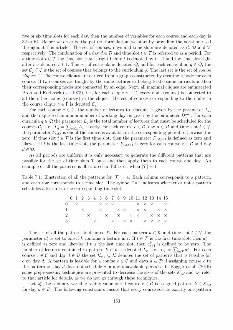
five or six time slots for each day, then the number of variables for each course and each day is32 or 64. Before we describe the pattern formulation, we start by providing the notation usedthroughout this article. The set of courses, days and time slots are denoted as C, D and Trespectively. The combination of a day d ∈ D and time slot t ∈ T is referred to as a period. Fora time slot t ∈ T the time slot that is right before t is denoted by t− 1 and the time slot rightafter t is denoted t+ 1. The set of curricula is denoted Q, and for each curriculum q ∈ Q, theset Cq ⊆ C is the set of courses that belongs to the curriculum q. The last set is the set of coursecliques Γ. The course cliques are derived from a graph constructed by creating a node for eachcourse. If two courses are taught by the same lecturer or belong to the same curriculum, thentheir corresponding nodes are connected by an edge. Next, all maximal cliques are enumeratedBron and Kerbosch (see 1973), i.e., for each clique γ ∈ Γ, every node (course) is connected toall the other nodes (courses) in the clique. The set of courses corresponding to the nodes inthe course clique γ ∈ Γ is denoted Cγ.

For each course c ∈ C, the number of lectures to schedule is given by the parameter Lc,and the requested minimum number of working days is given by the parameter Dmin

c . For eachcurricula q ∈ Q the parameter Lq is the total number of lectures that must be scheduled for thecourses Cq, i.e., Lq =

∑c∈Cq Lc. Lastly, for each course c ∈ C, day d ∈ D and time slot t ∈ T

the parameter Fc,d,t is one if the course is available in the corresponding period, otherwise it iszero. If time slot t ∈ T is the first time slot, then the parameter Fc,d,t−1 is defined as zero andlikewise if t is the last time slot, the parameter Fc,d,t+1 is zero for each course c ∈ C and dayd ∈ D.

As all periods are uniform it is only necessary to generate the different patterns that arepossible for the set of time slots T once and then apply them to each course and day. Anexample of all the patterns is illustrated in Table 7.1 when |T | = 4.

Table 7.1: Illustration of all the patterns for |T | = 4. Each column corresponds to a pattern,and each row corresponds to a time slot. The symbol ”×” indicates whether or not a patternschedules a lecture in the corresponding time slot.

0 1 2 3 4 5 6 7 8 9 10 11 12 13 14 150 × × × × × × × ×1 × × × × × × × ×2 × × × × × × × ×3 × × × × × × × ×

The set of all the patterns is denoted K. For each pattern k ∈ K and time slot t ∈ T theparameter akt is set to one if k contains a lecture in t. If t ∈ T is the first time slot, then akt−1

is defined as zero and likewise if t is the last time slot, then akt+1 is defined to be zero. Thenumber of lectures contained in pattern k ∈ K is denoted Lk, i.e., Lk =

∑t∈T a

kt . For each

course c ∈ C and day d ∈ D the set Kc,d ⊆ K denotes the set of patterns that is feasible forc on day d. A pattern is feasible for a course c ∈ C and days d ∈ D if assigning course c tothe pattern on day d does not schedule c in any unavailable periods. In Bagger et al. (2016)some preprocessing techniques are presented to decrease the sizes of the sets Kc,d and we referto that article for details, as we do not go through these techniques.

Let λkc,d be a binary variable taking value one if course c ∈ C is assigned pattern k ∈ Kc,dfor day d ∈ D. The following constraints ensure that every course selects exactly one pattern

153

for each day, that all lectures are scheduled, and that no more than one lecture is scheduled inany room in any period:

∑k∈Kc,d

λkc,d = 1, ∀c ∈ C, d ∈ D (7.1)

∑d∈D,k∈Kc,d

Lkλkc,d = Lc, ∀c ∈ C (7.2)

∑c∈C,k∈Kc,d

akt λkc,d ≤ R, ∀d ∈ D, t ∈ T (7.3)

The constraints (7.1) – (7.3) ensure that the constraints A, L and RO are not violated. Tomodel constraint C a pattern conflict graph G = (V , E) is constructed. For every course c ∈ C,day d ∈ D and pattern k ∈ Kc,d there is a node vkc,d ∈ V corresponding to the variable λkc,d. Ifcourse c1 ∈ C chooses pattern k1 ∈ Kc1,d1 for day d1 ∈ D and course c2 ∈ C chooses patternk2 ∈ Kc2,d2 for day d2 ∈ D and this results in a conflict, then there is an edge e ∈ E betweenthe two nodes vk1c1,d1 and vk2c2,d2 . These conflicts contain the C constraints, and in Bagger et al.(2016) more conflicts are identified to add more edges to the graph. A clique in the graph is asubgraph of the graph such that every node in this subgraph is connected by an edge to everyother node in the subgraph. Let Θ be a set of cliques such that for each edge (u, v) ∈ E boththe nodes u and v are contained in at least one clique. We refer to these cliques as patterncliques to be able to distinct them from the course cliques Γ. For each pattern clique θ ∈ Θ inthe graph let Vθ be the set of nodes in the clique. Adding the following constraints ensure thatthe C constraints are not violated: ∑

vkc,d∈Vθ

λkc,d ≤ 1, ∀θ ∈ Θ (7.4)

Let wc be an integer variable calculating how much the soft constraint MWD is violated.The value of these variables can be calculated by the following constraints:∑

d∈D,k∈Kc,d:Lc≥1

λkc,d + wc ≥ Dminc , ∀c ∈ C (7.5)

To calculate the violation of the soft constraint IL the parameter akt is defined for eachpattern k ∈ K and time slot t ∈ T :

akt := akt −max{akt−1, a

kt+1

}, k ∈ K, t ∈ T (7.6)

The variable sq,d,t is introduced for each curriculum q ∈ Q, day d ∈ D and time slot t ∈ T .The variable sq,d,t is a binary variable that takes value one if q has an isolated lecture in timeslot t for day d: ∑

c∈Cq ,k∈Kc,d

akt λkc,d ≤ sq,d,t, ∀q ∈ Q, d ∈ D, t ∈ T (7.7)

154

Let WMWD and W IL be the non-negative weights of the soft constraints MWD and ILrespectively. Then the objective function to minimize can be formulated as follows:∑

q∈Q,d∈D,t∈T

W ILsq,d,t +∑c∈C

WMWDwc (7.8)

It was shown by Bagger et al. (2016) that if Dminc = Lc or Dmin

c = 2, then the followingsubstitutions can be made:

wc =∑d∈D,

k∈Kc,d:Lk≥2

(Lk − 1)λkc,d, ∀c ∈ C : Dminc = Lc (7.9)

wc =∑d∈D,

k∈Kc,d:Lk=Lc

λkc,d, ∀c ∈ C : Dminc = 2 (7.10)

Consider a curriculum q ∈ Q, a day d ∈ D and time slot t ∈ T . Let the set of courses Cq,d,tbe defined as follows:

Cq,d,t :=

c ∈ Cq∣∣∣∣∣∣

∑t′∈{t−1,t,t+1}

Fc,d,t′ ≥ 1

(7.11)

It was shown by Bagger et al. (2016) that if the number of courses in Cq,d,t is one, thefollowing substitution can be made:

sq,d,t =∑

c∈Cq ,k∈Kc,d:

akt=1∧akt−1=akt+1=0

λkc,d,∀q ∈ Q, d ∈ D,∈ T : |Cq,d,t| = 1 (7.12)

Bagger et al. (2016) also describes valid inequalities that are added to the model. We do notgo through them here, but we refer to that article for details. In this article, we do one morepreprocessing that is not described in Bagger et al. (2016). We consider the model includingall the valid inequalities, but excluding the w and s variables and their associated constraints,i.e., we only consider the feasibility part of the model. We then iterate through each variableλkc,d and set the lower bound to one. Then we solve the LP relaxation, and if it is infeasible,we remove the variable from the model. Otherwise, we change the lower bound of λkc,d back tozero.

7.3 Dantzig-Wolfe Decomposition

In this section we provide a brief description of Dantzig-Wolfe decomposition followed by ourapplication. In section 7.3.1 an introduction to the Dantzig-Wolfe decomposition for MixedInteger Programs (MIP) is given, and in section 7.3.2 we describe how we apply it to thepattern formulation of CTT.

155

7.3.1 Brief Introduction to Dantzig-Wolfe Decomposition

Our introduction to the Dantzig-Wolfe Decomposition is specific for MIP models and we refer toMartin (1999, chapter 11) and Desrosiers and Lübbecke (2010) for thorough and more generaldescriptions. We consider an MIP of the form:

min c>x (7.13)s.t. Ax ≥ b (7.14)

Bx ≥ d (7.15)x ∈ Zn (7.16)

where c, x, b and d are vectors and A and B are matrices. To get a lower bound of the model(7.13) – (7.16) the linear programming (LP) relaxation is solved. In Figure 7.1 an example ofthe solution space is illustrated.

Ax ≥ b Bx ≥ d

LP solution spaceInteger solution

Figure 7.1: Illustration of the solution space.

The idea of the Dantzig-Wolfe decomposition for an MILP is to take the convex hull of{x ∈ X |Bx ≥ d}, and replace it by variables. For simplicity, we assume that the convex hullconv ({x ∈ X |Bx ≥ d}) is a polytope. Then any point x in this polytope can be written as aconvex combination of the extreme points, i.e., if

{xh}h∈H is the set of all the extreme points

of conv ({x ∈ R |Bx ≥ d}), then x can be written as follows:

156

∑h∈H

xhλh = x (7.17)∑h∈H

λh = 1 (7.18)

λh ≥ 0, ∀h ∈ H (7.19)

We can take this representation and insert it into the LP-relaxation of the model (7.13) –(7.16):

min∑h∈H

(c>xh

)λh (7.20)

s.t.∑h∈H

(Axh

)λh ≥ b (7.21)∑

h∈H

λh = 1 (7.22)

λh ≥ 0, ∀h ∈ H (7.23)

Model (7.20) – (7.23) is referred to as the LP relaxation of the Dantzig-Wolfemaster problem.Let z∗IP be the optimal objective value of the model (7.13) – (7.16), let z∗LP be the optimalobjective value of the LP relaxation of the same model and let z∗DW be the optimal objectivevalue of the model (7.20) – (7.23). Then the benefit of rewriting the model is that the LPrelaxation of the Dantzig-Wolfe master problem is a stronger relaxation in the sense that wehave the following relation:

z∗LP ≤ z∗DW ≤ z∗IP (7.24)

Figure 7.2 illustrates the impact on the solution space when Bx ≥ d from Figure 7.1 isreplaced by conv ({Bx ≥ d, x ∈ Zn}).

Explicitly describing model (7.20) – (7.23) can be difficult as the number of extreme pointsin conv ({x ∈ X |Bx ≥ d}) can be exponentially large. So a way to solve the model is to startwith a restricted set H′ ⊆ H and then solve the model (7.20) – (7.23) with this restricted set.The model with this restricted set is referred to as the restricted master problem (RMP). Letπ be the dual vector of the constraints (7.21) and π0 be the dual variable of constraint (7.22).For a dual solution (π, π0) the reduced cost of a column h ∈ H is ch = (c − A>π)>xh − π0. Ifthe dual solution is optimal then the RMP is optimal when ch ≥ 0 for every h ∈ H. We knowthat ch ≥ 0 for every h ∈ H′, but there may exist some column h ∈ H\H′ where ch < 0 so weneed to check if any such column exist. This can be done by solving the following problem,known as the pricing problem (PP):

min (c− A>π)>x− π0 (7.25)s.t. Bx ≥ d (7.26)

x ∈ Zn (7.27)

157

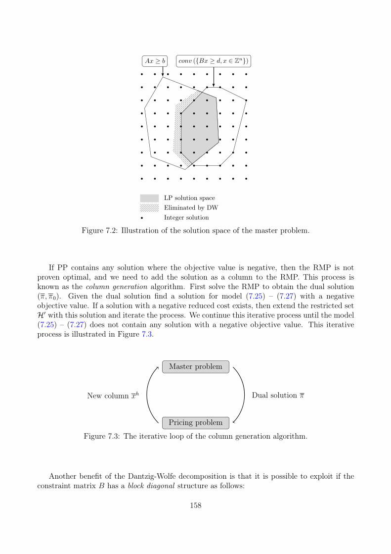
Ax ≥ b conv ({Bx ≥ d, x ∈ Zn})

LP solution spaceEliminated by DWInteger solution

Figure 7.2: Illustration of the solution space of the master problem.

If PP contains any solution where the objective value is negative, then the RMP is notproven optimal, and we need to add the solution as a column to the RMP. This process isknown as the column generation algorithm. First solve the RMP to obtain the dual solution(π, π0). Given the dual solution find a solution for model (7.25) – (7.27) with a negativeobjective value. If a solution with a negative reduced cost exists, then extend the restricted setH′ with this solution and iterate the process. We continue this iterative process until the model(7.25) – (7.27) does not contain any solution with a negative objective value. This iterativeprocess is illustrated in Figure 7.3.

Master problem

Pricing problem

Dual solution πNew column xh

Figure 7.3: The iterative loop of the column generation algorithm.

Another benefit of the Dantzig-Wolfe decomposition is that it is possible to exploit if theconstraint matrix B has a block diagonal structure as follows:

158

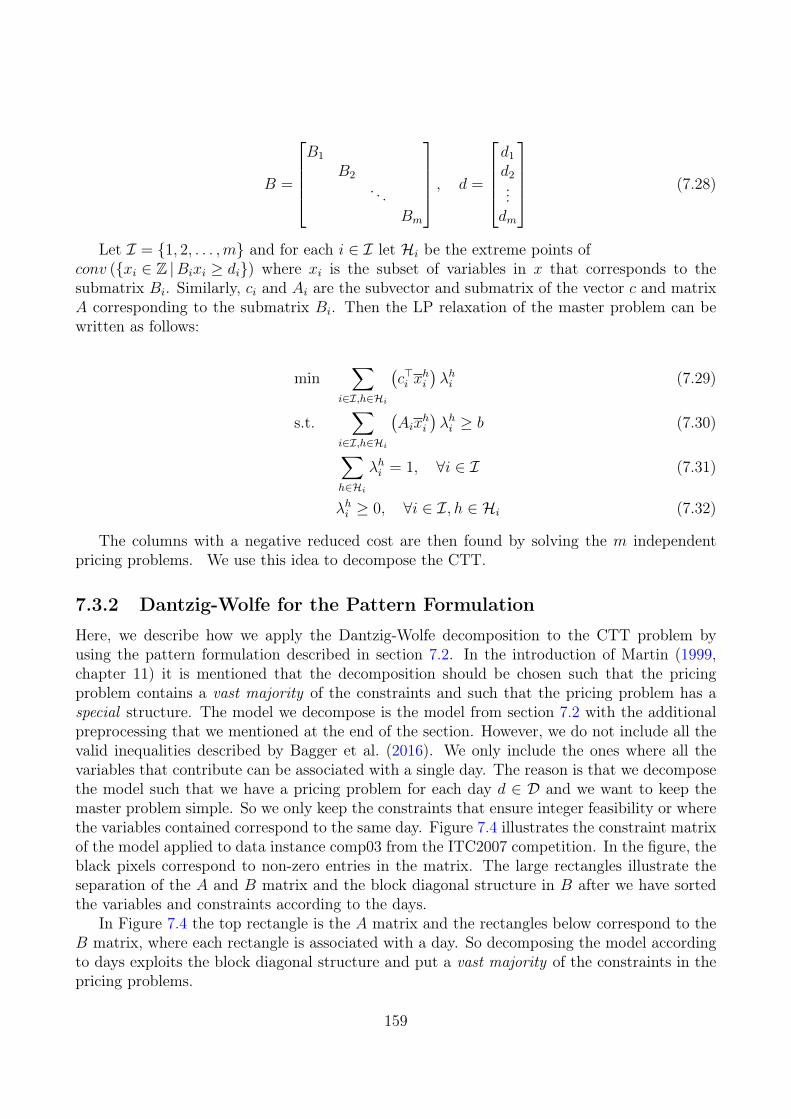
B =

B1

B2

. . .Bm

, d =

d1

d2...dm

(7.28)

Let I = {1, 2, . . . ,m} and for each i ∈ I let Hi be the extreme points ofconv ({xi ∈ Z |Bixi ≥ di}) where xi is the subset of variables in x that corresponds to thesubmatrix Bi. Similarly, ci and Ai are the subvector and submatrix of the vector c and matrixA corresponding to the submatrix Bi. Then the LP relaxation of the master problem can bewritten as follows:

min∑

i∈I,h∈Hi

(c>i x

hi

)λhi (7.29)

s.t.∑

i∈I,h∈Hi

(Aix

hi

)λhi ≥ b (7.30)∑

h∈Hi

λhi = 1, ∀i ∈ I (7.31)

λhi ≥ 0, ∀i ∈ I, h ∈ Hi (7.32)

The columns with a negative reduced cost are then found by solving the m independentpricing problems. We use this idea to decompose the CTT.

7.3.2 Dantzig-Wolfe for the Pattern Formulation

Here, we describe how we apply the Dantzig-Wolfe decomposition to the CTT problem byusing the pattern formulation described in section 7.2. In the introduction of Martin (1999,chapter 11) it is mentioned that the decomposition should be chosen such that the pricingproblem contains a vast majority of the constraints and such that the pricing problem has aspecial structure. The model we decompose is the model from section 7.2 with the additionalpreprocessing that we mentioned at the end of the section. However, we do not include all thevalid inequalities described by Bagger et al. (2016). We only include the ones where all thevariables that contribute can be associated with a single day. The reason is that we decomposethe model such that we have a pricing problem for each day d ∈ D and we want to keep themaster problem simple. So we only keep the constraints that ensure integer feasibility or wherethe variables contained correspond to the same day. Figure 7.4 illustrates the constraint matrixof the model applied to data instance comp03 from the ITC2007 competition. In the figure, theblack pixels correspond to non-zero entries in the matrix. The large rectangles illustrate theseparation of the A and B matrix and the block diagonal structure in B after we have sortedthe variables and constraints according to the days.

In Figure 7.4 the top rectangle is the A matrix and the rectangles below correspond to theB matrix, where each rectangle is associated with a day. So decomposing the model accordingto days exploits the block diagonal structure and put a vast majority of the constraints in thepricing problems.

159

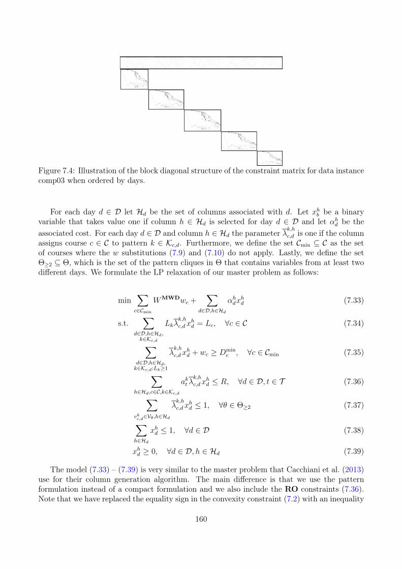
Figure 7.4: Illustration of the block diagonal structure of the constraint matrix for data instancecomp03 when ordered by days.

For each day d ∈ D let Hd be the set of columns associated with d. Let xhb be a binaryvariable that takes value one if column h ∈ Hd is selected for day d ∈ D and let αhd be theassociated cost. For each day d ∈ D and column h ∈ Hd the parameter λk,hc,d is one if the columnassigns course c ∈ C to pattern k ∈ Kc,d. Furthermore, we define the set Cmin ⊆ C as the setof courses where the w substitutions (7.9) and (7.10) do not apply. Lastly, we define the setΘ≥2 ⊆ Θ, which is the set of the pattern cliques in Θ that contains variables from at least twodifferent days. We formulate the LP relaxation of our master problem as follows:

min∑c∈Cmin

WMWDwc +∑

d∈D,h∈Hd

αhdxhd (7.33)

s.t.∑

d∈D,h∈Hd,k∈Kc,d

Lkλk,h

c,dxhd = Lc, ∀c ∈ C (7.34)

∑d∈D,h∈Hd,k∈Kc,d:Lk≥1

λk,h

c,dxhd + wc ≥ Dmin

c , ∀c ∈ Cmin (7.35)

∑h∈Hd,c∈C,k∈Kc,d

akt λk,h

c,dxhd ≤ R, ∀d ∈ D, t ∈ T (7.36)

∑vkc,d∈Vθ,h∈Hd

λk,h

c,dxhd ≤ 1, ∀θ ∈ Θ≥2 (7.37)

∑h∈Hd

xhd ≤ 1, ∀d ∈ D (7.38)

xhd ≥ 0, ∀d ∈ D, h ∈ Hd (7.39)

The model (7.33) – (7.39) is very similar to the master problem that Cacchiani et al. (2013)use for their column generation algorithm. The main difference is that we use the patternformulation instead of a compact formulation and we also include the RO constraints (7.36).Note that we have replaced the equality sign in the convexity constraint (7.2) with an inequality

160

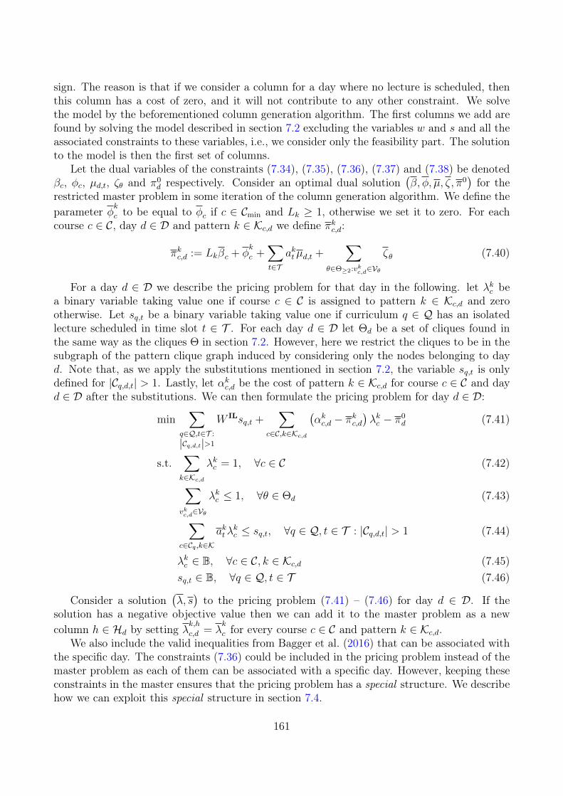
sign. The reason is that if we consider a column for a day where no lecture is scheduled, thenthis column has a cost of zero, and it will not contribute to any other constraint. We solvethe model by the beforementioned column generation algorithm. The first columns we add arefound by solving the model described in section 7.2 excluding the variables w and s and all theassociated constraints to these variables, i.e., we consider only the feasibility part. The solutionto the model is then the first set of columns.

Let the dual variables of the constraints (7.34), (7.35), (7.36), (7.37) and (7.38) be denotedβc, φc, µd,t, ζθ and π0

d respectively. Consider an optimal dual solution(β, φ, µ, ζ, π0

)for the

restricted master problem in some iteration of the column generation algorithm. We define theparameter φkc to be equal to φc if c ∈ Cmin and Lk ≥ 1, otherwise we set it to zero. For eachcourse c ∈ C, day d ∈ D and pattern k ∈ Kc,d we define πkc,d:

πkc,d := Lkβc + φk

c +∑t∈T

aktµd,t +∑

θ∈Θ≥2:vkc,d∈Vθ

ζθ (7.40)

For a day d ∈ D we describe the pricing problem for that day in the following. let λkc bea binary variable taking value one if course c ∈ C is assigned to pattern k ∈ Kc,d and zerootherwise. Let sq,t be a binary variable taking value one if curriculum q ∈ Q has an isolatedlecture scheduled in time slot t ∈ T . For each day d ∈ D let Θd be a set of cliques found inthe same way as the cliques Θ in section 7.2. However, here we restrict the cliques to be in thesubgraph of the pattern clique graph induced by considering only the nodes belonging to dayd. Note that, as we apply the substitutions mentioned in section 7.2, the variable sq,t is onlydefined for |Cq,d,t| > 1. Lastly, let αkc,d be the cost of pattern k ∈ Kc,d for course c ∈ C and dayd ∈ D after the substitutions. We can then formulate the pricing problem for day d ∈ D:

min∑

q∈Q,t∈T :

|Cq,d,t|>1

W ILsq,t +∑

c∈C,k∈Kc,d

(αkc,d − πkc,d

)λkc − π0

d (7.41)

s.t.∑k∈Kc,d

λkc = 1, ∀c ∈ C (7.42)

∑vkc,d∈Vθ

λkc ≤ 1, ∀θ ∈ Θd (7.43)

∑c∈Cq ,k∈K

akt λkc ≤ sq,t, ∀q ∈ Q, t ∈ T : |Cq,d,t| > 1 (7.44)

λkc ∈ B, ∀c ∈ C, k ∈ Kc,d (7.45)sq,t ∈ B, ∀q ∈ Q, t ∈ T (7.46)

Consider a solution(λ, s)to the pricing problem (7.41) – (7.46) for day d ∈ D. If the

solution has a negative objective value then we can add it to the master problem as a newcolumn h ∈ Hd by setting λk,hc,d = λ

k

c for every course c ∈ C and pattern k ∈ Kc,d.We also include the valid inequalities from Bagger et al. (2016) that can be associated with

the specific day. The constraints (7.36) could be included in the pricing problem instead of themaster problem as each of them can be associated with a specific day. However, keeping theseconstraints in the master ensures that the pricing problem has a special structure. We describehow we can exploit this special structure in section 7.4.

161

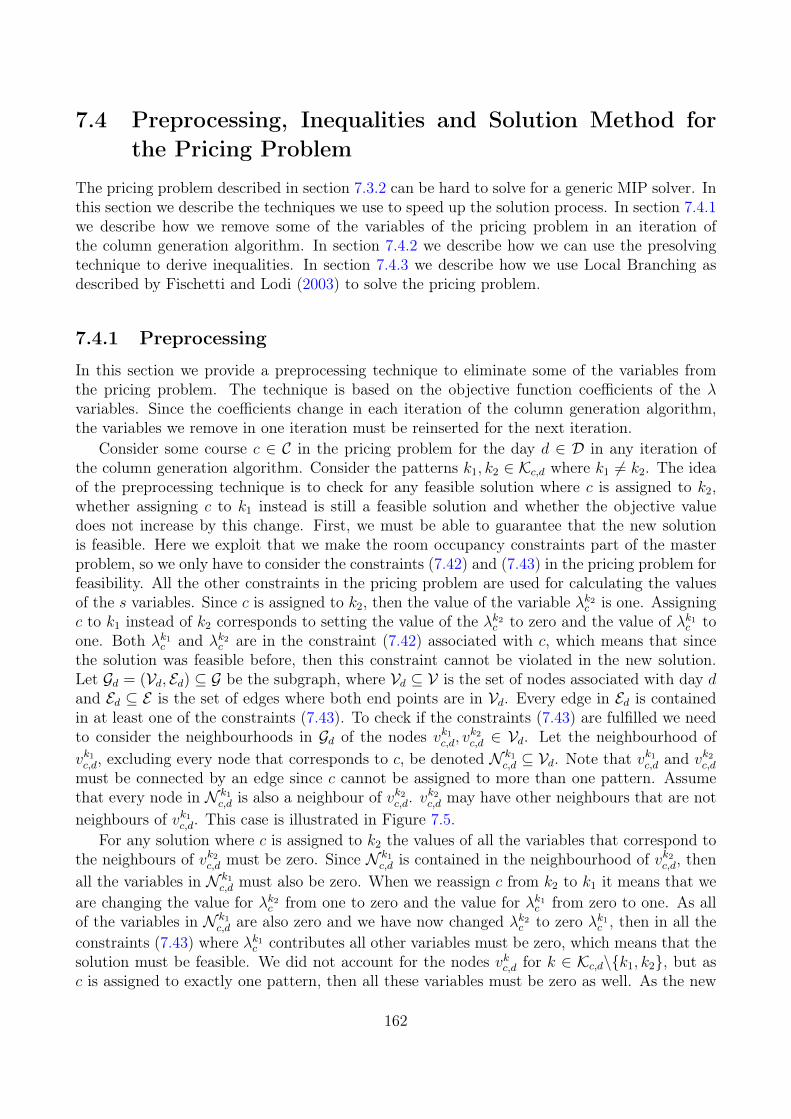
7.4 Preprocessing, Inequalities and Solution Method forthe Pricing Problem

The pricing problem described in section 7.3.2 can be hard to solve for a generic MIP solver. Inthis section we describe the techniques we use to speed up the solution process. In section 7.4.1we describe how we remove some of the variables of the pricing problem in an iteration ofthe column generation algorithm. In section 7.4.2 we describe how we can use the presolvingtechnique to derive inequalities. In section 7.4.3 we describe how we use Local Branching asdescribed by Fischetti and Lodi (2003) to solve the pricing problem.

7.4.1 Preprocessing

In this section we provide a preprocessing technique to eliminate some of the variables fromthe pricing problem. The technique is based on the objective function coefficients of the λvariables. Since the coefficients change in each iteration of the column generation algorithm,the variables we remove in one iteration must be reinserted for the next iteration.

Consider some course c ∈ C in the pricing problem for the day d ∈ D in any iteration ofthe column generation algorithm. Consider the patterns k1, k2 ∈ Kc,d where k1 6= k2. The ideaof the preprocessing technique is to check for any feasible solution where c is assigned to k2,whether assigning c to k1 instead is still a feasible solution and whether the objective valuedoes not increase by this change. First, we must be able to guarantee that the new solutionis feasible. Here we exploit that we make the room occupancy constraints part of the masterproblem, so we only have to consider the constraints (7.42) and (7.43) in the pricing problem forfeasibility. All the other constraints in the pricing problem are used for calculating the valuesof the s variables. Since c is assigned to k2, then the value of the variable λk2c is one. Assigningc to k1 instead of k2 corresponds to setting the value of the λk2c to zero and the value of λk1c toone. Both λk1c and λk2c are in the constraint (7.42) associated with c, which means that sincethe solution was feasible before, then this constraint cannot be violated in the new solution.Let Gd = (Vd, Ed) ⊆ G be the subgraph, where Vd ⊆ V is the set of nodes associated with day dand Ed ⊆ E is the set of edges where both end points are in Vd. Every edge in Ed is containedin at least one of the constraints (7.43). To check if the constraints (7.43) are fulfilled we needto consider the neighbourhoods in Gd of the nodes vk1c,d, v

k2c,d ∈ Vd. Let the neighbourhood of

vk1c,d, excluding every node that corresponds to c, be denoted N k1c,d ⊆ Vd. Note that vk1c,d and vk2c,d

must be connected by an edge since c cannot be assigned to more than one pattern. Assumethat every node in N k1

c,d is also a neighbour of vk2c,d. vk2c,d may have other neighbours that are not

neighbours of vk1c,d. This case is illustrated in Figure 7.5.For any solution where c is assigned to k2 the values of all the variables that correspond to

the neighbours of vk2c,d must be zero. Since N k1c,d is contained in the neighbourhood of vk2c,d, then

all the variables in N k1c,d must also be zero. When we reassign c from k2 to k1 it means that we

are changing the value for λk2c from one to zero and the value for λk1c from zero to one. As allof the variables in N k1

c,d are also zero and we have now changed λk2c to zero λk1c , then in all theconstraints (7.43) where λk1c contributes all other variables must be zero, which means that thesolution must be feasible. We did not account for the nodes vkc,d for k ∈ Kc,d\{k1, k2}, but asc is assigned to exactly one pattern, then all these variables must be zero as well. As the new

162

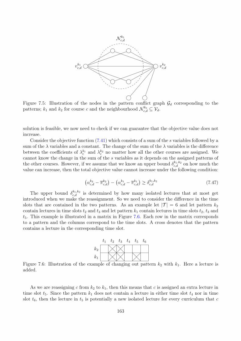
vk1c,d vk2c,d

N k1c,d

Figure 7.5: Illustration of the nodes in the pattern conflict graph Gd corresponding to thepatterns; k1 and k2 for course c and the neighbourhood N k1

c,d ⊆ Vd.

solution is feasible, we now need to check if we can guarantee that the objective value does notincrease.

Consider the objective function (7.41) which consists of a sum of the s variables followed by asum of the λ variables and a constant. The change of the sum of the λ variables is the differencebetween the coefficients of λk1c and λk2c no matter how all the other courses are assigned. Wecannot know the change in the sum of the s variables as it depends on the assigned patterns ofthe other courses. However, if we assume that we know an upper bound δk1,k2c,d on how much thevalue can increase, then the total objective value cannot increase under the following condition:(

αk2c,d − πk2c,d

)−(αk1c,d − π

k1c,d

)≥ δk1,k2c,d (7.47)

The upper bound δk1,k2c,d is determined by how many isolated lectures that at most getintroduced when we make the reassignment. So we need to consider the difference in the timeslots that are contained in the two patterns. As an example let |T | = 6 and let pattern k2

contain lectures in time slots t2 and t3 and let pattern k1 contain lectures in time slots t2, t3 andt5. This example is illustrated in a matrix in Figure 7.6. Each row in the matrix correspondsto a pattern and the columns correspond to the time slots. A cross denotes that the patterncontains a lecture in the corresponding time slot.

t1 t2 t3 t4 t5 t6

k2

k1

Figure 7.6: Illustration of the example of changing out pattern k2 with k1. Here a lecture isadded.

As we are reassigning c from k2 to k1, then this means that c is assigned an extra lecture intime slot t5. Since the pattern k1 does not contain a lecture in either time slot t4 nor in timeslot t6, then the lecture in t5 is potentially a new isolated lecture for every curriculum that c

163

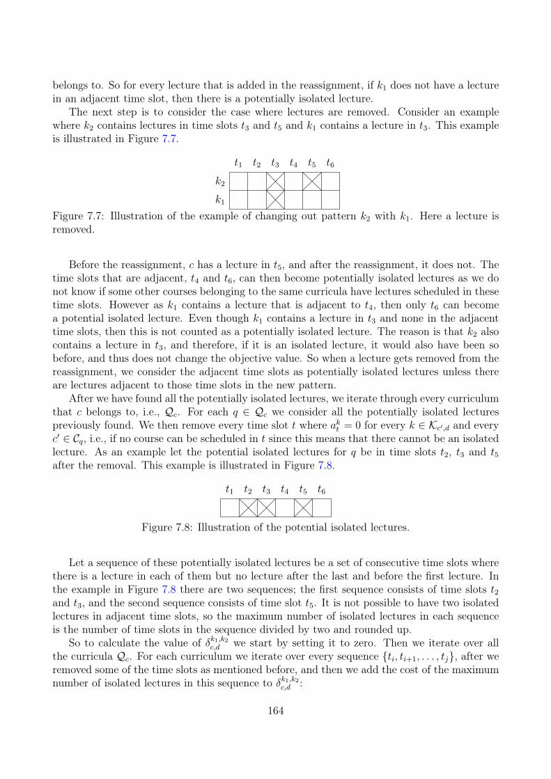
belongs to. So for every lecture that is added in the reassignment, if k1 does not have a lecturein an adjacent time slot, then there is a potentially isolated lecture.

The next step is to consider the case where lectures are removed. Consider an examplewhere k2 contains lectures in time slots t3 and t5 and k1 contains a lecture in t3. This exampleis illustrated in Figure 7.7.

t1 t2 t3 t4 t5 t6

k2

k1

Figure 7.7: Illustration of the example of changing out pattern k2 with k1. Here a lecture isremoved.

Before the reassignment, c has a lecture in t5, and after the reassignment, it does not. Thetime slots that are adjacent, t4 and t6, can then become potentially isolated lectures as we donot know if some other courses belonging to the same curricula have lectures scheduled in thesetime slots. However as k1 contains a lecture that is adjacent to t4, then only t6 can becomea potential isolated lecture. Even though k1 contains a lecture in t3 and none in the adjacenttime slots, then this is not counted as a potentially isolated lecture. The reason is that k2 alsocontains a lecture in t3, and therefore, if it is an isolated lecture, it would also have been sobefore, and thus does not change the objective value. So when a lecture gets removed from thereassignment, we consider the adjacent time slots as potentially isolated lectures unless thereare lectures adjacent to those time slots in the new pattern.

After we have found all the potentially isolated lectures, we iterate through every curriculumthat c belongs to, i.e., Qc. For each q ∈ Qc we consider all the potentially isolated lecturespreviously found. We then remove every time slot t where akt = 0 for every k ∈ Kc′,d and everyc′ ∈ Cq, i.e., if no course can be scheduled in t since this means that there cannot be an isolatedlecture. As an example let the potential isolated lectures for q be in time slots t2, t3 and t5after the removal. This example is illustrated in Figure 7.8.

t1 t2 t3 t4 t5 t6

Figure 7.8: Illustration of the potential isolated lectures.

Let a sequence of these potentially isolated lectures be a set of consecutive time slots wherethere is a lecture in each of them but no lecture after the last and before the first lecture. Inthe example in Figure 7.8 there are two sequences; the first sequence consists of time slots t2and t3, and the second sequence consists of time slot t5. It is not possible to have two isolatedlectures in adjacent time slots, so the maximum number of isolated lectures in each sequenceis the number of time slots in the sequence divided by two and rounded up.

So to calculate the value of δk1,k2c,d we start by setting it to zero. Then we iterate over allthe curricula Qc. For each curriculum we iterate over every sequence {ti, ti+1, . . . , tj}, after weremoved some of the time slots as mentioned before, and then we add the cost of the maximumnumber of isolated lectures in this sequence to δk1,k2c,d :

164

δk1,k2c,d ← δk1,k2c,d +W IL

⌈j − i+ 1

2

⌉(7.48)

Now we have calculated an upper bound on the increase in the cost of the isolated lectures.For a course c ∈ C and pattern k1, k2 ∈ Kc,d we say that k1 dominates k2 if (7.47) is fulfilled.If one pattern dominates another, then it implies that we can remove the dominated patternfrom the solution. However, we cannot remove all patterns that are dominated. As an example,consider a case where course c has five patterns; k1, k2, k3, k4 and k5. Assume that k1 dominatesk2, k2 dominates k3, k3 dominates k4, k4 dominates k5 and k5 dominates k1. This example isillustrated in Figure 7.9.

k1

k2

k3k4

k5

Figure 7.9: Illustration of five patterns of the example. The arrows illustrate the dominancebetween the patterns.

In the example, all the patterns are dominated so we could fix them all to zero. However,this would make the problem infeasible as c must select exactly one of them. So the way we dothe preprocessing is by considering one pattern k at a time, and if it is dominated by anotherpattern which is not fixed to zero, then we fix k to zero, i.e., we change the upper bound of thevariable from one to zero. In the example from Figure 7.9 we would for instance start with k5.Since k5 is dominated by k4 and k4 has not been fixed to zero, then we fix k5 to zero. We thengo to k4 which is dominated by k3, so we fix k3 to zero and so we continue until we get to k1.k1 is dominated by k5 but as k5 has already been fixed to zero we do not fix k1 to zero.

We apply the preprocessing technique described in this section before we solve the pricingproblem in every iteration of the column generation algorithm. When we have solved the pricingproblem we then unfix the variables again, i.e., we change the upper bounds of the variablesback to one, so they are ready for the next iteration.

7.4.2 Optimality Inequalities

In this section we describe an extension to the preprocessing technique from section 7.4.1.Like in the preprocessing phase, the inequalities we derive here are only applicable in a singleiteration of the column generation algorithm. Consider some course c ∈ C in the pricing problemfor a day d ∈ D in any iteration of the column generation algorithm. Consider the patternsk1, k2 ∈ Kc,d, where k1 6= k2. In section 7.4.1 we only considered the patterns k1 and k2 wherewe could guarantee that if we had a feasible solution where c was assigned to k2, then wecould create a new feasible solution by reassigning c to k1. In this section we do not keep thisrestriction, but consider every pair of patterns k1 and k2 where the condition (7.47) is fulfilled,i.e., where k1 dominates k2.

165

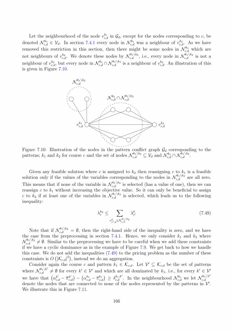
Let the neighbourhood of the node vk1c,d in Gd, except for the nodes corresponding to c, bedenoted N k1

c,d ∈ Vd. In section 7.4.1 every node in N k1c,d was a neighbour of vk2c,d. As we have

removed this restriction in this section, then there might be some nodes in N k1c,d which are

not neighbours of vk2c,d. We denote these nodes by N k1\k2c,d , i.e., every node in N k1\k2

c,d is not aneighbour of vk2c,d, but every node in N k1

c,d ∩Nk1\k2c,d is a neighbour of vk2c,d. An illustration of this

is given in Figure 7.10.

vk1c,d vk2c,d

N k1c,d ∩N

k1\k2c,d

N k1\k2c,d

Figure 7.10: Illustration of the nodes in the pattern conflict graph Gd corresponding to thepatterns; k1 and k2 for course c and the set of nodes N k1\k2

c,d ⊆ Vd and N k1c,d ∩N

k1\k2c,d .

Given any feasible solution where c is assigned to k2 then reassigning c to k1 is a feasiblesolution only if the values of the variables corresponding to the nodes in N k1\k2

c,d are all zero.This means that if none of the variable in N k1\k2

c,d is selected (has a value of one), then we canreassign c to k1 without increasing the objective value. So it can only be beneficial to assignc to k2 if at least one of the variables in N k1\k2

c,d is selected, which leads us to the followinginequality:

λk2c ≤∑

vkc′,d∈N

k1\k2c,d

λkc′ (7.49)

Note that if N k1\k2c,d = ∅, then the right-hand side of the inequality is zero, and we have

the case from the preprocessing in section 7.4.1. Hence, we only consider k1 and k2 whereN k1\k2c,d 6= ∅. Similar to the preprocessing we have to be careful when we add these constraints

if we have a cyclic dominance as in the example of Figure 7.9. We get back to how we handlethis case. We do not add the inequalities (7.49) to the pricing problem as the number of theseconstraints is O

(|Kc,d|2

), instead we do an aggregation.

Consider again the course c and pattern k1 ∈ Kc,d. Let V ′ ⊆ Kc,d be the set of patternswhere N k1\k′

c,d 6= ∅ for every k′ ∈ V ′ and which are all dominated by k1, i.e., for every k′ ∈ V ′

we have that(αk′

c,d − πk′

c,d

)−(αk1c,d − π

k1c,d

)≥ δk1,k

′

c,d . In the neighbourhood N k1c,d we let N k1\V ′

c,d

denote the nodes that are connected to none of the nodes represented by the patterns in V ′.We illustrate this in Figure 7.11.

166

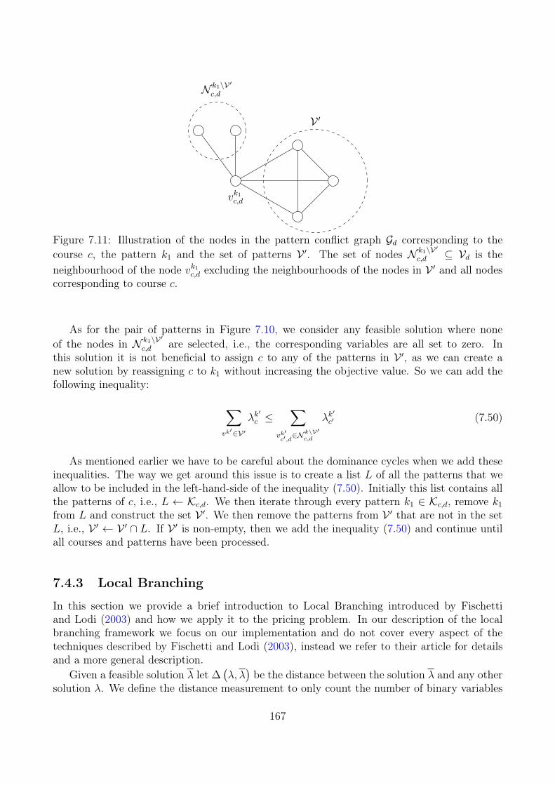
vk1c,d

V ′

N k1\V ′c,d

Figure 7.11: Illustration of the nodes in the pattern conflict graph Gd corresponding to thecourse c, the pattern k1 and the set of patterns V ′. The set of nodes N k1\V ′

c,d ⊆ Vd is theneighbourhood of the node vk1c,d excluding the neighbourhoods of the nodes in V ′ and all nodescorresponding to course c.

As for the pair of patterns in Figure 7.10, we consider any feasible solution where noneof the nodes in N k1\V ′

c,d are selected, i.e., the corresponding variables are all set to zero. Inthis solution it is not beneficial to assign c to any of the patterns in V ′, as we can create anew solution by reassigning c to k1 without increasing the objective value. So we can add thefollowing inequality:

∑vk′∈V ′

λk′

c ≤∑

vk′c′,d∈N

k\V′c,d

λk′

c′ (7.50)

As mentioned earlier we have to be careful about the dominance cycles when we add theseinequalities. The way we get around this issue is to create a list L of all the patterns that weallow to be included in the left-hand-side of the inequality (7.50). Initially this list contains allthe patterns of c, i.e., L ← Kc,d. We then iterate through every pattern k1 ∈ Kc,d, remove k1

from L and construct the set V ′. We then remove the patterns from V ′ that are not in the setL, i.e., V ′ ← V ′ ∩ L. If V ′ is non-empty, then we add the inequality (7.50) and continue untilall courses and patterns have been processed.

7.4.3 Local Branching

In this section we provide a brief introduction to Local Branching introduced by Fischettiand Lodi (2003) and how we apply it to the pricing problem. In our description of the localbranching framework we focus on our implementation and do not cover every aspect of thetechniques described by Fischetti and Lodi (2003), instead we refer to their article for detailsand a more general description.

Given a feasible solution λ let ∆(λ, λ)be the distance between the solution λ and any other

solution λ. We define the distance measurement to only count the number of binary variables

167

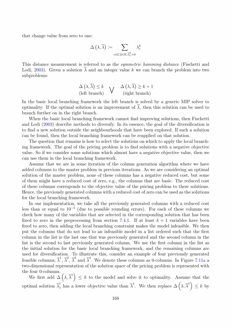
that change value from zero to one:

∆(λ, λ)

:=∑

c∈C,k∈K:λkc=0

λkc

This distance measurement is referred to as the symmetric hamming distance (Fischetti andLodi, 2003). Given a solution λ and an integer value k we can branch the problem into twosubproblems:

∆(λ, λ)≤ k

(left branch)

∨ ∆(λ, λ)≥ k + 1

(right branch)

In the basic local branching framework the left branch is solved by a generic MIP solver tooptimality. If the optimal solution is an improvement of λ, then this solution can be used tobranch further on in the right branch.

When the basic local branching framework cannot find improving solutions, then Fischettiand Lodi (2003) describe methods to diversify. In its essence, the goal of the diversification isto find a new solution outside the neighbourhoods that have been explored. If such a solutioncan be found, then the local branching framework can be reapplied on that solution.

The question that remains is how to select the solutions on which to apply the local branch-ing framework. The goal of the pricing problem is to find solutions with a negative objectivevalue. So if we consider some solutions which almost have a negative objective value, then wecan use them in the local branching framework.

Assume that we are in some iteration of the column generation algorithm where we haveadded columns to the master problem in previous iterations. As we are considering an optimalsolution of the master problem, none of these columns has a negative reduced cost, but someof them might have a reduced cost of zero, e.g., the columns that are basic. The reduced costof these columns corresponds to the objective value of the pricing problem to these solutions.Hence, the previously generated columns with a reduced cost of zero can be used as the solutionsfor the local branching framework.

In our implementation, we take all the previously generated columns with a reduced costless than or equal to 10−5 (due to possible rounding errors). For each of these columns wecheck how many of the variables that are selected in the corresponding solution that has beenfixed to zero in the preprocessing from section 7.4.1. If at least k + 1 variables have beenfixed to zero, then adding the local branching constraint makes the model infeasible. We thenput the columns that do not lead to an infeasible model in a list ordered such that the firstcolumn in the list is the last one that was previously generated and the second column in thelist is the second to last previously generated column. We use the first column in the list asthe initial solution for the basic local branching framework, and the remaining columns areused for diversification. To illustrate this, consider an example of four previously generatedfeasible columns; λ1, λ2, λ3 and λ4. We denote these columns as 0-columns. In Figure 7.11a atwo-dimensional representation of the solution space of the pricing problem is represented withthe four 0-columns.

We first add ∆(λ, λ

1)≤ k to the model and solve it to optimality. Assume that the

optimal solution λ1

1 has a lower objective value than λ1. We then replace ∆

(λ, λ

1)≤ k by

168

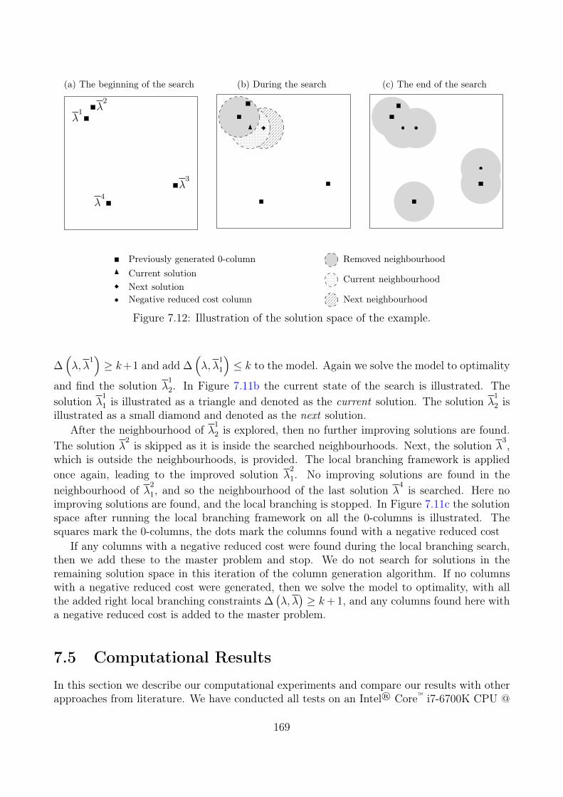
(a) The beginning of the search

λ1

λ2

λ3

λ4

(b) During the search (c) The end of the search

Previously generated 0-columnCurrent solutionNext solutionNegative reduced cost column

Removed neighbourhood

Current neighbourhood

Next neighbourhood

Figure 7.12: Illustration of the solution space of the example.

∆(λ, λ

1)≥ k+1 and add ∆

(λ, λ

1

1

)≤ k to the model. Again we solve the model to optimality

and find the solution λ1

2. In Figure 7.11b the current state of the search is illustrated. Thesolution λ1

1 is illustrated as a triangle and denoted as the current solution. The solution λ1

2 isillustrated as a small diamond and denoted as the next solution.

After the neighbourhood of λ1

2 is explored, then no further improving solutions are found.The solution λ2 is skipped as it is inside the searched neighbourhoods. Next, the solution λ3,which is outside the neighbourhoods, is provided. The local branching framework is appliedonce again, leading to the improved solution λ

2

1. No improving solutions are found in theneighbourhood of λ2

1, and so the neighbourhood of the last solution λ4 is searched. Here no

improving solutions are found, and the local branching is stopped. In Figure 7.11c the solutionspace after running the local branching framework on all the 0-columns is illustrated. Thesquares mark the 0-columns, the dots mark the columns found with a negative reduced cost

If any columns with a negative reduced cost were found during the local branching search,then we add these to the master problem and stop. We do not search for solutions in theremaining solution space in this iteration of the column generation algorithm. If no columnswith a negative reduced cost were generated, then we solve the model to optimality, with allthe added right local branching constraints ∆

(λ, λ)≥ k+ 1, and any columns found here with

a negative reduced cost is added to the master problem.

7.5 Computational Results

In this section we describe our computational experiments and compare our results with otherapproaches from literature. We have conducted all tests on an Intel® Core™ i7-6700K CPU @

169

4.00GHz processor with four cores and eight logical processors and 32GB memory, running Win-dows 10. We use Gurobi version 7.0.1 provided by Gurobi Optimization, Inc. (2016) both for themaster problem and in the pricing problems. We set the presolver to the most aggressive set-ting (Presolve=2), the number of threads to be equal to the number of processors (Threads=8)and the MIP gap to zero (MIPGap=0.0). The cut-off value is set to −10−5 (CUTOFF=-1e-5), such that the solver will not return solutions with objective values which are greater than−10−5. We set the limit on the solutions to be returned to be the maximum possible (Solution-Limit=int.MaxValue) so we can extract all the columns that Gurobi generates with a negativereduced cost. The remaining parameters are set to their default value. We have implementedour code in C#, and we use the Parallel.ForEach method from the System.Threading.Taskslibrary to solve the pricing problems in parallel as they are independent.

We test our algorithm on 20 of the 21 data instances from ITC2007 named comp01 throughcomp21. The data instance that we do not include in the tests is comp11. The reason fornot including this instance is the same reason that Cacchiani et al. (2013) do not include thisinstance in their tests, which is that the best-known upper bound is zero, and so we cannotimprove the trivial lower bound of zero.

As the pricing problems that we solve are the same, except for the objective function, ineach iteration, we build the model in Gurobi once and then change the objective functionaccordingly in each iteration. All the variables that are removed in the preprocessing phasedescribed in section 7.4.1 are not removed from the model, but the upper bounds are set to zeroinstead. After the preprocessing the inequalities from section 7.4.2 are added, and then thelocal branching framework is provided with the model. All the calculations for the potentiallyisolated lectures in section 7.4.1 and 7.4.2 are performed when the pricing problems are builtand the information is stored in a table so that we do not have to recalculate these values.We retrieve every column found by Gurobi that has a negative reduced cost and add them tothe master problem. Afterwards, we remove all the constraints that we added in the pricingproblems and set the upper bounds back to one.

We need to decide the value for k in the local branching framework. Fischetti and Lodi(2003) suggest to set it between 10 and 20, which in our case is between 5 and 10, as weare using the symmetric hamming distance. So we have tested the algorithm for k = 5 andk = 10. Furthermore, we have also tested for k = 2. The reason for testing for k = 2 is tomimic a 2-exchange heuristic (Wolsey, 1998). The total running time, including the time ofbuilding the model, the preprocessing and the enumeration of cliques, is reported in Table 7.2for k ∈ {2, 5, 10}. The timings are reported in the format hh:mm:ss where hh is the amount ofhours, mm is the amount of minutes and ss is the seconds. In the line (Total) the total amountof time spent is reported for each value of k and (Best) counts the number of times each valueof k has the lowest running time.

In Table 7.2 we see that the algorithm is fastest for k = 2 regarding the total time to solveall instances. In the table we also see that in 13 out of the 20 instances the setting k = 2 isfaster than for the other values. Thus, in the subsequent tests we report the results for k = 2.

In Table 7.3 we report the statistics of the column generation algorithm. For each data in-stance we report the number of iterations (Iter.). Then in the two following columns (Columns),we report the number of columns that were generated in total (Total) and how many of themthat where generated by local branching (LocBra.). In the next four columns (Time) we reportthe timings of the algorithm. The total time spent by the algorithm is reported in the column

170

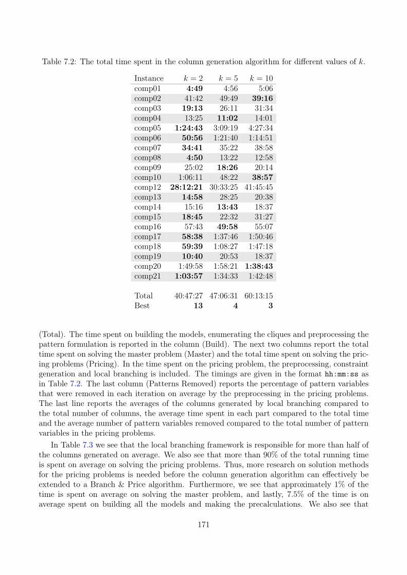
Table 7.2: The total time spent in the column generation algorithm for different values of k.

Instance k = 2 k = 5 k = 10comp01 4:49 4:56 5:06comp02 41:42 49:49 39:16comp03 19:13 26:11 31:34comp04 13:25 11:02 14:01comp05 1:24:43 3:09:19 4:27:34comp06 50:56 1:21:40 1:14:51comp07 34:41 35:22 38:58comp08 4:50 13:22 12:58comp09 25:02 18:26 20:14comp10 1:06:11 48:22 38:57comp12 28:12:21 30:33:25 41:45:45comp13 14:58 28:25 20:38comp14 15:16 13:43 18:37comp15 18:45 22:32 31:27comp16 57:43 49:58 55:07comp17 58:38 1:37:46 1:50:46comp18 59:39 1:08:27 1:47:18comp19 10:40 20:53 18:37comp20 1:49:58 1:58:21 1:38:43comp21 1:03:57 1:34:33 1:42:48

Total 40:47:27 47:06:31 60:13:15Best 13 4 3

(Total). The time spent on building the models, enumerating the cliques and preprocessing thepattern formulation is reported in the column (Build). The next two columns report the totaltime spent on solving the master problem (Master) and the total time spent on solving the pric-ing problems (Pricing). In the time spent on the pricing problem, the preprocessing, constraintgeneration and local branching is included. The timings are given in the format hh:mm:ss asin Table 7.2. The last column (Patterns Removed) reports the percentage of pattern variablesthat were removed in each iteration on average by the preprocessing in the pricing problems.The last line reports the averages of the columns generated by local branching compared tothe total number of columns, the average time spent in each part compared to the total timeand the average number of pattern variables removed compared to the total number of patternvariables in the pricing problems.

In Table 7.3 we see that the local branching framework is responsible for more than half ofthe columns generated on average. We also see that more than 90% of the total running timeis spent on average on solving the pricing problems. Thus, more research on solution methodsfor the pricing problems is needed before the column generation algorithm can effectively beextended to a Branch & Price algorithm. Furthermore, we see that approximately 1% of thetime is spent on average on solving the master problem, and lastly, 7.5% of the time is onaverage spent on building all the models and making the precalculations. We also see that

171

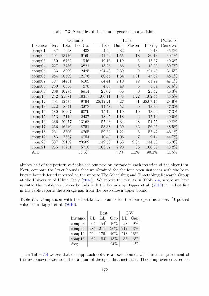
Table 7.3: Statistics of the column generation algorithm.

Columns Time PatternsInstance Iter. Total LocBra. Total Build Master Pricing Removedcomp01 37 1058 433 4:49 2:32 0 2:13 45.8%comp02 191 13776 9160 41:42 1:55 18 39:13 40.1%comp03 150 6762 1946 19:13 1:19 5 17:37 40.3%comp04 227 7786 3821 13:25 56 8 12:03 50.7%comp05 133 3909 2425 1:24:43 2:39 2 1:21:43 31.5%comp06 284 20509 12076 50:56 1:34 1:01 47:52 48.1%comp07 197 14451 6109 34:41 2:10 42 31:24 47.1%comp08 239 6038 870 4:50 49 8 3:34 51.5%comp09 208 10274 6914 25:02 56 9 23:42 46.3%comp10 252 25381 18317 1:06:11 1:36 1:22 1:02:44 46.5%comp12 301 12474 9794 28:12:21 3:27 31 28:07:14 28.6%comp13 222 8641 3273 14:58 52 9 13:39 47.3%comp14 180 10067 6079 15:16 1:10 10 13:40 47.3%comp15 153 7119 2437 18:45 1:18 6 17:10 40.0%comp16 236 20077 13168 57:43 1:34 48 54:55 49.8%comp17 266 16640 8751 58:38 1:29 36 56:05 48.5%comp18 231 5606 4205 59:39 1:22 5 57:42 46.1%comp19 183 7857 4054 10:40 1:06 7 9:14 44.7%comp20 307 32159 23802 1:49:58 1:55 2:34 1:44:50 46.3%comp21 285 15251 5710 1:03:57 2:20 36 1:00:33 43.2%Avg. 53.5% 7.5% 1.1% 90.1% 44.5%

almost half of the pattern variables are removed on average in each iteration of the algorithm.Next, compare the lower bounds that we obtained for the four open instances with the best-known bounds found reported on the website The Scheduling and Timetabling Research Groupat the University of Udine, Italy (2015). We report the results in Table 7.4, where we haveupdated the best-known lower bounds with the bounds by Bagger et al. (2016). The last linein the table reports the average gap from the best-known upper bound.

Table 7.4: Comparison with the best-known bounds for the four open instances. *Updatedvalue from Bagger et al. (2016).

Best DWInstance UB LB Gap LB Gapcomp03 64 54* 16% 58 9%comp05 284 211 26% 247 13%comp12 294 175* 40% 248 16%comp15 62 54* 13% 58 6%Avg. 24% 11%

In Table 7.4 we see that our approach obtains a lower bound, which is an improvement ofthe best-known lower bound for all four of the open data instances. These improvements reduce

172

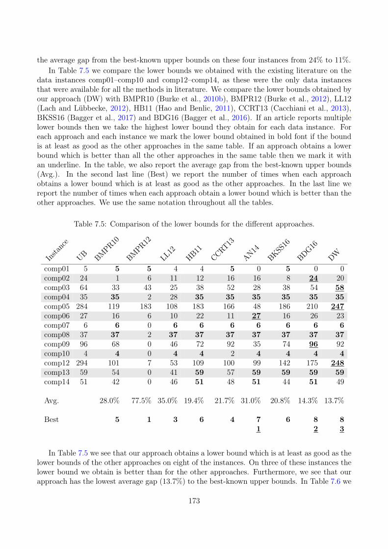
the average gap from the best-known upper bounds on these four instances from 24% to 11%.In Table 7.5 we compare the lower bounds we obtained with the existing literature on the

data instances comp01–comp10 and comp12–comp14, as these were the only data instancesthat were available for all the methods in literature. We compare the lower bounds obtained byour approach (DW) with BMPR10 (Burke et al., 2010b), BMPR12 (Burke et al., 2012), LL12(Lach and Lübbecke, 2012), HB11 (Hao and Benlic, 2011), CCRT13 (Cacchiani et al., 2013),BKSS16 (Bagger et al., 2017) and BDG16 (Bagger et al., 2016). If an article reports multiplelower bounds then we take the highest lower bound they obtain for each data instance. Foreach approach and each instance we mark the lower bound obtained in bold font if the boundis at least as good as the other approaches in the same table. If an approach obtains a lowerbound which is better than all the other approaches in the same table then we mark it withan underline. In the table, we also report the average gap from the best-known upper bounds(Avg.). In the second last line (Best) we report the number of times when each approachobtains a lower bound which is at least as good as the other approaches. In the last line wereport the number of times when each approach obtain a lower bound which is better than theother approaches. We use the same notation throughout all the tables.

Table 7.5: Comparison of the lower bounds for the different approaches.

Instance

UB BMPR

10

BMPR

12

LL12

HB11

CCRT13

AN14

BKSS16

BDG16

DW

comp01 5 5 5 4 4 5 0 5 0 0comp02 24 1 6 11 12 16 16 8 24 20comp03 64 33 43 25 38 52 28 38 54 58comp04 35 35 2 28 35 35 35 35 35 35comp05 284 119 183 108 183 166 48 186 210 247comp06 27 16 6 10 22 11 27 16 26 23comp07 6 6 0 6 6 6 6 6 6 6comp08 37 37 2 37 37 37 37 37 37 37comp09 96 68 0 46 72 92 35 74 96 92comp10 4 4 0 4 4 2 4 4 4 4comp12 294 101 7 53 109 100 99 142 175 248comp13 59 54 0 41 59 57 59 59 59 59comp14 51 42 0 46 51 48 51 44 51 49

Avg. 28.0% 77.5% 35.0% 19.4% 21.7% 31.0% 20.8% 14.3% 13.7%

Best 5 1 3 6 4 7 6 8 81 2 3

In Table 7.5 we see that our approach obtains a lower bound which is at least as good as thelower bounds of the other approaches on eight of the instances. On three of these instances thelower bound we obtain is better than for the other approaches. Furthermore, we see that ourapproach has the lowest average gap (13.7%) to the best-known upper bounds. In Table 7.6 we

173

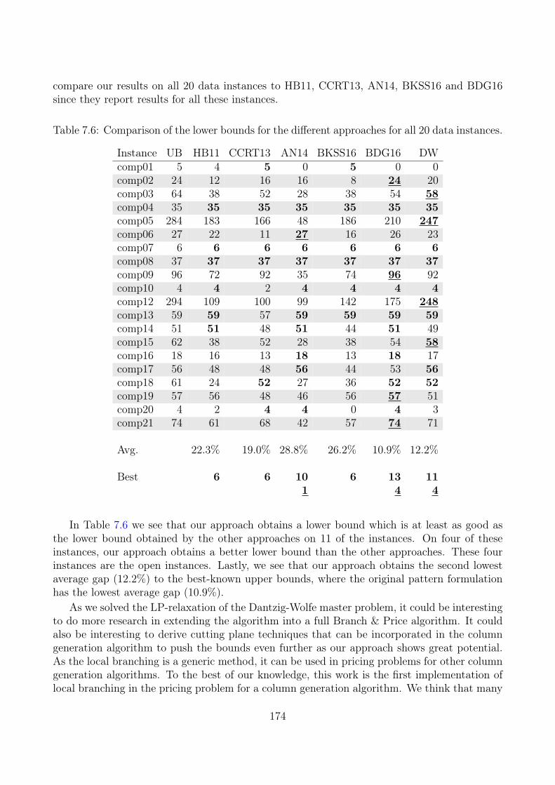
compare our results on all 20 data instances to HB11, CCRT13, AN14, BKSS16 and BDG16since they report results for all these instances.

Table 7.6: Comparison of the lower bounds for the different approaches for all 20 data instances.

Instance UB HB11 CCRT13 AN14 BKSS16 BDG16 DWcomp01 5 4 5 0 5 0 0comp02 24 12 16 16 8 24 20comp03 64 38 52 28 38 54 58comp04 35 35 35 35 35 35 35comp05 284 183 166 48 186 210 247comp06 27 22 11 27 16 26 23comp07 6 6 6 6 6 6 6comp08 37 37 37 37 37 37 37comp09 96 72 92 35 74 96 92comp10 4 4 2 4 4 4 4comp12 294 109 100 99 142 175 248comp13 59 59 57 59 59 59 59comp14 51 51 48 51 44 51 49comp15 62 38 52 28 38 54 58comp16 18 16 13 18 13 18 17comp17 56 48 48 56 44 53 56comp18 61 24 52 27 36 52 52comp19 57 56 48 46 56 57 51comp20 4 2 4 4 0 4 3comp21 74 61 68 42 57 74 71

Avg. 22.3% 19.0% 28.8% 26.2% 10.9% 12.2%

Best 6 6 10 6 13 111 4 4

In Table 7.6 we see that our approach obtains a lower bound which is at least as good asthe lower bound obtained by the other approaches on 11 of the instances. On four of theseinstances, our approach obtains a better lower bound than the other approaches. These fourinstances are the open instances. Lastly, we see that our approach obtains the second lowestaverage gap (12.2%) to the best-known upper bounds, where the original pattern formulationhas the lowest average gap (10.9%).

As we solved the LP-relaxation of the Dantzig-Wolfe master problem, it could be interestingto do more research in extending the algorithm into a full Branch & Price algorithm. It couldalso be interesting to derive cutting plane techniques that can be incorporated in the columngeneration algorithm to push the bounds even further as our approach shows great potential.As the local branching is a generic method, it can be used in pricing problems for other columngeneration algorithms. To the best of our knowledge, this work is the first implementation oflocal branching in the pricing problem for a column generation algorithm. We think that many

174

pricing problems, in general, fits well with local branching since every iteration of the columngeneration algorithm provides new solutions to be used in the framework.

7.6 ConclusionIn this article we applied a Dantzig-Wolfe Decomposition on a pattern formulation for theCurriculum-based Course Timetabling problem. The pattern formulation is based on enu-merating all the time schedules to which the courses can be assigned each day. The patternformulation only considers the time schedule of the problem. Thus, the formulation is a lowerbounding method for the original problem. The decomposition resulted in a pricing problemfor each day, where each pricing problem generates a schedule for an entire day. We showedthat the pricing problem contained a special structure which we exploited in a preprocessingphase. We then showed how the preprocessing technique could be used to derive inequalitiesfor the pricing problem. Lastly, we described how we applied Local Branching to solve thepricing problem. To the best of our knowledge, this is the first time Local Branching is imple-mented in a pricing problem, but it is general enough to be applied in other column generationalgorithms. We tested our algorithm on 20 data instances used in the second InternationalTimetabling Competition. On these instances the preprocessing technique we applied removedmore than 40% of the pattern variables from the pricing problem on average. We compared thelower bounds that we obtained with other approaches from literature. In 11 of the instancesour algorithm obtained a lower bound which was at least as good as the other approaches. Fourof these instances are still open, meaning that the best-known upper bound does not equal thebest-known lower bound. In all of these four instances our algorithm improved the lower bound,such that the average gap was decreased from 24% to 11%. We showed that more than 90% ofthe total time of the algorithm were spent on solving the pricing problem, and we concludedthat more research is needed in the pricing problems before the algorithm is extended into afull Branch & Price Algorithm.

AcknowledgmentsThe authors would like to thank Guy Desaulniers and Jacques Desrosiers for their contributionto the previous work on which this paper is based. The authors would also like to thankChristina Scheel Persson for her valuable feedback to improve the manuscript.

Funding: This work is part of an industrial PhD project funded by Innovation Fund Den-mark (IFD). IFD has supported this work solely financially and has not taken part in anyresearch related activities.

ReferencesAsín Aschá, R. and Nieuwenhuis, R. (2014). “Curriculum-based course timetabling with SAT

and MaxSAT”. In: Annals of Operations Research 218, pp. 71–91.

175

Bagger, N.-C. F., Kristiansen, S., Sørensen, M., and Stidsen, T. R. (2017). “Flow Formulationsfor Curriculum-based Course Timetabling”. In: Submitted to Annals of Operations Research.Preprint available at Optimization-Online.org. url: http://www.optimization-online.org/DB_HTML/2016/12/5786.html.

Bagger, N.-C. F., Desaulniers, G., and Desrosiers, J. (2016). “Daily course pattern formulationand valid inequalities for the curriculum-based course timetabling problem”. In: Submittedto Journal of Scheduling. Preprint available from Les Cahiers du GERAD. url: https://www.gerad.ca/en/papers/G-2016-71.

Bettinelli, A., Cacchiani, V., Roberti, R., and Toth, P. (2015). “An overview of curriculum-basedcourse timetabling”. In: TOP 23.2, pp. 313–349.

Bonutti, A., De Cesco, F., Di Gaspero, L., and Schaerf, A. (2012). “Benchmarking curriculum-based course timetabling: Formulations, data formats, instances, validation, visualization,and results”. In: Annals of Operations Research 194.1, pp. 59–70.

Bron, C. and Kerbosch, J. (1973). “Algorithm 457: Finding All Cliques of an Undirected Graph”.In: Communications of the ACM 16.9, pp. 575–577. doi: 10.1145/362342.362367. url:http://doi.acm.org/10.1145/362342.362367.

Burke, E. K., Mareček, J., Parkes, A. J., and Rudová, H. (2008). “Penalising Patterns in Timeta-bles: Novel Integer Programming Formulations”. In: Operations Research Proceedings 2007.Springer, pp. 409–414.

Burke, E. K., Mareček, J., Parkes, A. J., and Rudová, H. (2010a). “A supernodal formulation ofvertex colouring with applications in course timetabling”. In: Annals of Operations Research179.1, pp. 105–130.

Burke, E. K., Mareček, J., Parkes, A. J., and Rudová, H. (2010b). “Decomposition, reformu-lation, and diving in university course timetabling”. In: Computers & Operations Research37.3, pp. 582–597. doi: 10.1016/j.cor.2009.02.023.

Burke, E. K., Mareček, J., Parkes, A. J., and Rudová, H. (2012). “A branch-and-cut proce-dure for the Udine Course Timetabling problem”. In: Annals of Operations Research 194.1,pp. 71–87.

Cacchiani, V., Caprara, A., Roberti, R., and Toth, P. (2013). “A new lower bound for curriculum-based course timetabling”. In: Computers and Operation Research 40.10, pp. 2466–2477. doi:10.1016/j.cor.2013.02.010.

Desrosiers, J. and Lübbecke, M. E. (2010). “A Primer in Column Generation”. In: ColumnGeneration. Ed. by Guy Desaulniers, Jacques Desrosiers, and Marius M. Solomon. SpringerScience+Business Media, Inc. Chap. 1, pp. 1–32. isbn: 978-1-4419-3799-5.

Di Gaspero, L., Schaerf, A., and McCollum, B. (2007). “The Second International TimetablingCompetition (ITC-2007): Curriculum-based Course Timetabling (Track 3) — preliminarypresentation—”. In:Association for the Advancement of Artificial Intelligence (www.aaai.org).

Fischetti, M. and Lodi, A. (2003). “Local branching”. In: Mathematical Programming 98.1-3,pp. 23–47. doi: 10.1007/s10107-003-0395-5.

Gurobi Optimization, Inc. (2016). Gurobi Optimizer Reference Manual. url: http://www.gurobi.com.

Hao, J. K. and Benlic, U. (2011). “Lower bounds for the ITC-2007 curriculum-based coursetimetabling problem”. In: European Journal of Operational Research 212.3, pp. 464–472.

176

Lach, G. and Lübbecke, M. E. (2008). “Optimal University Course Timetables and the Par-tial Transversal Polytope”. In: International Workshop on Experimental and Efficient Algo-rithms. Springer, pp. 235–248.

Lach, G. and Lübbecke, M. E. (2012). “Curriculum based course timetabling: New solutions toUdine benchmark instances”. In: Annals of Operations Research 194.1, pp. 255–272.

Lübbecke, M. E. (2015). “Comments on: An Overview of Curriculum-Based Course Timetabling”.In: TOP 23.2, pp. 359–361.

Martin, R. K. (1999). Large scale linear and integer optimization: a unified approach. KluwerAcademic Publishers.

McCollum, B., Schaerf, A., Paechter, B., McMullan, P., Lewis, R., Parkes, A. J., Di Gaspero,L., Qu, R., and Burke, E. K. (2010). “Setting the research agenda in automated timetabling:The second international timetabling competition”. In: INFORMS Journal on Computing22.1, pp. 120–130.

The Scheduling and Timetabling Research Group at the University of Udine, Italy (2015).Curriculum-Based Course TimeTabling. Last retrieved October 2015, http://tabu.diegm.uniud.it/ctt/index.php. url: http://tabu.diegm.uniud.it/ctt/index.php.

Wolsey, L. A. (1998). “Heuristic Algorithms”. In: Integer Programming. Ed. by R. L. Graham,J. K. Lenstra, and R. E. Tarjan. John Wiley & Sons, Inc. Chap. 12, pp. 203–220. isbn:0-471-28366-5.

177