Mathematical Optimization Approaches for FacilityLayout Problems: The State-of-the-Art and Future

Research Directions

Miguel F. Anjosa,1, Manuel V.C. Vieirab,2

aGERAD & Department of Mathematics and Industrial Engineering, PolytechniqueMontreal, Canada

bDepartamento de Matematica, Faculdade de Ciencias e Tecnologia & CMA,Universidade Nova de Lisboa, Portugal

Abstract

Facility layout problems are an important class of operations research prob-lems that has been studied for several decades. Most variants of facility lay-out are NP-hard, therefore global optimal solutions are difficult or impossibleto compute in reasonable time. Mathematical optimization approaches thatguarantee global optimality of solutions or tight bounds on the global opti-mal value have nevertheless been successfully applied to several variants offacility layout. This review covers three classes of layout problems, namelyrow layout, unequal-areas layout, and multifloor layout. We summarizethe main contributions to the area made using mathematical optimization,mostly mixed integer linear optimization and conic optimization. For eachclass of problems, we also briefly discuss directions that remain open forfuture research.

Keywords: Facilities planning and design, unequal-areas facility layout,row layout, mixed integer linear optimization, semidefinite optimization.

Email addresses: anjos@stanfordalumni.org (Miguel F. Anjos), mvcv@fct.unl.pt(Manuel V.C. Vieira)

URL: http://www.miguelanjos.com (Miguel F. Anjos)1This author’s research was partially supported by the Natural Sciences and Engineer-

ing Research Council of Canada.2This author’s research was partially supported by the Fundacao para a Ciencia e

a Tecnologia (Portuguese Foundation for Science and Technology) through the projectPEstOE/MAT/UI0297/2014 (Centro de Matematica e Aplicacoes).

Preprint submitted to Elsevier January 26, 2017

1. Introduction

Facility layout problems (FLPs) are a general class of operations researchproblems concerned with finding the optimal arrangement of a given num-ber of nonoverlapping indivisible departments within a given facility. Theobjective is to minimize the total expected cost of inter-departmental flowsinside the facility, where the cost incurred for each pair of departments isequal to the rectilinear distance between the centroids of the departmentsmultiplied by their pairwise cost. This cost, generally non-negative, ac-counts in the aggregate for adjacency preferences as well as costs that mayarise from transportation, the construction of a material-handling system,or connection wiring. The facility and the departments are rectangular, andthe area of each department is specified, but if the department’s dimensionscan vary, then determining them is also part of the FLP.

FLPs have a variety of applications. Much of the work was motivatedby the physical organization of manufacturing systems, see e.g. [71]. TheFLP is particularly relevant in flexible manufacturing systems that producean array of different parts. The layout of the production components hasa significant impact on the costs and the productivity of these systems, seee.g. [39]. Other applications of FLPs include balancing hydraulic turbinerunners [60], algorithm initialization in numerical analysis [26], VLSI fixed-outline floorplanning [66], and optimal data memory layout generation fordigital signal processors [95].

FLPs have been extensively studied in the literature since the 1960s.Numerous variations on the basic problem described above have been con-sidered, and different models have been proposed for each variation. Ex-amples of such variations are: specially structured instances of the problem(e.g. layouts on rows or on loops); dynamic FLPs with time-dependencies;FLPs under uncertainty in the data; and multi-objective FLPs. We refer thereader to the books [59, 41] and survey papers [71, 91] for more informationabout the FLP and its variations. A growing collection of FLP benchmarkinstances is available online [14].

The FLP is NP-hard in general, so solving it to global optimality inreasonable time is generally difficult. Indeed the restricted version where thedimensions of the departments are all equal and fixed, and the optimizationis taken over a fixed set of possible locations for the departments, is knownas the quadratic assignment problem, a combinatorial optimization problemwell known for its computational difficulty, see e.g. [64].

The constraints of the basic FLP can be grouped into two sets:

• Department shape requirements include the required area, and restric-

2

tions on the dimensions (height and width) such as bounds on theratios height/width and width/height, called aspect ratios. These re-quirements generally lead to convex constraints but still pose somechallenges. In particular, requiring small aspect ratios, while desir-able in real-world applications, generally makes the problem harder.On the other hand, while the area constraint traditionally required acareful linearization approach, it can be modeled exactly using conicoptimization, see e.g. [18].

• Department location requirements include the nonoverlap of depart-ments, fitting every department within the facility, assigning certaindepartments to, or forbidding them from, particular locations withinthe facility. The main challenge here are the nonoverlap constraintsthat are inherently nonconvex and combinatorial.

This review is focused on FLPs with the following properties:

1. the departments have different areas

2. the facility can be one-, two-, or three-dimensional.

The different dimensions lead to the three broad classes of FLPs covered inthis review, namely row FLPs (Section 2), unequal-areas FLPs (Section 3),and multifloor FLPs (Section 4).

One-dimensional facilities lead to row FLPs, and we categorize them interms of the number of rows: single-row, double-row, or multi-row. Single-row and double-row problems commonly occur in practical applications, aswe discuss in Sections 2.1 and 2.2 respectively. Multi-row problems are anatural extension of the problem to three or more rows, and are consideredin Section 2.3.

Unequal-areas FLPs have two-dimensional facilities with a single floor,and we assume that the facility is rectangular and that all the departmentsfit inside the facility. Unlike in the case of row layouts, not only the positionbut also the dimensions of each department are optimized. After discussingmodels and approaches for the basic two-dimensional problem in Sections3.1 to 3.4, we consider in Section 3.5 the special case of flexible bay layouts, atype of layout that resembles row FLPs but with the fundamental differencethat the width of the bays can vary, depending on the total area of thedepartments in each bay.

Three-dimensional facilities give rise to multifloor FLPs in which depart-ments are to be placed over two or more floors. This is the focus of Section 4.The survey in Section 4.1 shows that this is a problem for which most of theliterature proposes models that are designed for specific applications rather

3

than for the general problem. For this reason we propose in Section 4.2 aformulation for a generic form of the problem that we hope will motivatefurther research into multifloor FLP.

Regarding the choice of methodologies, we limit the scope of this re-view to mathematical optimization-based approaches. These include exactmethods, but as the problems increase in difficulty very rapidly, we also in-clude heuristic methods that use mathematical optimization approximationsand/or relaxations. While there is a rich literature on heuristic algorithmsfor FLPs (see e.g. [71], [91], [57]), our focus here is on mathematical opti-mization approaches, primarily mixed integer linear optimization (MILO),often refereed to as mixed integer programming or MIP, semidefinite op-timization (SDO), also called semidefinite programming or SDP, and non-linear optimization. Because of their importance to the success of theseapproaches, we also include brief discussions of symmetry breaking (Section5) and valid inequalities (Section 6) as these are essential ingredients forsolving the resulting relaxations efficiently.

We conclude with a summary of directions for future research in Section7.

2. Row FLPs

Row FLPs share the following common problem statement: Given a setof rectangular departments each of a given length, a number of rows, and apairwise non-negative weight for each pair of departments, determine (i) anassignment of departments to rows, and (ii) the positions of the departmentsin each row, so that the total of the weighted center-to-center distances isminimized. Row FLPs arise in practical contexts where the departmentsare to be placed in rows with a predetermined separation between the rowsdue to factors such as the material-handling system or the flows of people.Moreover, within each row, a minimum clearance between departments isneeded to satisfy safety and operational requirements. We assume that thisclearance is included in the lengths of the departments. We also assume thatthe rows and the departments all have the same height, that any departmentcan be assigned to any row, and that the distances between adjacent rowsare equal. Under these assumptions, solving an instance of the row FLPmeans resolving three questions:

1. Assign each department to exactly one row;

2. Express mathematically the center-to-center distance between depart-ments (that may or may not be in the same row);

4

3. Handle possible empty space between departments.

Section 2.1 is concerned with the simplest version of row FLP, namelythe single-row FLP. Section 2.2 covers the double-row FLP, and Section 2.3extends the coverage to the general multirow FLP.

2.1. The Single-Row FLP

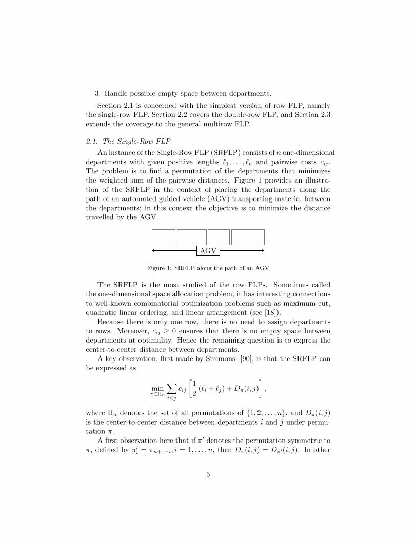
An instance of the Single-Row FLP (SRFLP) consists of n one-dimensionaldepartments with given positive lengths `1, . . . , `n and pairwise costs cij .The problem is to find a permutation of the departments that minimizesthe weighted sum of the pairwise distances. Figure 1 provides an illustra-tion of the SRFLP in the context of placing the departments along thepath of an automated guided vehicle (AGV) transporting material betweenthe departments; in this context the objective is to minimize the distancetravelled by the AGV.

AGV

Figure 1: SRFLP along the path of an AGV

The SRFLP is the most studied of the row FLPs. Sometimes calledthe one-dimensional space allocation problem, it has interesting connectionsto well-known combinatorial optimization problems such as maximum-cut,quadratic linear ordering, and linear arrangement (see [18]).

Because there is only one row, there is no need to assign departmentsto rows. Moreover, cij ≥ 0 ensures that there is no empty space betweendepartments at optimality. Hence the remaining question is to express thecenter-to-center distance between departments.

A key observation, first made by Simmons [90], is that the SRFLP canbe expressed as

minπ∈Πn

∑i<j

cij

[1

2(`i + `j) +Dπ(i, j)

],

where Πn denotes the set of all permutations of {1, 2, . . . , n}, and Dπ(i, j)is the center-to-center distance between departments i and j under permu-tation π.

A first observation here that if π′ denotes the permutation symmetric toπ, defined by π′i = πn+1−i, i = 1, . . . , n, then Dπ(i, j) = Dπ′(i, j). In other

5

words, the order of the departments in a particular layout can be reversedwithout changing the value of the objective function. Hence, it is possibleto simplify the problem by considering only the permutations that have aparticular facility, say facility 1, in the left half of the arrangement. Alterna-tively, we can require that a specific facility be to the left of another; this isknown as the position p− k method, see Section 5. This type of symmetry-breaking strategy can help reduce the computational cost of a mathematicaloptimization algorithm for SRFLP and for other types of layout problems,see Section 5. One aspect unique to the SDO-based approach is that it im-plicitly accounts for these symmetries, and thus does not require the use ofadditional explicit symmetry-breaking constraints, see Section 2.1.2.

A second observation is that it is not necessary to know the positionof each department; it suffices to know for each pair of departments whichdepartments are between them. Hence the key here is the concept of be-tweenness.

There is a large amount of literature on the SRFLP. For more detailed ex-positions on the state-of-the-art for the SRFLP, including extensions, meta-heuristics, and exact approaches, we refer the reader to [57] and to the recentreview paper [54] in this journal.

To give the reader a sense of the mathematical optimization approachesto the SRFLP, we present here two different ways to model betweenness.One is based on MILO and the other based on SDO.

2.1.1. MILO Model

The approach sketched here was originally proposed in [5]. Other MILOmodels for SRFLP include, in chronological order, [65], [43], [3], and [4].

For three distinct departments i, j, k, define the betweenness variablesζijk as:

ζijk =

{1, if department k lies between departments i and j,0, otherwise.

Using these variables, the objective function of the SRFLP is expressed as:

∑i<j

cij

1

2(`i + `j) +

∑k 6=i,j

`kζijk

6

and this is optimized subject to the following constraints:

ζijk + ζikj + ζjki = 1, for all {i, j, k} ⊆ {1, . . . , n}, (1)

ζijd + ζjkd − ζikd ≥ 0, for all {i, j, k, d} ⊆ {1, . . . , n}, (2)

ζijd + ζjkd + ζikd ≤ 2, for all {i, j, k, d} ⊆ {1, . . . , n}, (3)

ζijk ∈ {0, 1}, for all {i, j, k} ⊆ {1, . . . , n}. (4)

A polyhedral study concerning this formulation can be found in [83]. When 4is relaxed to 0 ≤ ζijk ≤ 1, the resulting linear optimization (LO) relaxationis weak. Thus an additional class of valid inequalities that improve therelaxation is proposed in [5].

Proposition 1. [5] Let β ≤ n be a positive even integer and let S ⊆{1, . . . , n} such that |S| = β. For each r ∈ S, and for any partition (S1, S2)of S\{r} such that |S1| = 1

2β, the inequality∑t<q,t∈S1,q∈S1

ζtqr +∑

t<q,t∈S2,q∈S2

ζtqr −∑

t∈S1,q∈S2

ζmin{t,q},max{t,q},r ≤ 0 (5)

is valid for the above formulation of the SRFLP.

It is straightforward to check that for β = 4, (5) is of the form (2). it isshown in [5] that the size of the LO relaxation can be reduced by projectingthe feasible set into a lower-dimensional space.

2.1.2. SDO Model

To present an SDO-based relaxation, we begin by introducing {±1} bi-nary variables as in customary in SDO (see [18]). For each pair of depart-ments ij with 1 ≤ i < j ≤ n, define

Rij :=

{1, if i is to the right of j,−1, otherwise.

In this definition, the order of the subscripts matters, and Rij = −Rji.For an assignment of ±1 values to the Rij variables to represent a per-

mutation, it is necessary to enforce the transitivity condition:

if i is to the right of j and j is to the right of k, then i is to the right of k.

Equivalently, if Rij = Rjk then Rik = Rij . This condition can be formulatedusing quadratic constraints:

RijRjk −RijRik −RikRjk = −1 for all triples 1 ≤ i < j < k ≤ n. (6)

7

Using the Rij variables, it is straightforward to express betweenness afterobserving that RkiRkj = −1 if and only if facility k is between i and j. Hencethe objective function can be expressed as

∑i<j

cij

1

2(`i + `j) +

∑k 6=i,j

`k

(1−RkiRkj

2

) ,and the consequent formulation of SRFLP is:

min K −∑i<j

cij2

[∑k<i

`kRkiRkj −∑

i<k<j

`kRikRkj +∑k>j

`kRikRjk

]s.t.

RijRjk −RijRik −RikRjk = −1 for all triples i < j < kR2ij = 1 for all i < j

(7)

where K :=

(∑i<j

cij2

)(n∑k=1

`k

).

Applying standard techniques from SDO, this formulation leads to thefollowing SDO relaxation [17]:

min K −∑i<j

cij2

[∑k<i

`kXki,kj −∑

i<k<j

`kXik,kj +∑k>j

`kXik,jk

]s.t.

Xij,jk −Xij,ik −Xik,jk = −1 for all triples i < j < kXii = 1, for i = 1, . . . , n

X � 0, X ∈ S(n2)

(8)

where X � 0 denotes that X is symmetric positive semidefinite, and S(n2)

is the set of symmetric matrices of dimension(n2

). The interpretation of the

entries of X is that Xpi,pj = RpiRpj for any two pairs pi, pj .Note that if every Rij variable is replaced by its negative, then there is no

change whatsoever to the formulation. In this way, the formulation (7) andthe corresponding SDO relaxation (8) implicitly account for the symmetryof the SRFLP.

Subsequent improvements to the relaxation (8) were given in [48]. Werefer the reader to that paper and to [54] for more details.

2.2. The Double-Row FLP

The Double-Row FLP (DRFLP) is an extension of the SRFLP in whichdepartments can be placed on both sides of a central corridor. The distance

8

between the two rows is assumed to be negligible, and thus the center-to-center distance between two departments is measured parallel to the cor-ridor. Figure 2 illustrates the DRFLP with the corridor as the operatingspace for an AGV. Another application for the DRFLP is the arrangementof rooms in buildings, see e.g. [2].

AGV

Figure 2: DRFLP with a corridor for an AGV

To the best of our knowledge, the first reference to double-row layoutsis in [42] where a nonlinear optimization model is proposed and used tofind locally optimal solutions. Most of the subsequent mathematical opti-mization approaches in the literature use either MILO (with the first modelintroduced in [30] and a recent new model in [10]) or SDO [47].

Unlike for the SRFLP, there is in the DRFLP a need to address allthree questions for row FLPs. The assignment of departments to rows issomewhat simplified by the fact that there are only two rows: it sufficesto determine which departments are placed in the first row, because theremaining departments must be in the second row. On the other hand,betweenness no longer suffices to determine center-to-center distances, andthe optimal layout may involve some empty space between departments.

2.2.1. MILO models

In this section we describe two approaches that extend in different waysthe MILO models proposed for the SRFLP. Both extensions involve a com-bination of discrete and continuous variables, where the former representthe assignment of departments to rows and the relative position of two de-partments, and the latter give the positions of the department centers withrespect to a fixed origin. Without loss of generality the corridor is placedalong the x-axis, and the origin is at the left end of the corridor.

A Model with O(n2) Binary VariablesConsider the binary vector y = (yij)1≤i,j≤n such that

yij =

1, if department i is to the left of department j

and both i and j are in the same row;0, otherwise.

9

The following inequalities are valid for all y-incidence vectors representinga partition of the n departments into two ordered subsets:

yik + yki + yjk + ykj − yij − yji ≤ 1, 1 ≤ i, j, k ≤ n, i < j, k 6= i, j (9)

yik + yji + ykj − yki − yij − yjk ≤ 1, 1 ≤ i, j, k ≤ n, i, k < j, k 6= i (10)

yij + yik + yjk + yji + yki + ykj ≥ 1, {i, j, k} ⊂ {1, . . . , n}. (11)

Constraints (9) are transitivity constraints with respect to row assignments.They ensure that if i and k are in the same row (yik + yki = 1) and k and jare in the same row (yjk + ykj = 1), then 1 + 1 − (yij + yji) ≤ 1, implyingyij + yji ≥ 1, i.e., i and j are in the same row.

Constraints (10) are three-cycle constraints. They forbid a solutionwhere k is placed to the right of i, i is to the right of j, and j is to theright of k (thus forming an impossible cycle).

Constraints (11) require that at least two of i, j, k must be in the samerow. It also ensures that no more than two rows are used.

We now state the MILO model of [10]:

min

n−1∑i=1

n∑j=i+1

cijdij (12)

s.t. dij ≥ xi − xj , dij ≥ xj − xi, 1 ≤ i < j ≤ n (13)

xi +

(`i + `j

2

)≤ xj + L(1− yij), 1 ≤ i, j ≤ n, i 6= j (14)

dij −(`i + `j

2

)yij −

(`i + `j

2

)yji ≥ 0, 1 ≤ i < j ≤ n (15)

y ∈ Qn (16)

yij ∈ {0, 1}, 1 ≤ i, j ≤ n, i 6= j (17)

`i2≤ xi ≤ L−

`i2, 1 ≤ i ≤ n (18)

where we use the continuous variables

• xi representing the position of the center of i (1 ≤ i ≤ n) along thecorridor,

• dij representing the distance between (the centers of) i and j (1 ≤ i <j ≤ n) measured parallel to the corridor.

Also L =∑n

i=1 `i, and

Qn = {y ∈ Rn(n−1) : (9), (10), (11), 0 ≤ yij ≤ 1, 1 ≤ i, j ≤ n, i 6= j}.

10

The integral points of the polytope Qn are precisely the y-incidence vectorsof interest [10, 31].

Constraints (13) give the rectilinear distance between each pair of de-partments. Constraints (16) and (17) characterize the y-incidence vectors,and constraints (18) are bounds on the x variables. Constraints (14) ensurethat departments assigned to the same row do not overlap.

Constraints (15) ensure that if department i is placed in the same row asdepartment j, then the distance between their centers is at least (`i + `j)/2.Note that constraints (15) are redundant in the presence of constraints (13)and (14), but they may be helpful for a branching algorithm.

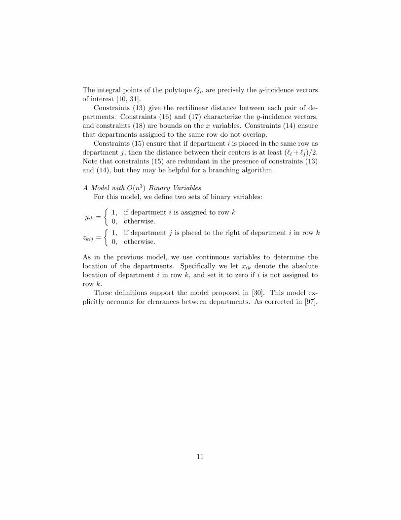
A Model with O(n3) Binary VariablesFor this model, we define two sets of binary variables:

yik =

{1, if department i is assigned to row k0, otherwise.

zkij =

{1, if department j is placed to the right of department i in row k0, otherwise.

As in the previous model, we use continuous variables to determine thelocation of the departments. Specifically we let xik denote the absolutelocation of department i in row k, and set it to zero if i is not assigned torow k.

These definitions support the model proposed in [30]. This model ex-plicitly accounts for clearances between departments. As corrected in [97],

11

the model is:

minn−1∑i=1

n∑j=i+1

cij

(v+ij + v−ij

)s.t.

∑k∈K

xik −∑k∈K

xjk + v+ij − v

−ij = 0, i ∈ I1, j ∈ I2 (19)

xik ≤Myik, i = 1, . . . , n, k ∈ K (20)∑k∈K

yik = 1, i = 1, . . . , n (21)

`iyik + `jyik2

+ aikzkji ≤ xik − xjk +M(1− zkji) (22)

i ∈ I1, j ∈ I2, k ∈ K`iyik + `jyik

2+ aikzkij ≤ xjk − xik +M(1− zkij), (23)

i ∈ I1, j ∈ I2, k ∈ K

zkij + zkji ≤1

2(yik + yjk), i ∈ I1, j ∈ I2, k ∈ K (24)

zkij + zkji + 1 ≥ yik + yjk, i ∈ I1, j ∈ I2, k ∈ K (25)

xik ≥ 0, i ∈ I, k ∈ Kv+ij , v

−ij ≥ 0, i ∈ I1, j ∈ I2

yik ∈ {0, 1}, i ∈ I, k ∈ Kzkij ∈ {0, 1}, i ∈ I, j ∈ I \ {i}, k ∈ K

(26)

where aij is the required clearance between departments i and j, I1 ={1, . . . , n − 1}, I2 = {i + 1, . . . , n}, K = {1, 2} is the set of rows, andthe constant M =

∑i∈I (`i + maxj∈I aij) is analogous to L in the previous

model but also includes the clearances.Constraints (19) compute the distances between departments. Con-

straints (20) set xik = 0 when department i is not assigned to row k.Constraints (21) ensure that a department is assigned to just one row. Con-straints (22) and (23) prevent departments from overlapping if they arelocated in the same row.

Constraints (24) and (25) ensure consistency between the variables yand z as follows: If yik = 1 and yjk = 1 then (24) and (25) together ensurethat exactly one of zkij and zkji is equal to one. Otherwise, i.e., if at leastone of yik and yjk is equal to zero, then (24) sets both zkij and zkji to zero.Constraints (25) force either zkij or zkji to be 1 if i and j are both in row k.

12

Note that the O(n2) model has significantly fewer variables than theO(n3) model, and that the meaning of the continuous variables xik differsbetween the two models. Finally, it is important to observe that while theO(n2) model is specific to the DRFLP, the O(n3) model can be applieddirectly to the MRFLP by increasing the cardinality of K.

2.2.2. SDO Model

An SDO-based approach for the MRFLP was developed in [47] and alsoapplied to the DRFLP. This approach is presented in Section 2.3.1.

2.3. The Multirow FLP

The MRFLP is a natural extension of row layout to three or more rows.An instance of the MRFLP has a given number of rows to which the depart-ments can be assigned, the departments all have the same height (equal tothe row height), the distances between adjacent rows are equal, and depart-ments can in general be assigned to any row.

The MRFLP has received very limited attention in the operations re-search literature to date. In terms of practical applications, it captures thebasic structure of contexts where the departments are to be arranged in well-defined rows because the separation between the rows is predetermined. Itis thus a problem that is discrete in one dimension and continuous in theother. Heuristic algorithms were proposed in [42], and a nonlinear opti-mization formulation was given in [36] and solved using a genetic algorithm(GA).

In terms of approaches using MILO and SDO, as noted in Section 2.2.1,the O(n3) MILO formulation of [97] for the DRFLP can be easily extendedto the MRFLP (this was not specifically done in that paper). More recently,an SDO-based approach was introduced in [47], and it is this approach thatwe present here. To the best of our knowledge, this is the only globaloptimization approach for the general row FLP with more than two rows.

2.3.1. SDO Model

The SDO model presented in [47] for the MRFLP is based on the SDOformulation for the SRFLP presented in Section 2.1.2. The idea is to firstassume that the assignment of departments to rows is fixed and that nospaces are allowed between departments in the same row. This restrictedversion of the MRFLP is called the k-Parallel Row Ordering Problem (k-PROP), see Section 2.3.2 and the references therein for more details.

Consider the k-PROP with n departments and m rows, and let the as-signment of departments to rows be specified by r : {1, . . . , n} → {1, . . . ,m}.

13

Define the binary variables Rij as in Section 2.1.2, and let dij represent thecenter-to-center distance between i and j measured parallel to the rows. Ifi and j are assigned to the same row, i.e., if r(i) = r(j), then

dij =1

2(`i + `j) +

∑k∈N, k<ir(k)=r(i)

`k1−RkiRkj

2+

∑k∈N, i<k<jr(k)=r(i)

`k1 +RikRkj

2

+∑

k∈N, k>jr(k)=r(i)

`k1−RikRjk

2,

(27)

while if r(i) 6= r(j)

dij = Rij

`j2 +

∑k∈N, k<jr(k)=r(j)

`k1 +Rkj

2+

∑k∈N, k>jr(k)=r(j)

`k1−Rjk

2

−

`i2 +∑

k∈N, k<ir(k)=r(i)

`k1 +Rki

2+

∑k∈N, k>ir(k)=r(i)

`k1−Rik

2

.

(28)

The above relations, plus the triangle inequalities relating the distancesbetween every triplet of departments i, j, k:

zij + zik ≥ zjk, zij + zik ≥ zjk, zik + zjk ≥ zij , 1 ≤ i < j < k ≤ n, (29)

are used in [47] to extend the SDO formulation for the SRFLP to an SDOformulation for the k-PROP. For the sake of brevity here, we refer the readerto [47] for the technical details.

Once an SDO formulation of the k-PROP is obtained, the possibility ofspaces is handled using the following results:

Theorem 1 ([47]). If all the department lengths `i are integer, then thereis always an optimal solution to the MRFLP on the half-integer grid.

Corollary 1 ([47]). If all the department lengths `i are integer, then for eachinstance of the MRFLP, we obtain an equivalent instance of the k-PROP byadding spacing departments of length 0.5 such that the length of each rowbecomes equal to M :=

∑ni=1 `i.

14

The strategy is thus to add spacing departments of length 0.5 and withall involved connectivities equal to zero, and then apply the SDO approachfor k-PROP. Because the number of spacing departments needed will nor-mally be too large for practical computation, several results are proved inHungerlander and Anjos [47] to reduce the number of spacing departmentsneeded.

Finally, to remove the restriction that the assignment of departments torows is fixed, Hungerlander and Anjos [47] obtain global optimal solutions(respectively bounds) by using this approach for all possible assignments(respectively for a subset of them).

2.3.2. Special Cases of the MRFLP

The difficulty in solving the general MRFLP has motivated the studyof a number of special cases with simplifying assumptions and/or specificstructure that allow for more effective modeling and solution approaches.

The Equidistant MRFLPA first such special case is the equidistant version of the MRFLP, denoted

MREFLP, in which all departments have the same length. This structuremakes it possible to prove many interesting results. The single-row case isknown in the literature as the linear arrangement problem, see e.g. [63],[11], [12], [80], [6], and is well known to be NP-hard even if all the pairwisecosts are binary [35].

The double-row case was considered in [7] where a MILO formulationbased on the quadratic assignment problem is given.

For the general MREFLP, it is shown in [16] that the problem has anoptimal solution on the integer grid (although the lengths of the spaces are ingeneral continuous quantities). This implies that only spaces of unit lengthneed to be used when modeling the MREFLP, and hence that the problemcan be formulated as a purely discrete optimization problem, as is the casefor the SRFLP in Section 2.1. Moreover, exact results were proved in [16]for the minimum number of spaces that must be added so as to preserveat least one optimal solution. These results lead to both MILO and SDOmodels for the MREFLP.

The Space-Free MRFLPAnother important special case of the MRFLP is the Space-Free MRFLP

(SF-MRFLP) in which no spaces are allowed within the rows, all rows havea common left origin, and the leftmost department in each row is flush withthe left end of the row. When there is only one row, the SF-MRFLP is

15

equivalent to the SRFLP. Where there are two rows, the SF-MRFLP is alsocalled the Space-Free DRFLP or the Corridor Allocation Problem, for whicha MILO formulation was proposed in [8], and an SDO approach in [46].

A special case of the SF-MRFLP that has attracted attention is the k-PROP introduced in Section 2.3.1. Because the assignment of departmentsto rows is given, and no spaces are allowed within the rows, the k-PROPreduces to finding the optimal permutation of the departments within eachrow. An SDO approach for k-PROP was mentioned in Section 2.3.1, andanother was given in [45]. When the number of rows equals two, this problemis simply called PROP, and a MILO formulation for it was given in [9].

2.4. Computational Performance of the Models

Row FLPs remain highly challenging problems. We summarize here thestate-of-the-art in terms of the computational performance of the approachespreserved above.

For both the SRFLP and the single-row MREFLP, the largest instancessolved to optimality had 42 departments, see [48] and [44] respectively.

For the DRFLP, the O(n2) model was used in [10] to obtain solutionsof instances with up to 12 departments within one hour. The O(n3) modelwas also tested in [10] but was unable to solve instances with more than 10departments within three hours. The corrected model of [97] was used in[76] for asymmetric flows. The constraints are (20)–(26), and the objectivefunction is ∑

i∈I1

∑j∈I2

(cij + cji)(v+ij + v−ij

).

The conclusion of the computational tests is that with a time limit of 10minutes, most of the heuristic algorithms perform better than CPLEX oninstances with more than 20 departments.

Finally for the MRFLP, tight global bounds were computed in [47] forinstances with up to 12 departments. The authors adapted an approachoriginally proposed in [34] for the max-cut problem and several orderingproblems. The SDO-based approach was applied to instances with up to 5rows and up to 8 departments. The results show that the SDO approach ismost effective for 4 or 5 rows. There may be an intuitive explanation forthis: as an extreme example, note that it is easier to partition 5 departmentsinto 5 rows than into 2 rows. This is in part because the model does not takeinto account the distance between rows, so assigning department 1 to row1 is exactly the same as assigning it to row 4. Accounting for the distancesbetween rows may change the nature of the results, but has not yet beendone to the best of our knowledge.

16

3. Unequal-Areas FLP

The Unequal-Areas FLP (UA-FLP) is concerned with finding the opti-mal arrangement of a given number of nonoverlapping indivisible depart-ments with varying areas so as to minimize the total expected cost of flowsinside the facility. Unlike in the row FLPs, the dimensions of each depart-ment are optimized (subject to the area requirement).

The UA-FLP, sometimes called the single-floor FLP, has received muchattention in the literature. It was first stated in [23], and one of the firstMILO formulations was proposed in [74] using binary variables to preventoverlap.

We begin with an exact formulation of the UA-FLP in Section 3.1. Thisallows us to establish notation, and more importantly to explicitly showwhere the main difficulties are for solving UA-FLP. Exact MILO modelsare covered in Section 2.2.1. This includes sequence-pair formulations inSection 3.2.1, one of which solved instances with up to 11 departments toglobal optimality, the largest such results to date [72].

Most of the approaches reviewed here are two-stage frameworks, wherethe first stage determines the relative location of the departments, and thesecond stage obtains a final layout via a mathematical optimization model.Two-stage approaches are mathematical optimization-based heuristics thatare not guaranteed to find the global optimal layout but they seem to bethe most promising for handling large-scale instances of UA-FLP. The maindifferences between the approaches are in the first-stage algorithms. Wepresent in Section 3.3 approaches that are entirely based on nonlinear op-timization models, one of which was recently shown to be able to computelayouts for instances with up to 100 departments in less than 15 min of com-putation time [22]. Other two-stage approaches are summarized in Section3.4.

A MILO formulation for the important special case of flexible bay UA-FLP is discussed in Section 3.5

A number of heuristics for the UA-FLP make use of a slicing-tree struc-ture. This is a binary tree that represents the floor plan after applying arecursive partitioning process. Each node of the tree contains either a de-partment or a cut operator, thus each slicing tree corresponds to a particularlayout. This strategy was first used in [79] in the context of VLSI design andlater extended to the UA-FLP in [93]. It was also used in [85, 33, 84, 55, 29].

17

3.1. An Exact Formulation of the UA-FLP

We begin by presenting an exact formulation that uses only continuousvariables. The reasons for doing so are two-fold: we establish some notationthat will be common for the remainder of this section, and we explicit pointout where the difficulties lie in solving UA-FLP, thus motivating the solutionapproaches subsequently presented.

We assume that we are given the height and width of the facility ashF and wF respectively, and that for each department i we have lower andupper bounds wmin

i and wmaxi on its width, and hmin

i and hmaxi on its height.

We also assume that βi, an upper bound on the aspect ratio of departmenti, is given for each department i. It is necessary that βi ≥ 1, and the closerβi is to unity, the closer the shape of department i will be to a square.

With this notation, the UA-FLP can be formulated as follows (see [94]):

minxi,yi,hi,wi

∑1≤i<j≤n

cij(|xi − xj |+ |yi − yj |) (30)

s.t. wmini ≤ wi ≤ wmax

i , for i = 1, . . . , n (31)

hmini ≤ hi ≤ hmax

i , for i = 1, . . . , n (32)

wihi = Ai, for i = 1, . . . , n (33)

max

{wihi,hiwi

}≤ βi, for i = 1, . . . , n (34)

xi +1

2wi ≤

1

2wF and

1

2wi − xi ≤

1

2wF , for i = 1, . . . , n (35)

yi +1

2hi ≤

1

2hF and

1

2hi − yi ≤

1

2hF , for i = 1, . . . , n (36)

|xi − xj | ≥1

2(wi + wj) or |yi − yj | ≥

1

2(hi + hj),

for all 1 ≤ i < j ≤ n.(37)

The first four sets of constraints enforce the shape requirements. Constraints(31) and (32) enforce the bounds on the width and height of each depart-ment. Constraints (33) enforce the area requirement for each department.Note that these constraints can be relaxed to wihi ≥ Ai. This relaxed formhas the advantage of being convex, and in fact it can be formulated as aconic constraint (see Section 3.2). Because the optimization will push thisrelaxed form towards equality, in general wihi will equal Ai at optimality.Moreover Theorem 3.1 in [92] states that if

∑ni=1Ai = hFwF then the con-

straints 33 must hold at every feasible solution. Constraints (34) enforcethe maximum aspect ratio; it is straightforward to write them as two linearinequality constraints.

18

The last two sets of constraints enforce the location requirements. Con-straints (35)–(36) ensure that the departments are inside the facility. Fi-nally, constraints (37) prevent overlapping; these constraints are disjunctiveand nonconvex, and are the hardest ones to handle. If the relative posi-tion of each pair of departments is known, then the constraints (37) canbe written as linear inequalities, and the formulation becomes a (convex)conic optimization problem that is straightforward to solve. This observa-tion motivates the two-stage philosophy in several of the approaches in theliterature; we present the most prominent in Sections 3.3 and 3.4.

Note that this formulation locates the center of the facility at the origin,while some of the models below locate the origin at the bottom left-handcorner of the facility. This difference is otherwise of no consequence.

3.2. MILO Models

We begin with the MILO model introduced by [73] and enhanced in [88].Define the binary variables

zhij =

{1 if i must precede j horizontally,0 otherwise,

zvij =

{1 if i must precede j vertically,0 otherwise.

19

The MILO formulation is as follows:

min∑

1≤i<j≤ncij(uij + vij) (38)

s.t.uij ≥ xi − xj and uij ≥ xj − xi, 1 ≤ i < j ≤ nvij ≥ yi − yj and vij ≥ yj − yi, 1 ≤ i < j ≤ n

(39)

1

2wi ≤ xi ≤ wF −

1

2wi, i = 1, . . . , n

1

2hi ≤ yi ≤ hF −

1

2hi, i = 1, . . . , n

(40)

wmini ≤ wi ≤ wmax

i , i = 1, . . . , n

hmini ≤ hi ≤ hmax

i , i = 1, . . . , n(41)

aiwi + 4

(wmini +

λ

∆− 1(wmax

i − wmini )

)2

hi ≥

2ai

(wmini +

λ

∆− 1(wmax

i − wmini )

), λ = 0, 1, . . . ,∆− 1

(42)

zhij + zhji + zvij + zvji = 1, 1 ≤ i < j ≤ n (43)

xi +1

2wi ≤ xj −

1

2wj + wF (1− zhij), i 6= j

yi +1

2hi ≤ yj −

1

2hj + hF (1− zvij), i 6= j

(44)

zhij , zvij ∈ {0, 1}, i, j ∈ N. (45)

Constraints (39) provide a linearization of the objective function (30) above.Constraints (40) ensure that each department is within the facility; theydiffer from (35)–(36) because this formulation places the origin at the bottomleft-hand corner of the facility. Constraints (41) are lower and upper boundsfor the widths and heights of the departments.

Constraints (42) are the polyhedral outer approximation on ∆ points of(33). This approximation was introduced in [88] and also used in [72] and[62] (see Section 3.2.1 below). This approximation is effective in practicebut less efficient that using the aforementioned convex conic relaxation thatis supported by most current MILO solvers. This is because wihi ≥ Ai isequivalent to a second-order cone constraint:[

hi√Ai√

Ai wi

]� 0⇔ wi + hi ≥

∥∥∥∥( wi − hi2√Ai

)∥∥∥∥2

. (46)

Finally, constraints (43)–(45) use the relative-location variables zhij and

20

zvij to prevent overlapping: depending on which of the variables zhij , zvij , z

hji, z

vji

is set to 1, i is to the left of, to the right of, below, or above j.An alternative MILO representation of the relative positions of depart-

ments is given in the next section.

3.2.1. Sequence-Pair Formulations

Sequence-pair approaches determine the relative positions of the depart-ments using the so-called sequence-pair representation, and combine thisrepresentation with a MILO model similar to the one above to obtain theoptimal layout. The sequence-pair representation was first used for VLSIdesign in [75], and for the FLP in [72] and [62].

A sequence-pair is a pair of sequences of departments, denoted Γ+ andΓ−, that together encode the relative location of the departments. Thefollowing theorem indicates how to translate a sequence-pair into a layout.

Theorem 2 ([72]). Given a sequence-pair (Γ+,Γ−) and two departments iand j in (Γ+,Γ−), i and j satisfy the following horizontal/vertical relation-ship in the FLP:

- if j succeeds i in both Γ+ and Γ−, then j is to the right of i;

- if j precedes i in both Γ+ and Γ−, then j is to the left of i;

- if j precedes i in Γ+ and succeeds i in Γ−, then j is above i;

- if j succeeds i in Γ+ and precedes i in Γ−, then j is below i.

The sequence-pair structure can be incorporated in a MILO model asfollows. Given a sequence-pair (Γ+,Γ−) and departments i and j, define thebinary variables:

z+ij =

{1 if i precedes j in Γ+,0 otherwise,

z−ij =

{1 if i precedes j in Γ−,0 otherwise.

These definitions lead to Theorem 3:

Theorem 3 ([72]). For any two departments i and j, the following hold:

- if z+ij = 1 and z−ij = 1, then i precedes j horizontally;

- if z+ij = 0 and z−ij = 0, then j precedes i horizontally;

- if z+ij = 0 and z−ij = 1, then i precedes j vertically;

- if z+ij = 1 and z−ij = 0, then j precedes i vertically.

21

A different MILO model (see [72]) for the FLP can now be formulated:

min∑

1≤i<j≤ncij(uij + vij)

s.t. (39)–(42)

z+ij + z+

ji = 1, 1 ≤ i < j ≤ nz−ij + z−ji = 1, 1 ≤ i < j ≤ n

(47)

z+ik + z+

kj − z+ij ≤ 1, 1 ≤ i < j ≤ n

z−ik + z−kj − z−ij ≤ 1, 1 ≤ i < j ≤ n

(48)

xi +1

2wi ≤ xj −

1

2wj + wF (2− z+

ij − z−ij), i, j ∈ N, i 6= j

yi +1

2hi ≤ yj −

1

2hj + hF (1 + z+

ij − z−ij), i, j ∈ N, i 6= j

(49)

z+ij , z

−ij ∈ {0, 1}, i, j ∈ N. (50)

Constraints (47) ensure that every department appears exactly once in eachsequence, and constraints (48) are transitivity constraints for the two se-quences. Together these constraints ensure that the binary variables repre-sent valid sequences. Constraints (49) express nonoverlapping in terms ofthe sequence-pair variables.

Using the MILO model above with additional valid inequalities, includ-ing p − k symmetry-breaking constraints (see Section 5), instances of UA-FLP with up to 11 departments were solved to global optimality in [72]. Thecomputational time reached almost 17 hours for the 11-department instance.

Castillo and Westerlund [27] proposed a MILO model that satisfies thearea requirements within a given accuracy ε using cutting planes. We omitthe details for this because the area constraints can be handled more effec-tively using conic optimization, as mentioned above. We point out howeverthat Castillo and Westerlund [27] used the following alternative formulationof nonoverlap that is essentially the sequence-pair representation:

1

2(wi + wj)− (xi − xj) ≤ wF (Xij + Yij), 1 ≤ i < j ≤ n (51)

1

2(wi + wj)− (xj − xi) ≤ wF (1 +Xij − Yij), 1 ≤ i < j ≤ n (52)

1

2(hi + hj)− (yi − yj) ≤ hF (1−Xij + Yij), 1 ≤ i < j ≤ n (53)

1

2(hi + hj)− (yj − yi) ≤ hF (2−Xij − Yij), 1 ≤ i < j ≤ n (54)

Xij , Yij ∈ {0, 1}, 1 ≤ i ≤ n, (55)

22

where the variables Xij and Yij are a binary codification of the relative po-sition of departments. A GA was implemented in [62] where each sequence-pair is a chromosome; the sequence-pair gives the relative position of thedepartments (first stage), and then a LO model is solved to find the bestlayout (second stage). They achieved the best results up to then for in-stances with up to 35 departments; the computational time was 26 hoursfor the 35-department instance.

A branch-and-bound algorithm that uses the sequence-pair representa-tion was presented in [96]. A minimum-cost network flow problem is solvedto obtain a feasible layout from the sequence-pair representation of the rel-ative position layout. However, this is only valid for a restricted version ofthe UA-FLP in which the department widths and heights are fixed, and thefacility has no limitations. Such an UA-FLP with just the nonoverlappingconstraints can be transformed into a network flow problem. The advantageis that network flow algorithms can be several orders of magnitude fasterthan general LO algorithms.

It was observed in [72] and [62] that the MILO model with constraints(43) and (45) has 2n(n−1) possible combinations of the binary variables, whilethe sequence-pair-based MILO formulation has (n!)2 sequences generatingthe same set of relative-position combinations. The authors claim that thisdifference is key to the effectiveness of the sequence-pair approach. The dif-ference is indeed significant: Using Stirling’s approximation, we have that(n!)2 = θ(e2(n ln(n)−n)) while 2n(n−1) = e0.693(n2−n). However, a comparisonof the two formulations shows that another important difference is the pres-ence of the transitivity constraints (48) in the sequence-pair model. It isnot entirely clear to what extent each of these differences contributes to theefficiency of the sequence-pair approach. It would be interesting to carryout a computational study to clarify this question.

3.3. Two-Stage Approaches Using Nonlinear Optimization

A two-stage approach based on the attractor-repeller (AR) techniquefor VLSI floorplanning was introduced in [19]. The first stage uses the ARtechnique to establish the relative positions of the departments, and thesecond stage finds a feasible layout satisfying the relative positions specifiedby the solution to the first stage. The objective of this approach is notto achieve global optimality but rather to efficiently compute competitivesolutions to large-scale instances of UA-FLP.

The AR model approximates each department by a circle with radius riproportional to the square root of Ai. The model places the circles insidethe facility while allowing some overlapping. The amount of overlapping is

23

controlled via a so-called target distance: given α > 0, the target distancetij for circles i and j is set as tij = α(ri + rj)

2. The AR model is:

minx,y

∑1≤i<j≤n

cijDij + f

(Dij

tij

)s.t. xi + ri ≤

1

2wF , i = 1, . . . , n

xi − ri ≥ −1

2wF , i = 1, . . . , n

yi + ri ≤1

2hF , i = 1, . . . , n

yi − ri ≥1

2hF , i = 1, . . . , n,

where (xi, yi) is the center of circle i, Dij = (xi − xj)2 + (yi − yj)

2 andf(z) = 1

z − 1 is a penalty function. The constraints keep the circles insidethe facility whose center is at the origin. The objective function is a trade-off

between the attractor term cijDij and the repeller term f(Dij

tij

).

While the constraints are linear, the objective function is nonlinear and

nonconvex. It was convexified in [19] by replacing the term cijDij +f(Dij

tij

)with the following piecewise function:

fij(xi, xj , yi, yj) =

cijz +tijz − 1, z ≥

√tijcij

2√cijtij − 1, 0 ≤ z <

√tijcij

(56)

where z = (xi − xj)2 + (yi − yj)2, and it is assumed that cij > 0. Note thatthe second branch of fij is constant, and that by construction, fij attainsits minimum whenever the positions of i and j satisfy Dij ≤

√tij/cij . This

includes the case where Dij = 0, i.e., the two circles completely overlap. Ofcourse, such a placement is undesirable. The ideal arrangement of the circleshas Dij ≈

√tij/cij , i.e., close to the boundary of the flat portion of fij . At

these points, the minimum of fij is attained at the same time as the overlapis minimized. This motivates the introduction in [20] of a generalized targetdistance:

Tij =

√tij

cij + ε, 1 ≤ i, j ≤ n, (57)

where ε > 0 is chosen sufficiently small so that Tij ≈√tij/cij . This modifi-

cation also removes the need for the assumption that cij > 0.

24

In practice, attaining a solution with Dij ≈ Tij is not easy. The approachin [20] sacrifices convexity and proposes a modified AR model with theobjective:

min∑

1≤i<j≤nfij(xi, xj , yi, yj)−K log

{Dij

Tij

}, (58)

where

fij(xi, xj , yi, yj) =

{cijz +

tijz − 1, z ≥ Tij

2√cijtij − 1, 0 ≤ z < Tij ,

and the logarithmic term steers the optimization away from solutions withDij ≈ 0. Indeed the minima of this (nonconvex) function satisfy Dij ≈ Tij .This can be viewed as a compromise in the sense that convexity is lost, butcomputational efficiency is gained because a suitable choice of starting pointand nonlinear optimization solver makes it possible to compute a solutionclose to these known minima.

In the second stage, the nonoverlapping constraints (37) are formulatedas complementarity constraints. For each pair i, j, we introduce new vari-ables Xij and Yij satisfying

Xij ≥1

2(wi + wj)− |xi − xj |, Xij ≥ 0,

Yij ≥1

2(hi + hj)− |yi − yj |, Yij ≥ 0,

XijYij = 0

This last constraint enforces nonoverlap by requiring that at least one ofXij and Yij equal zero. Using the coordinates of the centers of the circlesin the optimal solution of the modified AR model to initialize the nonlinearoptimization solver, this approach improved on the then-best-known solu-tions for large instances, in particular for the Armour-Buffa 20-departmentinstance.

There are some challenges with this approach so far. First a nonconvexmodel with the repeller function 1

z − 1 was proposed in [19]; this model wasthen modified in [20] to achieve convexity, but then the addition of a newpenalty term resulted again in a loss of convexity, though in a more con-trolled manner. Moreover, the optimization problem with complementarityconstraints is difficult to solve for large-scale instances.

This motivated the significant improvements to this approach carriedout in [50]. For the first stage, fij(xi, xj , yi, yj) is replaced by a more com-plicated expression that also integrates information about the aspect ratio

25

constraints. We refer the reader to [50] for details on the first stage, andinstead present below the recent further improvements in [22].

The more significant contributions in [50] are their improved secondstage, and the linking of the two stages. They introduce the following convexsecond-stage model that can be solved efficiently:

min(xi,yi),wi,hi

∑1≤i<j≤n

(uij + vij) (59)

s.t. uij ≥ xi − xj , for 1 ≤ i < j ≤ n (60)

uij ≥ xj − xi, for 1 ≤ i < j ≤ n (61)

vij ≥ yi − yj , for 1 ≤ i < j ≤ n (62)

vij ≥ yj − yi, for 1 ≤ i < j ≤ n (63)

wmini ≤ wi ≤ wmax

i , for 1 ≤ i < j ≤ n (64)

hmini ≤ hi ≤ hmax

i , for 1 ≤ i < j ≤ n (65)

wihi ≥ Ai, for 1 ≤ i < j ≤ n (66)

βiwi − hi ≥ 0, for 1 ≤ i < j ≤ n (67)

βihi − wi ≥ 0, for 1 ≤ i < j ≤ n, (68)

plus appropriately chosen linear inequality constraints to ensure nonoverlap.These nonoverlap constraints are obtained as follows. Consider the coor-

dinates of the centers of the circles in the optimal solution to the first stageas a set of points on the plane, and compute their Delaunay triangulation.One of the properties of this triangulation is that it maximizes the minimumangle over all the angles of the triangles; in practice this means that thintriangles are less likely. The edges of the Delaunay triangulation are takento represent the relative positions of the departments, and these positionsare then enforced by the appropriate linear constraints. For example, if thecenters of i and j are connected in the triangulation and j is to the rightof i, then the constraint xj − xi ≥ 1

2(wi + wj) is added to the model. Theresult is a second stage model that is a conic optimization problem and canbe solved efficiently.

The overall approach in [50] provided further improved layouts for theclassical Armour-Buffa instance, and computed high-quality layouts for sev-eral 30-department instances in 5 minutes or less of computation time.

Most recently, [22] further developed the AR concept. As the secondstage of [50] is highly effective, the novelty in [22] is the formulation of thefirst stage. Specifically they propose a more precise formulation that modelsthe departments as rectangles instead of approximating them by circles. The

26

aspect ratio constraints can therefore be exactly enforced at the first stage,instead of being approximated as in [50]. They still forego convexity anduse the simple objective function

cijD2ij +K

θ2ij

D2ij

− 1,

where θ2ij = 1

4

((wi + wj)

2 + (hi + hj)2). Note that Dij/θij ≈ 1 indicates

that some of the borders of the rectangles are close, regardless of whetherthe rectangles are overlapping (by a small amount) or not.

The resulting first-stage model is:

minxi,yi,hi,wi

∑1≤i<j≤n

(cijD

2ij +K

θ2ij

D2ij

− 1

)

s.t. xi +1

2wi ≤

1

2wF and

1

2wi − xi ≤

1

2wF , for i = 1, . . . , n,

yi +1

2hi ≤

1

2hF and

1

2hi − yi ≤

1

2hF , for i = 1, . . . , n,

wihi ≥ Ai, for i = 1, . . . , n,

βwi − hi ≥ 0, for i = 1, . . . , n,

βhi − wi ≥ 0, for i = 1, . . . , n,

wmini ≤ wi ≤ wmax

i , for i = 1, . . . , n,

hmini ≤ hi ≤ hmax

i , for i = 1, . . . , n.

where K = α∑

1≤i<j≤n cij , and 0 < α ≤ 1. By solving for different choicesof α (and hence of K), the authors of [22] improved on the best solutions byearlier techniques. Furthermore, they computed layouts for instances withup to 100 departments in less than 15 min of computation time. This is theonly approach entirely based on mathematical optimization models that hasbeen able to reach such large-scale instances of UA-FLP.

3.4. Other Two-Stage Approaches

A heuristic based on a graph-pair representation and a simulated an-nealing technique was proposed in [25]. One of the graphs represents thehorizontal separation of the departments, and the other represents the ver-tical separation. Their results are generally good, but the authors makechanges in the areas of the facilities or departments. These modificationsare reasonable from a practical point of view, but they make it difficult tocompare with other techniques.

27

A LO-based GA approach, which differs from [62] in the chromosomecoding, was introduced in [58]. The idea is that the GA searches for the rel-ative locations of the departments, and the LO model determines their exactlocations and shapes. In particular, a new location/shape representation isproposed to encode the relative locations. Specifically, the relative locationof department i is represented as (xi, yi, αi), where αi = hi/wi. For each(xi, yi, αi), define two straight lines, one passing through (xi, yi) and the up-per right corner (xi+wi/2, yi+hi/2), and the other passing through (xi, yi)and the upper left corner (xi−wi/2, yi +hi/2). These lines split the facilityinto four regions with reference to department i, so every other departmentis above or below or left or right of i. Like the sequence-pair representation,the location/shape representation always generates a consistent assignmentof the binary decision variables. Note that while the MILO-model does notcontain the transitivity constraints for the integer variables, this encoding(based on continuous variables) encapsulates transitivity. The results in [58]show that this approach outperforms previous techniques: the cost functionis reduced and the computational time is lower.

A similarly structured approach was proposed in [37] using a random-key GA in the first stage and a LO model in the second stage. The authorsreport results on several instances of UA-FLP from the literature, and findslightly better solutions in a considerably shorter computational time, incomparison with the other GA approaches. They also applied their approachto larger instances with up to 125 departments, but without restrictions onthe dimensions of the facility. The computational time is reduced becausethey do not solve all the LO problems originating from the relative-positionsolutions: they only solve the problems that provably yield a feasible solutionwith a cost not exceeding 40% of that of the previous best solution.

3.5. Flexible Bay Structure

A flexible bay structure is a continuous layout where the departments arelocated in parallel bays with flexible widths. This special case of the UA-FLParises in manufacturing facilities [69]. The bay structure is similar to therow structure in row FLPs, but a fundamental difference is that the width ofeach bay depends on the total area of the departments in that bay, whereasin row FLPs, the heights of the rows and of the departments are equal andfixed. The bays have straight aisles on both sides, and departments are notallowed to span multiple bays. This structure restricts the set of feasiblesolutions, but it has advantages in practice: the bay boundaries form thebasis of an aisle structure that facilitates the transfer of the layout solutionto an actual facility design.

28

A MILO formulation for this problem was proposed in [56]. The continu-ous variables xi, yi represent the location of department i, and hik representthe height of department i in bay k. The binary variables are defined asfollows:

zik =

{1, if department i is assigned to bay k0, otherwise;

rij =

{1, if department i is above department j in the same bay0, otherwise;

δk =

{1, if bay k is occupied0, otherwise.

29

The MILO model is:

min∑

1≤i<j≤ncij(uij + vij)

s.t. uij ≥ xi − xj and uij ≥ xj − xi, 1 ≤ i < j ≤ nvij ≥ yi − yj and vij ≥ yj − yi, 1 ≤ i < j ≤ n∑k∈K

zik = 1, i ∈ N (69)

wk =1

hF

∑i∈N

zikAi, k ∈ K (70)

wmini zik ≤ wk ≤ wmax

i + wF (1− zik), k ∈ K, i ∈ N (71)

xi ≥∑j≤k

wj − 0.5wk − (wF − wmini )(1− zik), k ∈ K, i ∈ N

xi ≤∑j≤k

wj − 0.5wk + (wF − wmini )(1− zik), k ∈ K, i ∈ N

(72)

hikAi−hjkaj−max

{`maxi

Ai,`minj

aj

}(2− zik − zjk) ≤ 0, i < j

hikAi−hjkaj

+ max

{`maxi

Ai,`minj

aj

}(2− zik − zjk) ≤ 0, i < j

(73)

∑i∈N

hik = hF δk, k ∈ K (74)

hmini zik ≤ hik ≤ hmax

i zik, i ∈ N, k ∈ K (75)∑i∈N

hik = hi, i ∈ N (76)

yi − 0.5hi ≥ yj + 0.5hj − wH(1− rij), i 6= j (77)

rij + rji = 1, 1 ≤ i < j ≤ n (78)

rij + rji ≥ zik + zjk − 1, 1 ≤ i < j ≤ n, k ∈ K (79)

0.5hi ≤ yi ≤ wH − 0.5hi, i ∈ N. (80)

where K is the set of bays, and N is the set of departments.Constraints (69) ensure that each department is assigned to a single

bay. Constraints (70) calculate the width of each bay as the total area ofthe departments assigned to that bay divided by the facility height. Notethat under the assumption that

∑i∈N

Ai ≤ wFhF , we have∑k∈K

wk ≤ wF .

Constraints (71) impose bounds on the bay widths, based on the width

30

bounds of the departments assigned to each bay. Constraints (72) determinethe horizontal locations of the department centroids. In this model, the x-coordinate is located at the middle of the bays. Therefore, if department iis assigned to bay k, xi is calculated as xi =

∑kj=1wj − 0.5wk. This agrees

with constraints (72) with zik = 1. If i and j are in the same bay k, thenconstraints (73) ensure that the widths of the two departments are the sameand equal to the bay width. Constraints (74) set the total heights of thedepartments in a bay equal to hF if the bay is used, and zero if the bay isempty. Constraints (75) are bounds on the department heights. They alsoenforce hik = 0 when department i is not located in bay k. Constraints(76) define the heights of the departments. Constraints (78)–(79) ensurethat department i is either above or below department j. Constraints (77)prevent departments in the same bay from overlapping. Constraints (80)ensure that the departments are inside the facility.

By adding symmetry-breaking constraints (see Section 5) and valid in-equalities (see Section 6), instances with up to 14 departments were solvedto optimality in [56]. The 14-department instance needed around 120 hoursof computational time.

4. Multifloor FLP

The multifloor FLP (MF-FLP) involves finding the optimal arrangementof departments in a facility with multiple floors. Practical applications in-clude production facilities, hotels, office buildings, and hospitals. This prob-lem has added complexity in comparison to the UA-FLP because we mustalso consider the interactions between departments on different floors. Fur-thermore, elevators and/or stairwells are required to transfer people and/ormaterial between the floors, and these need to be placed at coherent loca-tions in every floor that they reach.

Globally optimal algorithms for MF-FLP work in general only for smallinstances [38]. The problem was first investigated in [51] and later in [70],but most of the subsequent models in the literature are designed for specifictypes of MF-FLP, as the literature survey in Section 4.1 shows. Indeedthere is no commonly agreed definition of the MF-FLP because differentauthors make their own assumptions about the structure of the problem.This lack of a common definition makes it hard to compare the approaches.We therefore propose in Section 4.2 a general formulation for the MF-FLPthat we hope will gain acceptance as a standard formulation, and will leadto increased research activity on this problem.

31

4.1. Survey of the Literature

Some approaches first distribute the departments over the floors, min-imizing the vertical interaction costs. This is essentially the first stage ofa two-stage approach, where the second stage then optimizes the layout ofeach floor independently; see [70] and [24]. Specifically the following MILOformulation is used in [69] to assign departments to floors:

min∑

1≤i<j≤ncijd

vij (81)

s.t.

p∑k=1

zik = 1, 1 ≤ i ≤ n (82)

dvij ≥ δp∑

k=1

k(zik − zjk), 1 ≤ i < j ≤ n (83)

dvij ≥ δp∑

k=1

k(zjk − zik), 1 ≤ i < j ≤ n (84)

n∑i=1

Aizik ≤ wF hF , 1 ≤ k ≤ p (85)

zik ∈ {0, 1}, 1 ≤ i ≤ n, 1 ≤ k ≤ p, (86)

where p is the number of floors. The variable zik equals 1 if departmenti is assigned to floor k, and equals 0 otherwise. Constraints (82) assigneach department to exactly one floor. Constraints (83)-(84) compute thevertical distance dvij between each pair i, j of departments, where δ is thefloor height. Note that ∣∣∣∣∣

p∑k=1

k(zik − zjk)

∣∣∣∣∣is precisely equal to the number of floors separating i and j. Constraints(85) ensure that the departments assigned to each floor fit into that floor.

Each floor then becomes an instance of UA-FLP with some additionalconstraints to ensure coherence in the location of the elevators. Computingthe vertical costs still remains a challenge and was addressed in [24].

Another possible simplification is to restrict all the departments to havethe same shape and to require that they be assigned to specific locationsin the building. This reduces the problem to a quadratic assignment prob-lem. Such a formulation was used in [38], and was solved using the RLTlinearization technique [1, 86] within a branch-and-bound algorithm.

32

A mathematical formulation of MF-FLP for process plant layout waspresented in [82]. Its objective function considers the construction and landcosts to decide the number of floors and the floor area. Another model for aprocessing plant was proposed in [32]; it incorporates many structural andoperational issues, but becomes unwieldy.

A GA is also used in [61] to find a layout with inner walls and pas-sages. The connections between the departments, passages, and elevatorsare represented as an adjacency graph, and the distances are calculated us-ing Dijkstra’s algorithm. This representation allows the measurement ofthe distances of paths that use corridors and elevators. The bi-objectivemodel minimizes the total cost of transporting the materials and maximizesthe adjacency achieved. It is applied to a multideck ship layout with innerwalls.

Another bi-objective model is proposed in [40] for a MF-FLP formulationthat minimizes not only the material handling costs (as usual) but also thefacility construction costs. This model is similar to the one we present inSection 4.2, but a major difference is that the length and width of the facility,the number of elevators, and the number of floors are decision variables.

For completeness, we also mention the robust model in [49] in whichsome of the usual parameters are considered to be uncertain, and the modelin [81] that takes into account safety distances in the event of an explosion.

4.2. A MF-FLP Formulation

We assume that the following parameters are given: the number of de-partments and their areas, the number of floors, the dimensions and heightof the floors, the interconnection costs, and the number and size of the el-evators. We consider the elevators to be a general system (incorporatingelevators, stairs, pipes, etc.) for vertical movement. We want to determinethe locations of the elevators and the locations and dimensions of the de-partments. The horizontal distance is the rectilinear distance (which is areliable measure, as in the single-floor case), and the vertical distance willbe measured using the elevators. This makes the formulation complex. Thenumber of floors and elevators is assumed to be fixed; if necessary, we couldrun the model for several different options. The floor dimensions are fixed,but they could easily be treated as decision variables.

Let δ denote the ceiling height, p the number of floors, and e the numberof elevators. Let also M = wF + hF + δp. Define the following variables:zik = 1 if department i is assigned to floor k, 0 otherwise;

Zij = 1 if departments i and j are allocated to the same floor, 0 otherwise;

Xij , Yij : nonoverlapping binary variables;

33

(xi, yi): coordinates of the centroid of department i;

dvij : vertical distance between i and j;

dhij : horizontal distance between i and j located on the same floor;

deij : horizontal distance between i and j located on different floors, wherethe path includes an elevator.

Note that the indices n+ 1, . . . , n+ e correspond to the elevators.The formulation is as follows:

min∑

1≤i<j≤ncij(d

eij + dvij)

s.t.

p∑k=1

zik = 1, 1 ≤ i ≤ n (87)

dvij = δ

∣∣∣∣∣p∑

k=1

k(zik − zjk)

∣∣∣∣∣ , 1 ≤ i < j ≤ n

dhij = |xi − xj |+ |yi − yj |, 1 ≤ i < j ≤ ndeij ≥ dhij , 1 ≤ i < j ≤ ndeij ≥ |xi − x`|+ |yi − y`|+ |xj − x`|+ |yj − y`| −MZij ,

1 ≤ i < j ≤ n, n+ 1 ≤ ` ≤ n+ e

(88)

Zij ≥ zik + zjk − 1, 1 ≤ i < j ≤ n, k = 1, . . . , p

Zij ≤ 1− zik + zjk, 1 ≤ i < j ≤ n, k = 1, . . . , p

Zij ≤ 1 + zik − zjk, 1 ≤ i < j ≤ n, k = 1, . . . , p

(89)

xi +1

2wi ≤

1

2wF , xi −

1

2wi ≥ −

1

2wF , 1 ≤ i ≤ n+ e

yi +1

2hi ≤

1

2hF , yi −

1

2hi ≥ −

1

2hF , 1 ≤ i ≤ n+ e

(90)

34

wihi = Ai, 1 ≤ i ≤ nwi − βhi ≤ 0, hi − βwi ≤ 0, 1 ≤ i ≤ n

(91)

xi − xj ≥1

2(wi + wj)− wF (1− Zij +Xij + Yij), 1 ≤ i < j ≤ n+ e

xj − xi ≥1

2(wi + wj)− wF (2− Zij −Xij + Yij), 1 ≤ i < j ≤ n+ e

yi − yj ≥1

2(hi + hj)− hF (2− Zij +Xij − Yij), 1 ≤ i < j ≤ n+ e

yj − yi ≥1

2(hi + hj)− hF (3− Zij −Xij − Yij), 1 ≤ i < j ≤ n+ e

(92)

zik = 1, n+ 1 ≤ i ≤ n+ e, 1 ≤ k ≤ pZij = 1, n+ 1 ≤ i < j ≤ n+ e

(93)

Xij , Yij , Zij , zik ∈ {0, 1}, 1 ≤ i < j ≤ n+ e, 1 ≤ k ≤ p (94)

hi, wi,≥ 0, 1 ≤ i ≤ n. (95)

Constraints (87) allocate each department to exactly one floor. Con-straints (88) compute the distances between each pair of departments; iftwo departments are on different floors, the distance depends on the eleva-tor position. Constraints (89) set Zij = 1 if i and j are on the same floor,and 0 otherwise. Constraints (92) prevent the overlapping of departmentsand elevators on the same floor. Constraints (89) and (92) have been takenfrom [82]. Constraints (93) ensure that each elevator covers all the floorsand every pair of elevators shares the same floor.

5. Symmetry-Breaking Constraints

Many versions of the FLP have symmetric solutions. For example, itis clear that flipping a solution to UA-FLP by 180 degrees gives exactlythe same solution. This matters because the presence of symmetry is oftenproblematic when solving mixed integer optimization problems. We brieflysummarize here the main symmetry-breaking strategies in the literature,primarily from the point of view of the UA-FLP because this is the problemfor which they have most been used. However the strategies can be extendedin a straightforward manner to many of the MILO models discussed in thisreview.

One way to break the symmetry in the UA-FLP [73] is to require somedepartment k to be located in a specific quarter of the facility by adding thepair of constraints xk ≤ 0.5wF , yk ≤ 0.5hF (where it is assumed that theorigin is at the bottom left corner of the facility). This is called the position

35

k method in [88]. However, if department k has its centroid located at thefacility centroid, then this method does not work. It is straightforward toextend this method to multirow and multifloor layouts.

An alternative strategy is the position p−k method [88] that considers agiven pair of departments p and k and requires the centroid of p to be belowand to the left of the centroid of k by adding the following four constraints:

xp ≤ xk, yp ≤ yk, zhkp = zvkp = 0, and

(xk − xp) + (yk − yp) ≥ min{wmink + wmin

p , hmink + hmin

p }.

The departments p and k can be chosen in different ways; a common criterionis to choose them to satisfy cpk = maxi,j∈N cij . It is claimed in [27] thatsimply choosing departments 1 and 2 works just as well, and there theconstraints x1 − x2 ≥ 0 and y2 − y1 ≥ 0 are used. From [88], it is not clearwhether the position k method or the position p− k method is better. Forthe DRFLP, the p − k method was used in [10] with p and k chosen suchthat cpk = mini,j∈N cij .

Finally, several classes of hierarchical constraints that are applicable togeneral symmetric MILO problems were considered in [89] for the UA-FLP.Those authors study the effect of one such class of constraints:

4n∑i=1

ixi ≤ n(n+ 1)wF , 4n∑i=1

yi ≤ n(n+ 1)hF .

They find that these constraints can break the symmetry effectively, buttheir dense structure renders the CPLEX enumeration procedure relativelyineffective.

6. Valid inequalities

As already mentioned, valid inequalities are essential for solving math-ematical optimization models efficiently in practice, especially MILO prob-lems. In this Section we gather a number of valid inequalities used in theliterature to improve MILO models. As in Section 5, these results are mostlyabout the UA-FLP, but unlike the symmetry-breaking constraints, they aremostly specific to the problem at hand. A noteworthy exception are thetransitivity constraints, often called triangle inequalities, introduced for thefirst in this review in the form (1)–(4), and mentioned subsequently through-out, see e.g. constraints (6), (9) and (48). Transitivity can be applied tonearly every variant of the FLP.

36

For row layout problems, some valid inequalities have been proposed forthe SRFLP. Proposition 1 contains a description of valid inequalities, andAmaral and Letchford [13] presented several large classes of valid inequal-ities. For the DRFLP, the inequalities (15) in Section 2.2.1 are redundantbut may be helpful for a branching algorithm; hence they can be viewedas valid inequalities. However, very little is known with respect to validinequalities for DRFLP and MRFLP.

Meller et al. [73] were the first to investigate valid inequalities for the UA-FLP. The inequalities reduced the number of nodes in the branch and boundtree but increased the computational time. Sherali et al. [88] determinedthat the best results were obtained by incorporating only the B2 and V2constraints of [73]. Using the notation of model (38)–(45), these inequalitiesare

(B2) uij ≥ (wmini + wmin

j )(zhij + zhji)

(B2) vij ≥ (hmini + hmin

j )(zvij + zvji)

(V2) uij ≥ (wi + wj)−min{wmaxi + wmax

j , wF }(1− zhij − zhji)(V2) vij ≥ (wi + wj)−min{hmax

i + hmaxj , wF }(1− zvij − zvji).

These constraints do not reduce the feasible set of the relaxed MILO modelbecause they are redundant, and they do not enforce the separation of thedepartments. They are useful in branch and bound algorithms because theyimprove the lower bounds. In the linear relaxation, if

zhij , zhji = (wF − wi − wj)/wF and zvij , z

vji = (hF − hi − hj)/hF

then (44) leads to xi ≈ xj , yi ≈ yj , i.e., departments i and j overlap. Thusthe root lower bound of (38)–(45) is typically zero.

Taking this into account, [88] model the constraint uij = |xi − xj | in anunusual way. Define the variables

thij =

{1 if xi ≤ xj ,0 if xi ≥ xj ,

where the choice of 0 or 1 is inconsequential when xi = xj . An upper boundon uij is Uij = wF −wmin

i −wminj , and it is proved in [88] that uij = |xi−xj |

can be modeled by

0 ≤ uij + xi − xj ≤ 2Uij(1− tij), i < j

0 ≤ uij − xi + xj) ≤ 2Uijtij , i < j

tij ∈ {0, 1}, i < j.

37

A similar set of inequalities exists for vij = |yi − yj |.An alternative set of nonoverlapping constraints is proposed in [88]:

xi − xj ≥ wi + wj −Mij(1− zhij)yi − yj ≥ hi + hj −Mij(1− zvij)− (wF − wmin

i − wminj ) ≤ xi − xj ≤ wF − wmin

i − wminj

− (hF − hmini − hmin

j ) ≤ yi − yj ≤ hF − hmini − hmin

j

wmini + wmin

j ≤ wi + wj ≤ wmaxi + wmax

j

hmini + hmin

j ≤ hi + hj ≤ hmaxi + hmax

j

zhij + zhji + zvij + zvji = 1

zh(v)ij ∈ {0, 1}.

They construct a convex-hull representation of the above constraint set ina higher dimensional space. This convex hull can also be derived using thereformulation-linearization technique (RLT) of [87]. Because of the size ofthis representation, they use it for just one pair of departments, the posi-tively interacting (nonfixed) pair with the largest total area. Using this, to-gether with constraints (B2) and (V2), symmetry-breaking constraints (seeSection 5), and a new branching priority rule, [88] solve instances with upto 9 departments to global optimality. [72] use inequalities (B2) and (V2) inthe context of the sequence-pair representation formulation, plus symmetry-breaking constraints, and the same branching priority rule to solve instanceswith 11 departments within 24 hours.

Finally, symmetry-avoidance constraints and a tightening of the nonover-lapping constraints via

1

2(wi + wj)− uij ≤ wFXij , 1 ≤ i < j ≤ n

1

2(hi + hj)− vij ≤ hF (1−Xij), 1 ≤ i < j ≤ n

are used in [27]. Note that these are the same as (B2) and (V2).

7. Directions for Future Research

Facility layout continues to be the focus of much research, as evidencedfor example in the bibliography of this review that includes more than 30research articles published since 2010. We covered three classes of layoutproblems, namely row layout, unequal-areas layout, and multifloor layout,

38

primarily from the perspective of mathematical optimization techniques,mostly MILO and SDO.

Within row layout problems, the single-row FLP is the one most studiedin the literature, and major progress has been achieved in recent years sincethe first papers that modeled and solved this problem using SDO [17, 21].The recent review in this journal by [54] provides a detailed exposition ofthis progress. The double-row and multirow cases have also attracted at-tention recently, but have generally been less studied. The multirow FLPin particular sets a challenge to the research community in terms of pro-viding new ideas for models and algorithms, including new classes of validinequalities, to compute global solutions.

Unequal-area layout is by far the most studied class of FLPs. Neverthe-less only instances with up to 11 departments have been solved to globaloptimality using MILO formulations. Other mathematical optimization-based research has focused on two-stage heuristics that can provide goodsolutions for instances with up to 100 departments. Moreover, unlike forrow FLPs, little work has been done with respect to applying semidefiniteoptimization to this class of problems beyond the observation that the de-partment area constraint can be relaxed in a conic form (see equation 46)that is handled efficiently by conic optimization software. Indeed, to thebest of our knowledge, the only approach entirely based on semidefiniteoptimization was given in [92] where it is applied to obtain global boundsfor benchmark instances in the area of VLSI floorplanning. The importantquestion of computing global bounds for instances of UA-FLP thus remainsopen.

Multifloor layout has received the least attention in the literature. Whilethere has been an increased interest in it in different contexts, most of themodels are motivated by application-specific assumptions that are not com-monly used in the literature. This state of affairs makes it difficult to com-pare the performance of different approaches. Because there is no commonlyagreed definition for the MF-FLP, we proposed a general formulation inSection 4.2 that we hope will gain acceptance in the community and willmotivate further research into this most challenging version of facility lay-out. At the very least, we hope that this review prompts a discussion ofthe assumptions that should be made in defining a standard version of theproblem. This could then lead not only to the development of novel modelsand solution techniques, including classes of valid inequalities, but also tomore effective comparisons of them, which is essential to help the researchcommunity make further progress on this difficult but important problem.

Finally, symmetry remains a key issue for the computational solution

39

of FLPs. General methods for handling symmetry in MILO, such as iso-morphism pruning [67, 68] and orbital branching [77], have proven advanta-geous for general problems with general symmetry groups. Problem-specifictechniques have also been proposed, e.g. orbitopal fixing [52, 53] is an effi-cient way to break symmetry in bin packing problems, and modified orbitalbranching was show to be effective for for problems with structured symme-try via the unit commitment problem [15, 78]. It remains to be seen howthese results may have an impact for the solution of certain classes of facilitylayout.

Acknowledgement

The authors are grateful to the anonymous reviewers for their carefulreading of an earlier version of this paper, and for their helpful feedbackthat allowed us to markedly improve the paper.

References

[1] Adams, W., Sherali, H., 1986. A tight linearization and an algorithmfor zero-one quadratic-programming problems. Management Science32 (10), 1274–1290.

[2] Ahonen, H., de Alvarenga, A., Amaral, A., 2014. Simulated annealingand tabu search approaches for the corridor allocation problem. Euro-pean J. of Operational Research 232 (1), 221 – 233.

[3] Amaral, A.R. S., 2006. On the exact solution of a facility layout prob-lem. European Journal of Operational Research 173 (2), 508–518.

[4] Amaral, A.R. S., 2008. An exact approach to the one-dimensional fa-cility layout problem. Operations Research, 56 (4), 1026–1033.

[5] Amaral, A.R. S., 2009. A new lower bound for the single row facilitylayout problem. Discrete Appl. Math. 157 (1), 183–190.

[6] Amaral, A.R. S., 2009. A mixed 0-1 linear programming formulationfor the exact solution of the minimum linear arrangement problem.Optimization Letters, 3, 513–520.

[7] Amaral, A.R. S, 2011. On duplex arrangement of vertices. Tech. rep.,Technical report, Departamento de Informatica, Universidade Federaldo Espırito Santo (UFES), Brazil.

[8] Amaral, A.R. S, 2012. The corridor allocation problem. Computers &Operations Research 39 (12), 3325–3330.

40

[9] Amaral, A.R. S., 2013. A parallel ordering problem in facilities layout.Computers & Operations Research 40 (12), 2930–2939.

[10] Amaral, A. R. S., 2013. Optimal solutions for the double row layoutproblem. Optim. Lett. 7 (2), 407–413.

[11] Amaral, A.R. S., Caprara, A., Letchford, A. N., Salazar, J. J., 2008.A new lower bound for the minimum linear arrangement of a graph.Electronic Notes in Discrete Mathematics 30, 87–92.

[12] Amaral, A.R. S., Letchford, A. N., 2011. Linear Arrangement Poly-topes. Working paper, Lancaster University, UK.

[13] Amaral, A.R. S., Letchford, A. N., 2013. A polyhedral approach to thesingle row facility layout problem. Mathematical Programming 141(1–2), 453–477.

[14] Anjos, M. F., 2015. FLPLIB: Facility Layout Database.URL http://www.miguelanjos.com/flplib

[15] Anjos, M.F.: Recent progress in modeling unit commitment problems.In: L. Zuluaga, T. Terlaky (eds.) Modeling and Optimization: The-ory and Applications: Selected Contributions from the MOPTA 2012Conference, Springer Proceedings in Mathematics & Statistics, vol. 84.Springer (2013)

[16] Anjos, M. F., Fischer, A., Hungerlander, P., 2015. Solution approachesfor equidistant double- and multi-row facility layout problems. Cahierdu GERAD G-2015-06, 33 pages.

[17] Anjos, M. F., Kennings, A., Vannelli, A., 2005. A semidefinite opti-mization approach for the single-row layout problem with unequal di-mensions. Discrete Optim. 2 (2), 113–122.

[18] Anjos, M. F., Liers, F., 2012. Global approaches for facility layout andvlsi floorplanning. In: Handbook on Semidefinite, Conic and Polyno-mial Optimization. Springer, pp. 849–877.

[19] Anjos, M. F., Vannelli, A., 2002. An attractor-repeller approach tofloorplanning. Mathematical Methods of Operations Research 56 (1),3–27.

[20] Anjos, M. F., Vannelli, A., 2006. A new mathematical-programmingframework for facility-layout design. INFORMS J. on Computing 18 (1),111–118.

[21] Anjos, M. F., Vannelli, A., 2008. Computing globally optimal solutionsfor single-row layout problems using semidefinite programming and cut-ting planes. INFORMS J. Comp. 20 (4), 611–617.

41

[22] Anjos, M. F., Vieira, M. V., 2015. An improved two-stage optimization-based framework for unequal-areas facility layout. Optim. Lett.. 10 (7),1379–1392.

[23] Armour, G., Buffa, E., 1963. A heuristic algorithm and simulation ap-proach to relative location of facilities. Management Science 9 (2), 294–309.

[24] Bernardi, S., Anjos, M. F., 2013. A two-stage mathematical-programming method for the multi-floor facility layout problem. JORS64 (3), 352–364.

[25] Bozer, Y. A., Wang, C., 2012. A graph-pair representation and MIP-model-based heuristic for the unequal-area facility layout problem. Eu-ropean J. of Operational Research 218 (2), 382–391.

[26] Brusco, M., Stahl, S., 2000. Using quadratic assignment methods togenerate initial permutations for least-squares unidimensional scalingof symmetric proximity matrices. J. of Classification 17 (2), 197–223.

[27] Castillo, I., Westerlund, T., 2005. An epsilon-accurate model for opti-mal unequal-area block layout design. Computers & OR 32, 429–447.

[28] Castillo, I., Westerlund, J., Emet, S., Westerlund, T., 2005. Optimiza-tion of block layout design problems with unequal areas: A Comparisonof MILP and MINLP optimization methods. Computers and ChemicalEngineering 30, 54–69.

[29] Chang, M.-S., Ku, T.-C., 2013. A slicing tree representation and QCP-model-based heuristic algorithm for the unequal-area block facility lay-out problem. Mathematical Problems in Engineering Vol. 2013, ArticleID 853586, 19 pages, 2013. doi:10.1155/2013/853586.

[30] Chung, J., Tanchoco, J. M. A., 2010. The double row layout problem.Int. J. Prod. Res. 48 (3), 709–727.

[31] Coll, P. E., Ribeiro, C. C., de Souza, C. C., 2006. Multiprocessorscheduling under precedence constraints: Polyhedral results. DiscreteApplied Mathematics 154 (5), 770 – 801.

[32] Defersha, F. M., Chen, M., 2006. A comprehensive mathematical modelfor the design of cellular manufacturing systems. Int. J. of ProductionEconomics 103 (2), 767–783.

[33] Diego-Mas, J. A., Santamarina-Siurana, M. C., Cloquell-Ballester,V. A., Alcaide-Marzal, J., 2008. Slicing tree’s geometric potential: Anindicator for layout problems based on slicing tree structure. Int. J. ofProduction Research 46 (4), 1071–1087.

42

[34] Fischer, I., Gruber, G., Rendl, F., Sotirov, R., 2006. Computationalexperience with a bundle approach for semidefinite cutting plane relax-ations of max-cut and equipartition. Math. Program. 105 (2–3, Ser. B),451–469.

[35] Garey, M. R., Johnson, D. S., Stockmeyer, L., 1974. Some simplifiedNP-complete problems. In: STOC ’74: Proceedings of the sixth annualACM symposium on Theory of computing. pp. 47–63.

[36] Gen, M., Cheng, R., 1997. Genetic Algorithms and Engineering Design.Wiley, New York.

[37] Goncalves, J., Resende, M., 2015. A biased random-key genetic algo-rithm for the unequal area facility layout problem. European J. of Op-erational Research 246 (1), 86–107.

[38] Hahn, P. M., Smith, J. M., Zhu, Y., 2010. The multi-story space as-signment problem. Annals OR 179 (1), 77–103.

[39] Hassan, M., 1994. Machine layout problem in modern manufacturingfacilities. Int. J. of Production Research 32 (11), 2559–2584.

[40] Hathhorn, J., Sisikoglu, E., Sir, M. Y., 2013. A multi-objective mixed-integer programming model for a multi-floor facility layout. Int. J. ofProduction Research 51 (14), 4223–4239.

[41] Heragu, S., 2008. Facilities Design, 3rd Edition. CRC Press.

[42] Heragu, S. S., Kusiak, A., 1988. Machine layout problem in flexiblemanufacturing systems. Operations Research 36 (2), 258–268.

[43] Heragu, S. S., Kusiak, A., 1991. Efficient models for the facility layoutproblem. European Journal of Operational Research, 53 (1), 1–13.

[44] Hungerlander, P., 2013. Single-row equidistant facility layout as a spe-cial case of single-row facility layout. Int J Prod Res.

[45] Hungerlander, P., 2014. A semidefinite optimization approach to theparallel row ordering problem. Tech. Rep. TR-ARUK-M-O-14-05, Tech-nical report, Alpen-Adria Universitt Klagenfurt, Mathematics, Opti-mization Group.

[46] Hungerlander, P., Anjos, M. F., 2012. A semidefinite optimization ap-proach to space-free multi-row facility layout. Cahier du GERAD G-2012-03, 20 pages.

[47] Hungerlander, P., Anjos, M. F., 2015. A semidefinite optimization-based approach for global optimization of multi-row facility layout. Eu-ropean J. of Operational Research 245 (1), 46–61.

43

[48] Hungerlander, P., Rendl, F., 2013. A computational study and surveyof methods for the single-row facility layout problem. ComputationalOptimization and Applications 55 (1), 1–20.

[49] Izadinia, N., Eshghi, K., Salmani, M. H., 2014. A robust model formulti-floor layout problem. Comp. & Industrial Eng. 78, 127–134.

[50] Jankovits, I., Luo, C., Anjos, M. F., Vannelli, A., 2011. A convex opti-misation framework for the unequal-areas facility layout problem. Eu-ropean J. of Operational Research 214 (2), 199–215.

[51] Johnson, R. V., 1982. Spacecraft for multi-floor layout planning. Man-agement Science, 28 (4), 407–417.

[52] Kaibel, V., Peinhardt, M., Pfetsch, M.E.: Orbitopal fixing. DiscreteOptimization 8(4), 595 – 610 (2011)

[53] Kaibel, V., Pfetsch, M.: Packing and partitioning orbitopes. Mathe-matical Programming 114, 1–36 (2008)

[54] Keller, B., Buscher, U., 2015. Single row layout models. European J. ofOperational Research 245 (3), 629–644.

[55] Komarudin, K., Wong, K. Y., 2010. Applying ant system for solvingunequal area facility layout problems. European J. of Operational Re-search 202 (3), 730–746.

[56] Konak, A., Kulturel-Konak, S., Norman, B. A., Smith, A. E., 2006. Anew mixed integer programming formulation for facility layout designusing flexible bays. Oper. Res. Lett. 34 (6), 660–672.

[57] Kothari, R., Ghosh, D., 2012. The single row facility layout problem:State of the art. Opsearch, 49 (4), 442–462.

[58] Kulturel-Konak, S., Konak, A., 2013. Linear programming based ge-netic algorithm for the unequal area facility layout problem. Int. J. ofProduction Research 51 (14), 4302–4324.

[59] Kusiak, A., 1990. Intelligent manufacturing systems.

[60] Laporte, G., Mercure, H., 1988. Balancing hydraulic turbine runners:A quadratic assignment problem. European J. of Operational Research35 (3), 378–381.

[61] Lee, K., Roh, M., Jeong, H., 2005. An improved genetic algorithm formulti-floor facility layout problems having inner structure walls andpassages. Computers & Oper. Res. 32, 879–899.

[62] Liu, Q., Meller, R. D., 2007. A sequence-pair representation and MIP-model-based heuristic for the facility layout problem with rectangulardepartments. IIE Transactions 39 (4), 377–394.

44

[63] Liu, W., Vannelli, A., 1995. Generating lower bounds for the lineararrangement problem. Discrete Applied Mathematics 59 (2), 137–151.

[64] Loiola, E., de Abreu, N., Boaventura-Netto, P., Hahn, P., Querido, T.,2007. A survey for the quadratic assignment problem. European J. ofOperational Research 176 (2), 657–690.

[65] Love, R. F., Wong, J. Y., 1976. On solving a one-dimensional allocationprob- lem with integer programming. INFOR, 14, 139–143.

[66] Luo, C., Anjos, M., Vannelli, A., 2008. Large-scale fixed-outline floor-planning design using convex optimization techniques. In: Design Au-tomation Conference (ASPDAC) 2008. IEEE, pp. 198–203.

[67] Margot, F.: Pruning by isomorphism in branch-and-cut. MathematicalProgramming 94, 71–90 (2002)

[68] Margot, F.: Exploiting orbits in symmetric ILP. Mathematical Pro-gramming, Series B 98, 3–21 (2003)

[69] Meller, R., 1997. The multi-bay manufacturing facility layout problem.Int. J. of Production Research 35 (5), 1229–1237.

[70] Meller, R., Bozer, Y., 1997. Alternative approaches to solve the multi-floor facility layout problem. J. of Manufacturing Systems 16 (3), 192–203.

[71] Meller, R., Gau, K.-Y., 1996. The facility layout problem: Recent andemerging trends and perspectives. J. of Manufacturing Systems 15 (5),351–366.

[72] Meller, R. D., Chen, W., Sherali, H. D., 2007. Applying the sequence-pair representation to optimal facility layout designs. Oper. Res. Lett.35 (5), 651–659.

[73] Meller, R. D., Narayanan, V., Vance, P. H., 1999. Optimal facilitylayout design. Oper. Res. Lett. 23 (3–5), 117–127.

[74] Montreuil, B., 1991. A modelling framework for integrating layout de-sign and flow network design. In: White, J. A., Pence, I. W. (Eds.),Progress in Material Handling and Logistics. Vol. 2 of Material Han-dling. Springer-Verlag, pp. 95–116.

[75] Murata, H., Fujiyoshi, K., Nakatake, S., Kajitani, Y., 1995. Rectangle-packing-based module placement. In: 1995 IEEE/ACM Int. Conferenceon Computer-Aided Design. pp. 472–479.

[76] Murray, C. C., Smith, A. E., Zhang, Z., 2013. An efficient local searchheuristic for the double row layout problem with asymmetric materialflow. Int. J. of Production Research 51 (20), 6129–6139.

45

[77] Ostrowski, J., Linderoth, J., Rossi, F., Smriglio, S.: Orbital branching.Mathematical Programming 126(1), 147–178 (2009)

[78] Ostrowski, J., Anjos, M. F., Vannelli, A., 2015. Modified orbital branch-ing for structured symmetry with an application to unit commitment.Mathematical Programming 150 (1), 99–129.

[79] Otten, R. H. J. M., 1982. Automatic floorplan design. In: Crabbe,J. S., Radke, C. E., Ofek, H. (Eds.), Proceedings of the 19th DesignAutomation Conference, DAC ’82, Las Vegas, Nevada, USA, June 14-16, 1982. ACM/IEEE, pp. 261–267.

[80] Palubeckis, G., 2012. A branch-and-bound algorithm for the single-rowequidistant facility layout problem. OR Spectrum, 334, 1–21.

[81] Park, K., Koo, J., Shin, D., Lee, C. J., Yoon, E. S., 2011. Optimalmulti-floor plant layout with consideration of safety distance based onmathematical programming and modified consequence analysis. KoreanJ. of Chemical Engineering 28 (4), 1009–1018.

[82] Patsiatzis, D., Papageorgiou, L., 2002. Optimal multi-floor processplant layout. Computers & Chemical Engineering 26 (4–5), 575–583.

[83] Sanjeevi, S., Kianfar K., 2010. A polyhedral study of triplet formulationfor single row facility layout problem. Discrete Applied Mathematics,158 (16), 1861–1867.

[84] Scholz, D., Petrick, A., Domschke, W., 2009. STaTS: A slicing tree andtabu search based heuristic for the unequal area facility layout problem.European J. of Operational Research 197 (1), 166–178.

[85] Shayan, E., Chittilappilly, A., 2004. Genetic algorithm for facilities lay-out problems based on slicing tree structure. Int. J. of Production Re-search 42 (19), 4055–4067.

[86] Sherali, H. D., Adams, W., 1990. A hierarchy of relaxations between thecontinuous and convex hull representations for zero-one programmingproblems. SIAM J. Discrete Math. 3 (3), 411–430.

[87] Sherali, H. D., Adams, W., Driscoll, P., 1998. Exploiting special struc-tures in constructing a hierarchy of relaxations for 0-1 mixed integerproblems. Operations Research 46 (3), 396–405.

[88] Sherali, H. D., Fraticelli, B. M. P., Meller, R. D., 2003. Enhanced modelformulations for optimal facility layout. Operations Research 51 (4),629–644.

[89] Sherali, H. D., Smith, J. C., 2001. Improving discrete model repre-sentations via symmetry considerations. Management Science 47 (10),1396–1407.

46

[90] Simmons, D. M., 1969. One-dimensional space allocation: An orderingalgorithm. Operations Research 17(5), 812–826.

[91] Singh, S., Sharma, R., 2006. A review of different approaches to thefacility layout problems. Intl J. Adv. Manuf. Tech. 30 (5–6), 425–433.

[92] Takouda, P., Anjos, M., Vannelli, A., 2005. Global lower bounds for theVLSI macrocell floorplanning problem using semidefinite optimization.In: Proceedings of IWSOC 2005. pp. 275–280.

[93] Tam, K., 1992. Genetic algorithms, function optimization, and facilitylayout design. European J. of Operational Research 63 (2), 322–346.

[94] van Camp, D. J., Carter, M. W., Vannelli, A., 1991. A nonlinear opti-mization approach for solving facility layout problems. European J. ofOperational Research 57, 174-189.

[95] Wess, B., Zeitlhofer, T., 2004. On the phase coupling problem betweendata memory layout generation and address pointer assignment. In:Schepers, H. (Ed.), Software and Compilers for Embedded Systems.LNCS vol. 3199. Springer Berlin Heidelberg, pp. 152–166.

[96] Xie, W., Sahinidis, N. V., 2008. A branch-and-bound algorithm for thecontinuous facility layout problem. Computers & Chemical Engineering32 (4–5), 1016–1028.

[97] Zhang, Z., Murray, C. C., 2012. A corrected formulation for the doublerow layout problem. Int. J. Prod. Res. 50 (15), 4220–4223.

47