Mathematical Modeling of Ultraviolet Germicidal ... · Mathematical Modeling of Ultraviolet...

Quantitative Microbiology 2, 249–270, 2000

# 2002 Kluwer Academic Publishers. Manufactured in The Netherlands.

Mathematical Modeling of Ultraviolet GermicidalIrradiation for Air Disinfection

W. J. KOWALSKI*

Department of Architectural Engineering, The Pennsylvania State University, Engineering Unit A, University

Park, PA 16802, USA

*Corresponding author: e-mail: [email protected]

W. P. BAHNFLETH

Department of Architectural Engineering, The Pennsylvania State University, Engineering Unit A, University

Park, PA 16802, USA

D. L. WITHAM

Ultraviolet Devices, Inc., 28220 Industry Drive, Valencia, CA 91355, USA

B. F. SEVERIN

M.B.I. International, P.O. Box 27609, 3900 Collins Road, Lansing, MI 48909, USA

T. S. WHITTAM

Department of Microbiology and Molecular Genetics, Michigan State University, East Lansing, MI 48824, USA

Received January 12, 2001; Accepted October 4, 2001

Abstract. A comprehensive treatment of the mathematical basis for modeling the disinfection process for air

using ultraviolet germicidal irradiation (UVGI). A complete mathematical description of the survival curve is

developed that incorporates both a two stage inactivation curve and a shoulder. A methodology for the evaluation

of the three-dimensional intensity fields around UV lamps and within reflective enclosures is summarized that will

enable determination of the UV dose absorbed by aerosolized microbes. The results of past UVGI studies on

airborne pathogens are tabulated. The airborne rate constant for Bacillus subtilis is confirmed based on results of

an independent test. A re-evaluation of data from several previous studies demonstrates the application of the

shoulder and two-stage models. The methods presented here will enable accurate interpretation of experimental

results involving aerosolized microorganisms exposed to UVGI and associated relative humidity effects

Key words: UVGI, UV air disinfection, surface disinfection, survival curve, decay curve

1. Introduction

Ultraviolet radiation in the range 225–302 nm is lethal to microorganisms and is referred

to as ultraviolet germicidal irradiation (UVGI). Water and surface disinfection with UVGI

are proven and reliable technologies, but airstream disinfection systems have had varying

and unpredictable performance in applications. In spite of the widespread use of UVGI

today for air disinfection and microbial growth control, design information about the

effects of UVGI on airborne pathogens lacks the detail necessary to guarantee predictable

performance. In addition, few airborne rate constants are known with certainty due to the

inherent difficulties of setting up an experiment and accurately interpreting test results.

The methods described here will facilitate the experimental design and accurate

interpretation of aerosol studies on the inactivation of airborne pathogens with UVGI,

as well as assist the design of UVGI systems for specific applications. Two distinct

components make up the complete model—a model of microbial decay under UVGI

exposure that depends on the microorganism, and a model of the UV dose resulting from

the UVGI system or test apparatus.

2. Modeling Microbial Decay

The classical exponential decay model treats microbial survival under the influence of any

biocidal factor (Chick, 1908). The refinements presented here, the two-stage model and the

shoulder model, extend its applicability. One alternative model, the multi-hit target model

is also capable of accounting for the shoulder and two stages of inactivation. The latter has

been adequately addressed elsewhere and is summarized here for comparison purposes at

the end of this section.

Microorganisms exposed to UVGI experience an exponential decrease in population

similar to other methods of disinfection such as heating, ozonation, and exposure to

ionizing radiation (Koch, 1995; Mitscherlich and Marth, 1984). The single stage

exponential decay equation for microbes exposed to UV irradiation is as follows:

S ¼ e�kIt ð1Þ

where S¼ surviving fraction of initial microbial population, k¼ standard rate

constant (cm2=mJ), I¼UV intensity (mW=cm2), t¼ time of exposure (seconds) and

where 1 mJ¼ 1 mW-s.

The rate constant defines the sensitivity of a microorganism to UV exposure and is

unique to each microbial species. Most published test results provide an overall rate

constant that applies only at the test intensity. The standard rate constant k in equation (1)

is the equivalent rate constant at an intensity of 1 mW=cm2 and is found by dividing any

measured rate constant by the test intensity. The standard rate constant, therefore, is

independent of intensity.

The intensity in equation (1) can be considered to represent either the irradiance on a flat

surface or the fluence rate through the outer surface of a solid (i.e. a spherical microbe). If

the average intensity is constant, or can be calculated, then the standard rate constant can

be computed as

k ¼� ln S

It: ð2Þ

The value of the rate constant depends on whether the intensity is defined as irradiance

or fluence rate, and can also depend on how it is measured. This matter is addressed in the

section on UV dose. Table 1 lists some 30 pathogens and rate constants determined in

250 KOWALSKI ET AL.

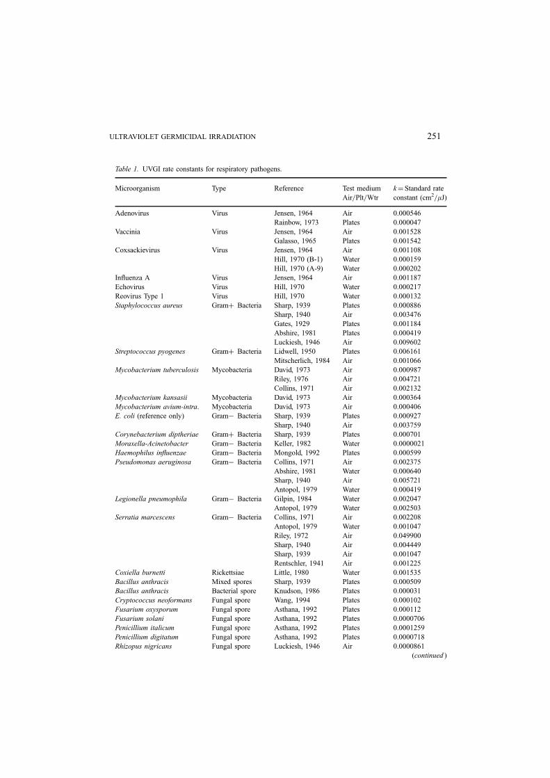
Table 1. UVGI rate constants for respiratory pathogens.

Microorganism Type Reference Test medium

Air=Plt=Wtr

k¼Standard rate

constant (cm2=mJ)

Adenovirus Virus Jensen, 1964 Air 0.000546

Rainbow, 1973 Plates 0.000047

Vaccinia Virus Jensen, 1964 Air 0.001528

Galasso, 1965 Plates 0.001542

Coxsackievirus Virus Jensen, 1964 Air 0.001108

Hill, 1970 (B-1) Water 0.000159

Hill, 1970 (A-9) Water 0.000202

Influenza A Virus Jensen, 1964 Air 0.001187

Echovirus Virus Hill, 1970 Water 0.000217

Reovirus Type 1 Virus Hill, 1970 Water 0.000132

Staphylococcus aureus Gramþ Bacteria Sharp, 1939 Plates 0.000886

Sharp, 1940 Air 0.003476

Gates, 1929 Plates 0.001184

Abshire, 1981 Plates 0.000419

Luckiesh, 1946 Air 0.009602

Streptococcus pyogenes Gramþ Bacteria Lidwell, 1950 Plates 0.006161

Mitscherlich, 1984 Air 0.001066

Mycobacterium tuberculosis Mycobacteria David, 1973 Air 0.000987

Riley, 1976 Air 0.004721

Collins, 1971 Air 0.002132

Mycobacterium kansasii Mycobacteria David, 1973 Air 0.000364

Mycobacterium avium-intra. Mycobacteria David, 1973 Air 0.000406

E. coli (reference only) Gram� Bacteria Sharp, 1939 Plates 0.000927

Sharp, 1940 Air 0.003759

Corynebacterium diptheriae Gramþ Bacteria Sharp, 1939 Plates 0.000701

Moraxella-Acinetobacter Gram� Bacteria Keller, 1982 Water 0.0000021

Haemophilus influenzae Gram� Bacteria Mongold, 1992 Plates 0.000599

Pseudomonas aeruginosa Gram� Bacteria Collins, 1971 Air 0.002375

Abshire, 1981 Water 0.000640

Sharp, 1940 Air 0.005721

Antopol, 1979 Water 0.000419

Legionella pneumophila Gram� Bacteria Gilpin, 1984 Water 0.002047


Serratia marcescens Gram� Bacteria Collins, 1971 Air 0.002208


Riley, 1972 Air 0.049900

Sharp, 1940 Air 0.004449

Sharp, 1939 Air 0.001047

Rentschler, 1941 Air 0.001225

Coxiella burnetti Rickettsiae Little, 1980 Water 0.001535

Bacillus anthracis Mixed spores Sharp, 1939 Plates 0.000509

Bacillus anthracis Bacterial spore Knudson, 1986 Plates 0.000031

Cryptococcus neoformans Fungal spore Wang, 1994 Plates 0.000102

Fusarium oxysporum Fungal spore Asthana, 1992 Plates 0.000112

Fusarium solani Fungal spore Asthana, 1992 Plates 0.0000706

Penicillium italicum Fungal spore Asthana, 1992 Plates 0.0001259

Penicillium digitatum Fungal spore Asthana, 1992 Plates 0.0000718

Rhizopus nigricans Fungal spore Luckiesh, 1946 Air 0.0000861

(continued )

ULTRAVIOLET GERMICIDAL IRRADIATION 251

various media. The wide variation in rate constants predicted reflects the differences in

media, the test arrangements, and the methods of measuring the intensity. In general,

aerosol studies yield moderately higher rate constants than plate studies. This could be

expected since microbes tumbling in the air will receive exposure all around, while

microbes on plates receive exposure in one plane only.

Two-stage survival curves. In general, a small fraction of any microbial population is

resistant to UVGI or other bactericidal factors (Cerf, 1977; Fujikawa and Itoh, 1996).

Typically, over 99% of the microbial population will succumb to initial exposure but a

remaining fraction will survive, sometimes for prolonged periods (Smerage and Teixeira,

1993; Qualls and Johnson, 1983). This effect may be due to clumping (Moats et al., 1971;

Davidovich and Kishchenko, 1991), dormancy (Koch, 1995), or other factors.

The two-stage survival curve can be represented mathematically as the summed

response of two separate microbial populations that have respective rate constants k1

and k2. If we define f as the resistant fraction of the total initial population with rate

constant k2, then ð1 � f Þ is the fraction with rate constant k1. The total survival curve is

therefore the sum of the rapid decay curve (the vulnerable majority) and the slow decay

curve (the resistant minority).

SðtÞ ¼ 1 � fð Þe�k1It þ f e�k2It ð3Þ

where k1¼ rate constant for fast decay population (cm2=mJ), k2¼ rate constant for resistant

population (cm2=mJ), f¼ resistant fraction.

Figure 1 shows data for Streptococcus pyogenes that displays two-stage behavior. The

resistant fraction of most microbial populations may be about 0.01–1% but some studies

suggest it can be a large fraction for certain species (Riley and Kaufman, 1972;

Gates, 1929).

Values of the two-stage rate constants are summarized in Table 2 for the few microbes

for which second stage data has been published. These parameters represent a re-

interpretation of the original published results by the indicated researchers and in all

cases an improved curve-fit resulted. The two-stage rate constants k1 and k2 listed in

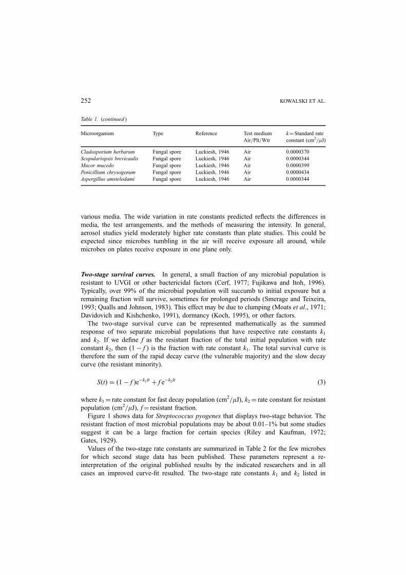
Table 1. (continued )

Microorganism Type Reference Test medium

Air=Plt=Wtr

k¼ Standard rate

constant (cm2=mJ)

Cladosporium herbarum Fungal spore Luckiesh, 1946 Air 0.0000370

Scopulariopsis brevicaulis Fungal spore Luckiesh, 1946 Air 0.0000344

Mucor mucedo Fungal spore Luckiesh, 1946 Air 0.0000399

Penicillium chrysogenum Fungal spore Luckiesh, 1946 Air 0.0000434

Aspergillus amstelodami Fungal spore Luckiesh, 1946 Air 0.0000344

252 KOWALSKI ET AL.

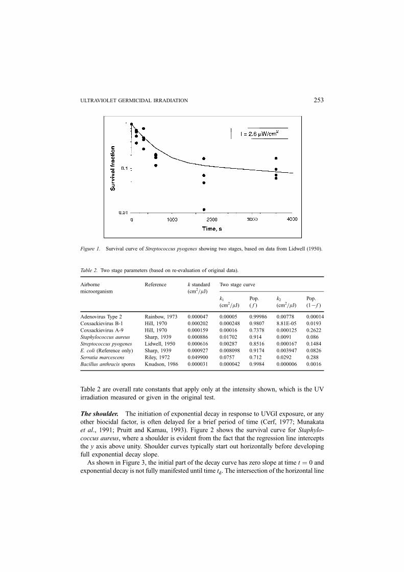
Table 2 are overall rate constants that apply only at the intensity shown, which is the UV

irradiation measured or given in the original test.

The shoulder. The initiation of exponential decay in response to UVGI exposure, or any

other biocidal factor, is often delayed for a brief period of time (Cerf, 1977; Munakata

et al., 1991; Pruitt and Kamau, 1993). Figure 2 shows the survival curve for Staphylo-

coccus aureus, where a shoulder is evident from the fact that the regression line intercepts

the y axis above unity. Shoulder curves typically start out horizontally before developing

full exponential decay slope.

As shown in Figure 3, the initial part of the decay curve has zero slope at time t ¼ 0 and

exponential decay is not fully manifested until time td. The intersection of the horizontal line

Table 2. Two stage parameters (based on re-evaluation of original data).

Airborne

microorganism

Reference k standard

(cm2=mJ)

Two stage curve

k1

(cm2=mJ)

Pop.

( f )

k2

(cm2=mJ)

Pop.

(17f )

Adenovirus Type 2 Rainbow, 1973 0.000047 0.00005 0.99986 0.00778 0.00014

Coxsackievirus B-1 Hill, 1970 0.000202 0.000248 0.9807 8.81E-05 0.0193

Coxsackievirus A-9 Hill, 1970 0.000159 0.00016 0.7378 0.000125 0.2622

Staphylococcus aureus Sharp, 1939 0.000886 0.01702 0.914 0.0091 0.086

Streptococcus pyogenes Lidwell, 1950 0.000616 0.00287 0.8516 0.000167 0.1484

E. coli (Reference only) Sharp, 1939 0.000927 0.008098 0.9174 0.003947 0.0826

Serratia marcescens Riley, 1972 0.049900 0.0757 0.712 0.0292 0.288

Bacillus anthracis spores Knudson, 1986 0.000031 0.000042 0.9984 0.000006 0.0016

Figure 1. Survival curve of Streptococcus pyogenes showing two stages, based on data from Lidwell (1950).


Figure 2. Survival curve of Staphylococcus aureus showing evidence of shoulder (Sharp, 1939).

Figure 3. Development of shoulder curve, showing the effect of the time delay tc and relation to the tangent

point d.

254 KOWALSKI ET AL.

S ¼ 1 (100% Survival) at tc with the extension of the decay curve is known as the ‘‘quasi-

threshold’’ in radiation biology (Casarett, 1968). The point td is tangent to both curves.

The lag in response to the stimulus implies that either a threshold dose is necessary

before measurable effects occur or that repair mechanisms actively deal with low-level

damage (Casarett, 1968). The effect is species and intensity dependent. In many cases it

can be neglected. However, for some species and sometimes for low intensity exposure, the

shoulder can be significant and prolonged.

Recovery due to growth during irradiation is assumed negligible and to be encompassed

by the model—this should be at least partly true if the parameters are based on a broad

range of empirical data. Recovery of spores, although not well understood, is recognized as

a process associated with germination (Russell, 1982). The recovery of spores is, therefore,

a self-limiting factor since a germinated spore invariably becomes less resistant to UVGI

irradiation (Harm, 1980).

An exponential decay curve with a shoulder will have an intercept greater than unity

when the first stage rate constant is extrapolated to the y-axis. It is naturally assumed that a

shoulder exhibited in the data is statistically significant and not an artifact of measurement

uncertainty. Relative to a decay curve that intercepts at unity, the shouldered curve is

shifted ahead by a time interval equal to tc, the quasi-threshold. The equation for the

delayed single stage survival curve, when t � td is:

ln SðtÞ ¼ �kI ðt � tcÞ: ð4Þ

The shoulder occurs during the time interval 0 < t < td. It is apparent that the shoulder

portion is a non-linear function of ln S (see Figure 2). Insufficient data exist to precisely

define the form of the relationship, but ln S cannot be simpler than a polynomial function

of second order. The error resulting from this assumed mathematical relationship will be

small as long as it provides a smooth transition between the horizontal and the delayed

decay curve.

Assuming a second order polynomial relationship between the dose (intensity times

time) and ln S, we have:

ln SðtÞ ¼ �pðItÞ2

ð5Þ

where 0 < t < td, p¼ a constant.

The constant p can be evaluated by requiring continuity through the first derivative

between equations (4) and (5) at the tangent point t ¼ td. For any constant intensity I, the

slope of the exponential portion of the survival curve may be obtained by straightforward

time differentiation of the right hand side of equation (4):

d

dtðln SÞ ¼ �kI ð6Þ


Similarly, the slope of the shoulder curve is obtained by differentiation of the right hand

side of equation (5):

d

dtðln SÞ ¼ �2pI 2t ð7Þ

The constant p is determined by equating (6) and (7) at time td:

p ¼k

2Itdð8Þ

Substitution of this expression for p into equation (5) and equating (6) and (7) at t ¼ tdyields the relation:

td ¼ 2tc ð9Þ

Equation (9) is, in fact, a version of the result Appolonius of Perga arrived at in the 3rd

century BC through lengthy geometry for the special case of ellipses, which are also

described by second order polynomials (Elmer, 1989). The term p is now discarded, after

substituting for equations (8) and (9), and equation (5) can be written in the form:

ln S ¼ �kI

4tct2 ð10Þ

In general, any data set describing single stage microbial decay can be easily fit to a

single stage exponential decay curve. Normally, the y-intercept is fixed at S ¼ 1 when

fitting data to a curve. If a shoulder is suspected, the constraint on the y-intercept should be

removed and the coefficient of the exponential will then have some value greater than 1.

This assumes, of course, that the shoulder is real and not a result of measurement

uncertainty.

The term Si, denotes the y-intercept of the shifted exponential portion of a survival curve

with a shoulder, as shown in Figure 4. If Si is known, the value of tc can be determined by

evaluating equation (4) at t ¼ 0:

tc ¼ln ðSiÞ

kIð11Þ

Note that this mathematical treatment of the shoulder requires transcending the dose

term It since this must be separated into components. The dose may define a point on the

shoulder but the intensity defines the shoulder itself. That is, the threshold tc is a function

of the intensity only, not the dose. Furthermore, in two stage curves there is a separate

shoulder for both stages, although the contribution due to the second stage (the resistant

fraction) is typically small.

256 KOWALSKI ET AL.

The complete single stage survival curve can then be defined as the piecewise

continuous function:

ln SðtÞ ¼�

kI

4tct2; t � 2tc

�kI ðt � tcÞ; t � 2tc

8<: ð12Þ

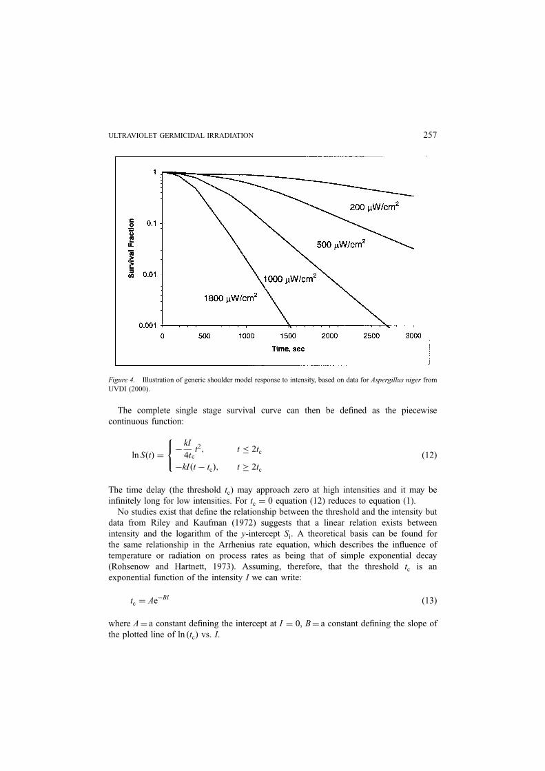
The time delay (the threshold tc) may approach zero at high intensities and it may be

infinitely long for low intensities. For tc ¼ 0 equation (12) reduces to equation (1).

No studies exist that define the relationship between the threshold and the intensity but

data from Riley and Kaufman (1972) suggests that a linear relation exists between

intensity and the logarithm of the y-intercept Si. A theoretical basis can be found for

the same relationship in the Arrhenius rate equation, which describes the influence of

temperature or radiation on process rates as being that of simple exponential decay

(Rohsenow and Hartnett, 1973). Assuming, therefore, that the threshold tc is an

exponential function of the intensity I we can write:

tc ¼ Ae�BI ð13Þ

where A¼ a constant defining the intercept at I ¼ 0, B¼ a constant defining the slope of

the plotted line of ln ðtcÞ vs. I.

Figure 4. Illustration of generic shoulder model response to intensity, based on data for Aspergillus niger from

UVDI (2000).


Given any two sets of data for tc and I, equation (13) can be used to determine the values

of A and B. Prediction of tc for any arbitrary value of intensity I then becomes possible.

Figure 4 shows hypothetical survival curves of spores subject to various intensities.

The complete equation can be defined by combining equation (3) and equation (12),

where a shoulder is considered to be present in both stages:

SðtÞ ¼ f e�k1It0 þ ð1 � f Þe�k2It0 ð14Þ

where

t0 ¼

t2

4tc; t � 2tc

ðt � tcÞ; t � 2tc

8<:

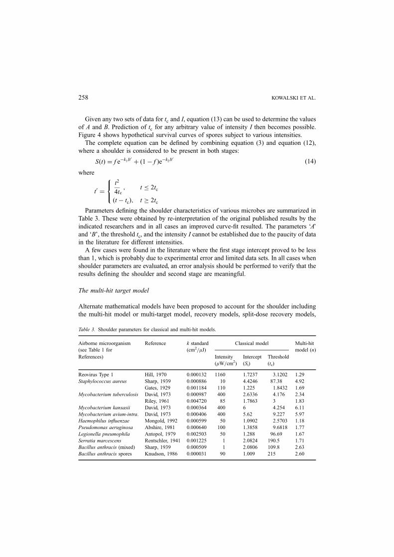
Parameters defining the shoulder characteristics of various microbes are summarized in

Table 3. These were obtained by re-interpretation of the original published results by the

indicated researchers and in all cases an improved curve-fit resulted. The parameters ‘A’

and ‘B’, the threshold tc, and the intensity I cannot be established due to the paucity of data

in the literature for different intensities.

A few cases were found in the literature where the first stage intercept proved to be less

than 1, which is probably due to experimental error and limited data sets. In all cases when

shoulder parameters are evaluated, an error analysis should be performed to verify that the

results defining the shoulder and second stage are meaningful.

The multi-hit target model

Alternate mathematical models have been proposed to account for the shoulder including

the multi-hit model or multi-target model, recovery models, split-dose recovery models,

Table 3. Shoulder parameters for classical and multi-hit models.

Airborne microorganism

(see Table 1 for

Reference k standard

(cm2=mJ)

Classical model Multi-hit

model (n)

References) Intensity

(mW=cm2)

Intercept

(Si)

Threshold

(tc)

Reovirus Type 1 Hill, 1970 0.000132 1160 1.7237 3.1202 1.29

Staphylococcus aureus Sharp, 1939 0.000886 10 4.4246 87.38 4.92

Gates, 1929 0.001184 110 1.225 1.8432 1.69

Mycobacterium tuberculosis David, 1973 0.000987 400 2.6336 4.176 2.34

Riley, 1961 0.004720 85 1.7863 3 1.83

Mycobacterium kansasii David, 1973 0.000364 400 6 4.254 6.11

Mycobacterium avium-intra. David, 1973 0.000406 400 5.62 9.227 5.97

Haemophilus influenzae Mongold, 1992 0.000599 50 1.0902 2.5703 1.18

Pseudomonas aeruginosa Abshire, 1981 0.000640 100 1.3858 9.6818 1.77

Legionella pneumophila Antopol, 1979 0.002503 50 1.288 96.69 1.67

Serratia marcescens Rentschler, 1941 0.001225 1 2.0824 190.5 1.71

Bacillus anthracis (mixed) Sharp, 1939 0.000509 1 2.0806 109.8 2.63

Bacillus anthracis spores Knudson, 1986 0.000031 90 1.009 215 2.60

258 KOWALSKI ET AL.

and empirical models (Russell, 1982; Harm, 1980; Casarett, 1968). The use of the

multi-hit target model, for example, to determine shoulder characteristics is similar in

form to the methods for the classical model (Anellis et al., 1965), and is addressed here for

comparison purposes.

The multi target model (Severin et al., 1983) can be written as follows:

SðtÞ ¼ 1 � 1 � e�kIt� �n

ð15Þ

The parameter n represents the number of discrete critical sites that must be hit to

inactivate the microorganism, and is unique for each species.

In equation (15) the number of targets n must be unique to each population fraction in a

two stage curve, since these behave as though they were independent. Therefore, by

analogy to equation (14) we can write the complete two stage equation for the multi-hit

model as follows:

SðtÞ ¼ ð1 � f Þ 1 � ð1 � e�k1ItÞn1

� �þ f 1 � ð1 � e�k2ItÞ

n2� �

ð16Þ

In equation (16), n1 represents the number of targets for the species in population 1, the

fast decay population, while n2 represents the number of targets in the resistant fraction.

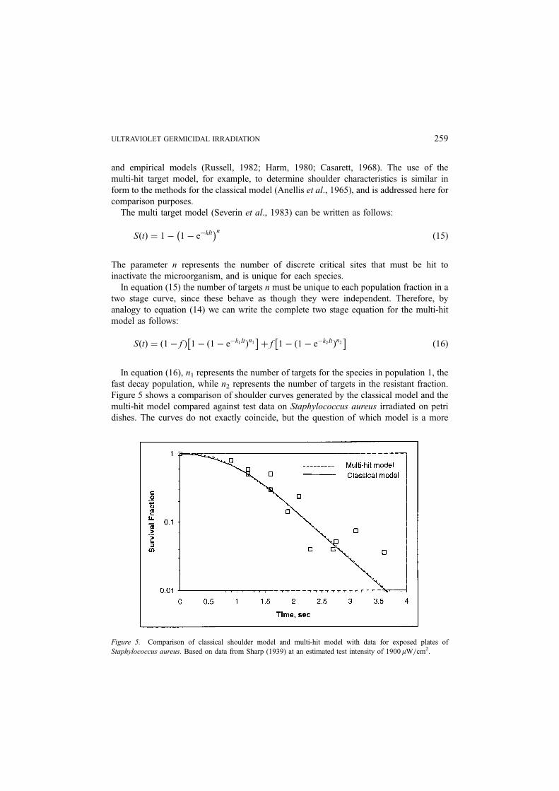
Figure 5 shows a comparison of shoulder curves generated by the classical model and the

multi-hit model compared against test data on Staphylococcus aureus irradiated on petri

dishes. The curves do not exactly coincide, but the question of which model is a more

Figure 5. Comparison of classical shoulder model and multi-hit model with data for exposed plates of

Staphylococcus aureus. Based on data from Sharp (1939) at an estimated test intensity of 1900mW=cm2.


accurate predictor is indeterminate due to experimental error. It remains for future research

to determine which model is a more accurate predictor of shoulder curves. Either model

should suffice for basic analysis and design purposes.

Table 3 includes the value of n, the number of targets, for the multi-hit model which

have been derived from the original test data. These can be used to generate a single stage

shoulder curve similar to the one for the listed shoulder parameters. In all cases the multi-

hit model curve does not exactly coincide with the one produced by the classical model,

yet the error is quite small.

3. Modeling the UV Dose

Two approaches can be taken to define the complete three-dimensional (3D) intensity field

in any experimental apparatus involving airflow—measurement and calculation. Photo-

sensors can provide a profile of the field but they have inherent problems in the near field

(Severin and Roessler, 1998) and have difficulties when used inside reflective enclosures.

The question of whether photosensors can be used to measure the fluence rate that an

airborne microbe actually experiences is an unresolved one. Recent advances in the use of

spherical actinometry (Rahn et al., 1999) may provide more realistic results since these

sensors more closely resemble spherical microbes.

The problems of photosensing and data interpretation can be avoided through analytical

determination of the 3D intensity field. The use of radiation view factors to define the 3D

intensity field for both the lamp and internal reflective surfaces has been detailed by

Kowalski and Bahnfleth (2000) and is summarized here.

Various models of the intensity field due to UV lamps have been proposed in the past,

including point source, line source, integrated line source, and other models (Jacob and

Dranoff, 1970; Qualls and Johnson, 1983; Beggs et al., 2000). The model used here is

based on thermal radiation view factors (Modest, 1993), which define the amount of

diffuse radiation transmitted from one surface to another.

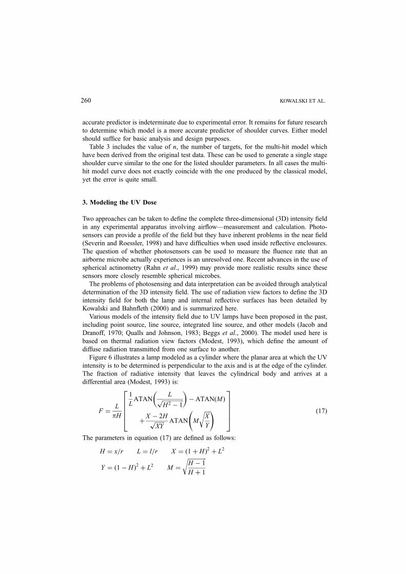
Figure 6 illustrates a lamp modeled as a cylinder where the planar area at which the UV

intensity is to be determined is perpendicular to the axis and is at the edge of the cylinder.

The fraction of radiative intensity that leaves the cylindrical body and arrives at a

differential area (Modest, 1993) is:

F ¼L

pH

1

LATAN

LffiffiffiffiffiffiffiffiffiffiffiffiffiffiffiH2 � 1

p

� ATANðM Þ

þX � 2Hffiffiffiffiffiffiffi

XYp ATAN M

ffiffiffiffiX

Y

r !266664

377775 ð17Þ

The parameters in equation (17) are defined as follows:

H ¼ x=r L ¼ l=r X ¼ ð1 þ HÞ2þ L2

Y ¼ ð1 � HÞ2þ L2 M ¼

ffiffiffiffiffiffiffiffiffiffiffiffiffiH � 1

H þ 1

r

260 KOWALSKI ET AL.

where l¼ length of the lamp segment (arclength, cm), x¼ distance from the lamp (cm),

r¼ radius of the lamp (cm).

This equation applies to a differential element located at the edge of the lamp segment. In

order to compute the view factor at any point along a lamp it must be divided into two

segments. Equation (17) can be used to compute the intensity at any point beyond the ends of

the lamp by applying it twice—once to compute the view factor for an imaginary lamp of the

total length (distance between some point and the far end of the lamp) and then subtracting

the view factor of the non-existent portion, or ghost portion. This method, known as view

factor algebra, is detailed in Kowalski and Bahnfleth (2000) and elsewhere (Modest, 1993).

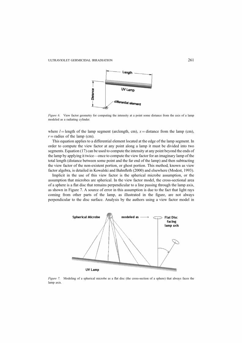
Implicit in the use of this view factor is the spherical microbe assumption, or the

assumption that microbes are spherical. In the view factor model, the cross-sectional area

of a sphere is a flat disc that remains perpendicular to a line passing through the lamp axis,

as shown in Figure 7. A source of error in this assumption is due to the fact that light rays

coming from other parts of the lamp, as illustrated in the figure, are not always

perpendicular to the disc surface. Analysis by the authors using a view factor model in

Figure 6. View factor geometry for computing the intensity at a point some distance from the axis of a lamp

modeled as a radiating cylinder.

Figure 7. Modeling of a spherical microbe as a flat disc (the cross-section of a sphere) that always faces the

lamp axis.


which the intensity has been corrected for the cosines of the angles from non-perpendi-

cular rays has established that this difference is quite small and can be neglected in most

cases. This is due to the fact that when the disc element is close to the lamp surface the

nearest sections of the lamp dominate the intensity field, while at large distances the

cosines become small.

The intensity field as a function of distance from the lamp axis is simply the product of

the surface intensity and the view factor, where the surface intensity is computed by

dividing the UV power output by the surface area of the lamp:

I ¼Euv

2prlFtotal ð18Þ

where Euv ¼UV power output of lamp, mW.

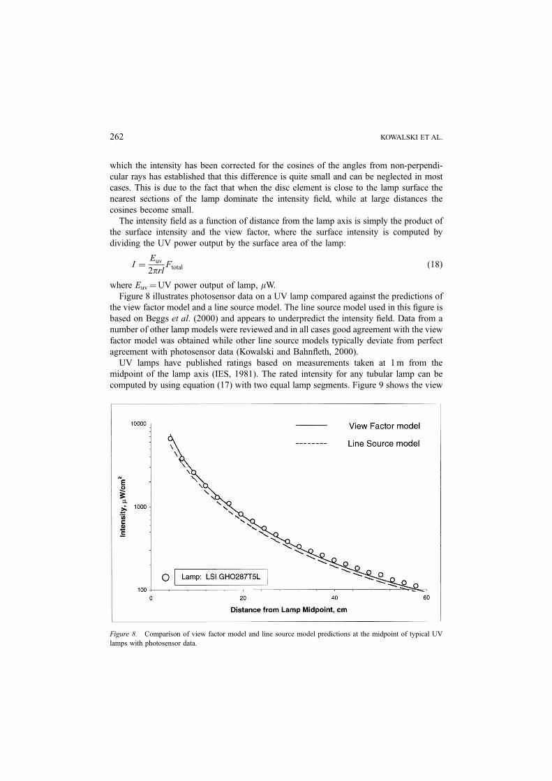
Figure 8 illustrates photosensor data on a UV lamp compared against the predictions of

the view factor model and a line source model. The line source model used in this figure is

based on Beggs et al. (2000) and appears to underpredict the intensity field. Data from a

number of other lamp models were reviewed and in all cases good agreement with the view

factor model was obtained while other line source models typically deviate from perfect

agreement with photosensor data (Kowalski and Bahnfleth, 2000).

UV lamps have published ratings based on measurements taken at 1 m from the

midpoint of the lamp axis (IES, 1981). The rated intensity for any tubular lamp can be

computed by using equation (17) with two equal lamp segments. Figure 9 shows the view

Figure 8. Comparison of view factor model and line source model predictions at the midpoint of typical UV

lamps with photosensor data.

262 KOWALSKI ET AL.

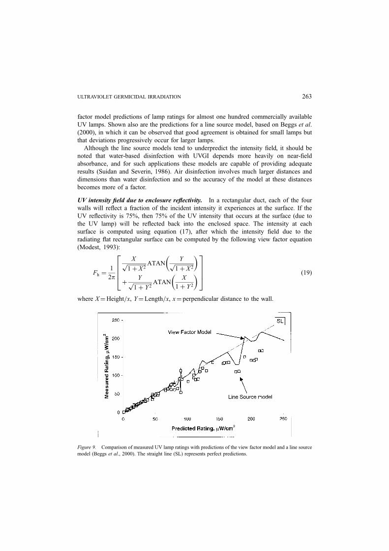
factor model predictions of lamp ratings for almost one hundred commercially available

UV lamps. Shown also are the predictions for a line source model, based on Beggs et al.

(2000), in which it can be observed that good agreement is obtained for small lamps but

that deviations progressively occur for larger lamps.

Although the line source models tend to underpredict the intensity field, it should be

noted that water-based disinfection with UVGI depends more heavily on near-field

absorbance, and for such applications these models are capable of providing adequate

results (Suidan and Severin, 1986). Air disinfection involves much larger distances and

dimensions than water disinfection and so the accuracy of the model at these distances

becomes more of a factor.

UV intensity field due to enclosure reflectivity. In a rectangular duct, each of the four

walls will reflect a fraction of the incident intensity it experiences at the surface. If the

UV reflectivity is 75%, then 75% of the UV intensity that occurs at the surface (due to

the UV lamp) will be reflected back into the enclosed space. The intensity at each

surface is computed using equation (17), after which the intensity field due to the

radiating flat rectangular surface can be computed by the following view factor equation

(Modest, 1993):

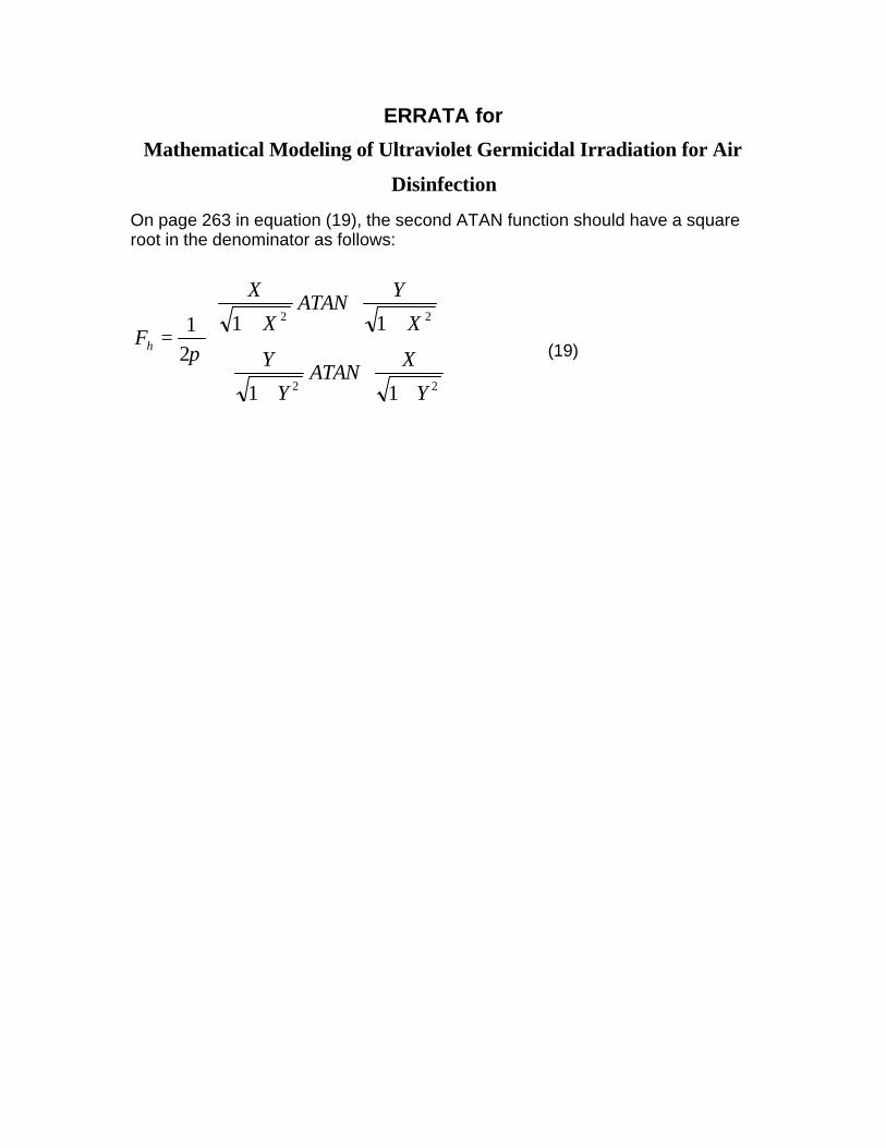
Fh ¼1

2p

Xffiffiffiffiffiffiffiffiffiffiffiffiffiffi1 þ X 2

p ATANYffiffiffiffiffiffiffiffiffiffiffiffiffiffi

1 þ X 2p

þYffiffiffiffiffiffiffiffiffiffiffiffiffiffi

1 þ Y 2p ATAN

X

1 þ Y 2

26664

37775 ð19Þ

where X¼Height=x, Y¼Length=x, x¼ perpendicular distance to the wall.

Figure 9. Comparison of measured UV lamp ratings with predictions of the view factor model and a line source

model (Beggs et al., 2000). The straight line (SL) represents perfect predictions.


This view factor is consistent with the previously stated spherical microbe assumption in

that equation (19) is applied to all four walls as if the microbe faced each one individually.

The intensity field due to each surface is then summed to obtain the total reflected intensity

field. The error due to the fact that some portions of the rectangular surface are not

perpendicular to the flat disc element that represents the spherical microbe is negligible for

the same reasons discussed previously. In addition, the distances to the walls are, in general

greater, and the surface intensities lower, rendering the error still more negligible.

Subsequent reflections, called inter-reflections, can be accounted for with more

sophisticated computational methods (Kowalski and Bahnfleth, 2000; Kowalski, 2001),

but equation (19) may suffice as a reasonable first order approximation if the material has

low reflectivity.

Rate constant determination. Previously, no analytical method existed to enable

researchers to accurately evaluate the intensity field and assess the dose received by

airborne microbes in experimental setups. As a result, airborne rate constants could not

easily be determined. In some airborne experiments the airstream was confined to an area

of known intensity by directing airflow through a narrow slot (Riley and Kaufman, 1972).

Given the methods and analytical tools described above, airborne rate constants can now be

determined with improved accuracy. As mentioned previously, rate constants depend on the

test apparatus and measurement methods and so are relative to the experiment from which

they come. The analytical methods presented here enable easy resolution of the intensity field

and can readily predict rate constants, but with the caveat that these rate constants are, in turn,

dependent on these methods. That is to say, an airborne rate constant determined with the

present methods can be used for predictive purposes, but only if these methods are also used

for the predictions. Otherwise, what certainty there is in the prediction would be diminished.

4. Air Mixing Effects

In long ducts the velocity profile of a laminar airstream will approach a parabolic shape,

with the velocity higher towards the center. However, fully developed laminar velocity

profiles are unlikely to be achieved in laboratory or real-world installations. The design

velocity of a typical UVGI system is about 2.54 m=s (500 fpm), producing a Reynolds

number of approximately 150,000. Turbulent mixing is therefore more likely to be the

norm. Even laminar flow involves mixing by diffusion and so actual operating conditions

will lie somewhere between complete mixing and the idealized condition of completely

unmixed flow. Real world conditions tend to approach those of complete mixing, and such

was shown by Severin et al. (1984) for water-based systems.

These bounding conditions, complete mixing and unmixed flow, assume a flat velocity

profile. Rate constants due to the latter are computed using the average intensity. The total

survival, for each stage if there are two stages in the survival curve, is as follows:

S ¼ e�kIavgt ð20Þ

where Iavg ¼ average intensity in the irradiation chamber (mW=cm2).

264 KOWALSKI ET AL.

The average intensity can be computed for any irradiation chamber using equations (17)

and (19) with a 3D matrix of sufficient resolution. A computer model developed by the

authors uses a matrix of 50 50 100 with satisfactory results.

If the airflow through a UVGI chamber followed perfectly parallel streamlines without

mixing then each streamline will produce a unique dose that depends on the distance from

the lamp. The survival rate in this case must be calculated for each streamline segment and

summed or ‘integrated’ to obtain the net survival. The survival Si for each streamline

segment is computed by equation (20) and the total survival would be the sum of all

streamline segments as follows:

S ¼Xl

j¼1

Xm

i¼1

Xn

k¼1

e�kIijk t ð21Þ

where Iijk ¼ Intensity at point ijk, i¼ a point defining the x coordinate (width), j¼ a point

defining the y coordinate (height), k¼ a point defining the z coordinate (length),

t¼ exposure time for each segment defined by point ijk.

The exposure time is constant for each streamline segment. The population is assumed

to be equally divided among all streamlines in the flat velocity profile. In the event the

velocity profile is known and is not flat, the exposure time in equation (21) can be indexed

to account for the actual velocities.

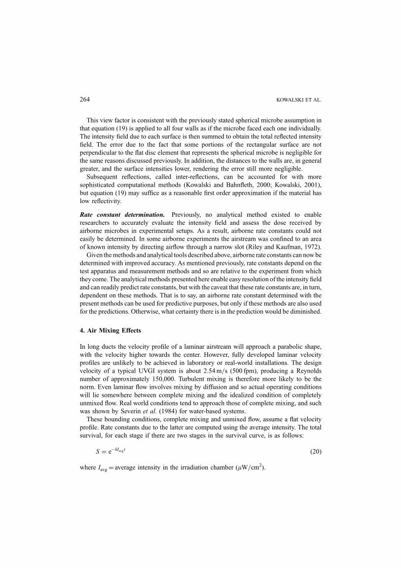
Equation (21) permits the development of a contour map of the ‘kill zones’ of the

unmixed condition for any UVGI system configuration. Consider two typical systems as

shown in Figure 10a, which is commonly known as crossflow, and Figure 10b which is

called axial flow. The kill zones developed from the above methodology, as implemented

by the authors’ software, are shown in Figure 11a and 11b for a single lamp system in a

57% reflective chamber and Serratia marcescens as the test microbe.

In Figure 11a, for the crossflow condition, the kill rate was predicted to be 59–64%,

where 59% represents unmixed and 64% the mixed air conditions. In Figure 11b, using

the same 5.5 watt lamp in the axial flow case, the range of kill rates was predicted to be

53–56%.

Figure l0a, b. Schematic of crossflow and axial flow configurations.


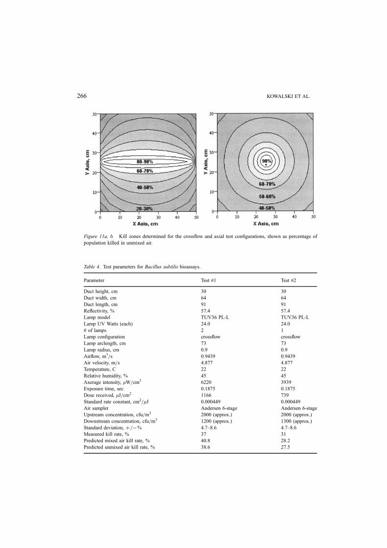
Figure 11a, b. Kill zones determined for the crossflow and axial test configurations, shown as percentage of

population killed in unmixed air.

Table 4. Test parameters for Bacillus subtilis bioassays.

Parameter Test #1 Test #2

Duct height, cm 30 30

Duct width, cm 64 64

Duct length, cm 91 91

Reflectivity, % 57.4 57.4

Lamp model TUV36 PL-L TUV36 PL-L

Lamp UV Watts (each) 24.0 24.0

# of lamps 2 1

Lamp configuration crossflow crossflow

Lamp arclength, cm 73 73

Lamp radius, cm 0.9 0.9

Airflow, m3=s 0.9439 0.9439

Air velocity, m=s 4.877 4.877

Temperature, C 22 22

Relative humidity, % 45 45

Axerage intensity, mW=cm2 6220 3939

Exposure time, sec 0.1875 0.1875

Dose received, mJ=cm2 1166 739

Standard rate constant, cm2=mJ 0.000449 0.000449

Air sampler Andersen 6-stage Andersen 6-stage

Upstream concentration, cfu=m3 2000 (approx.) 2000 (approx.)

Downstream concentration, cfu=m3 1200 (approx.) 1300 (approx.)

Standard deviation, þ=�% 4.7–8.6 4.7–8.6

Measured kill rate, % 37 31

Predicted mixed air kill rate, % 40.8 28.2

Predicted unmixed air kill rate, % 38.6 27.5

266 KOWALSKI ET AL.

The computer program developed by the authors can resolve the intensity field for any

reflective rectangular enclosure, which can then be used to determine airborne rate

constants from bioassays. This program has been used to interpret test data from over

twenty laboratory tests to determine the airborne rate constant for Serratia marcescens,

which has been found to be approximately 0.00291 cm2=mJ (Kowalski and Bahnfleth,

2000).

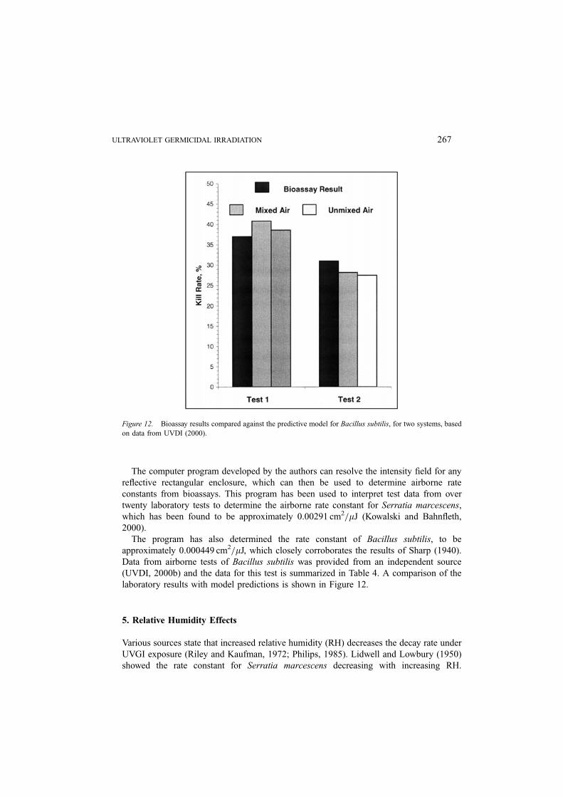
The program has also determined the rate constant of Bacillus subtilis, to be

approximately 0.000449 cm2=mJ, which closely corroborates the results of Sharp (1940).

Data from airborne tests of Bacillus subtilis was provided from an independent source

(UVDI, 2000b) and the data for this test is summarized in Table 4. A comparison of the

laboratory results with model predictions is shown in Figure 12.

5. Relative Humidity Effects

Various sources state that increased relative humidity (RH) decreases the decay rate under

UVGI exposure (Riley and Kaufman, 1972; Philips, 1985). Lidwell and Lowbury (1950)

showed the rate constant for Serratia marcescens decreasing with increasing RH.

Figure 12. Bioassay results compared against the predictive model for Bacillus subtilis, for two systems, based

on data from UVDI (2000).


Rentschler and Nagy (1942) showed the rate constant for Streptococcus pyogenes

increasing with increasing RH.

These results suggest that the relationship between RH and UVGI susceptibility is at least

species-dependent and therefore no definitive general relationship can be established at

present. Furthermore, no RH study can be performed without aerosolizing microorganisms

and this requires more detailed treatment of the 3D intensity field than has previously been

accomplished. Since RH impacts the measured rate constant, tests on the impact of RH are

essentially measurements of the rate constant and can be given the same analytical treatment.

6. Sources of Predictive Error

Several sources may contribute errors to the predictions of the view factor model,

including the error in the lamp wattage, variations in local voltage, errors in the

photosensor readings, and variations of surface intensity along the lamp. The rate constant

itself is subject to some level of microbiological uncertainty.

A comparison of predicted ratings using the view factor model for over 90 different

UVGI lamp indicates predictive errors within �9% (Kowalski and Bahnfleth, 2000). This

assumes that the ratings are accurate, but there are likely to be inherent errors in the

published ratings as well as the nominal UV power.

According to Severin and Roessler (1998) the largest error in the lamp photosensor is

due to the setback of the sensor inside the body of the photosensor, or an error of 1 cm in

the distance to the source. Additionally, readings cannot be taken at distances defined more

accurately than about 0.1 cm. Finally, the photosensor itself has some inherent error.

The UV power output and lamp rating specified for UVGI lamps may vary. Manu-

facturers typically state the error in the nominal UV wattage is �1% but this may be

optimistic. Blatchley (1997) measured wattage variations in the same model lamp of

þ3.7%=�2.2%. These variations and uncertainties point out the need for improved

methods of verifying lamp power.

Measurements should either be taken of all parameters that could affect the predictive

accuracy of the model, including lamp wattage, line voltage, and the reflectivity of

surfaces, or else the lamp intensity field itself should be corroborated with measurements.

7. Results and Discussion

A comprehensive mathematical model of UVGI disinfection has been presented which

includes a new model for the shoulder portion of the survival curve. A model for the 3D

intensity field of a UVGI system has been summarized that offers investigators the

possibility of extracting rate constants from tests on aerosolized microorganisms.

Airborne rate constants have been determined or corroborated using these models for

Serratia marcescens and Bacillus subtilis. Table 2 summarizes parameters for two stage

decay curves and Table 3 summarizes shoulder parameters based on re-analysis of

published test data.

268 KOWALSKI ET AL.

The problem of air mixing in conjunction with the 3D intensity field has been addressed

by establishing bounds or error limits within which investigators can determine UVGI rate

constants in aerosol based studies.

The methods and equations presented here will enable microbiologists to accurately

interpret aerosol studies on UVGI disinfection and to design better experiments. Since

studies on relative humidity effects require the use of aerosols the methods presented here

will facilitate the resolution of the humidity effects question. The authors have developed

software for this purpose and can provide interpretation of experimental results for

researchers conducting such experiments.

The authors hope that this information will stimulate new studies of UVGI disinfection,

especially in relation to the determination of UVGI rate constants for all airborne

pathogens and the study of relative humidity effects on rate constants. The resolution of

the rate constants for all airborne pathogens will greatly assist the design of new, more

effective systems for the control of airborne disease.

References

R.L. Abshire, H. Dunton, Applied and Environmental Microbiology 41, 1419–1423 (1981).

A. Anellis, N. Grecz, D. Berkowitz, Applied Microbiology 13, 397–401 (1965).

S.C. Antopol, P.D. Ellner, Applied and Environmental Microbiology 38, 347–348 (1979).

A. Asthana, R.W. Tuveson, International Journal of Plant Science 153, 442–452 (1992).

C.B. Beggs, K.G. Kerr, J.K. Donelly, P.A. Sleigh, D.D. Mara, G. Cairns, Transactions of the Royal Society of

Tropical Medicine and Hygiene 94, 141–146 (2000).

E.F. Blatchley, Water Research 31, 2205–2218 (1997).

A.P. Casarett, Radiation Biology (Prentice-Hall, Englewood, 1968).

O. Cerf, Journal of Applied Bacteriology 42, 1–19 (1977).

H. Chick, Journal of Hygiene 8, 92 (1908).

F.M. Collins, Applied Microbiology 21, 411–413 (1971).

H.L. David, The American Review of Respiratory Disease 108, 1175–1184 (1973).

I.A. Davidovich, G.P. Kishchenko, Molecular Genetics, Microbiology and Virology 6, 13–16 (1991).

W.B. Elmer, The Optical Design of Reflectors (TLA Lighting Consultants, Inc., Salem, MA, 1989).

H. Fujikawa, T. Itoh, Applied Microbiology 62, 3745–3749 (1996).

G.J. Galasso, D.G. Sharp, Journal of Bacteriology 90, 1138–1142 (1965).

F.L. Gates, Journal of General Physiology 13, 231–260 (1929).

R.W. Gilpin, in Legionella: Proceedings of the 2nd International Symposium, edited by C. Thornsberry

(American Society for Microbiology, Washington, 1984).

W. Harm, Biological Effects of Ultraviolet Radiation (Cambridge University Press, New York, 1980)

W.F. Hill, F.E. Hamblet, W.H. Benton, E.W. Akin, Applied Microbiology 19, 805–812 (1970).

IES, Lighting Handbook Application Volume (Illumination Engineering Society, 1970).

S.M. Jacob, J.S. Dranoff, AIChE Journal 16, 359–363 (1970).

M.M. Jensen, Applied Microbiology 12, 418–420 (1964).

L.C. Keller, T.L. Thompson, R.B. Macy Applied and Environmental Microbiology 43, 424–429 (1982).

G.B. Knudson, Applied and Environmental Microbiology 52, 444–449 (1986).

A.L. Koch, Bacterial Growth and Form (Chapman & Hall, New York, 1995).

W.J. Kowalski, W.P. Bahnfleth, ASHRAE Transactions 106, 4–15 (2000).

W.J. Kowalski, PhD Thesis, The Pennsylvania State University (2001).

O.M. Lidwell, E.J. Lowbury, Annual Review of Microbiology 14, 38–43 (1950).

J.S. Little, R.A. Kishimoto, P.G. Canonico, Infection Immunity 27, 837–841 (1980).


M. Luckiesh, Applications of Germicidal, Erythemal and Infrared Energy (D. Van Nostrand Co., New York, 1946).

E. Mitscherlich, E.H. Marth, Microbial Survival in the Environment (Springer-Verlag, Berlin, 1984).

W.A. Moats, R. Dabbah, V.M. Edwards, Journal of Food Science 36, 523–526 (1971).

M.F. Modest, Radiative Heat Transfer (McGraw-Hill, New York, 1993).

J. Mongold, Genetics 132, 893–898 (1992).

N. Munakata, M. Saito, K. Hieda, Photochemistry and Photobiology 54, 761–768 (1991).

Philips, Germicidal Lamps and Applications (Catalog No. U.D.C. 628.9, Netherlands, 1985).

K.M. Pruitt, D.N. Kamau, Journal of Industrial Microbiology 12, 221–231 (1993).

R.G. Qualls, J.D. Johnson, Applied Microbiology 45, 872–877 (1983).

R.O. Rahn, P. Xu, S.L. Miller. Photochemistry and Photobiology 70, 314–318 (1999).

A.J. Rainbow, S. Mak, International Journal of Radiation Biology 24, 59–72 (1973).

H.C. Rentschler, R. Nagy, G. Mouromseff, Journal of Bacteriology 42, 745–774 (1941).

H.C. Rentschler, R. Nagy, Journal of Bacteriology 44, 85–94 (1942).

R.L. Riley, M. Knight, G. Middlebrook, American Review of Respiratory Disease 113, 413–418 (1976).

R.L. Riley, J.E. Kaufman, Applied Microbiology 23, 1113–1120 (1972).

W.M. Rohsenow, J.P. Hartnett, Handbook of Heat Transfer (McGraw-Hill, New York, 1973).

A.D. Russell, The Destruction of Bacterial Spores (Academic Press, New York, 1982).

B.F. Severin, M.T. Suidan, R.S. Englebrecht, Water Research 17, 1669–1678 (1983).

B.F. Severin, M.T. Suidan, B.E. Rittmann, R.S. Englebrecht, Journal of Water Pollution Control 56, 164–169

(1984).

B.F. Severin, P.F. Roessler, Water Research 32, 1718–1724 (1998).

G. Sharp, Journal of Bacteriology 37, 447–459 (1939).

G. Sharp, Journal of Bacteriology 38, 535–547 (1940).

G.H. Smerage, A.A. Teixeira, Journal of Industrial Microbiology 12, 211–220 (1993).

M.T. Suidan, B.F. Severin, AIChE Journal 32, 1902–1909 (1986).

UVDI, Report on Bioassays of S. marscecens and B. subtilis exposed to UV irradiation. Ultraviolet Devices, Inc.

(2000).

Y. Wang, A. Casadevall, Applied Microbiology 60, 3864–3866 (1994).

270 KOWALSKI ET AL.

ERRATA for

Mathematical Modeling of Ultraviolet Germicidal Irradiation for Air

Disinfection

On page 263 in equation (19), the second ATAN function should have a square root in the denominator as follows:

+++

++=

22

22

11

1121

Y

XATAN

Y

Y

X

YATAN

X

X

Fh π (19)

Mathematical Modeling of Ultraviolet Germicidal ... · Mathematical Modeling of Ultraviolet...

Documents

Transcript of Mathematical Modeling of Ultraviolet Germicidal ... · Mathematical Modeling of Ultraviolet...