MATHEMATICAL MODELING OF MATERIALLY NONLINEAR PROBLEMS · PDF fileMATHEMATICAL MODELING OF...

FACTA UNIVERSITATIS Series: Architecture and Civil Engineering Vol. 8, No 1, 2010, pp. 67 - 78 DOI: 10.2298/FUACE1001067B

MATHEMATICAL MODELING OF MATERIALLY NONLINEAR PROBLEMS IN STRUCTURAL ANALYSES

(I PART – THEORETICAL FUNDAMENTALS)

UDC 624.131:539.32+539.374+539:57(045)=111

Zoran Bonić, Verka Prolović, Biljana Mladenović

Faculty of Civil Engineering and Architecture, Aleksandra Medvedeva 14, 18000 Niš, Serbia E-mail: [email protected]

Abstract. Material models describe the way they behave when loaded. The paper presents the development of the model beginning with the simplest linear-elastic and rigid-plastic ones. The basic data in the plasticity theory have been defined, such as criterion and yield (failure) surface, hardening law, plastic yield law and normality condition. Yield criteria of Tresca, Von Mises, Mohr-Coulomb and Drucker-Prager were given separately.

Key words: material models, plasticity, yield criterion, yield surface.

1. INTRODUCTION In order to describe behavior of a material in a suitable way, it is necessary to establish

constitutive models (constitutive relations or equations) representing mathematical descrip-tions of their behavior under external load. The constitutive models are formed by estab-lishing relationship between the stress tensor and strain tensor and represent an idealized, that is, more or less rough description of real behavior. Two most frequently applied basic models, describing material properties are ideally-elastic and ideally-plastic models. Real materials almost never meet the conditions defined by the terms for the given models, but they were, primarily due to their simplicity, indispensable for professional practice. In the recent period, with the advent and development of the plasticity theory, new elasto-plastic models have emerged, much more realistically describing the non-linear characteristics of various granular (friction) materials, such as concrete, soil and rock in civil engineering.

Chronologically speaking, elastic models were the first established models of material behavior. The materials described by this model deform under the action of external forces, and after the termination of the action they assume their original shape. Deforma-tions are reversible, relation of stress and strain is unequivocal, that is, stress state is only a function of the strain state and is independent of the stress path.

Received May, 2010

Z. BONIĆ, V. PROLOVIĆ, B. MLADENOVIĆ 68

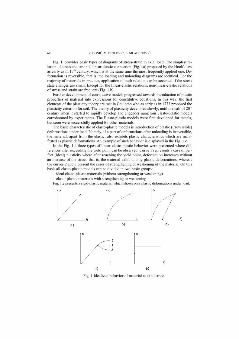
Fig. 1. provides basic types of diagrams of stress-strain in axial load. The simplest re-lation of stress and strain is linear elastic connection (Fig.1.a) proposed by the Hook's law as early as in 17th century, which is at the same time the most frequently applied one. De-formation is reversible, that is, the loading and unloading diagrams are identical. For the majority of materials in practice, application of such relation can be accepted if the stress state changes are small. Except for the linear-elastic relations, non-linear-elastic relations of stress and strain are frequent (Fig. 1.b)

Further development of constitutive models progressed towards introduction of plastic properties of material into expressions for constitutive equations. In this way, the first elements of the plasticity theory are met in Coulomb who as early as in 1773 proposed the plasticity criterion for soil. The theory of plasticity developed slowly, until the half of 20th century when it started to rapidly develop and engender numerous elasto-plastic models corroborated by experiments. The Elasto-plastic models were first developed for metals, but soon were successfully applied for other materials.

The basic characteristic of elasto-plastic models is introduction of plastic (irreversible) deformations under load. Namely, if a part of deformations after unloading is irreversible, the material, apart from the elastic, also exhibits plastic characteristics which are mani-fested as plastic deformations. An example of such behavior is displayed in the Fig. 1.c.

In the Fig. 1.d three types of linear elasto-plastic behavior were presented where dif-ferences after exceeding the yield point can be observed. Curve 1 represents a case of per-fect (ideal) plasticity where after reaching the yield point, deformation increases without an increase of the stress, that is, the material exhibits only plastic deformations, whereas the curves 2 and 3 present the cases of strengthening of weakening of the material. On this basis all elasto-plastic models can be divided in two basic groups:

− ideal elasto-plastic materials (without strengthening or weakening) − elasto-plastic materials with strengthening or weakening Fig. 1.e presents a rigid-plastic material which shows only plastic deformations under load.

Fig. 1 Idealized behavior of material at axial stress

Mathematical Modeling of Materially Nonlinear Problems in Structural Analyses ... 69

2. BASIC CONCEPTS OF PLASTICITY THEORY

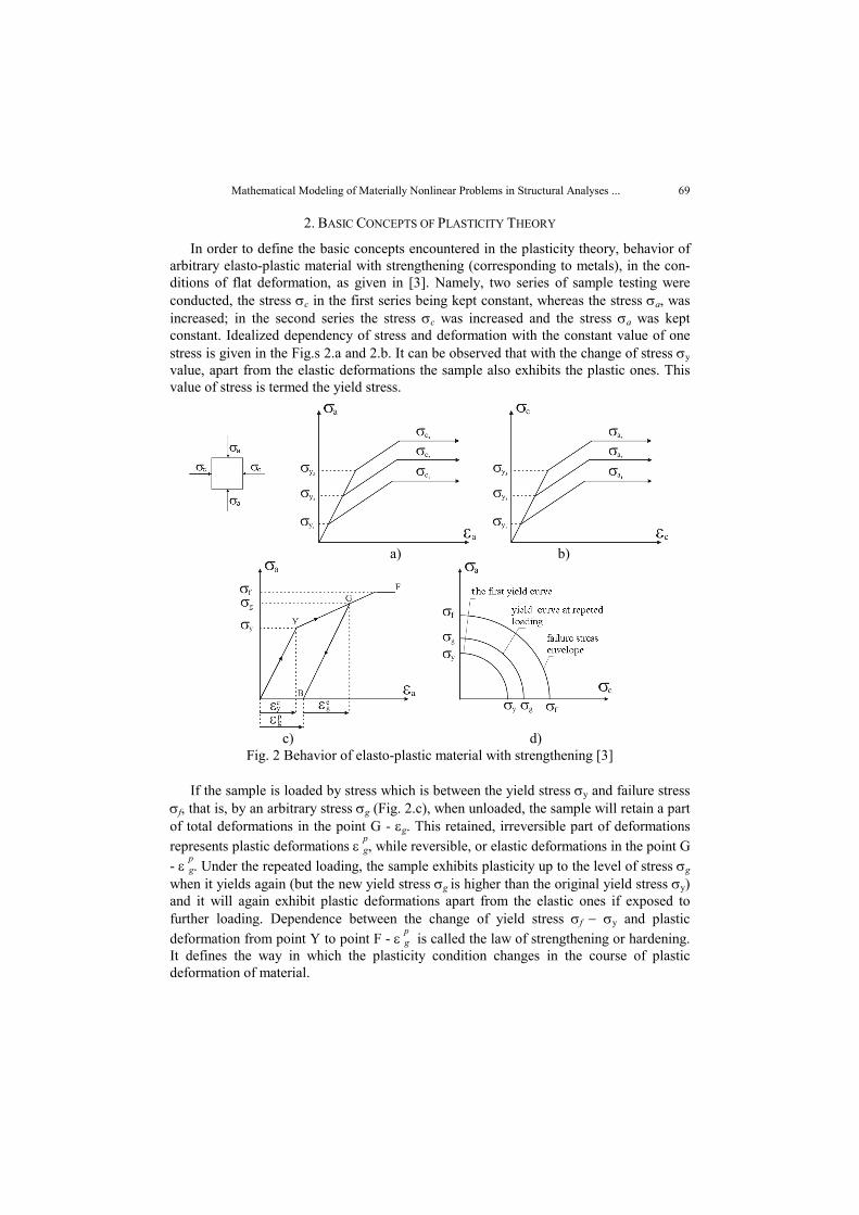
In order to define the basic concepts encountered in the plasticity theory, behavior of arbitrary elasto-plastic material with strengthening (corresponding to metals), in the con-ditions of flat deformation, as given in [3]. Namely, two series of sample testing were conducted, the stress σc in the first series being kept constant, whereas the stress σa, was increased; in the second series the stress σc was increased and the stress σa was kept constant. Idealized dependency of stress and deformation with the constant value of one stress is given in the Fig.s 2.a and 2.b. It can be observed that with the change of stress σy value, apart from the elastic deformations the sample also exhibits the plastic ones. This value of stress is termed the yield stress.

a) b)

c) d)

Fig. 2 Behavior of elasto-plastic material with strengthening [3]

If the sample is loaded by stress which is between the yield stress σy and failure stress σf, that is, by an arbitrary stress σg (Fig. 2.c), when unloaded, the sample will retain a part of total deformations in the point G - εg. This retained, irreversible part of deformations represents plastic deformations ε pg, while reversible, or elastic deformations in the point G - ε pg. Under the repeated loading, the sample exhibits plasticity up to the level of stress σg when it yields again (but the new yield stress σg is higher than the original yield stress σy) and it will again exhibit plastic deformations apart from the elastic ones if exposed to further loading. Dependence between the change of yield stress σf − σy and plastic deformation from point Y to point F - ε pg is called the law of strengthening or hardening. It defines the way in which the plasticity condition changes in the course of plastic deformation of material.


Elasto-plastic behavior of material can be presented in the diagram σa−σc in Fig. 2.d where all the combinations of stresses σa and σc, where the first yield occurs, are pre-sented by the yield line. All combinations of stresses σa and σc when material fails are presented by the failure stress envelope. Unloading, then repeated loading in the point G is presented by the line σg−σg. There is an infinite number of such lines between the first yield line σy−σy and failure line σf−σf and they form a yield surface between the first yield curve and failure envelope. Therefore if the combination of stresses is such that the point is below the yield line, the specimen will behave elastically, when it is in the yield surface the specimen will exhibit both elastic and plastic deformations, and when it reaches the failure stress envelope, it either experience brittle failure or is plastically deformed without elastic deformations. Outside the stress failure envelope, there are impossible stress states. One should take note the failure stress envelope can be, but need not be, geometrically similar to the failure curves.

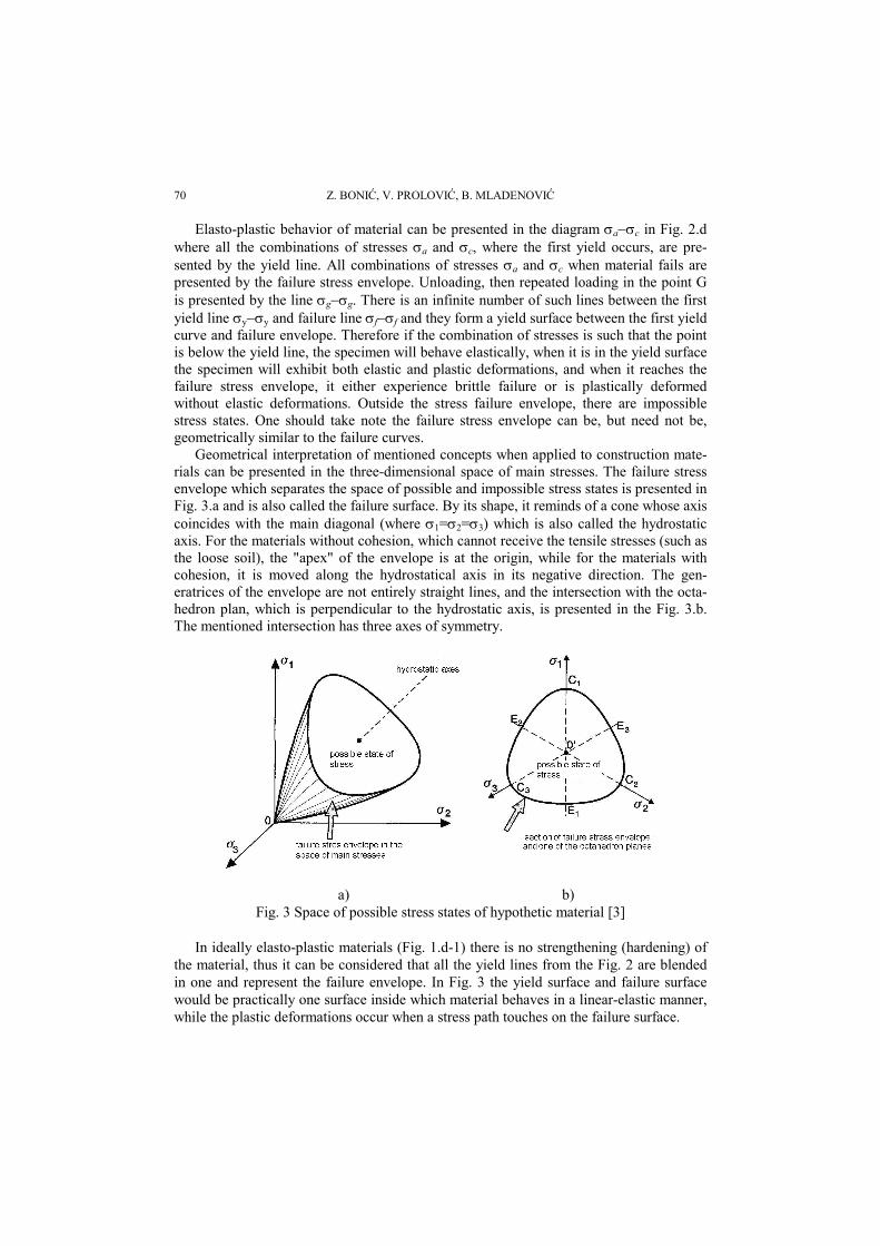
Geometrical interpretation of mentioned concepts when applied to construction mate-rials can be presented in the three-dimensional space of main stresses. The failure stress envelope which separates the space of possible and impossible stress states is presented in Fig. 3.a and is also called the failure surface. By its shape, it reminds of a cone whose axis coincides with the main diagonal (where σ1=σ2=σ3) which is also called the hydrostatic axis. For the materials without cohesion, which cannot receive the tensile stresses (such as the loose soil), the "apex" of the envelope is at the origin, while for the materials with cohesion, it is moved along the hydrostatical axis in its negative direction. The gen-eratrices of the envelope are not entirely straight lines, and the intersection with the octa-hedron plan, which is perpendicular to the hydrostatic axis, is presented in the Fig. 3.b. The mentioned intersection has three axes of symmetry.

a) b)

Fig. 3 Space of possible stress states of hypothetic material [3]

In ideally elasto-plastic materials (Fig. 1.d-1) there is no strengthening (hardening) of the material, thus it can be considered that all the yield lines from the Fig. 2 are blended in one and represent the failure envelope. In Fig. 3 the yield surface and failure surface would be practically one surface inside which material behaves in a linear-elastic manner, while the plastic deformations occur when a stress path touches on the failure surface.


For elasto-plastic materials with hardening (Fig. 1.d-2) in the space of main stresses there is an initial yield surface, and then it changes shape and size in the course of plastic deformation. Depending on the way of change of the yield surfaces the material can be with:

− Isotropic (working) hardening − Kinematic hardening and − Mixed (anisotropic hardening)

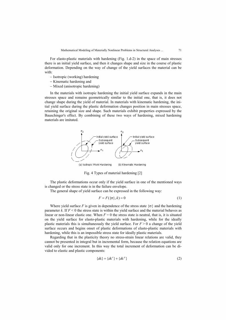
In the materials with isotropic hardening the initial yield surface expands in the main stresses space and remains geometrically similar to the initial one, that is, it does not change shape during the yield of material. In materials with kinematic hardening, the ini-tial yield surface during the plastic deformation changes position in main stresses space, retaining the original size and shape. Such materials exhibit properties expressed by the Bauschinger's effect. By combining of these two ways of hardening, mixed hardening materials are imitated.

Fig. 4 Types of material hardening [2]

The plastic deformations occur only if the yield surface in one of the mentioned ways is changed or the stress state is in the failure envelope.

The general shape of yield surface can be expressed in the following way:

0)},({ =σ= kFF (1)

Where yield surface F is given in dependence of the stress state {σ} and the hardening parameter k. If F < 0 the stress state is within the yield surface and the material behaves as linear or non-linear elastic one. When F = 0 the stress state is neutral, that is, it is situated on the yield surface for elasto-plastic materials with hardening, while for the ideally plastic materials this is simultaneously the yield surface. For F > 0 a change of the yield surface occurs and begins onset of plastic deformations of elasto-plastic materials with hardening, while this is an impossible stress state for ideally plastic materials.

Regarding that in the plasticity theory no stress-strain linear relations are valid, they cannot be presented in integral but in incremental form, because the relation equations are valid only for one increment. In this way the total increment of deformation can be di-vided to elastic and plastic components:

}{}{}{ pe ddd ε+ε=ε (2)


In isotropic material, the increment of elastic deformation is coaxial with the incre-ment of stress, and the direction and size are determined by the equation:

}{][}{ 1 σ=ε − dDd ee (3)

where [De] is the matrix of rigidity of material at elastic behavior, and {dσ} is the incre-ment of stress state. I order to establish a relation between the plastic component of de-formation and stress increment, an assumption is introduced, that the increment of plastic deformation is proportional to the stress gradient of size which is termed the plastic po-tential, so that:

}{

}{σ∂

∂λ=ε

Qd p (4)

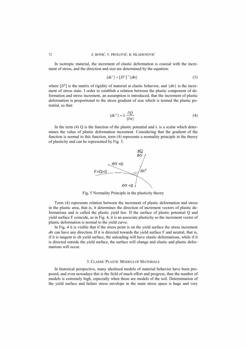
In the term (4) Q is the function of the plastic potential and λ is a scalar which deter-mines the value of plastic deformation increment. Considering that the gradient of the function is normal to this function, term (4) represents a normality principle in the theory of plasticity and can be represented by Fig. 5.

Fig. 5 Normality Principle in the plasticity theory

Term (4) represents relation between the increment of plastic deformation and stress in the plastic area, that is, it determines the direction of increment vectors of plastic de-formations and is called the plastic yield law. If the surface of plastic potential Q and yield surface F coincide, as in Fig. 4, it is an associate plasticity so the increment vector of plastic deformation is normal to the yield curve.

In Fig. 4 it is visible that if the stress point is on the yield surface the stress increment dσ can have any direction. If it is directed towards the yield surface F and neutral, that is, if it is tangent to eh yield surface, the unloading will have elastic deformations, while if it is directed outside the yield surface, the surface will change and elastic and plastic defor-mations will occur.

3. CLASSIC PLASTIC MODELS OF MATERIALS

In historical perspective, many idealized models of material behavior have been pro-posed, and even nowadays this is the field of much effort and progress, thus the number of models is extremely high, especially when those are models of the soil. Determination of the yield surface and failure stress envelope in the main stress space is huge and very


complex issue. For this reason, idealizations were introduced, so that the problem could be solved more easily and obtained solution applicable in practice. Many of the proposed models did not match the experimental results, so they are only interesting from the his-torical point of view. Here, only some of the models which were affirmed in practice will be presented.

The simple models which include the plastic properties in the description of material behavior are ideally elasto-plastic models. Working hardening or weakening is not present in them so all the yield surfaces in the spatial stress state are blended into one – final sur-face called the failure surface. Inside the failure surface, material behaves as linear-elas-tic, and when the stress state is on the yield surface a plastic deformation occurs whose di-rection and value are determined on the basis of potential function and failure conditions.

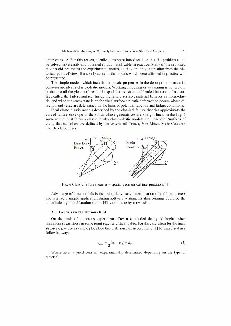
Ideal elasto-plastic models described by the classical failure theories approximate the curved failure envelope to the solids whose generatrices are straight lines. In the Fig. 6 some of the most famous classic ideally elasto-plastic models are presented. Surfaces of yield, that is, failure are defined by the criteria of: Tresca, Von Mises, Mohr-Coulomb and Drucker-Prager.

Fig. 6 Classic failure theories – spatial geometrical interpretation. [4]

Advantage of these models is their simplicity, easy determination of yield parameters and relatively simple application during software writing. Its shortcomings could be the unrealistically high dilatation and inability to imitate hysterestesis.

3.1. Tresca's yield criterion (1864)

On the basis of numerous experiments Tresca concluded that yield begins when maximum shear stress in some point reaches critical value. For the case when for the main stresses σ1, σ2, σ3 is valid σ1 ≥ σ2 ≥ σ3 this criterion can, according to [1] be expressed in a following way:

Tk=σ−σ=τ )(21

31max (5)

Where kT is a yield constant experimentally determined depending on the type of material.


The value of the constant kT can be determined from the test of uniaxial stress in de-pendence of the tensile yield stress σT. For this case of stress, σ1 = σT, a σ1 = σ2 = 0, so that the following results from the term (5):

2T

Tk σ= (6)

The value of constant kT can be determined from the pure shear test depending on the shear yield stress. In such case of stress σ1 = −σ3 = σT a σ3 = 0 so from the expression (5) it is:

TTk τ= (7)

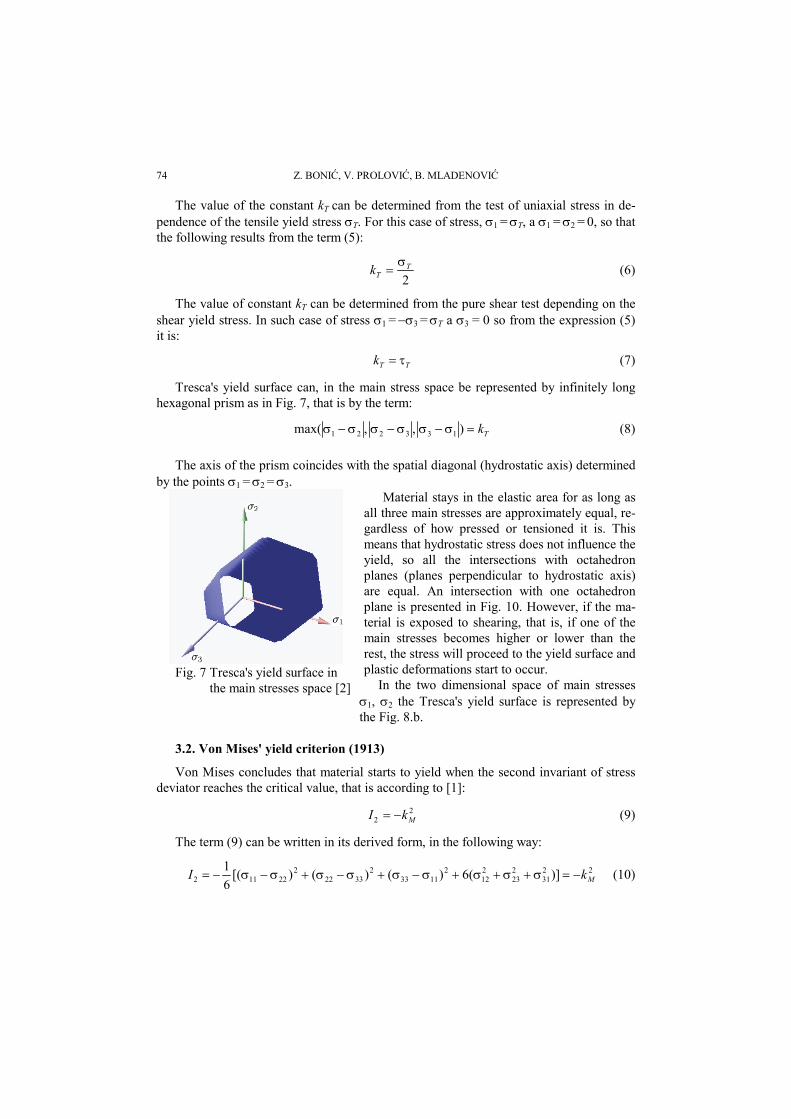
Tresca's yield surface can, in the main stress space be represented by infinitely long hexagonal prism as in Fig. 7, that is by the term:

Tk=σ−σσ−σσ−σ ),,max( 133221 (8)

The axis of the prism coincides with the spatial diagonal (hydrostatic axis) determined by the points σ1 = σ2 = σ3.

Fig. 7 Tresca's yield surface in

the main stresses space [2]

Material stays in the elastic area for as long as all three main stresses are approximately equal, re-gardless of how pressed or tensioned it is. This means that hydrostatic stress does not influence the yield, so all the intersections with octahedron planes (planes perpendicular to hydrostatic axis) are equal. An intersection with one octahedron plane is presented in Fig. 10. However, if the ma-terial is exposed to shearing, that is, if one of the main stresses becomes higher or lower than the rest, the stress will proceed to the yield surface and plastic deformations start to occur.

In the two dimensional space of main stresses σ1, σ2 the Tresca's yield surface is represented by the Fig. 8.b.

3.2. Von Mises' yield criterion (1913)

Von Mises concludes that material starts to yield when the second invariant of stress deviator reaches the critical value, that is according to [1]:

22 MkI −= (9)

The term (9) can be written in its derived form, in the following way:

2231

223

212

21133

23322

222112 )](6)()()[(

61

MkI −=σ+σ+σ+σ−σ+σ−σ+σ−σ−= (10)


The value of the yield constant kM can be determined from the test of uniaxial stress where σ11 = σT while other stress components are equal to zero. Then the term (9) is transformed into:

22

31

MT k=σ that is 3T

Mk σ= (11)

On the basis of the previous statements, the yield surface is:

3TF σ

−= (12)

For this model too, the value kM can be determined form the pure shear test where σ11 = σ22 = σ33 = σ23 = σ31 = 0, so that the result is:

TMk τ= (13)

In the three-dimensional space of main stresses σ1, σ2, σ3 von Mises' yield surface is circular cylinder whose axis, as in the Tresca's yield surface, coincides with hydrostatic axis. Intersection of both yield surfaces with the planes σ1, σ2 is presented in the Fig. 8.b.

a) b)

Fig. 8 Von Mises' yield surface in: a) three-dimensional space of the main stresses σ1, σ2, σ3 and b) in two-dimensional space of the main stresses σ1, σ2 [2]

The tests on many metals demonstrated that Von Mises' criterion is in much better ac-cordance with the results of experiments in respect to the Tresca's criterion. In spite of that, Tresca's criterion is much more frequently applied, primarily due to the simplicity of application.

3.3. Mohr-Coulomb yield criterion (1882)

The starting point here is long known Coulomb condition of soil failure (1773) which states that the failure occurs when the shear stress in a plane reaches the value:

ϕ⋅σ+=τ tgc (14)


In the term (14) c and ϕ are cohesion and angle of interior soil friction, where the adopted convention is that the pressure stress is positive.

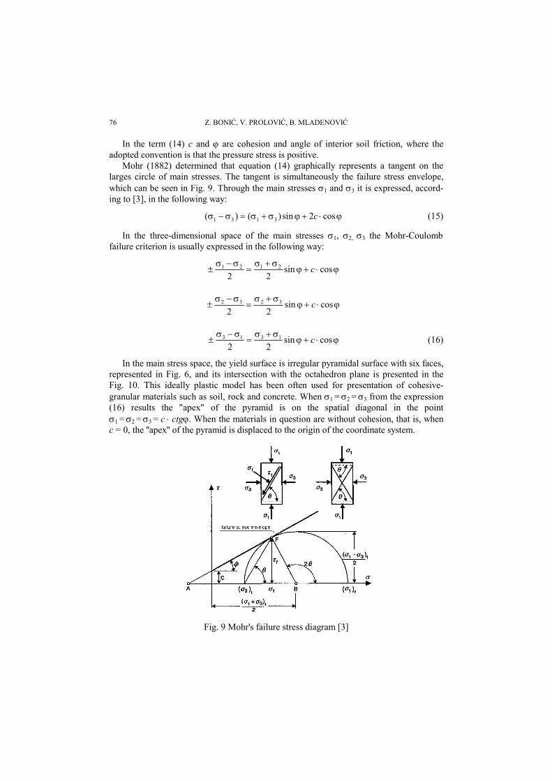
Mohr (1882) determined that equation (14) graphically represents a tangent on the larges circle of main stresses. The tangent is simultaneously the failure stress envelope, which can be seen in Fig. 9. Through the main stresses σ1 and σ3 it is expressed, accord-ing to [3], in the following way:

ϕ⋅+ϕσ+σ=σ−σ cos2sin)()( 3131 c (15)

In the three-dimensional space of the main stresses σ1, σ2, σ3 the Mohr-Coulomb failure criterion is usually expressed in the following way:

ϕ⋅+ϕσ+σ

=σ−σ

± cossin22

2121 c

ϕ⋅+ϕσ+σ

=σ−σ

± cossin22

3232 c

ϕ⋅+ϕσ+σ

=σ−σ

± cossin22

1313 c (16)

In the main stress space, the yield surface is irregular pyramidal surface with six faces, represented in Fig. 6, and its intersection with the octahedron plane is presented in the Fig. 10. This ideally plastic model has been often used for presentation of cohesive-granular materials such as soil, rock and concrete. When σ1 = σ2 = σ3 from the expression (16) results the "apex" of the pyramid is on the spatial diagonal in the point σ1 = σ2 = σ3 = c ⋅ ctgϕ. When the materials in question are without cohesion, that is, when c = 0, the ''apex'' of the pyramid is displaced to the origin of the coordinate system.

Fig. 9 Mohr's failure stress diagram [3]


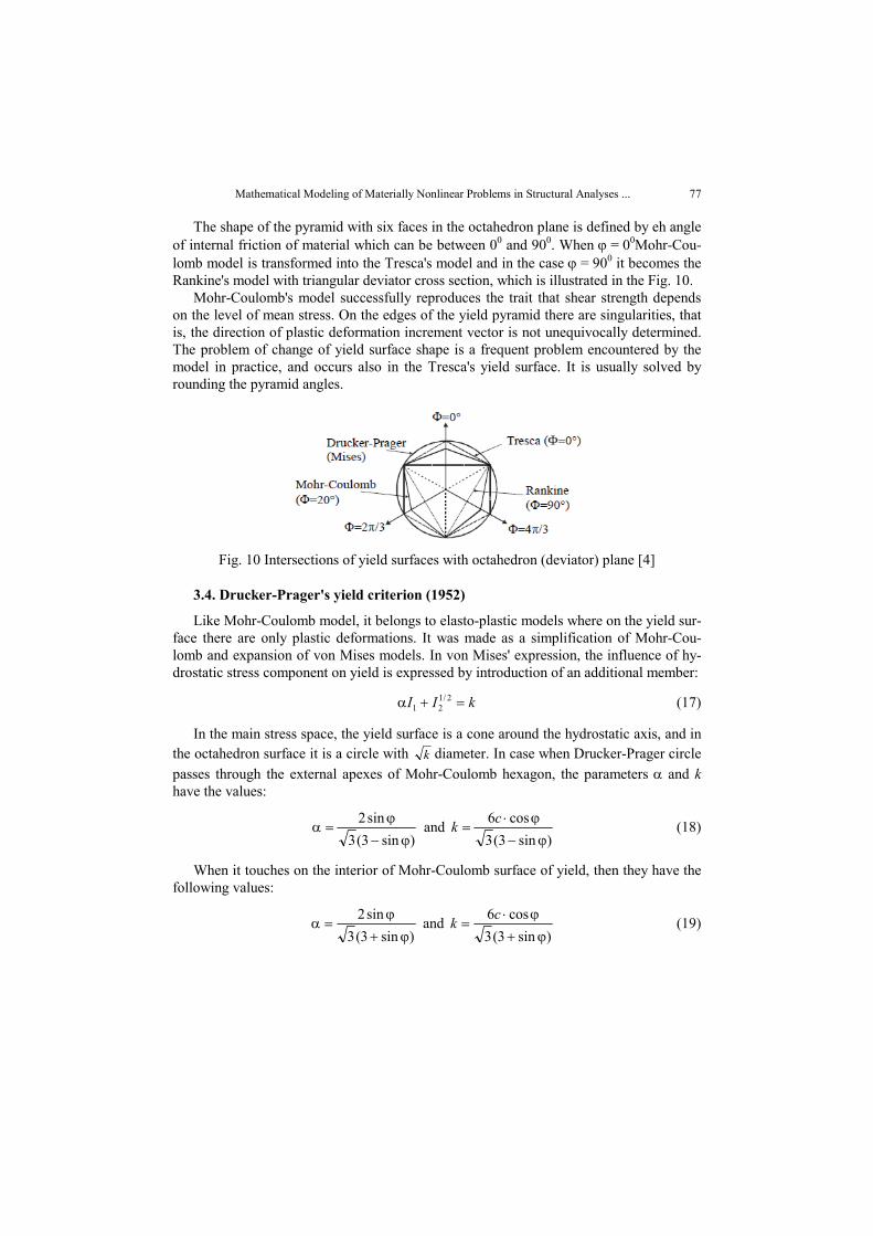
The shape of the pyramid with six faces in the octahedron plane is defined by eh angle of internal friction of material which can be between 00 and 900. When ϕ = 00Mohr-Cou-lomb model is transformed into the Tresca's model and in the case ϕ = 900 it becomes the Rankine's model with triangular deviator cross section, which is illustrated in the Fig. 10.

Mohr-Coulomb's model successfully reproduces the trait that shear strength depends on the level of mean stress. On the edges of the yield pyramid there are singularities, that is, the direction of plastic deformation increment vector is not unequivocally determined. The problem of change of yield surface shape is a frequent problem encountered by the model in practice, and occurs also in the Tresca's yield surface. It is usually solved by rounding the pyramid angles.

Fig. 10 Intersections of yield surfaces with octahedron (deviator) plane [4]

3.4. Drucker-Prager's yield criterion (1952)

Like Mohr-Coulomb model, it belongs to elasto-plastic models where on the yield sur-face there are only plastic deformations. It was made as a simplification of Mohr-Cou-lomb and expansion of von Mises models. In von Mises' expression, the influence of hy-drostatic stress component on yield is expressed by introduction of an additional member:

kII =+α 2/121 (17)

In the main stress space, the yield surface is a cone around the hydrostatic axis, and in the octahedron surface it is a circle with k diameter. In case when Drucker-Prager circle passes through the external apexes of Mohr-Coulomb hexagon, the parameters α and k have the values:

)sin3(3

sin2ϕ−

ϕ=α and

)sin3(3cos6

ϕ−ϕ⋅

=ck (18)

When it touches on the interior of Mohr-Coulomb surface of yield, then they have the following values:

)sin3(3

sin2ϕ+

ϕ=α and

)sin3(3cos6

ϕ+ϕ⋅

=ck (19)


5. CONCLUSION

Establishment of constitutive relations in order to define the way of behavior of mate-rials under external load is a complex process even in the simplest ideally elastic and ide-ally plastic models. Considering that they, nowadays cannot describe in a satisfactory way the real behavior of materials in all conditions of usage, the model theory developed in the direction of introduction of more quality elasto-plastic models into calculation. Fur-ther development is a continuous process, where new models are created and which de-scribe the nature of the materials progressively better. Apart from that the development of computer technology made possible that many of them are practically applied in calcula-tions. In the following paper, which is a continuation of this one, the models used in the Ansys software package.

REFERENCES 1. Dunica Š.: Otpornost materijala, Građevinski fakultet, Beograd 1995. 2. http://en.wikipedia.org/wiki/Yield_surface 3. Igić T.: Otpornost materijala sa elementima elastoplastičnog ponašanja konstrukcija, Građevionsko-arhi-

tektonski fakultet Niš, 2007. 4. Maksimović M.: Mehanika tla, Grosknjiga, Beograd, 1995. 5. Roje-Bonacci T.: Mehanika tla, Građevinsko-arhitektonski fakultet Sveučilišta u Splitu, 2007. 6. Santrač P.: Analiza ponašanja trakastog temelja na pesku, doktorska disertacija, Građ. fakultet, Beograd, 1999. 7. Verruijt A.: Soil Mechanics, Delft University of Technology, 2001. 8. Save M. A., Massonnet C. E., De Saxce G.: Plastic limit analysis of plates, shells and disks, Elsevier, 1997.

MATEMATIČKO MODELIRANJE MATERIJALNO NELINEARNIH PROBLEMA U ANALIZI KONSTRUKCIJA

(I DEO – TEORIJSKE OSNOVE)

Zoran Bonić, Verka Prolović, Biljana Mladenović

Modeli materijala opisuju način njihovog ponašanja pri opterećivanju. U radu je predstavljen razvoj modela počevši od najjednostavnijih linearno elastičnih i krutoplastičnih do znatno složenijih idealno elastoplastičnih. Definisani su osnovni pojmovi teorije plastičnosti kao što su kriterijum i površ tečenja (popuštanja), zakon ojačanja, zakon plastičnog tečenja i uslov normalnosti. Posebno su dati kriterijumi tečenja Tresca-e, Von Mises-a, Mohr-Coulomb-a i Drucker-Prager-a.

Ključne reči: materijalni modeli, plastičnost, kriterijum tečenja, površ tečenja

MATHEMATICAL MODELING OF MATERIALLY NONLINEAR PROBLEMS · PDF fileMATHEMATICAL MODELING OF...

Documents

Transcript of MATHEMATICAL MODELING OF MATERIALLY NONLINEAR PROBLEMS · PDF fileMATHEMATICAL MODELING OF...