
Math Programming Our Focus - York University
15
© Copyright 2003, Alan Marshall 1 Lecture 1 Lecture 1 Linear Programming © Copyright 2003, Alan Marshall 2 Agenda Agenda >Math Programming >Linear Programming • Introduction • Exercise: Lego Enterprises • Terminology, Definitions • Possible Outcomes • Sensitivity Analysis © Copyright 2003, Alan Marshall 3 Math Programming Math Programming >Deals with resource allocation to maximize or minimize an objective subject to certain constraints >Types: • Linear, Integer, Mixed, Nonlinear, Goal >Relatively easy to solve using modern computing technology (potentially too easy!) © Copyright 2003, Alan Marshall 4 Our Focus Our Focus >Linear, Integer (& Mixed Linear/Integer) >Recognizing when linear/integer/mixed programming is appropriate >Developing basic models >Computer solution • Excel >Interpreting results © Copyright 2003, Alan Marshall 5 Lego Enterprises Lego Enterprises >Table profit is $16; Chair profit is $10 >Table design • 2 large blocks (side by side) • 2 small blocks (stacked under, centered) >Chair design • 1 large block (seat) • 2 small blocks (back, bottom) >Objective: select product mix to maximize profits using available resources © Copyright 2003, Alan Marshall 6 Understanding Lego Problem Understanding Lego Problem > Formulate as LP • Decision Variables, Objective Function, Constraints >Graph • Constraints, Objective function >Find solution
Transcript of Math Programming Our Focus - York University

© Copyright 2003, Alan Marshall 1
Lecture 1Lecture 1
Linear Programming
© Copyright 2003, Alan Marshall 2
AgendaAgenda
>Math Programming>Linear Programming
• Introduction• Exercise: Lego Enterprises• Terminology, Definitions• Possible Outcomes• Sensitivity Analysis
© Copyright 2003, Alan Marshall 3
Math ProgrammingMath Programming
>Deals with resource allocation tomaximize or minimize an objectivesubject to certain constraints
>Types:• Linear, Integer, Mixed, Nonlinear, Goal
>Relatively easy to solve using moderncomputing technology (potentially tooeasy!)
© Copyright 2003, Alan Marshall 4
Our FocusOur Focus
>Linear, Integer (& MixedLinear/Integer)
>Recognizing whenlinear/integer/mixed programming isappropriate
>Developing basic models>Computer solution
• Excel
>Interpreting results
© Copyright 2003, Alan Marshall 5
Lego EnterprisesLego Enterprises
>Table profit is $16; Chair profit is $10>Table design
• 2 large blocks (side by side)• 2 small blocks (stacked under, centered)
>Chair design• 1 large block (seat)• 2 small blocks (back, bottom)
>Objective: select product mix tomaximize profits using availableresources
© Copyright 2003, Alan Marshall 6
Understanding Lego ProblemUnderstanding Lego Problem
> Formulate as LP• Decision Variables, Objective Function,
Constraints
>Graph• Constraints, Objective function
>Find solution

© Copyright 2003, Alan Marshall 7
LP FormulationLP Formulation
>Decision Variables• T = # of tables• C = # of chairs
>Objective• Maximize profit =
>Constraints• For large blocks:• For small blocks:
© Copyright 2003, Alan Marshall 8
LP FormulationLP Formulation
>Decision Variables• T = # of tables• C = # of chairs
>Objective• Maximize profit: Z = 16T + 10C
>Constraints• For large blocks:• For small blocks:
© Copyright 2003, Alan Marshall 9
LP FormulationLP Formulation
>Decision Variables• T = # of tables• C = # of chairs
>Objective• Maximize profit: Z = 16T + 10C
>Constraints• For large blocks: 2T + 1C < 6• For small blocks:
© Copyright 2003, Alan Marshall 10
LP FormulationLP Formulation
>Decision Variables• T = # of tables• C = # of chairs
>Objective• Maximize profit: Z = 16T + 10C
>Constraints• For large blocks: 2T + 1C < 6• For small blocks: 2T + 2C < 8
© Copyright 2003, Alan Marshall 11
Graphing Lego ExampleGraphing Lego Example
>Draw quadrant & axes• use T on x-axis and C on y-axis
>Add constraint lines• Find intercepts: set T to zero and solve
for C, set C to zero and solve for T
>Add profit equation• Select reasonable value
>Move profit equation outwards, as faras feasible
© Copyright 2003, Alan Marshall 12
Graphing Lego ExampleGraphing Lego Example
>Draw quadrant &axes• use T on x-axis and
C on y-axis
Lego Problem
0
1
2
3
4
5
6
7
8
0 1 2 3 4 5Tables
Chai
rs

© Copyright 2003, Alan Marshall 13
Graphing Lego ExampleGraphing Lego Example
>Add constraint lines• Find intercepts: set
T to zero and solvefor C, set C to zeroand solve for T
>Large:• Tables: Max = 3• Chairs: Max = 6
Lego Problem
0
1
2
3
4
5
6
7
8
0 1 2 3 4 5
Tables
Chai
rs
© Copyright 2003, Alan Marshall 14
Graphing Lego ExampleGraphing Lego Example
>Add constraint lines• Find intercepts: set
T to zero and solvefor C, set C to zeroand solve for T
>Large:• Tables: Max = 3• Chairs: Max = 6
Lego Problem
0
1
2
3
4
5
6
7
8
0 1 2 3 4 5
Tables
Chai
rs
© Copyright 2003, Alan Marshall 15
Graphing Lego ExampleGraphing Lego Example
>Add constraint lines• Find intercepts: set
T to zero and solvefor C, set C to zeroand solve for T
>Small:• Tables: Max = 4• Chairs: Max = 4
Lego Problem
0
1
2
3
4
5
6
7
8
0 1 2 3 4 5
Tables
Chai
rs
© Copyright 2003, Alan Marshall 16
Graphing Lego ExampleGraphing Lego Example
>Add constraint lines• Find intercepts: set
T to zero and solvefor C, set C to zeroand solve for T
>Small:• Tables: Max = 4• Chairs: Max = 4
Lego Problem
0
1
2
3
4
5
6
7
8
0 1 2 3 4 5
Tables
Chai
rs
© Copyright 2003, Alan Marshall 17
Graphing Lego ExampleGraphing Lego Example
>Add profit equation• Select reasonable
value
>40:• Tables: 40/16 = 2.5• Chairs: 40/10 = 4
Lego Problem
0
1
2
3
4
5
6
7
8
0 1 2 3 4 5
Tables
Chai
rs
© Copyright 2003, Alan Marshall 18
Graphing Lego ExampleGraphing Lego Example
>Add profit equation• Select reasonable
value
>40:• Tables: 40/16 = 2.5• Chairs: 40/10 = 4
Lego Problem
0
1
2
3
4
5
6
7
8
0 1 2 3 4 5
Tables
Chai
rs

© Copyright 2003, Alan Marshall 19
Graphing Lego ExampleGraphing Lego Example
>Move profitequation outwards,as far as feasible
>Solution: T = 2, C= 2
>Profit:16(2)+10(2)=52
Lego Problem
0
1
2
3
4
5
6
7
8
0 1 2 3 4 5
Tables
Chai
rs
© Copyright 2003, Alan Marshall 20
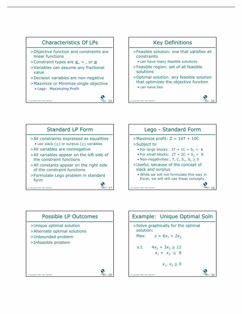
Characteristics Of LPsCharacteristics Of LPs
>Objective function and constraints arelinear functions
>Constraint types are <, = , or >>Variables can assume any fractional
value>Decision variables are non-negative>Maximize or Minimize single objective
© Copyright 2003, Alan Marshall 21
Characteristics Of LPsCharacteristics Of LPs
>Objective function and constraints arelinear functions• Lego: All were linear trade-offs
>Constraint types are <, = , or >>Variables can assume any fractional
value>Decision variables are non-negative>Maximize or Minimize single objective
© Copyright 2003, Alan Marshall 22
Characteristics Of LPsCharacteristics Of LPs
>Objective function and constraints arelinear functions
>Constraint types are <, = , or >• Lego: All Constraints implied maximums
(<)
>Variables can assume any fractionalvalue
>Decision variables are non-negative>Maximize or Minimize single objective
© Copyright 2003, Alan Marshall 23
Characteristics Of LPsCharacteristics Of LPs
>Objective function and constraints arelinear functions
>Constraint types are <, = , or >>Variables can assume any fractional
value• Lego: Fractional values can be viewed as
work-in-process at the end of the day
>Decision variables are non-negative>Maximize or Minimize single objective
© Copyright 2003, Alan Marshall 24
Characteristics Of LPsCharacteristics Of LPs
>Objective function and constraints arelinear functions
>Constraint types are <, = , or >>Variables can assume any fractional
value>Decision variables are non-negative
• Lego: Cannot produce negative amounts
>Maximize or Minimize single objective
© Copyright 2003, Alan Marshall 25
Characteristics Of LPsCharacteristics Of LPs
>Objective function and constraints arelinear functions
>Constraint types are <, = , or >>Variables can assume any fractional
value>Decision variables are non-negative>Maximize or Minimize single objective
• Lego: Maximizing Profit
© Copyright 2003, Alan Marshall 26
Key DefinitionsKey Definitions
>Feasible solution: one that satisfies allconstraints• can have many feasible solutions
>Feasible region: set of all feasiblesolutions
>Optimal solution: any feasible solutionthat optimizes the objective function• can have ties
© Copyright 2003, Alan Marshall 27
Standard LP FormStandard LP Form
>All constraints expressed as equalities• use slack (<) or surplus (>) variables
>All variables are nonnegative>All variables appear on the left side of
the constraint functions>All constants appear on the right side
of the constraint functions>Formulate Lego problem in standard
form
© Copyright 2003, Alan Marshall 28
Lego - Standard FormLego - Standard Form
>Maximize profit: Z = 16T + 10C>Subject to
• For large blocks: 2T + 1C + S1 = 6• For small blocks: 2T + 2C + S2 = 8• Non-negativities:, T, C, S1, S2 > 0
>Useful, because of the concept ofslack and surplus• While we will not formulate this way in
Excel, we will still use these concepts
© Copyright 2003, Alan Marshall 29
Possible LP OutcomesPossible LP Outcomes
>Unique optimal solution>Alternate optimal solutions>Unbounded problem>Infeasible problem
© Copyright 2003, Alan Marshall 30
Example: Unique Optimal SolnExample: Unique Optimal Soln
>Solve graphically for the optimalsolution:Max: z = 6x1 + 2x2
s.t. 4x1 + 3x2 > 12x1 + x2 < 8
x1, x2 > 0
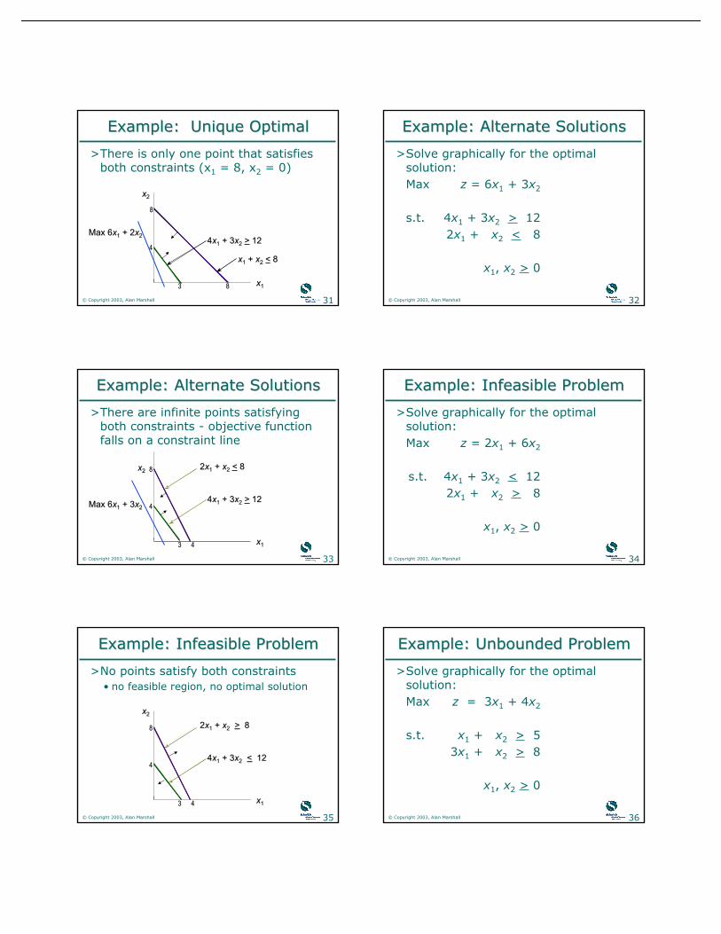
© Copyright 2003, Alan Marshall 31
xx22
xx11
44xx11 + 3 + 3xx22 >> 12 12
xx11 + + xx22 << 8 8
33 88
44
88
Max 6Max 6xx11 + 2 + 2xx22
Example: Unique OptimalExample: Unique Optimal
>There is only one point that satisfiesboth constraints (x1 = 8, x2 = 0)
© Copyright 2003, Alan Marshall 32
Example: Alternate SolutionsExample: Alternate Solutions
>Solve graphically for the optimalsolution:Max z = 6x1 + 3x2
s.t. 4x1 + 3x2 > 122x1 + x2 < 8
x1, x2 > 0
© Copyright 2003, Alan Marshall 33
xx22
xx11
44xx11 + 3 + 3xx22 >> 12 12
22xx11 + + xx22 << 8 8
33 44
44
88
Max 6Max 6xx11 + 3 + 3xx22
Example: Alternate SolutionsExample: Alternate Solutions
>There are infinite points satisfyingboth constraints - objective functionfalls on a constraint line
© Copyright 2003, Alan Marshall 34
Example: Infeasible ProblemExample: Infeasible Problem
>Solve graphically for the optimalsolution:Max z = 2x1 + 6x2
s.t. 4x1 + 3x2 < 122x1 + x2 > 8
x1, x2 > 0
© Copyright 2003, Alan Marshall 35
xx22
xx11
44xx11 + 3 + 3xx22 << 12 12
22xx11 + + xx22 >> 8 8
33 44
44
88
Example: Infeasible ProblemExample: Infeasible Problem
>No points satisfy both constraints• no feasible region, no optimal solution
© Copyright 2003, Alan Marshall 36
Example: Unbounded ProblemExample: Unbounded Problem
>Solve graphically for the optimalsolution:Max z = 3x1 + 4x2
s.t. x1 + x2 > 53x1 + x2 > 8
x1, x2 > 0

© Copyright 2003, Alan Marshall 37
x2
x1
33xx11 + + xx22 >> 8 8
xx11 + + xx22 >> 5 5
Max 3Max 3xx11 + 4 + 4xx22
5
5
88
2.67
Example: Unbounded ProblemExample: Unbounded Problem
>objective function can be movedoutward without limit; z can beincreased infinitely
© Copyright 2003, Alan Marshall 38
RECAPRECAP
© Copyright 2003, Alan Marshall 39
Characteristics Of LPsCharacteristics Of LPs
>Objective function and constraints arelinear functions
>Constraint types are <, = , or >>Variables can assume any fractional
value>Decision variables are non-negative>Maximize or Minimize single objective
© Copyright 2003, Alan Marshall 40
FormulationFormulation
>Define decision variables: x1, x2, …>Objective Function (max, min)>s.t., with constraints listed
• Variables on left side• Constants on right side• All variables nonnegative
>NB: “Standard Form” requiresconstraints stated as equalities• add slack/surplus variables
© Copyright 2003, Alan Marshall 41
Possible LP OutcomesPossible LP Outcomes
>Unique optimal solution>Alternate optimal solutions>Unbounded problem>Infeasible problem
© Copyright 2003, Alan Marshall 42
BreakBreak
15 Minutes

© Copyright 2003, Alan Marshall 43
LP Models: Key QuestionsLP Models: Key Questions
>What am I trying to decide?>What is the objective?
• Is it to be minimized or maximized?
>What are the constraints?• Are they limitations or requirements?• Are they explicit or implicit?
© Copyright 2003, Alan Marshall 44
ExampleExample
A chemical company makes and sells a productin 40-lb. and 80-lb. bags on a commonproduction line. To meet anticipated orders,next week’s production should be at least16,000 lbs. Profit contributions are $2 per 40-lb. bag, and $4 per 80-lb. bag. The packagingline operates 1500 minutes/week. 40-lb. bagsrequire 1.2 min. of packaging time; 80-lb.bags require 3 min. The company has 6000square feet of packaging material available.Each 40-lb. bag uses 6 square feet, and each80-lb. bag uses 10 square feet. How manybags of each type should be produced?
© Copyright 2003, Alan Marshall 45
Model DevelopmentModel Development
>What do we need to decide?What are our decision variables?
© Copyright 2003, Alan Marshall 46
Model DevelopmentModel Development
>What do we need to decide?x1 = number of 40-lb. bags to producex2 = number of 80-lb. bags to produce
© Copyright 2003, Alan Marshall 47
Model DevelopmentModel Development
>What is the objective?
© Copyright 2003, Alan Marshall 48
Model DevelopmentModel Development
>What is the objective?Maximize total profit

© Copyright 2003, Alan Marshall 49
Model DevelopmentModel Development
>What is the objective?Maximize total profitz = 2x1 + 4x2
© Copyright 2003, Alan Marshall 50
Check Your Units!Check Your Units!
>Always be sure that your units areconsistent with the problem
>Our decision variable is measured in “Bags”>Our profit/objective function is in $
$bagsbag$
tObj.Fn.UniitDec.Var.Unf.Obj.Fn.Coe
=×
=×
© Copyright 2003, Alan Marshall 51
Model DevelopmentModel Development
>What are the constraints?
© Copyright 2003, Alan Marshall 52
Model DevelopmentModel Development
>What are the constraints?Aggregate production:Packaging time:Packaging materials:Nonnegativity:
© Copyright 2003, Alan Marshall 53
Model DevelopmentModel Development
>What are the constraints?Prod: 40x1 + 80x2 > 16,000Time:Mat:NN:
© Copyright 2003, Alan Marshall 54
Model DevelopmentModel Development
>What are the constraints?Prod: 40x1 + 80x2 > 16,000Time: 1.2x1 + 3x2 < 1,500Mat:NN:

© Copyright 2003, Alan Marshall 55
Model DevelopmentModel Development
>What are the constraints?Prod: 40x1 + 80x2 > 16,000Time: 1.2x1 + 3x2 < 1,500Mat: 6x1 + 10x2 < 6,000NN:
© Copyright 2003, Alan Marshall 56
Model DevelopmentModel Development
>What are the constraints?Prod: 40x1 + 80x2 > 16,000Time: 1.2x1 + 3x2 < 1,500Mat: 6x1 + 10x2 < 6,000NN: x1, x2 > 0
© Copyright 2003, Alan Marshall 57
Check The Units!Check The Units!
>What are the constraints?Prod: 40x1 + 80x2 > 16,000 lbs/bag x bagsTime: 1.2x1 + 3x2 < 1,500 min/bag x bagsMat: 6x1 + 10x2 < 6,000 ft2/bag x bagsNN: x1, x2 > 0
© Copyright 2003, Alan Marshall 58
Complete ModelComplete Model
x1 = no. of 40-lb. bags to producex2 = no. of 80-lb. bags to produceMaximize z = 2x1 + 4x2
subject to 40x1 + 80x2 > 16,000 1.2x1 + 3x2 < 1,500 6x1 + 10x2 < 6,000 x1, x2 > 0
© Copyright 2003, Alan Marshall 59
ExcelExcel
>Model Input• Basic model• Solver: identify objective function &
constraints
>Results• Answer Report• Sensitivity Report• Limits Report
© Copyright 2003, Alan Marshall 60
Spreadsheet ModelSpreadsheet Model
A B C D E F G1 40-lb 80-lb23 DecVar 0 04 Constraint Constraint5 ObFnCoef 2 4 0 Amount Slack67 MinProd'n 40 80 0 >= 16000 160008 MachTime 1.2 3 0 <= 1500 15009 PackMat 6 10 0 <= 6000 6000

© Copyright 2003, Alan Marshall 61
Cell FormulasCell Formulas
A B C D E F G1 40-lb 80-lb23 DecVar 0 04 Constraint Constraint5 ObFnCoef 2 4 =SUMPRODUCT(B5:C5,$B$3:$C$3) Amount Slack67 MinProd'n 40 80 =SUMPRODUCT(B7:C7,$B$3:$C$3) >= 16000 =ROUND(F7-D7,2)8 MachTime 1.2 3 =SUMPRODUCT(B8:C8,$B$3:$C$3) <= 1500 =ROUND(F8-D8,2)9 PackMat 6 10 =SUMPRODUCT(B9:C9,$B$3:$C$3) <= 6000 =ROUND(F9-D9,2)
© Copyright 2003, Alan Marshall 62
Using SolverUsing Solver
© Copyright 2003, Alan Marshall 63
Adding ConstraintsAdding Constraints
© Copyright 2003, Alan Marshall 64
Note Assumptionsticked - essential!
Solver OptionsSolver Options
© Copyright 2003, Alan Marshall 65
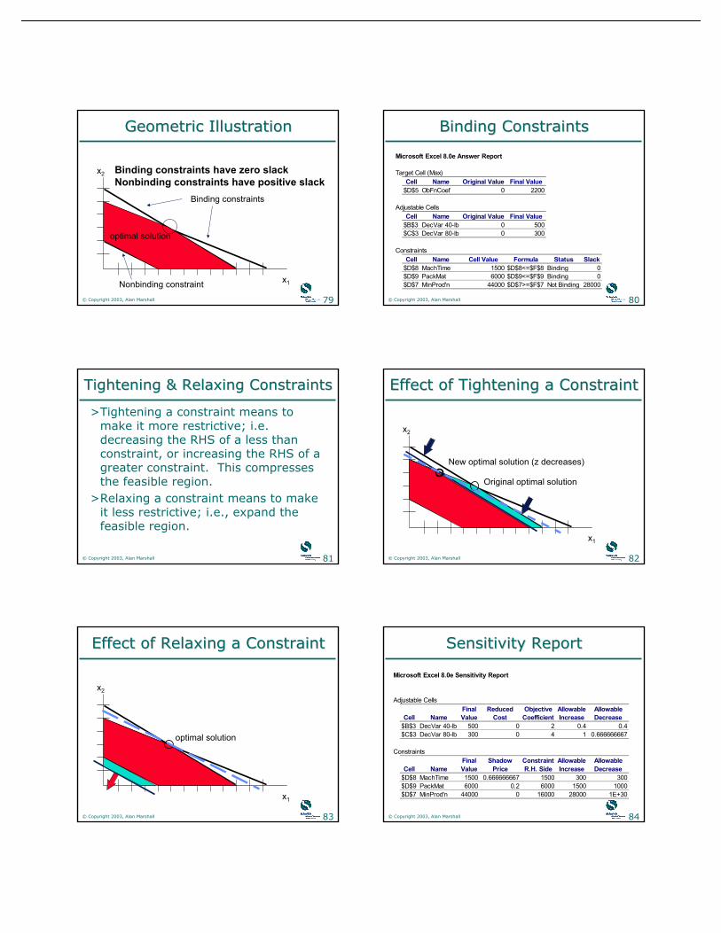
Answer ReportAnswer Report
Microsoft Excel 8.0e Answer Report
Target Cell (Max)Cell Name Original Value Final Value
$D$5 ObFnCoef 0 2200
Adjustable CellsCell Name Original Value Final Value
$B$3 DecVar 40-lb 0 500$C$3 DecVar 80-lb 0 300
ConstraintsCell Name Cell Value Formula Status Slack
$D$8 MachTime 1500 $D$8<=$F$8 Binding 0$D$9 PackMat 6000 $D$9<=$F$9 Binding 0$D$7 MinProd'n 44000 $D$7>=$F$7 Not Binding 28000
© Copyright 2003, Alan Marshall 66
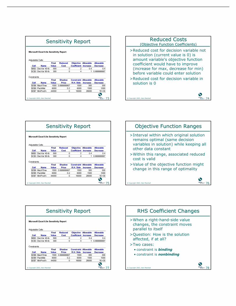
Sensitivity ReportSensitivity Report
Microsoft Excel 8.0e Sensitivity Report
Adjustable CellsFinal Reduced Objective Allowable Allowable
Cell Name Value Cost Coefficient Increase Decrease$B$3 DecVar 40-lb 500 0 2 0.4 0.4$C$3 DecVar 80-lb 300 0 4 1 0.666666667
ConstraintsFinal Shadow Constraint Allowable Allowable
Cell Name Value Price R.H. Side Increase Decrease$D$8 MachTime 1500 0.666666667 1500 300 300$D$9 PackMat 6000 0.2 6000 1500 1000$D$7 MinProd'n 44000 0 16000 28000 1E+30

© Copyright 2003, Alan Marshall 67
Optimal SolutionOptimal Solution
>Three parts:• decision variables• values of decision variables• value of objective function
>Decision variables:• basic (non-zero value),• non-basic (zero)• Basic variables are “in the solution”; non-
basic are not
© Copyright 2003, Alan Marshall 68
Impact of Possible ChangesImpact of Possible Changes
>Change existing constraint• changes slope; may change size of
feasible region
>Add new constraint• may decrease feasible region (if binding)
>Remove constraint• may increase feasible region (if binding)
>Change objective• may change optimal solution
© Copyright 2003, Alan Marshall 69
Sensitivity AnalysisSensitivity Analysis
>The next section will deal with thesensitivity analysis that can be donesimply based on the reports generated,without rerunning the solution.
>While this can be useful, mastery of thismaterial is not important for the course,or programme as you can always simplyrun the model again with the changes
>However, we will look at this briefly
© Copyright 2003, Alan Marshall 70
Sensitivity AnalysisSensitivity Analysis
>Used to determine how optimalsolution is affected by changes, withinspecified ranges: objective function orRHS coefficients (only 1 at a time)
>Important to managers who mustoperate in a dynamic environmentwith imprecise estimates ofcoefficients
>Sensitivity analysis allows us to askcertain what-if questions
© Copyright 2003, Alan Marshall 71
Objective Function CoefficientsObjective Function Coefficients
>If an objective function coefficientchanges, slope of objective functionline changes. At some threshold,another corner point may becomeoptimal.
>Question: How much can objectivecoefficient change without changingoptimal corner point?
© Copyright 2003, Alan Marshall 72
x2
x1
current optimal solution
new optimal solution
Geometric IllustrationGeometric Illustration
© Copyright 2003, Alan Marshall 73
Sensitivity ReportSensitivity Report
Microsoft Excel 8.0e Sensitivity Report
Adjustable CellsFinal Reduced Objective Allowable Allowable
Cell Name Value Cost Coefficient Increase Decrease$B$3 DecVar 40-lb 500 0 2 0.4 0.4$C$3 DecVar 80-lb 300 0 4 1 0.666666667
ConstraintsFinal Shadow Constraint Allowable Allowable
Cell Name Value Price R.H. Side Increase Decrease$D$8 MachTime 1500 0.666666667 1500 300 300$D$9 PackMat 6000 0.2 6000 1500 1000$D$7 MinProd'n 44000 0 16000 28000 1E+30
© Copyright 2003, Alan Marshall 74
Reduced CostsReduced Costs(Objective Function Coefficients)(Objective Function Coefficients)
>Reduced cost for decision variable notin solution (current value is 0) isamount variable's objective functioncoefficient would have to improve(increase for max, decrease for min)before variable could enter solution
>Reduced cost for decision variable insolution is 0
© Copyright 2003, Alan Marshall 75
Sensitivity ReportSensitivity Report
Microsoft Excel 8.0e Sensitivity Report
Adjustable CellsFinal Reduced Objective Allowable Allowable
Cell Name Value Cost Coefficient Increase Decrease$B$3 DecVar 40-lb 500 0 2 0.4 0.4$C$3 DecVar 80-lb 300 0 4 1 0.666666667
ConstraintsFinal Shadow Constraint Allowable Allowable
Cell Name Value Price R.H. Side Increase Decrease$D$8 MachTime 1500 0.666666667 1500 300 300$D$9 PackMat 6000 0.2 6000 1500 1000$D$7 MinProd'n 44000 0 16000 28000 1E+30
© Copyright 2003, Alan Marshall 76
Objective Function RangesObjective Function Ranges
>Interval within which original solutionremains optimal (same decisionvariables in solution) while keeping allother data constant
>Within this range, associated reducedcost is valid
>Value of the objective function mightchange in this range of optimality
© Copyright 2003, Alan Marshall 77
Sensitivity ReportSensitivity Report
Microsoft Excel 8.0e Sensitivity Report
Adjustable CellsFinal Reduced Objective Allowable Allowable
Cell Name Value Cost Coefficient Increase Decrease$B$3 DecVar 40-lb 500 0 2 0.4 0.4$C$3 DecVar 80-lb 300 0 4 1 0.666666667
ConstraintsFinal Shadow Constraint Allowable Allowable
Cell Name Value Price R.H. Side Increase Decrease$D$8 MachTime 1500 0.666666667 1500 300 300$D$9 PackMat 6000 0.2 6000 1500 1000$D$7 MinProd'n 44000 0 16000 28000 1E+30
© Copyright 2003, Alan Marshall 78
RHS Coefficient ChangesRHS Coefficient Changes
>When a right-hand-side valuechanges, the constraint movesparallel to itself
>Question: How is the solutionaffected, if at all?
>Two cases:• constraint is binding• constraint is nonbinding
© Copyright 2003, Alan Marshall 79
x2
x1
optimal solution
Binding constraints
Binding constraints have zero slackNonbinding constraints have positive slack
Nonbinding constraint
Geometric IllustrationGeometric Illustration
© Copyright 2003, Alan Marshall 80
Binding ConstraintsBinding Constraints
Microsoft Excel 8.0e Answer Report
Target Cell (Max)Cell Name Original Value Final Value
$D$5 ObFnCoef 0 2200
Adjustable CellsCell Name Original Value Final Value
$B$3 DecVar 40-lb 0 500$C$3 DecVar 80-lb 0 300
ConstraintsCell Name Cell Value Formula Status Slack
$D$8 MachTime 1500 $D$8<=$F$8 Binding 0$D$9 PackMat 6000 $D$9<=$F$9 Binding 0$D$7 MinProd'n 44000 $D$7>=$F$7 Not Binding 28000
© Copyright 2003, Alan Marshall 81
Tightening & Relaxing ConstraintsTightening & Relaxing Constraints
>Tightening a constraint means tomake it more restrictive; i.e.decreasing the RHS of a less thanconstraint, or increasing the RHS of agreater constraint. This compressesthe feasible region.
>Relaxing a constraint means to makeit less restrictive; i.e., expand thefeasible region.
© Copyright 2003, Alan Marshall 82
x2
x1
Original optimal solution
New optimal solution (z decreases)
Effect of Tightening a ConstraintEffect of Tightening a Constraint
© Copyright 2003, Alan Marshall 83
x2
x1
optimal solution
Effect of Relaxing a ConstraintEffect of Relaxing a Constraint
© Copyright 2003, Alan Marshall 84
Sensitivity ReportSensitivity Report
Microsoft Excel 8.0e Sensitivity Report
Adjustable CellsFinal Reduced Objective Allowable Allowable
Cell Name Value Cost Coefficient Increase Decrease$B$3 DecVar 40-lb 500 0 2 0.4 0.4$C$3 DecVar 80-lb 300 0 4 1 0.666666667
ConstraintsFinal Shadow Constraint Allowable Allowable
Cell Name Value Price R.H. Side Increase Decrease$D$8 MachTime 1500 0.666666667 1500 300 300$D$9 PackMat 6000 0.2 6000 1500 1000$D$7 MinProd'n 44000 0 16000 28000 1E+30

© Copyright 2003, Alan Marshall 85
Dual Prices (RHS Coefficients)Dual Prices (RHS Coefficients)
>Amount objective function will improveper unit increase in constraint RHS value
>Reflects value of an additional unit ofresource (if resource cost is sunk);reflects extra value over normal cost ofresource (when resource cost isrelevant)
>Always 0 for nonbinding constraint(positive slack or surplus at optimalsolution)
© Copyright 2003, Alan Marshall 86
Sensitivity ReportSensitivity Report
Microsoft Excel 8.0e Sensitivity Report
Adjustable CellsFinal Reduced Objective Allowable Allowable
Cell Name Value Cost Coefficient Increase Decrease$B$3 DecVar 40-lb 500 0 2 0.4 0.4$C$3 DecVar 80-lb 300 0 4 1 0.666666667
ConstraintsFinal Shadow Constraint Allowable Allowable
Cell Name Value Price R.H. Side Increase Decrease$D$8 MachTime 1500 0.666666667 1500 300 300$D$9 PackMat 6000 0.2 6000 1500 1000$D$7 MinProd'n 44000 0 16000 28000 1E+30
© Copyright 2003, Alan Marshall 87
Sensitivity ReportSensitivity Report
Microsoft Excel 8.0e Sensitivity Report
Adjustable CellsFinal Reduced Objective Allowable Allowable
Cell Name Value Cost Coefficient Increase Decrease$B$3 DecVar 40-lb 500 0 2 0.4 0.4$C$3 DecVar 80-lb 300 0 4 1 0.666666667
ConstraintsFinal Shadow Constraint Allowable Allowable
Cell Name Value Price R.H. Side Increase Decrease$D$8 MachTime 1500 0.666666667 1500 300 300$D$9 PackMat 6000 0.2 6000 1500 1000$D$7 MinProd'n 44000 0 16000 28000 1E+30
© Copyright 2003, Alan Marshall 88
RHS RangesRHS Ranges
>As long as the constraint RHScoefficient stays within this range, theassociated dual price is valid
>For changes outside this range, mustresolve
© Copyright 2003, Alan Marshall 89
Shadow vs Dual PricesShadow vs Dual Prices
>Shadow Price: Amount objectivefunction will change per unit increasein RHS value of constraint
>For maximization problems, dualprices and shadow prices are thesame
>For minimization problems, shadowprices are the negative of dual prices
© Copyright 2003, Alan Marshall 90
Next ClassNext Class
>We will look at the two handoutexercises• To be posted on the website, with
solution files
>Decision Theory>In Lecture 3, we will do additional
problems in both Linear Programmingand Decision Theory


![Singapore Math Scope & Sequence [Math in Focus]](https://static.fdocuments.us/doc/165x107/5517cbbe497959a8308b4cd0/singapore-math-scope-sequence-math-in-focus.jpg)