MATH 131A: REAL ANALYSIS
48
MATH 131A: REAL ANALYSIS NICKOLAS ANDERSEN The textbook for the course is Ross, Elementary Analysis [2], but in these notes I have also borrowed from Tao, Analysis I [3], and Abbott, Understanding Analysis [1]. 1. Introduction Real analysis is a rigorous study of the (hopefully familiar) objects from calculus: the real numbers, functions, limits, continuity, derivatives, sequences, series, and integrals. While you are likely quite familiar with computing with these objects, this course will focus on developing the theoretical foundation for the definitions, theorems, formulas, and algorithms that you are used to using. We will start by building up the real numbers from scratch, i.e., from just a few basic axioms, then we will focus our attention on proving many of the things you already believe about functions, sequences, and series. Along the way we will encounter several “pathological” objects which will hopefully convince you that our careful approch is necessary and worthwhile. To get an idea of how subtle some questions in analysis can be, ask yourself: what is a real number? We will answer this question in due time, but for now let’s focus on one specific real number that got a lot of attention from the ancient Greeks: √ 2. Prior to the discovery that √ 2 is an irrational number, it was assumed that: given any two line segments AB and CD, there is a rational number r so that the length of CD equals r times the length of AB. However, the length of the diagonal of a square of side length 1 (using the Pythagorean Theorem) equals √ 2, so by the previous assumption, we must have that √ 2 is a rational number. The proof of the following theorem is one of the most classic proofs in mathematics. Theorem 1.1. There is no rational number whose square is 2. Proof. Suppose that x 2 = 2 and that x is a rational number. Recall that a rational number is one which can be expressed as p/q for integers p and q. To prove that there are no integers p, q for which x = p/q we will employ an important proof technique called proof by contradiction. That is, we will assume that x = p/q for some integers p, q and we will carefully follow logical steps until we end up with something absurd. Thus, our original assumption must have been faulty. Here we go. Suppose that there are integers p, q for which p q 2 =2. (1.1) We may assume that p and q have no common factors, since we could just cancel the common factors and write p/q in lowest terms. Equation (1.1) implies that p 2 =2q 2 . (1.2) It follows that p 2 is an even number (it’s 2 times an integer), and therefore p is an even number (you can’t square an odd number and get an even number). So we can write p =2r 1
Transcript of MATH 131A: REAL ANALYSIS
MATH 131A: REAL ANALYSIS
NICKOLAS ANDERSEN
The textbook for the course is Ross, Elementary Analysis [2], but in these notes I havealso borrowed from Tao, Analysis I [3], and Abbott, Understanding Analysis [1].
1. Introduction
Real analysis is a rigorous study of the (hopefully familiar) objects from calculus: the realnumbers, functions, limits, continuity, derivatives, sequences, series, and integrals. Whileyou are likely quite familiar with computing with these objects, this course will focus ondeveloping the theoretical foundation for the definitions, theorems, formulas, and algorithmsthat you are used to using. We will start by building up the real numbers from scratch, i.e.,from just a few basic axioms, then we will focus our attention on proving many of the thingsyou already believe about functions, sequences, and series. Along the way we will encounterseveral “pathological” objects which will hopefully convince you that our careful approch isnecessary and worthwhile.
To get an idea of how subtle some questions in analysis can be, ask yourself: what is a realnumber? We will answer this question in due time, but for now let’s focus on one specificreal number that got a lot of attention from the ancient Greeks:
√2. Prior to the discovery
that√
2 is an irrational number, it was assumed that: given any two line segments AB andCD, there is a rational number r so that the length of CD equals r times the length ofAB. However, the length of the diagonal of a square of side length 1 (using the PythagoreanTheorem) equals
√2, so by the previous assumption, we must have that
√2 is a rational
number. The proof of the following theorem is one of the most classic proofs in mathematics.
Theorem 1.1. There is no rational number whose square is 2.
Proof. Suppose that x2 = 2 and that x is a rational number. Recall that a rational numberis one which can be expressed as p/q for integers p and q. To prove that there are nointegers p, q for which x = p/q we will employ an important proof technique called proofby contradiction. That is, we will assume that x = p/q for some integers p, q and we willcarefully follow logical steps until we end up with something absurd. Thus, our originalassumption must have been faulty. Here we go.
Suppose that there are integers p, q for which(p
q
)2
= 2. (1.1)
We may assume that p and q have no common factors, since we could just cancel the commonfactors and write p/q in lowest terms. Equation (1.1) implies that
p2 = 2q2. (1.2)
It follows that p2 is an even number (it’s 2 times an integer), and therefore p is an evennumber (you can’t square an odd number and get an even number). So we can write p = 2r
1
2 NICKOLAS ANDERSEN
for some integer r. Then equation (1.2) becomes (after cancelling 2s)
2r2 = q2.
By the previous discussion, this implies that q is even. But that’s ridiculous! We assumedthat p and q had no factors in common, but we just showed that p and q were both even.Since we have reached a contradiction, it must be that our inital assumption (1.1) was false.Thus 2 is not the square of any rational number. �
The previous theorem shows that there is a “hole” at√
2 in the rational numbers. Theimportance of this fact cannot be overstated. Later it will lead us to the Axiom of Com-pleteness which is an essential property that the real numbers enjoy which basically statesthat there are no holes in the set of real numbers. This will lead us to limits, derivatives,continuity, and eventually integrals. But first we need to take a few steps back and start atthe beginning.
2. The natural numbers
If our aim is to construct the real numbers and do calculus on the set of real numbers,then we must start with the simplest numbers first and build our way up. Thus our storybegins with the natural numbers (a.k.a whole numbers or counting numbers) which we caninformally define as the elements of the set
N := {1, 2, 3, 4, 5, . . .}.We are no longer in the business of informal definitions, so we’ll need to build N from scratch.In excruciating detail.
Let’s think about what we want in a set of numbers. In mathematics, it is often desirablenot to think too carefully about the actual elements in a set, but more about what youwant those elements to do (i.e. what operations or functions do you want to apply to thoseelements?). A few moments of thought might lead you to say that the most important thingwe do with the natural numbers is counting (you might have said addition or multiplication,but addition is just repeated counting, and multiplication is just repeated addition). So itstands to reason that we should construct the natural numbers so that we can count withthem.
We will begin with two concepts: the number 1, and the successor n + 1. Note that wehaven’t defined addition yet (we don’t even know what the numbers are!) so n + 1 doesn’tmean n “plus” 1. Yet. It’s just an expression that we use to denote the successor of n.Informally (but less informally than before), we will define the natural numbers as the setcontaining 1, the successor 1 + 1, the successor (1 + 1) + 1, the successor ((1 + 1) + 1) + 1,etc. This leads to our first two axioms.
Axiom 1: 1 is a natural number.
Axiom 2: If n is a natural number, then n+ 1 is a natural number.
By Axioms 1 and 2, we see that
((((((1 + 1) + 1) + 1) + 1) + 1) + 1) + 1
is a natural number. Don’t worry, we won’t write numbers like this; instead we’ll use thenotation we’re all familiar with. So the number above is called 8. But for now, the symbol8 means nothing other than a shorthand notation for the successor of the successor of thesuccessor of the successor of the successor of the successor of the successor of 1.
MATH 131A: REAL ANALYSIS 3
It may seem like this is enough to define the natural numbers, but consider the set con-sisting of all natural numbers from 1 to 12, where the successor of 12 is 1 (this is not somecrazy thing, it’s how clocks work!). Even though this number system obeys Axioms 1 and2, it doesn’t even allow us to count how many fingers and toes we have, so it must not beright. Let’s add another axiom.
Axiom 3: 1 is not the successor of any natural number; i.e. n+ 1 6= 1 for all n.
Now we can prove statements like the following.
Lemma 2.1. 4 6= 1.
Proof. By definition 4 = 3 + 1. By Axioms 1 and 2, 3 is a natural number (since 3 =(1 + 1) + 1). Thus by Axiom 3, 3 + 1 6= 1. Therefore 4 6= 1. �
At this rate we’ll never get to derivatives! (Don’t worry, we’re going to go through theconstruction of the natural numbers in painful detail so that you can see what goes into arigorous mathematical foundation of analysis. Then we will move a bit faster so that we cancover other things.)
Have we constructed N yet? Unfortunately, there are still weird pathological numbersystems which satisfy the first three axioms, but which are not the natural numbers (as wewould like them to be). Consider the number system
1, 1 + 1 = 2, 2 + 1 = 3, 3 + 1 = 4, 4 + 1 = 4, 4 + 1 = 4, . . . .
You can check that this doesn’t break our first three axioms, but it’s still definitely not right.Let’s add another axiom.
Axiom 4: If n and m are natural numbers and n 6= m then n+ 1 6= m+ 1.
Equivalently, if n+ 1 = m+ 1 then n = m.
Now we can’t have the above pathology.
Lemma 2.2. 4 6= 2.
Proof. Suppose, by way of contradiction, that 4 = 2. Then 3 + 1 = 1 + 1, so by Axiom 4we have 3 = 1. But that contradicts Axiom 3, so our original assumption must have beenwrong. Thus 4 6= 2. �
We’re not out of the woods yet. We have constructed a set of axioms which confirms thatall of the numbers that we think should be natural numbers (i.e. 1, 2, 3, . . .) are elements ofN. But we can’t rule out the existence of other numbers masquerading as natural numbers.For example, the set
{.5, 1, 1.5, 2, 2.5, 3, 3.5, 4, . . .}satisfies all of the axioms so far. So we’ll need one final axiom. This one is so importantthat it gets its own name. (You’ll want to chew on this one for a bit.)
Axiom 5 (The principle of mathematical induction):
Let Pn be any statement or proposition that may or may not be true.
Suppose that P1 is true, and that whenever Pn is true, Pn+1 is also true.
Then Pn is true for every natural number n.
The principle of mathematical induction allows us to prove that a statement is true bysimply checking two things: first we check that the statement is true for n = 1, then,
4 NICKOLAS ANDERSEN
assuming it is true for n, we check that it is true for n + 1. Here is an example (note: thisexample really belongs later in the course, after we’ve defined addition and multiplicationand division, but I’m happy to time travel for a few seconds if you are).
Proposition 2.3. For all natural numbers n we have
1 + 2 + . . .+ n =n(n+ 1)
2.
Proof. For each n, the statement we want to prove is
Pn : “1 + 2 + . . .+ n =n(n+ 1)
2.”
We proceed by induction. We begin with P1, which states that 1 = 1(1+1)2
. This is certainlytrue. Suppose that Pn is true, i.e. suppose that
1 + 2 + . . .+ n =n(n+ 1)
2is a true statement. We wish to show that Pn+1 is true. Add n+ 1 to both sides to obtain
1 + 2 + . . .+ n+ n+ 1 =n(n+ 1)
2+ n+ 1
=(n+ 1)(n+ 1 + 1)
2.
Thus Pn+1 holds if Pn holds. By the principle of mathematical induction, Pn holds for allnatural numbers n. �
Note that we didn’t prove Pn directly for any n except for n = 1. We just proved P1, andwe proved that if P1 is true, so is P2 (thus P2 is true), and we proved that if P2 is true, so isP3 (thus P3 is true), and we proved that if P3 is true, so is P4 (thus P4 is true), etc. It’s likestacking up an infinite line of dominoes and knocking over the first one.
Since we will use induction regularly to prove things in lecture, homework, and exams, itmight be useful to have a template for such proofs.
Proposition 2.4. A property Pn is true for all natural numbers n.
Proof. We proceed by induction on n (it’s good to specify the variable if there are severalvariables in the statement you want to prove). We first verify the base case n = 1, i.e. weprove that P1 is true. [Insert proof of P1 here]. Now suppose that Pn has already beenproven. We show that Pn+1 is true. [Insert proof of Pn+1, assuming Pn]. It follows that Pnis true for all natural numbers n. �
3. The integers and the rationals
At this point, if we had all the time in the world, we would maintain the glacial paceof the last section and carefully develop the theory of addition and multiplication on thenatural numbers. But for the sake of time (and to maintain our sanity) we will take somethings for granted as we build up the integers and the rational numbers. This means that thediscussion in the section will be quite informal. I hope our careful approach to the naturalnumbers was enough to convince you that there is a careful way to construct the integersand the rational numbers from the natural numbers. If you would like to learn about this inmore detail, see [3].
MATH 131A: REAL ANALYSIS 5
Informally, the set of integers is made up of the positive integers, the negative integersand 0. We know the positive integers well; these are just the natural numbers. We can add(2 + 3 = 5) and multiply (2 · 3 = 6) natural numbers as usual. (Formally, m+n is defined asapplying the successor to m, n times; multiplication is then defined as repeated addition.)These operations satisfy the rules
a+ b = b+ a, (commutative law for addition)
(a+ b) + c = a+ (b+ c), (associative law for addition)
a · b = b · a, (commutative law for multiplication)
(a · b) · c = a · (b · c), (associative law for multiplication)
a · 1 = a, (multiplicative identity)
(a+ b) · c = a · c+ b · c. (distributive law)
In order to define subtraction, we introduce the additive inverse of a number and theadditive identity element. The additive identity element, 0, is defined by its behavior underaddition via
n+ 0 = 0 + n = n. (additive identity)
(Note: we could have defined the natural numbers to include 0, and some authors do this.But Ross [2] doesn’t, so we won’t.) For each natural number n, the additive inverse of n,which we will call −n, is defined by the property
n+ (−n) = (−n) + n = 0. (additive inverse)
Subtraction is then defined via
a− b := a+ (−b).(Note: here I’m being quite informal and sweeping some subtleties under the rug. Forexample, we would like to say that the integers 1 − 5 and 2 − 6 and 3 − 7, etc., are allthe same, but the definition I’ve given you above doesn’t account for that. But to do thisproperly, we would have to introduce the notion of equivalence classes, which we won’t dohere. See Tao’s book [3] if you are interested in learning more.)
We define the integers as the elements of the set
Z := N ∪ {0} ∪ (−N).
Here −N is the set consisting of the additive inverses of all the natural numbers, i.e., thenegative integers. The notation ∪ means union. For any two sets A and B, the set A ∪ Bconsists of all the elements that are in A and/or B. As you are already aware, the laws listedabove extend to the entire set Z of integers. Using these laws, we can prove some familiarproperties of integers.
Proposition 3.1. Suppose that a, b, c ∈ Z. Then
(1) a+ c = b+ c implies that a = b,(2) a · 0 = 0,(3) (−a) · b = −(a · b),(4) (−a) · (−b) = a · b,(5) a · b = 0 implies that a = 0 or b = 0 (or both),(6) a · c = b · c and c 6= 0 together imply that a = b.
6 NICKOLAS ANDERSEN
Proof. (1) If a + c = b + c then (a + c) + (−c) = (b + c) + (−c). So by associativityof addition we have a + (c + (−c)) = b + (c + (−c)). Then by the additive inverseproperty, we have a + 0 = b + 0, and by the additive identity property, we concludethat a = b.
(2) By the additive identity property and the distributive law we have
0 + a · 0 = a · 0 = a · (0 + 0) = a · 0 + a · 0.
Using (1) we find that 0 = a · 0.(3) Starting with a+ (−a) = 0, we multiply both sides by b and use the distributive law
to see that
a · b+ (−a) · b = (a+ (−a)) · b = 0 · b = 0,
where we have used (2) in the last equality. Thus we see that (−a) · b = −(a · b).(4) Exercise.(5) We will prove that a, b 6= 0 implies that a · b 6= 0 (convince yourself that this is
enough! This is an example of proof using contrapositive).First assume that a, b ∈ N. Then since multiplication is repeated addition, which is
the same as taking the successor repeatedly, by Axiom 3 we cannot have a·b = 0 (thisis slightly informal, but since we never formally defined addition or multiplication,I’m going to let it slide).
Now suppose that a ∈ (−N) and b ∈ N. Then a = −n for some n ∈ N, and by(3) we have a · b = (−n) · b = −(n · b). Since n, b ∈ N, the previous case shows thatn · b 6= 0, so −(n · b) 6= 0.
Now suppose that a, b ∈ (−N). Then a = −m and b = −n for some m,n ∈ N, andby (4) we have a · b = (−m) · (−n) = m · n. Since m,n ∈ N, the first case appliesagain and we have m · n 6= 0.
(6) Exercise. �
Just as we defined subtraction by creating the negative integers and using addition, we candefine division by creating reciprocals and using multiplication. For each nonzero integer n,we define the multiplicative inverse n−1 by the relation
n · n−1 = n−1 · n = 1. (multiplicative inverse)
Division is then defined by (assuming that b 6= 0)
a/b := a · b−1,
and the rational numbers are all of the numbers a/b for a, b ∈ Z with b 6= 0. We use Q todenote the set of rational numbers. In set-builder notation,
Q :={ab
: a, b ∈ Z and b 6= 0}.
(As with subtraction, we have some subtelty here: we would like to think of the rationalnumbers 1/2 and 2/4 and 3/6 as being equal. To do this properly requires an equivalencerelation; see [3] for more details if you are interested.)
As you know already, the rational numbers Q inherit the same properties as the integers,along with the properties listed in Proposition 3.1. For completeness, we list them all together
MATH 131A: REAL ANALYSIS 7
here. If a, b, c ∈ Q then
a+ b = b+ a, (commutative law for addition)
(a+ b) + c = a+ (b+ c), (associative law for addition)
n+ 0 = n, (additive identity)
n+ (−n) = 0, (additive inverse)
a · b = b · a, (commutative law for multiplication)
(a · b) · c = a · (b · c), (associative law for multiplication)
a · 1 = a, (multiplicative identity)
n · n−1 = 1, (multiplicative inverse)
(a+ b) · c = a · c+ b · c. (distributive law)
A number system which satisfies all of these properties (and for which 0 6= 1; that would beweird) is called a field.
The set field Q is actually an ordered field, which means that it has an order structure ≤which obeys the following rules (which you are already familiar with):
(O1) For all a, b ∈ Q, either a ≤ b or b ≤ a.(O2) If a ≤ b and b ≤ a then a = b.(O3) If a ≤ b and b ≤ c then a ≤ c.(O4) If a ≤ b then a+ c ≤ b+ c.(O5) If a ≤ b and c ≥ 0 then ac ≤ bc.
Using these rules, we can prove the following properties. Note that a > b means that a ≥ band a 6= b.
Proposition 3.2. If a, b, c ∈ Q then the following properties hold.
(1) If a ≤ b then −a ≥ −b.(2) If a ≤ b and c ≤ 0 then ac ≥ bc.(3) If a ≥ 0 and b ≥ 0 then ab ≥ 0.(4) a2 ≥ 0 for all a.(5) 0 < 1.(6) If a > 0 then a−1 > 0.(7) If 0 < a < b then 0 < b−1 < a−1.
Proof. (1) We apply (O4) with c = (−a) + (−b). If a ≤ b then
−b = −b+ a+ (−a) = a+ (−a) + (−b) ≤ b+ (−a) + (−b) = (−a) + b+ (−b) = −a,
as desired.(2) Suppose that c ≤ 0. Then by (1) we have −c ≥ 0. If a ≤ b then by (O5) we have
(−c)a ≤ (−c)b which implies that −(ac) ≤ −(bc). Applying (1) again we find thatac ≥ bc.
(3) Follows immediately from (O5) with a = 0.(4) By (O1), either a ≥ 0 or a ≤ 0. If a ≥ 0 then we apply (3) with b = a. If a ≤ 0 then
by (1) we have −a ≥ 0. By (3) again we have (−a)(−a) ≥ 0, i.e. a2 ≥ 0.(5) Exercise.
8 NICKOLAS ANDERSEN
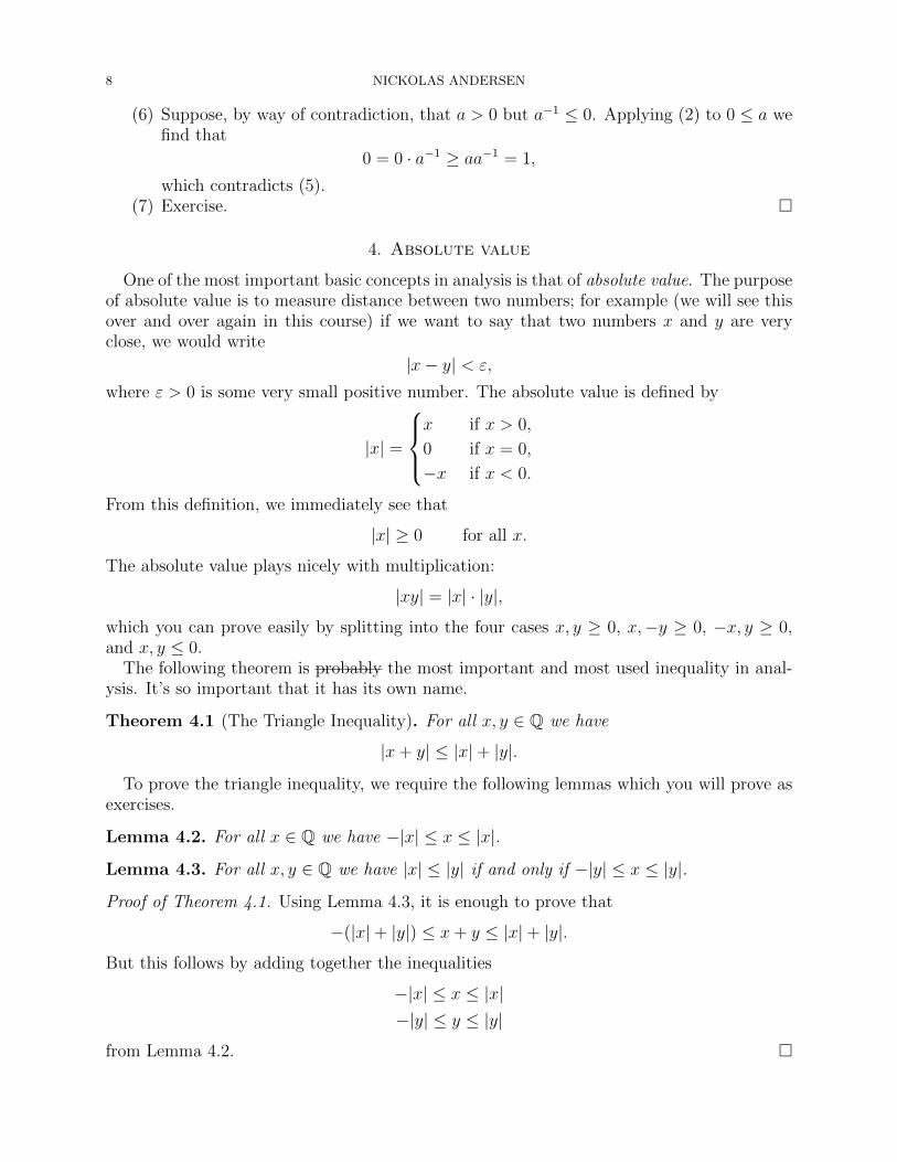
(6) Suppose, by way of contradiction, that a > 0 but a−1 ≤ 0. Applying (2) to 0 ≤ a wefind that
0 = 0 · a−1 ≥ aa−1 = 1,
which contradicts (5).(7) Exercise. �
4. Absolute value
One of the most important basic concepts in analysis is that of absolute value. The purposeof absolute value is to measure distance between two numbers; for example (we will see thisover and over again in this course) if we want to say that two numbers x and y are veryclose, we would write
|x− y| < ε,
where ε > 0 is some very small positive number. The absolute value is defined by
|x| =
x if x > 0,
0 if x = 0,
−x if x < 0.
From this definition, we immediately see that
|x| ≥ 0 for all x.
The absolute value plays nicely with multiplication:
|xy| = |x| · |y|,
which you can prove easily by splitting into the four cases x, y ≥ 0, x,−y ≥ 0, −x, y ≥ 0,and x, y ≤ 0.
The following theorem is probably the most important and most used inequality in anal-ysis. It’s so important that it has its own name.
Theorem 4.1 (The Triangle Inequality). For all x, y ∈ Q we have
|x+ y| ≤ |x|+ |y|.
To prove the triangle inequality, we require the following lemmas which you will prove asexercises.
Lemma 4.2. For all x ∈ Q we have −|x| ≤ x ≤ |x|.
Lemma 4.3. For all x, y ∈ Q we have |x| ≤ |y| if and only if −|y| ≤ x ≤ |y|.
Proof of Theorem 4.1. Using Lemma 4.3, it is enough to prove that
−(|x|+ |y|) ≤ x+ y ≤ |x|+ |y|.
But this follows by adding together the inequalities
−|x| ≤ x ≤ |x|−|y| ≤ y ≤ |y|
from Lemma 4.2. �
MATH 131A: REAL ANALYSIS 9
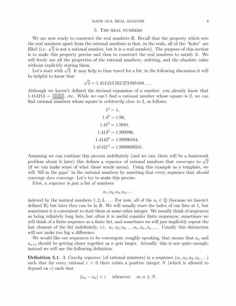
5. The real numbers
We are now ready to construct the real numbers R. Recall that the property which setsthe real numbers apart from the rational numbers is that, in the reals, all of the “holes” arefilled (i.e.
√2 is not a rational number, but it is a real number). The purpose of this section
is to make this property precise and then to construct the real numbers to satisfy it. Wewill freely use all the properties of the rational numbers, ordering, and the absolute valuewithout explicitly stating them.
Let’s start with√
2. It may help to time travel for a bit; in the following discussion it willbe helpful to know that √
2 = 1.414 213 562 373 095 048 . . . .
Although we haven’t defined the decimal expansion of a number, you already know that1.414213 = 1414213
1000000, etc. While we can’t find a rational number whose square is 2, we can
find rational numbers whose square is arbitrarily close to 2, as follows:
12 = 1,
1.42 = 1.96,
1.412 = 1.9881,
1.4142 = 1.999396,
1.41422 = 1.99996164,
1.414212 = 1.9999899241.
Assuming we can continue this process indefinitely (and we can; there will be a homeworkproblem about it later) this defines a sequence of rational numbers that converges to
√2
(if we can make sense of what those words mean). Using this example as a template, wewill “fill in the gaps” in the rational numbers by asserting that every sequence that shouldconverge does converge. Let’s try to make this precise.
First, a sequence is just a list of numbers
a1, a2, a3, a4, . . .
indexed by the natural numbers 1, 2, 3, . . .. For now, all of the ai ∈ Q (because we haven’tdefined R) but later they can be in R. We will usually start the index of our lists at 1, butsometimes it is convenient to start them at some other integer. We usually think of sequencesas being infinitely long lists, but often it is useful consider finite sequences; sometimes wewill think of a finite sequence as a finite list, and sometimes we will just implicitly repeat thelast element of the list indefinitely, i.e. a1, a2, a3, . . . an, an, an . . .. Usually this distinctionwill not make too big a difference.
We would like our sequences to be convergent; roughly speaking, that means that an andan+1 should be getting closer together as n gets larger. Actually, this is not quite enough;instead we will use the following definition.
Definition 5.1. A Cauchy sequence (of rational numbers) is a sequence (a1, a2, a3, a4, . . .)such that for every rational ε > 0 there exists a positive integer N (which is allowed todepend on ε) such that
|am − an| < ε whenever m,n ≥ N.
10 NICKOLAS ANDERSEN
Note: the restriction that ε needs to be a rational number is there purely because we don’tknow what a real number is yet. Later we will consider Cauchy sequences of real numbersand we will think of ε as being any positive real number. You should not think about thisdistinction too much, as it will not be important in the long run.
We should unpack Definition 5.1; it’s quite important to understand this well. It’s sayingthat a Cauchy sequence is a sequence whose terms eventually (i.e. there exists a positiveinteger N) get really close together (i.e. |am − an| < ε). Note that this needs to hold for allm,n ≥ N , not just n and n + 1, say. You should think of ε as being a microscopically tinynumber; so for ε = 1
10or 1
100or 1
1010or 1
10100, etc. the terms of our sequence are eventually at
most a distance of ε apart.
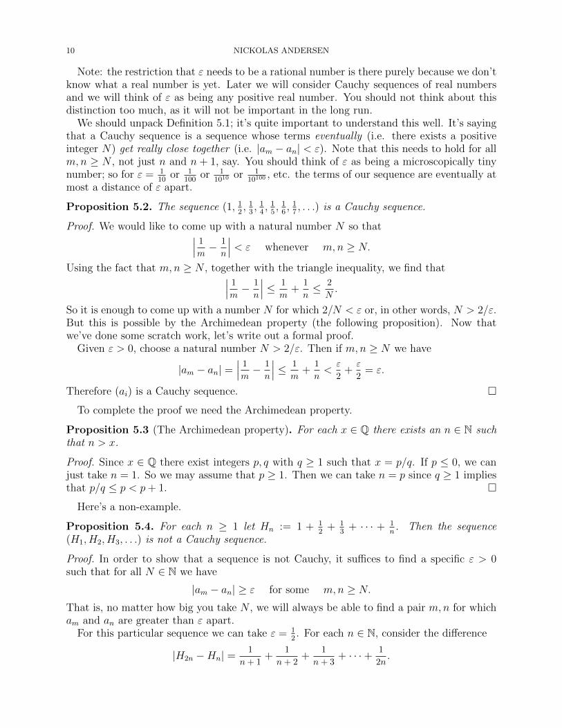
Proposition 5.2. The sequence (1, 12, 13, 14, 15, 16, 17, . . .) is a Cauchy sequence.
Proof. We would like to come up with a natural number N so that∣∣∣ 1
m− 1
n
∣∣∣ < ε whenever m,n ≥ N.
Using the fact that m,n ≥ N , together with the triangle inequality, we find that∣∣∣ 1
m− 1
n
∣∣∣ ≤ 1
m+
1
n≤ 2
N.
So it is enough to come up with a number N for which 2/N < ε or, in other words, N > 2/ε.But this is possible by the Archimedean property (the following proposition). Now thatwe’ve done some scratch work, let’s write out a formal proof.
Given ε > 0, choose a natural number N > 2/ε. Then if m,n ≥ N we have
|am − an| =∣∣∣ 1
m− 1
n
∣∣∣ ≤ 1
m+
1
n<
ε
2+
ε
2= ε.
Therefore (ai) is a Cauchy sequence. �
To complete the proof we need the Archimedean property.
Proposition 5.3 (The Archimedean property). For each x ∈ Q there exists an n ∈ N suchthat n > x.
Proof. Since x ∈ Q there exist integers p, q with q ≥ 1 such that x = p/q. If p ≤ 0, we canjust take n = 1. So we may assume that p ≥ 1. Then we can take n = p since q ≥ 1 impliesthat p/q ≤ p < p+ 1. �
Here’s a non-example.
Proposition 5.4. For each n ≥ 1 let Hn := 1 + 12
+ 13
+ · · · + 1n
. Then the sequence(H1, H2, H3, . . .) is not a Cauchy sequence.
Proof. In order to show that a sequence is not Cauchy, it suffices to find a specific ε > 0such that for all N ∈ N we have
|am − an| ≥ ε for some m,n ≥ N.
That is, no matter how big you take N , we will always be able to find a pair m,n for whicham and an are greater than ε apart.
For this particular sequence we can take ε = 12. For each n ∈ N, consider the difference
|H2n −Hn| =1
n+ 1+
1
n+ 2+
1
n+ 3+ · · ·+ 1
2n.
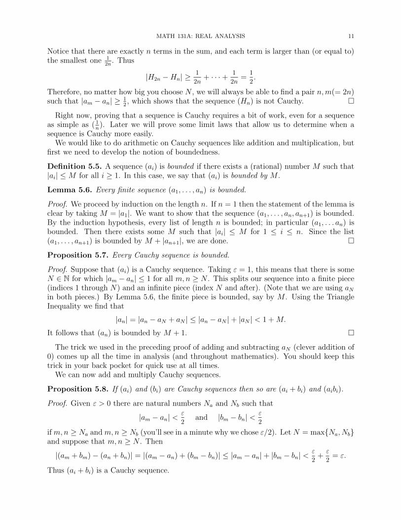
MATH 131A: REAL ANALYSIS 11
Notice that there are exactly n terms in the sum, and each term is larger than (or equal to)the smallest one 1
2n. Thus
|H2n −Hn| ≥1
2n+ · · ·+ 1
2n=
1
2.
Therefore, no matter how big you choose N , we will always be able to find a pair n,m(= 2n)such that |am − an| ≥ 1
2, which shows that the sequence (Hn) is not Cauchy. �
Right now, proving that a sequence is Cauchy requires a bit of work, even for a sequenceas simple as ( 1
n). Later we will prove some limit laws that allow us to determine when a
sequence is Cauchy more easily.We would like to do arithmetic on Cauchy sequences like addition and multiplication, but
first we need to develop the notion of boundedness.
Definition 5.5. A sequence (ai) is bounded if there exists a (rational) number M such that|ai| ≤M for all i ≥ 1. In this case, we say that (ai) is bounded by M .
Lemma 5.6. Every finite sequence (a1, . . . , an) is bounded.
Proof. We proceed by induction on the length n. If n = 1 then the statement of the lemma isclear by taking M = |a1|. We want to show that the sequence (a1, . . . , an, an+1) is bounded.By the induction hypothesis, every list of length n is bounded; in particular (a1, . . . an) isbounded. Then there exists some M such that |ai| ≤ M for 1 ≤ i ≤ n. Since the list(a1, . . . , an+1) is bounded by M + |an+1|, we are done. �
Proposition 5.7. Every Cauchy sequence is bounded.
Proof. Suppose that (ai) is a Cauchy sequence. Taking ε = 1, this means that there is someN ∈ N for which |am − an| ≤ 1 for all m,n ≥ N . This splits our sequence into a finite piece(indices 1 through N) and an infinite piece (index N and after). (Note that we are using aNin both pieces.) By Lemma 5.6, the finite piece is bounded, say by M . Using the TriangleInequality we find that
|an| = |an − aN + aN | ≤ |an − aN |+ |aN | < 1 +M.
It follows that (an) is bounded by M + 1. �
The trick we used in the preceding proof of adding and subtracting aN (clever addition of0) comes up all the time in analysis (and throughout mathematics). You should keep thistrick in your back pocket for quick use at all times.
We can now add and multiply Cauchy sequences.
Proposition 5.8. If (ai) and (bi) are Cauchy sequences then so are (ai + bi) and (aibi).
Proof. Given ε > 0 there are natural numbers Na and Nb such that
|am − an| <ε
2and |bm − bn| <
ε
2
if m,n ≥ Na and m,n ≥ Nb (you’ll see in a minute why we chose ε/2). Let N = max{Na, Nb}and suppose that m,n ≥ N . Then
|(am + bm)− (an + bn)| = |(am − an) + (bm − bn)| ≤ |am − an|+ |bm − bn| <ε
2+
ε
2= ε.
Thus (ai + bi) is a Cauchy sequence.

12 NICKOLAS ANDERSEN
For the product, use Proposition 5.7 to find Ma and Mb such that |ai| ≤Ma and |bi| ≤Mb,and set M = max{Ma,Mb}. Since (ai) and (bi) are Cauchy, there are natural numbers Na
and Nb (likely different than before) such that
|am − an| <ε
2Mand |bm − bn| <
ε
2M
if m,n ≥ Na and m,n ≥ Nb. Let N = max{Na, Nb}. Then if m,n ≥ N we have (cleverlyadding 0 again)
|ambm − anbn| = |ambm − ambn + ambn − anbn|≤ |am||bm − bn|+ |bn||am − an| < M
ε
2M+M
ε
2M< ε.
Thus (aibi) is Cauchy. �
It should be clear that since the rational numbers satisfy the commutative ring axioms(associativity and commutativity of addition and multiplication, the distributive law, etc.),so do Cauchy sequences. Is there an additive identity element? Sure, take (0, 0, 0, . . .). Whatabout a multiplicative identity element? Yes, use (1, 1, 1, . . .).
What about division? It is tempting to define division of Cauchy sequences by (an/bn)but this only works if bn 6= 0 for all n. Fine, but we don’t want to divide by the zeroelement (0, 0, 0, . . .) anyway. However, there is a catch: the sequences (1, 1, 1, 1, 1 . . .) and(1, 0, 1, 1, 1, 1, . . .) are both Cauchy sequences and they seem to have the same “limit,” namely1. So we should be able to divide by either of them; but we can’t divide by the second onein the usual way because of that pesky 0.
A more interesting example comes from the two Cauchy sequences
1, 1.4, 1.41, 1.414, 1.4142, 1.41421, . . . ,
2, 1.5, 1.42, 1.415, 1.4143, 1.41422, . . . .
Both “look like” they are converging to√
2. But none of the terms in the first sequenceare equal to their counterpart in the second sequence, so the sequnces are definitely not thesame. Our aim is eventually to define the real numbers as limits of Cauchy sequences ofrational numbers, so we should consider the two sequences above to be “the same.”
Definition 5.9. Two sequences (ai) and (bi) are equivalent if for each ε > 0 there exists anatural number N (which can depend on ε) such that
|an − bn| < ε whenever n ≥ N.
The following two propositions will allow us to define division.
Proposition 5.10. Suppose that (ai) is a Cauchy sequence that is not equivalent to the zerosequence (0, 0, 0, . . .). Then there exists a Cauchy sequence (bi) and a number m > 0, with|bi| ≥ m for all i, such that (ai) and (bi) are equivalent.
Proof. Since (ai) is not equivalent to the zero sequence, there exists a fixed number ε0 forwhich the definition of equivalent sequences fails. This means that for each N ≥ 1 thereexists a number n ≥ N for which
|an − 0| ≥ ε0.
Now, (ai) is a Cauchy sequence, so there exists some (fixed) N0 for which
|am − an| <ε02
whenever m,n ≥ N0.
MATH 131A: REAL ANALYSIS 13
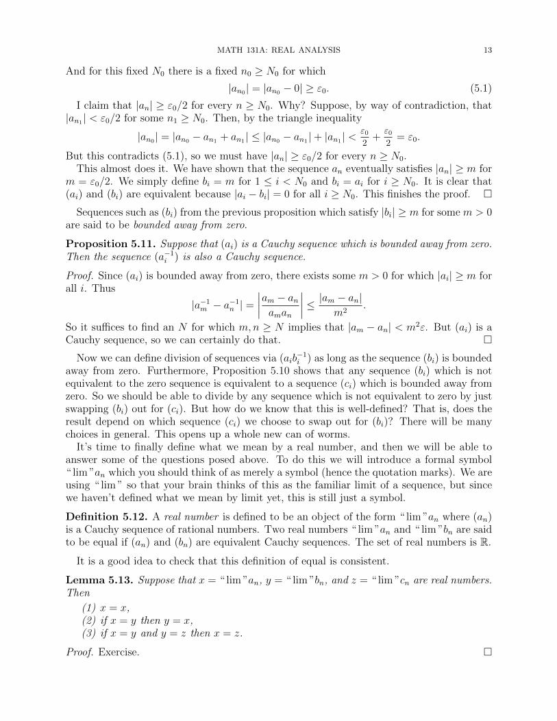
And for this fixed N0 there is a fixed n0 ≥ N0 for which
|an0| = |an0 − 0| ≥ ε0. (5.1)
I claim that |an| ≥ ε0/2 for every n ≥ N0. Why? Suppose, by way of contradiction, that|an1| < ε0/2 for some n1 ≥ N0. Then, by the triangle inequality
|an0| = |an0 − an1 + an1| ≤ |an0 − an1|+ |an1| <ε02
+ε02
= ε0.
But this contradicts (5.1), so we must have |an| ≥ ε0/2 for every n ≥ N0.This almost does it. We have shown that the sequence an eventually satisfies |an| ≥ m for
m = ε0/2. We simply define bi = m for 1 ≤ i < N0 and bi = ai for i ≥ N0. It is clear that(ai) and (bi) are equivalent because |ai − bi| = 0 for all i ≥ N0. This finishes the proof. �
Sequences such as (bi) from the previous proposition which satisfy |bi| ≥ m for some m > 0are said to be bounded away from zero.
Proposition 5.11. Suppose that (ai) is a Cauchy sequence which is bounded away from zero.Then the sequence (a−1i ) is also a Cauchy sequence.
Proof. Since (ai) is bounded away from zero, there exists some m > 0 for which |ai| ≥ m forall i. Thus
|a−1m − a−1n | =∣∣∣∣am − anaman
∣∣∣∣ ≤ |am − an|m2.
So it suffices to find an N for which m,n ≥ N implies that |am − an| < m2ε. But (ai) is aCauchy sequence, so we can certainly do that. �
Now we can define division of sequences via (aib−1i ) as long as the sequence (bi) is bounded
away from zero. Furthermore, Proposition 5.10 shows that any sequence (bi) which is notequivalent to the zero sequence is equivalent to a sequence (ci) which is bounded away fromzero. So we should be able to divide by any sequence which is not equivalent to zero by justswapping (bi) out for (ci). But how do we know that this is well-defined? That is, does theresult depend on which sequence (ci) we choose to swap out for (bi)? There will be manychoices in general. This opens up a whole new can of worms.
It’s time to finally define what we mean by a real number, and then we will be able toanswer some of the questions posed above. To do this we will introduce a formal symbol“ lim ”an which you should think of as merely a symbol (hence the quotation marks). We areusing “ lim ” so that your brain thinks of this as the familiar limit of a sequence, but sincewe haven’t defined what we mean by limit yet, this is still just a symbol.
Definition 5.12. A real number is defined to be an object of the form “ lim ”an where (an)is a Cauchy sequence of rational numbers. Two real numbers “ lim ”an and “ lim ”bn are saidto be equal if (an) and (bn) are equivalent Cauchy sequences. The set of real numbers is R.
It is a good idea to check that this definition of equal is consistent.
Lemma 5.13. Suppose that x = “ lim ”an, y = “ lim ”bn, and z = “ lim ”cn are real numbers.Then
(1) x = x,(2) if x = y then y = x,(3) if x = y and y = z then x = z.
Proof. Exercise. �
14 NICKOLAS ANDERSEN
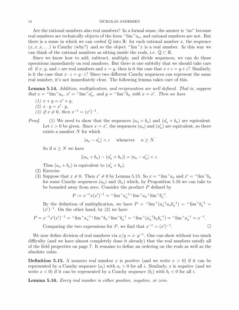
Are the rational numbers also real numbers? In a formal sense, the answer is “no” becausereal numbers are technically objects of the form “ lim ”an, and rational numbers are not. Butthere is a sense in which we can embed Q into R: for each rational number x, the sequence(x, x, x, . . .) is Cauchy (why?) and so the object “ lim ”x is a real number. In this way wecan think of the rational numbers as sitting inside the reals, i.e. Q ⊂ R.
Since we know how to add, subtract, multiply, and divide sequences, we can do thoseoperations immediately on real numbers. But there is one subtelty that we should take careof: if x, y, and z are real numbers and x = y, then is it the case that x+z = y+z? Similarly,is it the case that x · z = y · z? Since two different Cauchy sequences can represent the samereal number, it’s not immediately clear. The following lemma takes care of this.
Lemma 5.14. Addition, multiplication, and reciprocation are well defined. That is, supposethat x = “ lim ”an, x′ = “ lim ”a′n, and y = “ lim ”bn with x = x′. Then we have
(1) x+ y = x′ + y,(2) x · y = x′ · y,(3) if x 6= 0, then x−1 = (x′)−1.
Proof. (1) We need to show that the sequences (an + bn) and (a′n + bn) are equivalent.Let ε > 0 be given. Since x = x′, the sequences (an) and (a′n) are equivalent, so thereexists a number N for which
|an − a′n| < ε whenever n ≥ N.
So if n ≥ N we have
|(an + bn)− (a′n + bn)| = |an − a′n| < ε.
Thus (an + bn) is equivalent to (a′n + bn).(2) Exercise.(3) Suppose that x 6= 0. Then x′ 6= 0 by Lemma 5.13. So x = “ lim ”an and x′ = “ lim ”bn
for some Cauchy sequences (an) and (bn) which, by Proposition 5.10 we can take tobe bounded away from zero. Consider the product P defined by
P := x−1x(x′)−1 = “ lim ”a−1n “ lim ”an“ lim ”b−1n .
By the definition of multiplication, we have P = “ lim ”(a−1n anb−1n ) = “ lim ”b−1n =
(x′)−1. On the other hand, by (2) we have
P = x−1x′(x′)−1 = “ lim ”a−1n “ lim ”bn“ lim ”b−1n = “ lim ”(a−1n bnb−1n ) = “ lim ”a−1n = x−1.
Comparing the two expressions for P , we find that x−1 = (x′)−1. �
We now define division of real numbers via x/y = x ·y−1. One can show without too muchdifficulty (and we have almost completely done it already) that the real numbers satsify allof the field properties on page 7. It remains to define an ordering on the reals as well as theabsolute value.
Definition 5.15. A nonzero real number x is positive (and we write x > 0) if it can berepresented by a Cauchy sequence (ai) with ai > 0 for all i. Similarly, x is negative (and wewrite x < 0) if it can be represented by a Cauchy sequence (bi) with bi < 0 for all i.
Lemma 5.16. Every real number is either positive, negative, or zero.
MATH 131A: REAL ANALYSIS 15
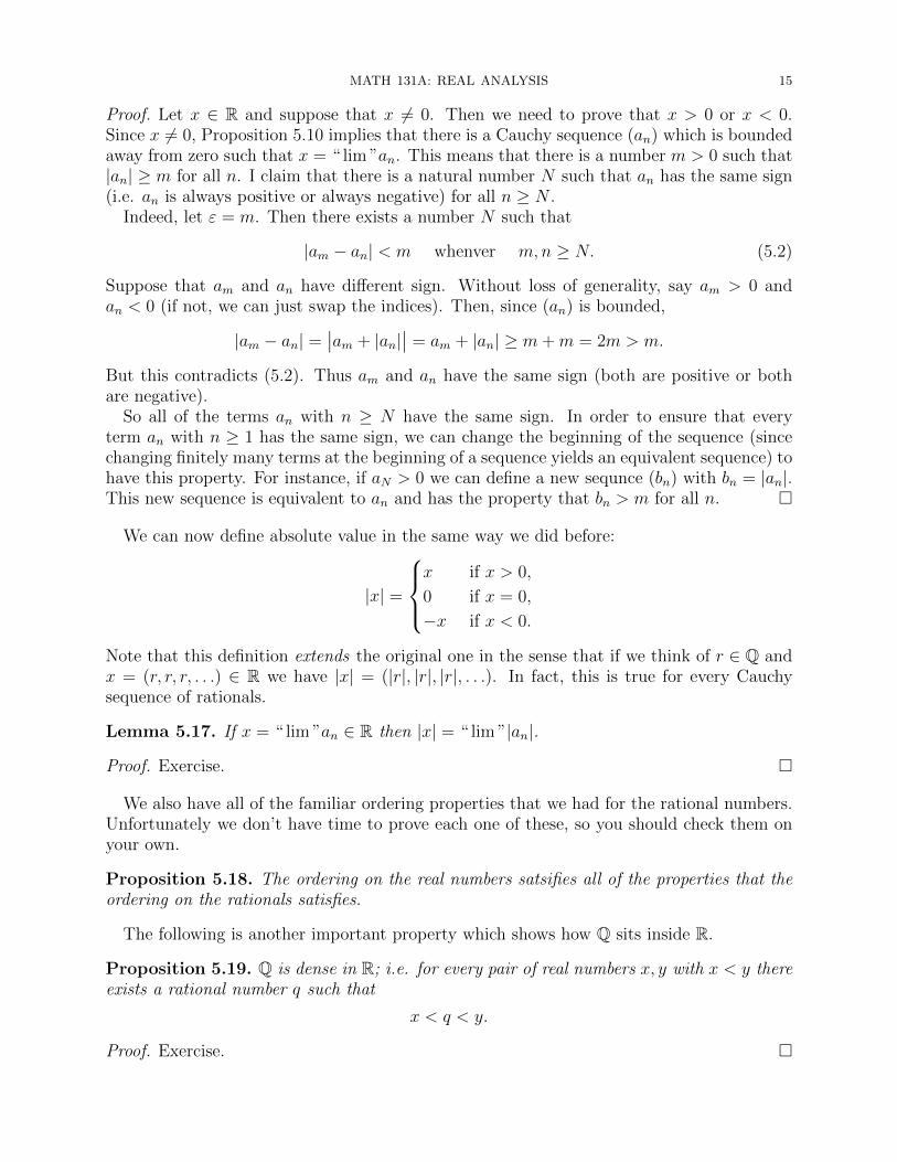
Proof. Let x ∈ R and suppose that x 6= 0. Then we need to prove that x > 0 or x < 0.Since x 6= 0, Proposition 5.10 implies that there is a Cauchy sequence (an) which is boundedaway from zero such that x = “ lim ”an. This means that there is a number m > 0 such that|an| ≥ m for all n. I claim that there is a natural number N such that an has the same sign(i.e. an is always positive or always negative) for all n ≥ N .
Indeed, let ε = m. Then there exists a number N such that
|am − an| < m whenver m,n ≥ N. (5.2)
Suppose that am and an have different sign. Without loss of generality, say am > 0 andan < 0 (if not, we can just swap the indices). Then, since (an) is bounded,
|am − an| =∣∣am + |an|
∣∣ = am + |an| ≥ m+m = 2m > m.
But this contradicts (5.2). Thus am and an have the same sign (both are positive or bothare negative).
So all of the terms an with n ≥ N have the same sign. In order to ensure that everyterm an with n ≥ 1 has the same sign, we can change the beginning of the sequence (sincechanging finitely many terms at the beginning of a sequence yields an equivalent sequence) tohave this property. For instance, if aN > 0 we can define a new sequnce (bn) with bn = |an|.This new sequence is equivalent to an and has the property that bn > m for all n. �
We can now define absolute value in the same way we did before:
|x| =
x if x > 0,
0 if x = 0,
−x if x < 0.
Note that this definition extends the original one in the sense that if we think of r ∈ Q andx = (r, r, r, . . .) ∈ R we have |x| = (|r|, |r|, |r|, . . .). In fact, this is true for every Cauchysequence of rationals.
Lemma 5.17. If x = “ lim ”an ∈ R then |x| = “ lim ”|an|.
Proof. Exercise. �
We also have all of the familiar ordering properties that we had for the rational numbers.Unfortunately we don’t have time to prove each one of these, so you should check them onyour own.
Proposition 5.18. The ordering on the real numbers satsifies all of the properties that theordering on the rationals satisfies.
The following is another important property which shows how Q sits inside R.
Proposition 5.19. Q is dense in R; i.e. for every pair of real numbers x, y with x < y thereexists a rational number q such that
x < q < y.
Proof. Exercise. �
16 NICKOLAS ANDERSEN
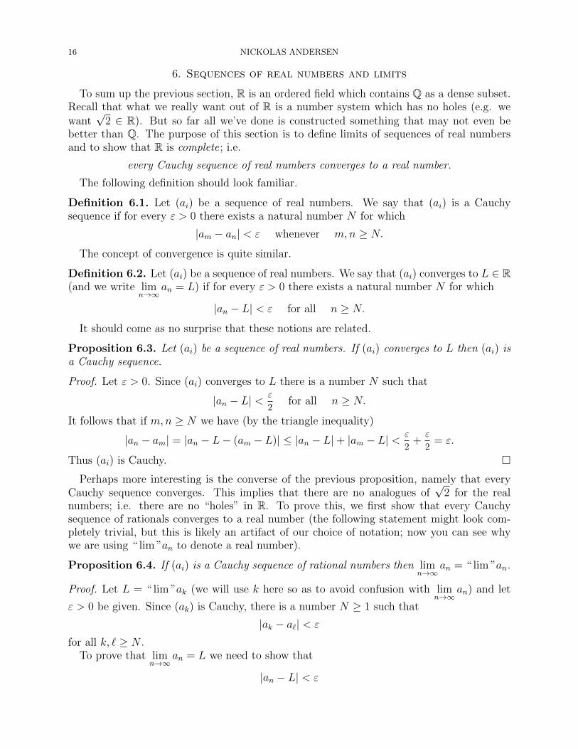
6. Sequences of real numbers and limits
To sum up the previous section, R is an ordered field which contains Q as a dense subset.Recall that what we really want out of R is a number system which has no holes (e.g. wewant
√2 ∈ R). But so far all we’ve done is constructed something that may not even be
better than Q. The purpose of this section is to define limits of sequences of real numbersand to show that R is complete; i.e.
every Cauchy sequence of real numbers converges to a real number.
The following definition should look familiar.
Definition 6.1. Let (ai) be a sequence of real numbers. We say that (ai) is a Cauchysequence if for every ε > 0 there exists a natural number N for which
|am − an| < ε whenever m,n ≥ N.
The concept of convergence is quite similar.
Definition 6.2. Let (ai) be a sequence of real numbers. We say that (ai) converges to L ∈ R(and we write lim
n→∞an = L) if for every ε > 0 there exists a natural number N for which
|an − L| < ε for all n ≥ N.
It should come as no surprise that these notions are related.
Proposition 6.3. Let (ai) be a sequence of real numbers. If (ai) converges to L then (ai) isa Cauchy sequence.
Proof. Let ε > 0. Since (ai) converges to L there is a number N such that
|an − L| <ε
2for all n ≥ N.
It follows that if m,n ≥ N we have (by the triangle inequality)
|an − am| = |an − L− (am − L)| ≤ |an − L|+ |am − L| <ε
2+
ε
2= ε.
Thus (ai) is Cauchy. �
Perhaps more interesting is the converse of the previous proposition, namely that everyCauchy sequence converges. This implies that there are no analogues of
√2 for the real
numbers; i.e. there are no “holes” in R. To prove this, we first show that every Cauchysequence of rationals converges to a real number (the following statement might look com-pletely trivial, but this is likely an artifact of our choice of notation; now you can see whywe are using “ lim ”an to denote a real number).
Proposition 6.4. If (ai) is a Cauchy sequence of rational numbers then limn→∞
an = “ lim ”an.
Proof. Let L = “ lim ”ak (we will use k here so as to avoid confusion with limn→∞
an) and let
ε > 0 be given. Since (ak) is Cauchy, there is a number N ≥ 1 such that
|ak − a`| < ε
for all k, ` ≥ N .To prove that lim
n→∞an = L we need to show that
|an − L| < ε
MATH 131A: REAL ANALYSIS 17
for sufficiently large n (say n ≥ N). Let’s think about what this means: the real numberan − L is the difference of the rational number an and the real number L. To add/subtractreal numbers, we need to represent each one by a Cauchy sequence. This is already done forL, and for an we can use the constant sequence (an, an, an, . . .). Thus
|an − L| = |“ lim ”(an, an, an, . . .)− “ lim ”(a1, a2, a3, . . . , ak, . . .)|= |“ lim ”(an − a1, an − a2, . . . , an − ak, . . .)|= “ lim ”(|an − a1|, |an − a2|, . . . , |an − ak|, . . .),
where we have use Lemma 5.17 in the last step. For all k ≥ N we have
|an − ak| < ε,
so the real number |an − L| is less than ε (think carefully about why this is). Thereforelimn→∞
an = L. �
We can now prove that R is complete.
Theorem 6.5. R is complete. Equivalently, every Cauchy sequence of real numbers con-verges to a real number.
Proof. Suppose that (xn) is a Cauchy sequence of real numbers. Let ε > 0 be given. Foreach n, choose a rational number qn such that
|xn − qn| <ε
3.
This is possible because Q is dense in R. Then the sequence (qn) is Cauchy because
|qm − qn| = |qm − xm + xm − xn + xn − qn| ≤ |qm − xm|+ |xm − xn|+ |xn − qn|and form,n sufficiently large this quantity is less than ε because we can make |xm−xn| < ε/3.
Let L = “ lim ”qn. We will show that limn→∞
xn = L. Let ε > 0 be given. By the previous
proposition, (qn) converges to L, so there is some N ≥ 1 such that
|qn − L| <ε
2
for all n ≥ N . It follows that
|xn − L| = |xn − qn + qn − L| ≤ |xn − qn|+ |qn − L| <ε
3+
ε
2< ε
for all n ≥ N , as desired. �
We conclude this section by listing some additional properties of convergent sequences.First, since convergent sequences are Cauchy, we can extend the properties of Cauchy se-quences of rational numbers to convergent sequences of real numbers (via essentially thesame proofs). In particular, we have the following.
Proposition 6.6. Every convergent sequence of real numbers is bounded.
Is the converse true? That is, is every bounded sequence convergent? Here is a quickcounterexample: consider the sequence 1, 0, 1, 0, 1, 0, 1, 0, . . .. This sequence is bounded be-cause |an| ≤ 1 for all n, but it is clearly not convergent. However, it is the case that boundedmonotonic sequences are convergent. There are two versions of this: increasing sequenceswhich are bounded above are convergent, and decreasing sequences which are bounded beloware convergent. We will state and prove the first version in the next section.
18 NICKOLAS ANDERSEN
We can also do arithmetic with limits. One way to prove the following properties is toreplace every convergent sequence of reals with a convergent sequence of rationals that hasthe same limit (see the proof of the previous theorem). Then arithmetic of limits is the sameas arithmetic of real numbers of the form “ lim ”an, which we have already covered.
Proposition 6.7. Suppose that (an) and (bn) are convergent sequences of real numbers.Then the following are true.
(1) limn→∞
(an + bn) = limn→∞
an + limn→∞
bn
(2) limn→∞
(anbn) = limn→∞
an limn→∞
bn
(3) if c ∈ R then limn→∞
can = c limn→∞
an
(4) if bn 6= 0 for all n and if limn→∞
bn 6= 0 then limn→∞
anbn
=limn→∞
an
limn→∞
bn
The following proposition gives a list of basic limits which will come in handy later on.See Theorem 9.7 in your book for a proof.
Proposition 6.8. The following are true.
(1) If p > 0 then limn→∞
1np = 0.
(2) If |a| < 1 then limn→∞
an = 0. If a = 1 then limn→∞
an = 1. If a = −1 or if |a| ≥ 1 then
the sequence (an) does not converge.(3) If a > 0 then lim
n→∞a1/n = 1.
Finally, the ordering on the reals plays nicely with limits, too. We will frequently use thisproperty without stating it.
Lemma 6.9. Suppose that (an) is a convergent sequence. If an ≤M for all n ≥ 1 then
limn→∞
an ≤M.
Similarly, if an ≥ m for all n ≥ 1 then
limn→∞
an ≥ m.
Proof. Exercise. �
7. The least upper bound property
We constructed the real numbers by filling in the holes in the rational numbers. But oneother advantange to the reals over the rationals is the existence of a least upper bound forany subset of the real numbers. (Your textbook [2] treats this property as an axiom; see §4,p. 23. We will show that it follows from the completeness of the real numbers.)
Definition 7.1. Suppose that E ⊆ R is a set of real numbers and let M,m ∈ R. We saythat M is an upper bound for E if x ≤M for every x ∈ E. Similarly, m is a lower bound forE if x ≥ m for every x ∈ E.
MATH 131A: REAL ANALYSIS 19
Consider the interval E = [0, 1] = {x ∈ R : 0 ≤ x ≤ 1}. This set has many upper bounds;for example, 1, 2, and 496 are upper bounds. Also 172893
172892is an upper bound. It also has
many lower bounds; for example, 0 and −5. But if I asked you to name an upper bound anda lower bound for E, you would likely say 1 and 0, respectively. This is because these arethe least upper bound and greatest lower bound (and so they tell you the most informationabout the set E).
Definition 7.2. Suppose that E ⊆ R is a set of real numbers and let M,m ∈ R. We saythat M is a least upper bound for E if (a) M is an upper bound for E and (b) if M ′ is anotherupper bound for E, then M ′ ≥M . Similarly, we say that m is a greatest lower bound for Eif (a) m is a lower bound for E and (b) if m′ is another lower bound for E then m′ ≤ m.
It should come as no surprise that least upper bounds are unique.
Proposition 7.3. Suppose that M and M ′ are both least upper bounds for E. Then M = M ′.
Proof. By the definition, since M is a least upper bound and M ′ is another upper bound,we must have M ′ ≥ M . Reversing the roles of M and M ′ (i.e. by symmetry) we find thatM ≥M ′. Thus M = M ′. �
If E has a least upper bound then we write sup(E) for the supremum, or least upper bound,of E. Similarly, if E has a greatest lower bound then we write inf(E) for the infimum, orgreatest lower bound.
One of the most important properties of the real numbers is the existence of a least upperbound for every subset of R that you would expect to have a least upper bound. That is,if a set E doesn’t have an upper bound, then we shouldn’t expect it to have a least upperbound. The proof of this theorem is somewhat involved, and I won’t give all of the details;you should fill these in on your own.
Theorem 7.4. Let E be a non-empty subset of R. If E has an upper bound, then it has aleast upper bound.
Proof. Since E is non-empty, there is some element a1 ∈ E, and since E has an upper bound,we can choose some upper bound b1. Clearly a1 ≤ b1. We will define two sequences (ai) and(bi) inductively such that an ≤ bn for all n.
For each n ≥ 1, suppose that we have constructed an and bn such that an ≤ bn. LetK = an+bn
2be the average of an and bn. Note that an ≤ K ≤ bn. If K is an upper bound
for E, let an+1 = an and let bn+1 = K = an+bn2
. Then |bn+1 − an+1| = |an+bn2− an| = bn−an
2.
If K is not an upper bound for E, then there is some element x ∈ E such that x > K(otherwise K would be an upper bound). In that case, let an+1 = x and let bn+1 = bn. Then|bn+1 − an+1| = bn − x < bn − K = bn−an
2. Note that in either case |bn+1 − an+1| ≤ bn−an
2.
Also in either case an is increasing (or staying the same) and bn is decreasing (or staying thesame).
Since an ∈ E for all n and bn is an upper bound for E for all n, we have
a1 ≤ a2 ≤ a3 ≤ · · · ≤ b3 ≤ b2 ≤ b1.
Using the inequality |bn+1 − an+1| ≤ bn−an2
one can show by induction (check this!) that
|bn+1 − an+1| ≤b1 − a1
2n. (7.1)
We will show that the sequences (an) and (bn) are Cauchy.
20 NICKOLAS ANDERSEN
Let ε > 0 be given. Choose N ≥ 1 such that 2N > b1−a1ε
(why is this possible?). Letm,n ≥ N . Without loss of generality, assume that m ≥ n (otherwise just swap them). Thenam ≥ an, and we have
|am − an| = am − an ≤ bn − an ≤b1 − a1
2n< ε.
Thus (an) is Cauchy. A very similar argument shows that (bn) is Cauchy (check this!).Using (7.1) one can show that (an) and (bn) are equivalent sequences (check this!). There-
fore they have the same limit, say L. I claim that L is the least upper bound of E. Onthe one hand, if x ∈ E then x ≤ bn for all n since every bn is an upper bound for E. Thusx ≤ L. Since x was an arbitrary element of E, we conclude that L is an upper bound for E.On the other hand, if L′ is any other upper bound, then L′ ≥ an for all n since every an isan element of E. Thus L′ ≥ L. It follows that L is the least upper bound of E. �
There is a version of this for lower bounds as well.
Corollary 7.5. Let E be a non-empty subset of R. If E has a lower bound, then it has agreatest lower bound.
Proof. Exercise. �
We can also talk about the supremum and infimum of a sequence. To each sequence (an)we associate the set of numbers E = {an : n ≥ 1}, and we define sup an := supE andinf an := inf E if those quantities exist.
For example, let an = (−1)n; then (an) is the sequence −1, 1,−1, 1,−1, 1, . . .. The asso-ciated set is the two-element set E = {−1, 1}. This has least upper bound 1 and greatestlower bound −1. Thus sup an = 1 and inf an = −1.
As another example, let an = 1/n. Then the sequence is 1, 12, 13, 14, 15, . . . and the set is
E = {1, 12, 13, 14, 15, . . .}. The least upper bound of E is 1 and the greatest lower bound of E
is 0. Note that 0 is not in the set, nor is it in the sequence, but it is the largest number lessthan or equal to every element of the set/sequence.
The existence of a least upper bound for bounded sets implies the existence of a least upperbound for bounded sequences. We will use this fact to prove the following proposition.
Proposition 7.6. Bounded monotonic sequences are convergent. That is, if (an) is a se-quence which satisfies an ≤ M for some M ∈ R, and if an is increasing (an+1 ≥ an for alln) then (an) converges.
Proof. Suppose that (an) is an increasing sequence which is bounded above. Let E be theset of values {an : n ≥ 1}. Then (an) has a least upper bound which we will call s = sup an.We will show that limn→∞ an = s.
Let ε > 0 be given. Since s is the least upper bound, s− ε is not an upper bound for E.So there exists some N ≥ 1 such that aN > s − ε. Since (an) is increasing, it follows thatan ≥ aN > s− ε for all n ≥ N . Thus, for all n ≥ N we have
|an − s| = s− an ≤ s− aN < s− (s− ε) = ε.
Therefore (an) converges to s. �
There is a version of this for decreasing sequences which are bounded below.
Proposition 7.7. If (an) is a sequence which satisfies an ≥ m for some m ∈ R, and if anis decreasing (an+1 ≤ an for all n) then (an) converges.

MATH 131A: REAL ANALYSIS 21
Proof. Exercise. �
8. Subsequences and the Bolzano-Weierstrass theorem
Consider the sequence (an) defined by an = (−1)n. The terms of this sequence are
−1, 1,−1, 1,−1, 1,−1, 1, . . . .
It should be clear that this is not a convergent sequence. But it’s kind of close to beingconvergent in the sense that it seems like the sequence wants to converge to two differentlimits: 1 and −1. In this case we say that there is a subsequence (say, take all of the −1terms) that converges.
Definition 8.1. A subsequence of a sequence (an) is a sequence of the form (ank), where nk
is a strictly increasing sequence of natural numbers.
In plain English, this says that a subsequence is a selection of some (maybe all) of theterms of (an) taken in order. So in our example above, say we take n1 = 2, n2 = 3, n3 = 5,n4 = 6, n5 = 8, and nk = 2k for all k ≥ 6. Then the terms of the subsequence (ank
) is
1,−1,−1, 1, 1, 1, 1, . . . .
Since the terms are all 1 after the fourth term, this subsequence is convergent. See §11 ofthe textbook for more examples of subsequences. The purpose of this section is to prove theBolzano-Weierstrass theorem, which states that every bounded sequence has a convergentsubsequence. We will prove this in a few steps.
Note: we have not explicitly defined what it means for lim an = ±∞, so if you are notalready familiar with this idea, please see Definition 9.8 on p. 50 of your textbook.
Proposition 8.2. Suppose that (an) is a sequence.
(1) Let t ∈ R. There is a subsequence of (an) converging to t if and only if the set
{n ∈ N : |an − t| < ε} (8.1)
is infinite for each ε > 0.(2) If (an) is unbounded above then it has a subsequence with limit +∞.(3) If (an) is unbounded below then it has a subsequence with limit −∞.
In each case, we can take the subsequence to be monotonic.
Proof. (1) (⇒) Suppose that there is a subsequence (ank) converging to t. Then for each
ε > 0 there exists a number N such that
|ank− t| < ε
for every nk ≥ N . Since N is a finite number, there are infinitely many nk ≥ N , so the set(8.1) is infinite.
(⇐) Suppose that, for each ε > 0, the set (8.1) is infinite. There is one special case thatwe should consider first. It might be that an = t for infinitely many t (then certainly (8.1)would be infinite for any ε > 0). But then we can just take the subsequence consisting ofterms with ank
= t and that’s a monotonic convergent subsequence. It’s more interestingwhen that’s not the case.
So suppose that an = t for only finitely many n. Then, for each ε > 0, the set
{n ∈ N : 0 < |an − t| < ε}
22 NICKOLAS ANDERSEN
is infinite. Let’s unpack what this means:
0 < |an − t| < ε if and only if 0 < an − t < ε or − ε < an − t < 0.
The last two inequalities can be written
t < an < t+ ε or t− ε < an < t.
Let
S−(ε) := {n ∈ N : t− ε < an < t} and S+(ε) := {n ∈ N : t < an < t+ ε}.
Note that if ε2 ≤ ε1 then S±(ε2) ⊆ S±(ε1) (think about this carefully until you are convinced).It follows that one of the following two statements is true (both could be true):
S+(ε) is infinite for every ε > 0 (8.2)
or
S−(ε) is infinite for every ε > 0. (8.3)
Let us assume that (8.2) is true. The proof in the case that (8.3) holds is quite similar(and is the case your book covers). We will construct a sequence n1, n2, n3, n4, . . . in a similarway as in the proof of Theorem 7.4. Since S+(1) is infinite, there exists some n1 ∈ S+(1).For this n1 we have
t < an1 < t+ 1.
Now suppose we have chosen n1 through nk such that n1 < n2 < n3 < · · · < nk and suchthat
t < anj≤ min{t+ 1
j, anj−1
} for j = 1, 2, 3, . . . , k.
(We use the min so that the subsequence ankis decreasing.) With ε1 = 1
k+1we can use
that S+(ε1) is infinite to find the next index nk+1. But we also want this minimum propertyto hold. So write ank
= t + (ank− t). Since ank
> t the number ε2 = ank− t is positive.
So the set S+(ε2) is infinite. Taking ε to be the smaller of ε1, ε2 we can find some numbernk+1 ∈ S+(ε) such that nk+1 > nk and
t < ank+1≤ min{t+ 1
k+1, ank}.
Thus we have constructed a subsequence (ank) which is decreasing and bounded below (and
therefore convergent).The proofs of (2) and (3) are much easier; see the proof of Theorem 11.2 in your book if
you are interested. �
As an example of what we can do with this proposition, let’s prove that every sequence ofpositive numbers with inf an = 0 has a subsequence converging to 0. (Can you write down anexample of a sequence such that inf an = 0 but (an) is not convergent?) By the proposition,it suffices to show that the sets {n ∈ N : an < ε} are infinite for each ε > 0. Suppose, byway of contradiction, that there is some ε0 > 0 such that an < ε0 for only finitely manyn. Then inf an = min{an : an < ε0} (think carefully about why this is). But each an ispositive, so this means that inf an > 0, a contradiction. So there must exist a subsequence(ank
) converging to 0.
Proposition 8.3. If the sequence (an) converges, then every subsequence converges to thesame limit.
MATH 131A: REAL ANALYSIS 23
Proof. This is pretty straightforward. Let (ank) be a subsequence of (an). Note that nk ≥ k
for all k ≥ 1 (convince yourself that this is true or look in Theorem 11.3 in your book for aninductive justification). Let L = lim an. Then for each ε > 0 there is some N ≥ 1 such that|an −L| < ε. Thus, for k ≥ N we have nk ≥ k ≥ N , which implies that |ank
−L| < ε. Thus(ank
) converges to L. �
We are almost ready to prove Bolzano-Weierstrass, but first we need one more intermediateresult.
Proposition 8.4. Every sequence has a monotonic subsequence.
Proof. Let (an) be a sequence. For the purposes of this proof, let’s say that a term an isdominant if it is larger than every term after it:
an > am for all m > n.
If there are infinitely many dominant terms, let (ank) be the subsequence consisting of all
the dominant terms. Then (ank) is decreasing.
Now suppose that there are only finitely many dominant terms. Then we can choose n1
such that an1 is after every dominant term. Then for every k ≥ 2, choose nk such thatnk > nk−1 and ank
≥ ank−1. Why can we always do this? Because if we couldn’t, then there
would be another dominant term; but we started after all the dominant terms. So we haveconstructed an increasing subsequence (ank
). �
Our main theorem now follows quickly.
Theorem 8.5 (Bolzano-Weierstrass). Every bounded sequence has a convergent subsequence.
Proof. Let (an) be a bounded sequence. By Proposition 8.4 there is a monotonic subsequence(ank
). This subsequence is clearly also bounded, so it is convergent. �
As an example, consider the sequence (an) defined by an = cos(πn3
). The terms of thissequence are
1
2,−1
2,−1,−1
2,1
2, 1, . . . .
This is a bounded sequence, so it contains a convergent subsequence. For example, we cantake the constant subsequences consisting of all terms of the form 1
2, or −1
2, or −1, or 1.
Actually, this example illustrates an important idea: the values 12,−1
2, 1,−1 are called the
limit points of the sequence (an). We will discuss this more in the next section.
9. lim sup and lim inf
Definition 9.1. Let (an) be a sequence. A limit point of (an) is any real number (or symbol±∞) that is the limit of some subsequence (an). Sometimes limit points are referred toas cluster points or accumulation points or condensation points, and your book calls themsubsequential limits. I think that the term limit point is used most throughout mathematics,so we will use it here.
If (an) is a convergent sequence, then since all subsequences converge to the same limit(say, L), the set of all limit points of (an) is just {L}. There are several examples of limitpoints on p. 73 of your book.
24 NICKOLAS ANDERSEN
There are two particularly important limit points for any sequence, called the lim sup andthe lim inf. These are defined as
lim sup an = limN→∞
sup{an : n > N},
lim inf an = limN→∞
inf{an : n > N}.
We allow lim sup an = +∞ and lim inf an = −∞. Note that lim sup an is not necessarily thesupremum of the set {an : n ∈ N}, but it is the largest value that infinitely many of theterms an get close to. The following proposition shows that for convergent sequences, thelim inf and the lim sup are equal. We will not prove it here, but a proof is given in Theorem10.7 of your book.
Proposition 9.2. If (an) is a convergent sequence then
lim inf an = limn→∞
an = lim sup an.
Now let’s see how limit points and lim sup / lim inf are related.
Proposition 9.3. Let (an) be a sequence. There exists a monotonic subsequence whose limitis lim sup an and a monotonic sequence whose limit is lim inf an.
Proof. If (an) is unbounded above or below, then we just apply Proposition 8.2 part (2) or(3). So suppose that (an) is bounded either above or below (actually let’s just pick one sincethe other case is similar). Suppose that (an) is bounded above, then t = lim sup an is a finitenumber. Let ε > 0. Then there exists N ≥ 1 such that (by definition of lim sup)
| sup{an : n > N} − t| < ε.
But the sup is larger than or equal to t, so we can say that
sup{an : n > N} < t+ ε.
In particular, an < t+ ε for all n > N (since an ≤ sup{an : n > N}). I claim that the set
{n ∈ N : |an − t| < ε} (9.1)
is infinite. If not, then for some N ′ we have an ≤ t − ε for all n ≥ N ′. But this meansthat lim sup an < t, a contradiction. So the set (9.1) is infinite; by Proposition 8.2 there is amonotonic subsequence of (an) converging to t = lim sup an. �
As an immediate consequence of the previous proposition, we see that the set of limitpoints of any sequence (an) contains at least one element (both the lim sup and lim inf arein the set, but they might be equal). Not only that, but it turns out that lim sup an is thesupremum of the set of limit points (and similarly with the lim inf). See Theorem 11.8 ofyour book for a proof of this last fact. Also see p. 75 for some examples.
There are more properties of lim sup and lim inf in §12 of your book, but we will not needthem here (and if we need them later, we will come back and prove them).
10. Series
When you saw sequences and series in your Calculus courses previously, you likely spentvery little time talking about sequences and a lot of time talking about series. Maybe,because of this, you think of series as being “more complicated” than sequences. However,since we have taken such a long time carefully building up the theory of sequences and limits,
MATH 131A: REAL ANALYSIS 25
it turns out that we can prove many results about series very quickly. But first we need somerigorous definitions.
Definition 10.1. An infinite series is an object of the form∞∑k=1
ak (10.1)
where (ak) is a sequence of real numbers. To give a precise meaning to (10.1), for each n ≥ 1let
sn =n∑k=1
ak = a1 + a2 + . . .+ an
be the nth partial sum. We say that (10.1) converges if the sequence (sn) is a convergentsequence. In this case, if S = lim sn, we write
∞∑k=1
ak = S.
If the sequence of partial sums is not convergent, then we say the series diverges. Sometimeswe can be more precise about how it diverges by saying that it diverges to +∞ if lim sn = +∞and that it diverges to −∞ if lim sn = −∞. Lastly, if
∑|an| is convergent, we say the series∑
an is absolutely convergent.
Note: above I have written the series as starting with the index k = 1. In fact wecan start at any index k = m and modify the definition appropriately by defining sn =am + am+1 + . . . + an. Often it will not matter where the index begins, and so I will justwrite
∑an for a “generic” series.
By transferring what we know about sequences to series, we can prove some very usefulresults without too much effort. We’ll start by using the fact that a sequence converges ifand only if it is Cauchy. We say that a series satsifies the Cauchy criterion if its sequenceof partial sums is Cauchy, and we immediately get the following proposition.
Proposition 10.2 (Cauchy criterion). A series∑an is convergent if and only if for each
ε > 0 there exists a number N ≥ 1 such that∣∣∣∣∣n∑
k=m
ak
∣∣∣∣∣ < ε
whenever n ≥ m ≥ N .
From this we (almost) immediately get the following familiar corollary.
Corollary 10.3. If∑an is convergent then lim
n→∞an = 0.
Proof. Apply the Cauchy criterion with m = n to get: for every ε > 0 there exists a numberN ≥ 1 such that |an| < ε whenever n ≥ N . �
You may be more familiar with the previous corollary under the name “the divergencetest.” Indeed, one (usually easy) way to check if a series diverges is to check whether itsterms go to zero or not. If not, then the series diverges. Of course, even if the terms do goto zero, that’s not a guarantee that the series converges.
26 NICKOLAS ANDERSEN
We can also do arithmetic on series (addition and multiplication by a constant) by applyingthe limit laws for sequences: if
∑an and
∑bn are both convergent then∑
(an + bn) =∑
an +∑
bn
and if∑an is convergent and c is any constant then∑
can = c∑
an.
In order to determine the convergence of a given series, it is often useful to compare it toanother “simpler” series which you already know converges or diverges. Two such “simple”series are the geometric series and the p-series.
A geometric series is a series of the form∑arn for some constant a and some constant
ratio r. Since we can always pull out the constant a, we will only need to think aboutgeometric series of the form
∑rn.
Proposition 10.4. If |r| < 1 then the geometric series∑rn is absolutely convergent; fur-
thermore,∞∑n=0
rn =1
1− r. (10.2)
If |r| ≥ 1 then∑rn diverges.
Proof. It is not too hard to show by induction (try it!) that for any r 6= 1 we havem∑n=0
rn =1− rm
1− r.
(If r = 1 then it is clear that the series diverges.) By the limit laws, it follows that the seriesconverges if and only if lim
m→∞rm is finite, which is true if and only if |r| < 1. In that case,
we have limm→∞
rm = 0, which proves equation (10.2). Finally, if |r| < 1 then∑|rn| =
∑|r|n
is convergent, so∑rn is absolutely convergent. �
A p-series is a series of the form∑
1np for some fixed p. We already showed that for p = 1,
this series is divergent (this was way back when we first learned about Cauchy sequences; seeProposition 5.4). Since this case is so important and is used as a counterexample to manytheorems in analysis, let’s give it its own proposition.
Proposition 10.5. The harmonic series∑
1n
is divergent.
What happens for other values of p? It turns out that the harmonic series is the dividingline between convergent p-series and divergent p-series, as the next proposition shows.
Proposition 10.6. If p ≤ 1 then the p-series∑
1np diverges. If p > 1 then it converges.
This is usually proved using the integral test, but since we haven’t covered integrals yet,we’re going to use a different method. We will, however, need to prove the comparison testfirst.
Proposition 10.7 (The comparison test). Let∑an be a series of nonnegative terms (an ≥ 0
for all n).
(1) If∑an converges and |bn| ≤ an for all n then
∑bn converges.
(2) If∑an = +∞ and bn ≥ an for all n then
∑bn diverges.
MATH 131A: REAL ANALYSIS 27
Proof. (1) Suppose that∑an converges. Then it satisfies the Cauchy criterion. Given ε > 0
there exists a number N ≥ 1 such thatm∑k=n
ak =
∣∣∣∣∣m∑k=n
ak
∣∣∣∣∣ < ε
for all n ≥ m ≥ N (note ak ≥ 0 for all k). So for m ≥ n ≥ N we have∣∣∣∣∣m∑k=n
bk
∣∣∣∣∣ ≤m∑k=n
|bk| ≤m∑k=n
ak < ε,
where we used the Triangle inequality in the first step. Thus∑bn satisfies the Cauchy
criterion, and therefore it converges.(2) Let (sn) be the sequence of partial sums for
∑an and let (tn) be the sequence of partial
sums for∑bn. Then tn ≥ sn for all n. Since lim sn = +∞ we have lim tn = +∞ too. �
Before we prove Proposition 10.6, I should mention a quick corollary of the comparisontest which you are likely familiar with.
Corollary 10.8. Absolutely convergent series are convergent.
Proof. Suppose that∑bn is absolutely convergent. Then
∑|bn| converges. Since (trivially)
|bn| ≤ |bn|, the comparison test says that∑bn converges. �
Now we can prove Proposition 10.6.
Proof of Proposition 10.6. Suppose first that p ≤ 1. Then 1np ≥ 1
nfor all n ≥ 1. By the
comparison test,∑
1np diverges.
Now suppose that p > 1. Let (sn(p)) denote the sequence of partial sums, i.e.
sn(p) =n∑k=1
1
np= 1 +
1
2p+
1
3p+ · · ·+ 1
np.
Consider the 2n-th partial sum and split into even and odd terms:
s2n(p) = 1 +
(1
2p+
1
4p+
1
6p+ · · ·+ 1
(2n)p
)+
(1
3p+
1
5p+
1
7p+ · · ·+ 1
(2n− 1)p
).
Since 3p > 2p and 5p > 4p and 7p > 6p, etc. we have
s2n(p) < 1 + 2
(1
2p+
1
4p+
1
6p+ · · ·+ 1
(2n)p
)= 1 +
2
2p
(1
1p+
1
2p+
1
3p+ · · ·+ 1
np
)= 1 +
2
2psn(p).
Since (sn(p)) is an increasing sequence (we are adding positive terms every time) we have
sn(p) < 1 +2
2psn(p).
Solving this inequality for sn(p) yields
sn(p) <
(1− 2
2p
)−1.
28 NICKOLAS ANDERSEN
Thus (sn(p)) is an increasing sequence which is bounded above. Therefore it converges. �
We will only talk about one more convergence test before we finish our discussion of series.You probably remember several other convergence tests from previous calculus courses; theseare certainly interesting, but won’t help us much in our ultimate goal for this course. If youare interested in learning more about infinite series, I suggest you take a course in complexanalysis or analytic number theory.
Proposition 10.9 (Alternating series test). If (an) is a decreasing sequence (an+1 ≤ an) ofnonnegative real numbers (an ≥ 0) and lim an = 0 then the alternating series
∑(−1)n+1an
converges.
Proof. Let (sn) denote the sequence of partial sums. Let (en) be the subsequence of even-indexed terms and (on) the subseqeunce of odd-indexed terms. Then on = s2n−1 and en = s2n:
(sn) = o1, e1, o2, e2, o3, e3, . . . .
The even-indexed terms are increasing since
en+1 − en = s2n+2 − s2n = −a2n+2 + a2n+1 ≥ 0.
Similarly, the odd-indexed terms are decreasing since
on+1 − on = s2n+1 − s2n−1 = a2n+1 − a2n ≤ 0.
I claim that every even-indexed term is less than or equal to every odd-indexed term:
em ≤ on for all m,n ∈ N.
First, en ≤ on+1 ≤ on because on+1 − en = s2n+1 − s2n = a2n+1 ≥ 0 and (on) is decreasing.Now, if m ≤ n, then because (en) is increasing, em ≤ en ≤ on. On the other hand, if m ≥ nthen on ≥ om ≥ em. To summarize,
e1 ≤ e2 ≤ e3 ≤ · · · ≤ o3 ≤ o2 ≤ o1.
Since (en) is increasing and bounded above, it converges, say to Le. Similarly, (on) converges,say to Lo. But
Lo − Le = limn→∞
on+1 − limn→∞
en = limn→∞
(on+1 − en) = limn→∞
a2n+1 = 0.
Thus Lo = Le. It follows that (sn) converges. �
As an example, the alternating harmonic series∞∑n=1
(−1)n+1
n
converges since ( 1n) is a decreasing sequence and lim 1
n= 0.
11. Continuous functions
We are finally ready to begin what most of you probably think of as calculus. That is,we are going to discuss continuity, limits, derivatives, etc. To do this we will need to havea precise definition of what a function is. (This definition will be precise enough for ourpurposes, but to be totally rigorous we should probably talk about Cartesian products ofsets; we will not do this here.)
MATH 131A: REAL ANALYSIS 29
Definition 11.1. A function is a pair (X, f), where X ⊆ R is the domain and f is a rulewhich specifies the value f(x) for every x ∈ X. We will usually write our functions usingthe notation f : X → Y . This means that to each x ∈ X, f assigns a value f(x) which isan element of the codomain Y . Note: f must make an assignment for every x ∈ X, but itneed not map to every element of Y .
For example, the function f : R→ R given by f(x) = x2 assigns a value to f(x) for everyx ∈ R (the domain) but does not hit every value of the codomain R (just the nonnegativereals). The function g : N → R given by g(x) = x2 is technically a different function (thedomain is not R).
Sometimes, we will just write a function as a rule, e.g. f(x) = 1/x. In this case, thedomain is implicitly understood to be the largest subset of the real numbers for which theassignment is a well-defined real number (in this case the domain is X = {x ∈ R : x 6= 0}).Another example is g(x) =
√x in which case the domain is X = {x ∈ R : x ≥ 0}.
Definition 11.2. Let X ⊆ R. A function f : X → R is continuous at the point a ∈ X if,for every sequence (an) (with an ∈ X) converging to a, the sequence (f(an)) converges tof(a). Put another way, f is continuous at a if
limn→∞
f(an) = f(
limn→∞
an
)for every sequence (an) converges to a.
This definition essentially says that whenever x is close to a, f(x) is close to f(a). Thereis another way to say this which looks more epsilon-y.
Definition 11.3. Let X ⊆ R. A function f : X → R is continuous at the point a ∈ X if,for every ε > 0 there exists a δ > 0 such that
|f(x)− f(a)| < ε whenever x ∈ X and |x− a| < δ.
Is it alright for a mathematical concept to have two definitions? Usually the answer is no;in math, we like to make sure that everything is perfectly well-defined. In this case, sincethere are two defintions for what it means for a function to be continuous, it’s importantthat we show that they give us the same thing, i.e., that every function which satisfiesDefinition 11.2 also satisfies Definition 11.3, and vice versa.
Proposition 11.4. Definitions 11.2 and 11.3 are equivalent.
Proof. Suppose that f : X → R satisfies Definition 11.3 at the point a ∈ X. Let (an) be asequence in X converging to a. Let ε > 0 be given. Then there exists a δ > 0 such that
|f(x)− f(a)| < ε whenever x ∈ X and |x− a| < δ.
Since (an) converges to a, there is a number N ≥ 1 such that
|an − a| < δ
whenever n ≥ N . Thus, n ≥ N we have |f(an)− f(a)| < ε, so (f(an)) converges to f(a).We argue the other direction by contrapositive. Suppose that Definition 11.3 fails for
f : X → R at the point a ∈ X. Then there exists ε > 0 such that for every δ > 0, thereexists a point x ∈ X such that
|x− a| < δ but |f(x)− f(a)| ≥ ε. (11.1)
30 NICKOLAS ANDERSEN
We will use this to construct a sequence (xn) which converges to a but for which (f(xn))does not converge to f(a). For each n ≥ 1 we apply (11.1) with δ = 1
n. Thus, for each n ≥ 1,
there exists a point xn ∈ X such that
|xn − a| <1
nbut |f(xn)− f(a)| ≥ ε.
The sequence (xn) clearly converges to a but the inequality above shows that (f(xn)) doesnot converge to f(a). �
We say that a function f : X → R is continuous on A ⊆ R if f is continuous at everypoint a ∈ A. Similarly, we say that f : X → R is continuous if f is continuous at a for everya ∈ X.
As an example, let’s prove that f(x) =√x is continuous on its domain X = [0,∞). We
can use either definition. Using the sequential definition: given a ∈ X, let (an) be a sequencein X converging to a. Then
limn→∞
f(an) = limn→∞
√an =
√limn→∞
an =√a.
Here we’re using the fact that lim√an =
√lim an which we never actually proved (though
you did use it on that one homework problem). Let’s prove that√x is continuous using the
ε-δ definition.Let a ∈ X. Given ε > 0 let δ = ε
√a (I chose this after looking at the inequalities below,
then I came back and wrote it in). Then for every x ∈ X such that |x− a| < δ we have
|f(x)− f(a)| = |√x−√a| =
∣∣∣∣(√x−√a)(√x+√a)√
x+√a
∣∣∣∣ =|x− a|√x+√a<
ε√a√
x+√a.
Since√x ≥ 0 the latter expression is < ε. Thus f(x) is continuous at x = a. Two things
to note: first, this choice of δ depends on a (that’s fine right now, but later it’s going to beimportant). Second, this doesn’t work if a = 0 (because then δ = 0 and we need δ > 0). Sosuppose that a = 0. Given ε > 0 let δ = ε2. Then for every x ∈ X such that |x− 0| < δ we
have |√x− 0| <
√δ = ε. Thus f(x) is continuous at x = 0.
As another example, consider the function
f(x) =
{x sin(1/x) if x 6= 0,
0 if x = 0.
We will prove that f(x) is continuous at x = 0. Given ε > 0 let δ = ε. Then for all x ∈ Rsuch that |x− 0| < δ we have
|f(x)− f(0)| = |x sin(1/x)| ≤ |x| < δ = ε.
So f(x) is continuous at x = 0.Now let’s look at the function g defined by g(x) = sin(1/x) if x 6= 0 and g(0) = 0. By
looking at the graph of the function g(x) it seems clear that g cannot possibly be continuousat x = 0. Let’s prove that g is discontinuous at x = 0. We will exhibit two sequences (an)and (bn) both converging to 0 for which (g(an)) and (g(bn)) converge to different limits. Let
an =2
π(4n− 3), bn =
1
πn.
Then
g(an) = sin(π(4n− 3)
2
)= sin
(π
2
)= 1 for all n ≥ 1
MATH 131A: REAL ANALYSIS 31
and
g(bn) = sin(πn) = 0 for all n ≥ 1.
Thus g fails to satisfy Definition 11.2 at the point x = 0.One of the easiest ways to tell if a function is continuous is to build it up from simpler
functions which you already know are continuous. Here are some familiar operations onfunctions (f and g are functions and k is a real constant):
f + g: (f + g)(x) = f(x) + g(x)fg: (fg)(x) = f(x)g(x)f/g: (f/g)(x) = f(x)/g(x)kf : (kf)(x) = k · f(x)|f |: (|f |)(x) = |f(x)|
g ◦ f : (g ◦ f)(x) = g(f(x))
Since we have proved a lot of useful properties of limits of sequences, we can get a lot ofthis essentially for free.
Proposition 11.5. Suppose that f, g are continuous at a ∈ R and let k ∈ R be a constant.Then the functions f + g, fg, kf , and f/g (provided g(a) 6= 0) are continuous at a.
Proof. These all follow from the corresponding properties for limits. For example, let (an) beany sequence converging to a. Since f and g are continuous at a, we have limn→∞ f(an) =f(a) and limn→∞ g(an) = g(a). Therefore
limn→∞
(f + g)(an) = limn→∞
(f(an) + g(an)) = limn→∞
f(an) + limn→∞
g(an) = f(a) + g(a).
The others are similar. �
Corollary 11.6. Polynomial functions are continuous on R.
Proof. Polynomials can be built up from the functions xn, n ∈ N by addition and scalar mul-tiples (both continuity-preserving operations). Since multiplication of continuous functionsis continuous, by induction we have that xn is continuous for every n ∈ N (I’ll leave it as anexercise for you to prove the base case, i.e. that f(x) = x is continuous). �
Proposition 11.7. The function f(x) = |x| is continuous on R.
Proof. Let a ∈ R. The statement is clear for a 6= 0 since f(x) = x when x > 0 and f(x) = −xwhen x < 0. So suppose that a = 0. Given ε > 0 let δ = ε. Then, for any x ∈ R such that|x− 0| < δ we have
|f(x)− f(0)| = ||x| − 0| = |x| < δ = ε.
So f(x) is continuous at x = 0, and thus on all of R. �
Proposition 11.8. If f is continuous at x = a and if g is continuous at f(a) then thecomposite function g ◦ f is continuous at a.
Proof. Let (an) be any sequence in the domain of f such that (an) converges to a and f(an) isin the domain of g for all n. Then, since f is continuous at a, the sequence (f(an)) convergesto f(a). Since (f(an)) is a sequence converging to f(a), and since g is continuous at f(a),we conclude that the sequence (g(f(an))) converges to g(f(a)). �
32 NICKOLAS ANDERSEN
The two most important properties of continuous functions are: that continuous functionsattain their maximum and minimum values on closed intervals, and the Intermediate ValueTheorem. I cannot overstate the importance of these results; they are essential to the proofof the Mean Value Theorem (once we get to derivatives), which is a key ingredient in theproof of the Fundamental Theorem of Calculus.
Theorem 11.9. Let f : [a, b] → R be a continuous function. Then f is bounded (i.e. thereexists a real number M such that |f(x)| ≤ M for all x ∈ [a, b]). Furthermore, f attainsits maximum and minimum values on [a, b] (i.e. there exist x0, y0 ∈ [a, b] such that f(x0) ≤f(x) ≤ f(y0) for all x ∈ [a, b]).
Proof. We argue by contradiction. Suppose that f is not bounded on [a, b]. Then for eachn ∈ N there exists a number xn ∈ [a, b] such that |f(xn)| > n. So we get a sequence (xn)which is bounded (it’s always inside [a, b]). By the Bolzano-Weierstrass theorem, there existsa convergent subsequence (xnk
) of (xn), say that lim xnk= L. Then L ∈ [a, b] (why?), so by
assumption f is continuous at L. So we have a sequence (xnk) which converges to L but the
sequence (f(xnk)) doesn’t converge to f(L) (since |f(xnk
)| → +∞). This contradicts thecontinuity of f , so we must have that f is bounded.
Now let M := sup{f(x) : x ∈ [a, b]}. We just proved that M is a finite number. Foreach n ∈ N there exists a number yn ∈ [a, b] such that M − 1
n≤ f(yn) ≤ M (otherwise M
wouldn’t be the sup). By the squeeze theorem, lim f(yn) = M . We aren’t guaranteed that(yn) is a convergent sequence, but it is bounded (always in [a, b]) so Bolzano-Weierstrassgives us a convergent subsequence (ynk
). Say lim ynk= y0. Since f is continuous at y0 we
have
f(y0) = f(lim ynk) = lim f(ynk
) = lim f(yn) = M.
(In the third equality we used that if a sequence is convergent, then every subsequenceconverges to the same limit.) So f attains its maximum M . The assertion for the minimumis similar. �
Theorem 11.10 (Intermediate Value Theorem). Let I ⊆ R be an interval and suppose thatf : I → R is continuous. Let a, b ∈ I such that a < b. Then for every y between f(a) andf(b) (i.e. either f(a) < y < f(b) or f(a) > y > f(b)) there exists at least one x ∈ (a, b) suchthat f(x) = y.
Proof. Assume that f(a) < y < f(b) (the other case is similar). We will construct twosequences (an) and (bn) which converge to x0 such that f(an) is above y and f(bn) is belowy (hence the letters a for above and b for below).
Let S = {x ∈ [a, b] : f(x) < y}. Then S is not empty because a ∈ S. Since S isalso bounded above (by b) it has a least upper bound, say x0 = supS. For each n ∈ N, thenumber x0− 1
nis not an upper bound for S so there exists bn ∈ S such that x0− 1
n< bn ≤ x0.
By the squeeze theorem, lim bn = x0. Since f is continuous and since f(bn) < y we have
f(x0) = f(lim bn) = lim f(bn) ≤ y.
Now for each n ∈ N let an = min{b, x0 + 1n}. Then for each n, an /∈ S so f(an) ≥ y. Again
by the squeeze theorem, lim an = x0 so we have
f(x0) = f(lim an) = lim f(an) ≥ y.
Thus f(x0) = y. �
MATH 131A: REAL ANALYSIS 33
Here’s a neat example of the intermediate value theorem in action. It’s an example ofa fixed point theorem, and it’s quite surprising at first glance that it should even be true(the hypotheses seem pretty weak). Fixed point theorems are ubiquitous in mathematics,especially in analysis and topology.
Let f : [0, 1]→ [0, 1] be a continuous function. Then f has a fixed point; i.e. there existsa point x0 ∈ [0, 1] such that f(x0) = x0.
Proof. This assertion is equivalent to saying that the graph of f crosses the line y = x. Inorder to use the intermediate value theorem, we will “change coordinates” so that the liney = x is “horizontal.” Don’t worry, there’s nothing fancy going on here, but this is a trickthat we will use again several times. Just let g(x) = f(x) − x. Then g is also continuous.Since 0 ≤ f(x) ≤ 1 we have −x ≤ g(x) ≤ 1−x. Thus g(0) ≥ 0 and g(1) ≤ 0. It follows thatthere is some point x0 ∈ [0, 1] such that g(x0) = 0. Of course, at that point we then havef(x0)− x0 = 0, i.e. f(x0) = x0. �
Now let’s go back and think about the two examples above,
f(x) =
{x sin(1/x) if x 6= 0,
0 if x = 0,
and
g(x) =
{sin(1/x) if x 6= 0,
0 if x = 0.
Both of the functions f and g are continuous on the interval (0, 1] since they are built out offunctions which are continuous on that interval (here we are taking for granted that sinx isa continuous function, but we will not prove that in this class). But above we showed thatf(x) is continuous at 0, so we can say that it is continuous on the interval [0, 1]. The functiong(x) is not continuous at 0 (and there is no way to redefine g(0) so that it is continuous at 0because we found two sequences (an) and (bn) converging to 0 such that (g(an)) and (g(bn))converge to different values). So g is not continuous on the interval [0, 1].
What’s the difference between these examples? Why can we define f(0) = 0 and make fcontinuous on [0, 1] but we can’t do the same for g? It turns out that the answer is somethingcalled uniform continuity. In the remainder of this section we will define this term and provethe following proposition.
Proposition 11.11. A function f : (a, b)→ R can be extended to a continuous function on[a, b] if and only if it is uniformly continuous on (a, b).
I should first explain what it means to extend a function from (a, b) to [a, b]. This definitionshould match your intuition about what it should mean for a function to be extended to alarger domain. We say a function f : Y → R is an extension of f : X → R if
X ⊆ Y and f(x) = f(x) for all x ∈ X.
The definition of uniform continuity will look a lot like the definition of continuity, withone important difference. Instead of fixing a point a ∈ X and letting x be a point close to(i.e. within δ of) a, we let x, y both be free to move about in such a way that they remainclose to each other. This difference is similar to the difference between the definition of asequence converging to a number L and the definition of a Cauchy sequence.
34 NICKOLAS ANDERSEN
Definition 11.12. A function f : X → R is uniformly continuous on X if for every ε > 0there exists a δ > 0 such that
|f(x)− f(y)| < ε whenever x, y ∈ X and |x− y| < δ.
In this definition, δ is allowed to depend on ε but it cannot depend on x or y. As anexample consider the function f : [−4, 2]→ R defined by f(x) = x2. Given ε > 0, let δ = �(we’ll figure out in a minute what δ should be). Note that
|f(x)− f(y)| = |x2 − y2| = |x− y| · |x+ y|.
For x, y ∈ [−4, 2] we have |x+ y| ≤ |x|+ |y| ≤ 4 + 4 = 8. Thus
|f(x)− f(y)| = 8|x− y|.
Now let’s choose δ = ε8
so that when |x− y| < δ we have
|f(x)− f(y)| = 8|x− y| < 8δ = ε.
Thus f is uniformly continuous on [−4, 2].The previous example is no accident, as the next proposition shows.
Proposition 11.13. If f is continuous on a closed interval [a, b] then f is uniformly con-tinuous on [a, b].
Proof. We argue by contradiction. Suppose that f is continuous on [a, b] but not uniformlycontinuous on [a, b]. Then there exists ε > 0 such that for every δ > 0 there exist xδ, yδ ∈ [a, b]such that
|xδ − yδ| < δ but |f(xδ)− f(yδ)| ≥ ε.
We will use this to construct sequences (xn) and (yn). For each n, there exist xn, yn ∈ [a, b]such that
|xn − yn| <1
nbut |f(xn)− f(yn)| ≥ ε.
By Bolzano-Weierstrass, since (xn) and (yn) are bounded, they each have convergent sub-sequences (xnk
) and (ynk). Since we chose xn, yn so that |xn − yn| < 1
nwe must have
limxnk= lim ynk
= c, say. Since f is continuous at c, we have
limk→∞
f(xnk) = f(c) = lim
k→∞f(ynk
),
so
limk→∞
(f(xnk)− f(ynk
)) = 0.
But this contradicts that |f(xn) − f(yn)| ≥ ε for all n. Thus f is uniformly continuous onthe interval [a, b]. �
To make the connection between uniformly continuous functions and Cauchy sequenceseven more solid, we have the following proposition.
Proposition 11.14. If f : X → R is uniformly continuous on X and if (an) is a Cauchysequence then (f(an)) is a Cauchy sequence.
Proof. Let (an) be a Cauchy sequence and let ε > 0. Since f is uniformly continuous on X,there exists a δ > 0 such that
|f(x)− f(y)| < ε
MATH 131A: REAL ANALYSIS 35
whenever x, y ∈ X and |x− y| < δ. Since (an) is Cauchy, there exists and N ≥ 1 such that(now we’re thinking of δ as being the ε in the definition of a Cauchy sequence)
|am − an| < δ
for all m,n ≥ N . Thus, for such m,n we have (thinking of x = am and y = an)
|f(am)− f(an)| < ε
so (f(an)) is a Cauchy sequence. �
We can use the previous proposition to prove that g(x) = sin(1/x) is not uniformlycontinous on (0, 1). Consider the Cauchy sequence (an) given by an = 2
πn. Then the first
few values of the sequence (g(an)) are
(g(an)) = 1, 0,−1, 0, 1, 0,−1, 0, . . . .
It should be clear that (g(an)) is not Cauchy, so g is not uniformly continous on (0, 1).We can now prove our main proposition on uniform continuity.
Proposition 11.15. A function f : (a, b)→ R can be extended to a continuous function on[a, b] if and only if it is uniformly continuous on (a, b).
Proof. (⇒) Suppose that f can be extended to a continuous function f : [a, b] → R. Then
by Proposition 11.13 f is uniformly continuous on [a, b]. It follows immediately that f isuniformly continuous on (a, b).
(⇐) Suppose that f is uniformly continuous on (a, b). We must decide how to define f(a)
and f(b) to make f : [a, b]→ R continuous. It suffices to show how to do this for f(a) (since
f(b) is similar). There is really only one reasonable way to define f(a), and it’s as the limitof a sequence:
f(a) = limn→∞
f(an) for any sequence (an) in (a, b) converging to a. (11.2)
There are two immediate issues here: first, how do we even know the limit exists? and second,how do we know that this definition is unambiguous? (i.e. if you pick another sequence (a′n)
converging to a, does that potentially change the definition of f(a)?) We will deal with theseone at a time.
Claim 1: if (an) is a sequence in (a, b) converging to a then the sequence (f(an)) converges.To prove this, note that (an) is a Cauchy sequence, so by Proposition 11.14, (f(an)) is Cauchy,so it converges.
Claim 2: if (an) and (a′n) both converge to a then lim f(an) = lim f(a′n). To prove this,form the sequence (zn) (z is for zipper) via
(zn) = (a1, a′1, a2, a
′2, a3, a
′3, . . .).
It should be clear that lim zn = lim an = lim a′n = a so by Claim 1, lim f(zn) exists. But now(f(an)) and (f(a′n)) are subsequences of the convergent sequence (f(zn)) so they convergeto the same limit, i.e. lim f(an) = lim f(a′n).
Now that these claims are proven, the definition (11.2) makes sense, and it should also
be clear that f is continous at a (we forced it to be continuous there by defining f(a) to beequal to the limit of (f(an)) for every sequence (an) converging to a). �

36 NICKOLAS ANDERSEN
12. Limits of functions
In our proof of Proposition 11.15 we extended the function f : (a, b)→ R to a continuousfunction on [a, b] by defining
f(a) = limn→∞
f(an) for any sequence (an) in (a, b) converging to a.
One way to think of this is that f(a) is the value that f “wants” to take at x = a, i.e. the
behavior of f near x = a is what determines the value of f(a). This is essentially the ideabehind limits of functions. We will start by defining left-hand and right-hand limits, thenwe’ll define the usual (two-sided) limit.
Definition 12.1. Let f : X → R be a function and let a ∈ X. Suppose that X containsthe interval (a, b) for some b > a. We say that lim
x→a+f(x) = L if
limn→∞
f(an) = L for every sequence (an) in (a, b) converging to a.
In this case, the number L is called the right-hand limit of f at a.Suppose that X contains the interval (c, a) for some c < a. We say that lim
x→a−f(x) = L if
limn→∞
f(an) = L for every sequence (an) in (c, a) converging to a.
In this case, the number L is called the left-hand limit of f at a.Lastly, if
limx→a−
f(x) = L = limx→a+
f(x),
then we writelimx→a
f(x) = L
and we say that L is the limit (or sometimes the two-sided limit) of f at a. We can define thislast case directly without talking about the left-hand or right-hand limit as follows. Supposethat X contains the interval (c, b) for some c < a < b. We say that lim
x→af(x) = L if
limn→∞
f(an) = L for every sequence (an) in (c, a) ∪ (a, b) converging to a.
(Note that the sequence (an) should always be contained in a set which does not contain a.)
A few remarks are in order. First, f need not be defined at a, and even if it is defined ata, the value f(a) need not equal limx→a f(x). In fact, f(a) = limx→a f(x) if and only if f isdefined on an open interval (c, b) containing a and f is continuous at a. Lastly, limits, whenthey exist, are unique. See pp. 154-156 of your textbook for examples of limits of functions.
The following proposition shows that limits of functions obey the usual algebraic rules.These follow almost immediately from the corresponding rules for limits of sequences. I willuse the nonstandard notation lim
x→a∗to mean the right-hand or left-hand limit if ∗ is one of
the symbols + or −, respectively, or the two-sided limit if ∗ is no symbol.
Proposition 12.2. Let f and g be functions for which
limx→a∗
f(x) = L and limx→a∗
g(x) = M
for some L,M ∈ R. Then
(1) limx→a∗
(f + g)(x) = L+M ,
MATH 131A: REAL ANALYSIS 37
(2) limx→a∗
(fg)(x) = LM , and
(3) limx→a∗
(f/g)(x) = L/M provided M 6= 0 and g(x) 6= 0 for all x in some open interval
containing a.
We can also pull limits inside of continuous functions, as we did in the continuity section.I will state this for two-sided limits, but the analogue for one-sided limits also holds.
Proposition 12.3. Let f be a function defined on the set (c, a) ∪ (a, b) for some c < a < b,such that lim
x→af(x) = L ∈ R. Let Y = {f(x) : x ∈ (c, a) ∪ (a, b)} ∪ L. If g : Y → R is
continuous at L thenlimx→a
(g ◦ f)(x) = g(L).
There are actually two reasonable definitions for limits, as there were when we talkedabout continuity. The second definition involves ε and δ and is equivalent to the first (but Iwon’t prove that here; the proof is quite similar to the one we did in the previous section).Again, I’ll state this definition for two-sided limits, but the definition is easily modified todeal with one-sided limits (see Corollary 20.8 on p. 160 of your textbook).
Definition 12.4. Let f be a function defined on the set (c, a) ∪ (a, b) for some c < a < b.Then lim
x→af(x) = L if for every ε > 0 there exists a δ > 0 such that
|f(x)− L| < ε whenever 0 < |x− a| < δ.
As an example, let’s prove that
limx→a
x2 − a2
x− a= 2a
for any a ∈ R. This will be useful when we talk about derivatives in the next lecture. Letε > 0 be given, and let δ = � (not sure what this should be yet, so let’s do some work first).Then for 0 < |x− a| < δ we have
|f(x)− 2a| =∣∣∣∣x2 − a2x− a
− 2a
∣∣∣∣ = |x+ a− 2a| = |x− a| < δ.
Since we want this to be < ε we can take δ = ε.We can also do this computation using the fact that, for limits, we only consider values of
f(x) for x close to a, but never for x equal to a. So we can write
limx→a
x2 − a2
x− a= lim
x→a
(x− a)(x+ a)
x− a= lim
x→a(x+ a)
since the limit only cares about x ∈ (c, a) ∪ (a, b), but not about x = a. Since the function(x + a) is continuous at x = a, we can use the previous proposition to “plug in” x = a andconclude that
limx→a
x2 − a2
x− a= lim
x→a(x+ a) = 2a.
As another example, let’s do Exercise 20.16. Suppose that limx→a+ f(x) = L and limx→a+ g(x) =M . If f(x) ≤ g(x) for all x ∈ (a, b) for some b > a then we have L ≤M .
Proof. Given ε > 0 there exists a δ1 > 0 such that
|f(x)− L| < ε
2whenever 0 < x− a < δ1.
38 NICKOLAS ANDERSEN
(Two remarks: first, you’ll see why we want ε2
shortly; second, the condition above usuallylooks like |x− a| < δ but since this is the right-hand limit we are only thinking about x > aso |x− a| = x− a.) Similarly, there exists a δ2 > 0 such that
|g(x)−M | < ε
2whenever 0 < x− a < δ2.
So for 0 < x− a < min{δ1, δ2} we have
L− ε
2< f(x) < L+
ε
2and M − ε
2< g(x) < M +
ε
2.
Since f(x) ≤ g(x) for x near a we have
L− ε
2< f(x) ≤ g(x) < M +
ε
2
from which it follows that L < M + ε. Since ε was arbitrary, this implies that L ≤M . �
13. The Derivative
Derivatives should be quite familiar to you from your calculus courses. I expect thatyou can differentiate most, if not all, functions that are built out of elementary functions(polynomials, trig functions, logs, exponents) using algebra and composition. So this sectionwon’t focus much, if at all, on these sorts of things. Instead we’ll give a rigorous definitionof the derivative and use it to prove the properties that will be the most useful to us.
Definition 13.1. Let f : X → R be a function and let a ∈ X such that there is an interval(c, b) ⊆ X containing a. (Remember that limits and derivatives are local ideas, so we needan open interval around a to talk about the derivative.) We say that f is differentiable at aif the limit
limx→a
f(x)− f(a)
x− aexists and is finite, and we call this limit the derivative of f at a. We usually write f ′(a) forthe derivative of f at a.
We will often think of f ′ as a function in its own right. In the previous section we computedf ′(a) for the function f(x) = x2 and found that f ′(a) = 2a. This should be no surprise toyou. Since it doesn’t matter what letter we use, we will usually write f ′(x) = 2x.
Proposition 13.2 (Differentiability implies continuity). If f is differentiable at a then f iscontinuous at a.
Proof. Recall from the last section that a function f is continuous at a if and only if it isdefined on an open interval containing a (automatically true here because differentiabilityalso requires f to be defined on an open interval containing a) and if lim
x→af(x) = f(a). Recall
that when thinking about the limit of a function at a we consider points x close to a but notequal to a. So we are justified in writing
limx→a
f(x) = limx→a
[(x− a)
f(x)− f(a)
x− a+ f(a)
]= f(a) + lim
x→a(x− a)
f(x)− f(a)
x− a.
Using our assumption that f is differentiable at a, the limit of the quotient on the right-handside above exists and is finite. So we have
limx→a
(x− a)f(x)− f(a)
x− a= lim
x→a(x− a) lim
x→a
f(x)− f(a)
x− a= 0 · [something finite] = 0.
MATH 131A: REAL ANALYSIS 39
This shows that limx→a
f(x) = f(a), as desired. �
As you know, derivatives respect sums and scalar multiples (i.e. differentiation is a lineartransformation on the vector space of differentiable functions). I won’t prove this herebecause it’s straightforward (see Theorem 28.3 of your textbook).
Proposition 13.3. Let f and g be functions that are differentiable at a. Then f + g and cf(c ∈ R) are differentiable at a, and we have the formulas
(1) (cf)′(a) = c · f ′(a)(2) (f + g)′(a) = f ′(a) + g′(a).
For products and quotients, things are a bit more interesting (as you already know). I willstate both the product and quotient rules, but only prove the product rule (since that’s theonly one we’ll need in this class).
Proposition 13.4 (Product rule). Let f and g be functions that are differentiable at a.Then fg is differentiable at a and
(fg)′(a) = f(a)g′(a) + f ′(a)g(a).
Proof. Adding zero in a clever way, we compute
limx→a
f(x)g(x)− f(a)g(a)
x− a= lim
x→a
f(x)g(x)− f(x)g(a) + f(x)g(a)− f(a)g(a)
x− a
= limx→a
f(x)g(x)− g(a)
x− a+ g(a) lim
x→a
f(x)− f(a)
x− a= f(a)g′(a) + f ′(a)g(a),
as desired. �
Proposition 13.5 (Quotient rule). Let f and g be functions that are differentiable at a andsuppose that g(a) 6= 0 Then f/g is differentiable at a and
(f/g)′(a) =g(a)f ′(a)− f(a)g′(a)
[g(a)]2.
Using the product rule and a bit of induction, we can quickly prove that (xn)′ = nxn−1
for all integers n ≥ 1. Indeed, this is true for n = 1 since
limx→a
x− ax− a
= 1.
Now suppose that it is true for n, we will prove it for n+ 1. We have
(xn+1)′ = (x · xn)′ = x · nxn−1 + 1 · xn = (n+ 1)xn.
Thus it is true that (xn)′ = nxn−1 for all n ≥ 1.Lastly, we want to be able to differentiate the compositum g ◦ f of two functions f and g.
As you know, this procedure is called the chain rule, and it’s proof is somewhat technical.
Proposition 13.6 (Chain Rule). If f is differentiable at a and g is differentiable at f(a)then the composite function g ◦ f is differentiable at a and we have
(g ◦ f)′(a) = g′(f(a))f ′(a).
40 NICKOLAS ANDERSEN
Proof. We first need to check that g ◦ f is defined on an open interval containing a. I’m notgoing to make a big deal about this; you can see Exercise 28.13 of your textbook (along withthe solution on p. 390) if you’re interested.
Suppose first that there exists an open interval I containing a such that f(x) 6= f(a) forall x ∈ I \ {a}. Then we can write
limx→a
g(f(x))− g(f(a))
x− a= lim
x→a
g(f(x))− g(f(a))
f(x)− f(a)· f(x)− f(a)
x− a. (13.1)
Both limits exist since g is differentiable at f(a) and since f is differentiable at a. Thus
(g ◦ f)′(a) = g′(f(a))f ′(a).
Now suppose that f(x) = f(a) for x arbitrarily close to a (that is, suppose we can’t findany open intervals containing a such that f(x) 6= f(a) for all x 6= a). Then there is asequence (xn) converging to a such that f(xn) = 0 for all n. Using the sequential definitionof the limit, we find that
f ′(a) = limn→∞
f(xn)− f(a)
xn − a= 0.
Thus, we want to prove that (g ◦ f)′(a) = 0. We will use the squeeze theorem to show this.By assumption g′(f(a)) exists, so the limit
limx→a
g(f(x))− g(f(a))
f(x)− f(a)
exists, and therefore the quotients g(f(x))−g(f(a))f(x)−f(a) are bounded, say by M , for f(x) sufficiently
close to f(a), i.e. ∣∣∣∣g(f(x))− g(f(a))
f(x)− f(a)
∣∣∣∣ ≤M.
Thus, for x sufficiently close to a,∣∣∣∣g(f(x))− g(f(a))
x− a
∣∣∣∣ ≤M
∣∣∣∣f(x)− f(a)
x− a
∣∣∣∣. (13.2)
(To see this, note that if f(x) = f(a) then both sides are zero; otherwise we can use thesame sort of trick as in (13.1)). By the squeeze theorem, since the limit of the right-handside of (13.2) as x→ a is zero, so is the limit of the left-hand side. �
Perhaps the most important result (for us, at least) concerning derivatives is the MeanValue Theorem. Indeed, we will see later that it is an essential ingredient in the proof of theFundamental Theorem of Calculus. To prove the MVT, we will first prove an intermediateresult called Rolle’s theorem.
Theorem 13.7 (Rolle’s Theorem). Suppose that f is continuous on [a, b] and differentiableon (a, b) and that f(a) = f(b). Then there exists a point c ∈ (a, b) such that f ′(c) = 0.
Proof. By the Extreme Value Theorem, since f is continuous on the closed interval [a, b] itattains its maximum and minimum on [a, b]. So there exist y, z ∈ [a, b] such that f(y) ≤f(x) ≤ f(z) for all x ∈ [a, b]. Suppose that z is an interior point, i.e. z ∈ (a, b). Let (zn)
MATH 131A: REAL ANALYSIS 41
be a sequence in (a, z) ∪ (z, b) converging to z and let (z+n ) and (z−n ) be the subsequences of(zn) such that z+n > z and z−n < z. Then (since f(z) is a maximum)
limn→∞
f(z+n )− f(z)
z+n − z≤ 0 and lim
n→∞
f(z−n )− f(z)
z−n − z≥ 0.
(Both limits exist because f is differentiable at z.) Since subsequences of a convergentsequence converge to the same limit, we see that
limn→∞
f(zn)− f(z)
zn − z≤ 0 and lim
n→∞
f(zn)− f(z)
zn − z≥ 0.
It follows that f ′(z) = 0. By the same reasoning, we have f ′(y) = 0 if y ∈ (a, b). Theonly case left is if y and z are both endpoints of [a, b]. But since f(a) = f(b) this forcesf(y) = f(x) = f(z) for all x ∈ [a, b], so f ′(x) = 0 for all x ∈ (a, b). �
Before we prove the Mean Value Theorem, here is a neat example of how you might useRolle’s theorem to get information about roots of differentiable functions. Consider thepolynomial f(x) = x3 + 3x + 1. Since f(0) = 1 and f(−1) = −3 there must be a root of fin the interval (−1, 0) (this is the Intermediate Value Theorem). Now suppose that f hastwo distinct roots a and b. Then f(a) = f(b) = 0 and f is clearly continuous on [a, b] anddifferentiable on (a, b). It follows from Rolle’s theorem that f ′(c) = 0 for some c ∈ (a, b).But f ′(x) = 3x2 +3 > 0 for all x ∈ R, which is a contradiction. Thus f has exactly one root.
Theorem 13.8 (The Mean Value Theorem). Suppose that f is continuous on [a, b] anddifferentiable on (a, b). Then there exists a c ∈ (a, b) such that
f ′(c) =f(b)− f(a)
b− a.
Proof. You should think of the MVT as Rolle’s theorem where you’ve tilted your head tothe side (or maybe you rotated the plane using some linear transformation). We will usethis idea to prove the MVT using Rolle’s Theorem. Let
g(x) = f(x)−(f(b)− f(a)
b− a(x− b) + f(b)
).
The function in parentheses is just the equation of the secant line connecting (a, f(a)) and(b, f(b)). We compute
g(a) = 0 and g(b) = 0.
Clearly g is continuous on [a, b] and differentiable on (a, b), so Rolle’s theorem applies. Sothere is some point c ∈ (a, b) such that g′(c) = 0. On the other hand,
g′(c) = f ′(c)− f(b)− f(a)
b− a.
This proves the theorem. �
There are three simple but important corollaries to the Mean Value Theorem. You usedthese implicitly in your Calculus courses, likely without realizing it.
Corollary 13.9. Suppose that f is differentiable on (a, b) and that f ′(x) = 0 for all x ∈ (a, b).Then f is a constant function on (a, b).
42 NICKOLAS ANDERSEN
Proof. Let x, y ∈ (a, b) such that x < y. Applying the Mean Value Theorem to the closedinterval [x, y], we find that, for some c ∈ (x, y),
f(y)− f(x)
y − x= f ′(c) = 0
since f ′(x) = 0 for all x ∈ (a, b). Therefore f(y) = f(x). Let c = f(y) = f(x). Since x, ywere arbitrary, it follows that f(x) = c for all x ∈ (a, b). �
Corollary 13.10. Suppose that f and g are differentiable on (a, b) and that f ′ = g′ on (a, b).Then there exists a constant c such that f(x) = g(x) + c for all x ∈ (a, b).
Proof. Apply the previous corollary to the function f − g. �
This result is what allows us to find a family of antiderivatives of a function by finding asingle antiderivative and adding an arbitrary constant (+C).
For the next corollary, we need a few quick definitions. We say that f is increasing onan interval (a, b) if f(y) ≥ f(x) whenever y > x in (a, b). Similarly, f is decreasing on aninterval (a, b) if f(y) ≤ f(x) whenever y > x in (a, b). We add the word strictly when wecan replace the inequalities ≥ or ≤ by > or <, respectively.
Corollary 13.11. Suppose that f is differentiable on (a, b). Then
(1) if f ′(x) > 0 for all x ∈ (a, b) then f is strictly increasing;(2) if f ′(x) < 0 for all x ∈ (a, b) then f is strictly decreasing;(3) if f ′(x) ≥ 0 for all x ∈ (a, b) then f is increasing;(4) if f ′(x) ≤ 0 for all x ∈ (a, b) then f is decreasing.
Proof. We will prove (1); the others are similar. Suppose that a < x < y < b. We will applythe Mean Value Theorem to the closed interval [x, y]. There exists some c ∈ (x, y) such that
f(y)− f(x)
y − x= f ′(c) > 0.
Since y − x > 0, this implies that f(y) − f(x) > 0, or f(x) > f(y). So f is strictlyincreasing. �
14. Integration
We are finally ready to talk about integration and the Fundamental Theorem of Calculus.This section can get somewhat technical so it’s important to keep a big-picture in mind aswe’re going through this. The main idea is that the integral of f is essentially defined as the(signed) area under the graph of f (where we give the area a negative sign if the graph of fis below the x-axis). It’s important to point out here that this definition of integration saysnothing whatsoever about derivatives. The connection between integrals and antiderivativesis the beautiful Fundamental Theorem of Calculus, but you can talk about integrals withoutever having defined the derivative. It turns out that the Mean Value Theorem will supplyus with the glue that connects the two ideas.
You might remember Riemann sums from your introductory calculus course. While theseare a perfectly good way of talking about integrals, it turns out to be somewhat moreconvenient to use a slightly different (but ultimately equivalent) approach using Darbouxsums.
MATH 131A: REAL ANALYSIS 43
Definition 14.1. Suppose that f is bounded on [a, b]. A partition P of [a, b] is a finiteordered set
P = {a = x0 < x1 < x2 < . . . < xn = b}.The intervals [xk−1, xk] are called subintervals of P . For each subinterval, let
mk = inf{f(x) : x ∈ [xk−1, xk]},Mk = sup{f(x) : x ∈ [xk−1, xk]}.
The lower Darboux sum L(f, P ) of f with respect to P is
L(f, P ) =n∑k=1
mk(xk − xk−1)
and the upper Darboux sum U(f, P ) of f with respect to P is
U(f, P ) =n∑k=1
Mk(xk − xk−1).
The next two lemmas show the relationship between upper and lower sums for differentpartitions.
Lemma 14.2. Let f be a bounded function on [a, b]. If P and Q are partitions of [a, b] andP ⊆ Q, then
L(f, P ) ≤ L(f,Q) ≤ U(f,Q) ≤ U(f, P ).
Proof. The middle inequality L(f,Q) ≤ U(f,Q) should be clear from the definition. Wewill prove that L(f, P ) ≤ L(f,Q); the remaining inequality is similar. Suppose that Q hasexactly one more point than P , say that u was inserted into the subinterval [xk−1, xk] tocreate two subintervals [xk−1, u] and [u, xk]. Then the summands of the lower Darboux sumsfor P and Q are exactly the same except that L(f, P ) includes the term
mk(xk − xk−1),while L(f,Q) includes both of the terms
m′k(xk − u) +m′′k(u− xk−1),where m′k = inf{f(x) : x ∈ [xk − u]} and m′k = inf{f(x) : x ∈ [u − xk−1]}. Since we musthave m′k ≥ mk and m′′k ≥ mk (the inf can’t go down if you are talking about a smaller set)it follows that
mk(xk − xk−1) = mk(xk − u) +mk(u− xk−1) ≤ m′k(xk − u) +m′′k(u− xk−1).Therefore L(f, P ) ≤ L(f,Q).
In more generality, we can get Q from P by adding one point at a time, so an inductionargument (which I’ll omit here) shows that L(f, P ) ≤ L(f,Q) in general. �
Lemma 14.3. If f is bounded on [a, b] and if P and Q are any partitions of [a, b] thenL(f, P ) ≤ U(f,Q).
Proof. The set P ∪Q is also a partition of [a, b]. Since P ⊆ P ∪Q and Q ⊆ P ∪Q, we canapply the previous proposition to get
L(f, P ) ≤ L(f, P ∪Q) ≤ U(f, P ∪Q) ≤ U(f,Q).
�
44 NICKOLAS ANDERSEN
Intuitively, it helps to think of U(f, P ) as an overestimate for the area under f andL(f, P ) as an underestimate. Then as we refine the partition by adding more points, theapproximation gets better (i.e. the lower sums get bigger and the upper sums get smaller).Then we say that the integral exists if these two sums meet somewhere in the middle. Tomake this precise, we define
L(f) = sup{L(f, P ) : P is a partition of [a, b]}and
U(f) = inf{U(f, P ) : P is a partition of [a, b]},and we say that f is integrable on [a, b] if L(f) = U(f). In that case we write∫ b
a
f = L(f) = U(f).
Proposition 14.4. If f is bounded on [a, b] then L(f) ≤ U(f).
Proof. Let P be a partition of [a, b]. The previous lemma shows that L(f, P ) is a lowerbound for U(f,Q) for every Q. Thus L(f, P ) ≤ U(f). But this implies that U(f) is anupper bound for L(f, P ) for every P , so we have U(f) ≥ L(f). �
As with almost every topic in this course, we have a Cauchy-like criterion for integrability.
Proposition 14.5. Suppose that f is bounded on [a, b]. Then f is integrable if and only iffor every ε > 0 there exists a partition P of [a, b] such that
U(f, P )− L(f, P ) < ε.
Proof. (⇐) Suppose that such a partition P exists for each ε > 0. Then
U(f)− L(f) ≤ U(f, P )− L(f, P ) < ε.
Since ε is arbitrary, this implies that U(f) = L(f).(⇒) Now suppose that f is integrable. Let ε > 0 be given. Since U(f) is the greatest
lower bound of the U(f, P ) over all partitions P , the number U(f) + ε2
is no longer a lowerbound, so there exists a partition P1 such that
U(f, P1) < U(f) +ε
2.
Similarly, there exists a partition P2 such that
L(f, P2) > L(f)− ε
2.
Let P = P1 ∪ P2. Since integrability means that U(f) = L(f), we have
U(f, P )− L(f, P ) ≤ U(f, P1)− L(f, P2)
= U(f, P1)− U(f) + L(f)− L(f, P2)
<ε
2+
ε
2= ε.
This completes the proof. �
Now that we have defined integration, a fundamental question arises: which functions areintegrable? We won’t be able to answer this question in full generality in this course (theanswer is quite interesting, though) but we will be able to determine that many familiarfunctions are integrable.
MATH 131A: REAL ANALYSIS 45
Proposition 14.6. Every continuous function on [a, b] is integrable.
Proof. First, we observe that because f is continuous on the closed interval [a, b] it is uni-formly continuous on [a, b]. So, given ε > 0 there exists a δ > 0 such that
|f(x)− f(y)| < ε
b− a whenever |x− y| < δ.
Let P be a partition of [a, b] such that xk − xk−1 < δ for every subinterval. By the extremevalue theorem applied to [xk−1, xk], the function f attains its maximum Mk and its minimummk for some points zk, yk in the interval [xk−1, xk]. And whatever those points zk, yk are,they are separated by a distance of at most δ. So
Mk −mk = f(zk)− f(yk) <ε
b− a .
It follows that
U(f, P )− L(f, P ) =n∑k=1
(Mk −mk)(xk − xk−1) <ε
b− a
n∑k=1
(xk − xk−1) = ε
since the last sum is telescoping and equals b − a. By the Cauchy criterion, f is integrableon [a, b]. �
Proposition 14.7. Every monotone function on [a, b] is integrable.
Proof. Suppose that f is increasing (decreasing is similar). The proof is very similarly to theprevious proof if you make the following observation: on [xk−1, xk] we have mk = f(xk−1)and Mk = f(xk). Given ε > 0 we pick P such that xk − xk−1 < ε
f(b)−f(a) for all k; then
U(f, P )− L(f, P ) =n∑k=1
(Mk −mk)(xk − xk−1)
=n∑k=1
(f(xk)− f(xk−1))(xk − xk−1)
<ε
f(b)− f(a)
n∑k=1
(f(xk)− f(xk−1)) = ε.
Again by the Cauchy criterion, we are done. �
Since many of the functions that you know are either continuous or (piecewise) monotonic,it begs the question: can we find a non-integrable function? One good candidate is this crazyfunction we’ve seen before:
f(x) =
{1 if x ∈ Q,0 if x ∈ R \Q.
Let P be any partition of [0, 1]. Since Q is dense in R (and R \Q is also dense in R), everysubinterval contains a point x where f(x) = 1 and a point y where f(y) = 0. ThereforeU(f, P ) = 1 and L(f, P ) = 0. Since this is the case for any partition P , it follows thatL(f) 6= U(f). So f is not integrable on [0, 1].
The following proposition shows that the set of integrable functions on [a, b] forms a vectorspace and the integral is a linear operator on that space.
Proposition 14.8. Suppose that f, g are integrable functions on [a, b] and let c ∈ R. Then
46 NICKOLAS ANDERSEN
(1) cf is integrable and∫ bacf = c
∫ baf .
(2) f + g is integrable and∫ ba(f + g) =
∫ baf +
∫ bag.
Proof. (1) To prove this, we first consider the case when c ≥ 0 (note that it is trivial whenc = 0). This case is pretty straightforward; you can read it in your book if you are interested,but I’ll skip it for the sake of time. Then we consider the case c = −1. For this we usethat, for X ⊂ R, we have sup(−X) = − inf X. Thus, if P is any partition of [a, b], we haveU(−f, P ) = −L(f, P ). It follows that
U(−f) = infPU(−f, P ) = inf
P(−L(f, P )) = − sup
PL(f, P ) = −L(f).
Replacing f by −f , we also have L(−f) = −U(f). Since f is integrable, we have
U(−f) = −L(f) = −U(f) = L(−f).
Thus f is integrable, and∫ ba−f = −
∫ baf . Now, if c < 0, we just write c = −(−c) and apply
the cases c > 0 and c = −1.(2) We will use the Cauchy criterion. Given ε > 0 there exist partitions P1 and P2 such
that
U(f, P1)− L(f, P1) <ε
2and U(g, P2)− L(g, P2) <
ε
2
since f and g are integrable. Let P = P1 ∪ P2. There was a homework problem severalweeks ago where we proved that sup(A + B) ≤ supA + supB. From this fact it followsthat U(f + g, P ) ≤ U(f, P ) + U(g, P ). By a similar argument, we have L(f + g, P ) ≥L(f, P ) + L(g, P ). Thus we have
U(f + g, P )− L(f + g, P ) ≤ U(f, P ) + U(g, P )− L(f, P )− L(g, P ) <ε
2+
ε
2= ε.
Therefore f + g is integrable. To compute∫ baf we write∫ b
a
(f + g) = U(f + g) ≤ U(f + g, P ) ≤ U(f, P ) + U(g, P )
< L(f, P ) + L(g, P ) + ε ≤ L(f) + L(g) + ε =
∫ b
a
f +
∫ b
a
g + ε.
A similar argument shows that∫ ba(f + g) >
∫ baf +
∫ bag − ε. Since ε is arbitrary, this proves
that∫ ba(f + g) =
∫ baf +
∫ bag. �
We also have the following useful properties which we probably won’t have time to provein class. However, we will need them for the proof of the Fundamental Theorem of Calculus,so I’ll sketch the proofs here.
Proposition 14.9. (1) If f and g are integrable on [a, b] and f(x) ≤ g(x) for x ∈ [a, b]
then∫ baf ≤
∫ bag.
(2) If g is a continuous, nonnegative function on [a, b] and if∫ bag = 0 then g(x) = 0 for
all x ∈ [a, b].(3) (Triangle inequality for integrals) If f is integrable on [a, b], then so is |f |, and
|∫ baf | ≤
∫ ba|f |.
MATH 131A: REAL ANALYSIS 47
(4) Let a < c < b. If f is integrable on [a, c] and on [c, b] then f is integrable on [a, b]and ∫ b
a
f =
∫ c
a
f +
∫ b
c
f.
(This also holds even if c /∈ (a, b)).
Proof. (1) Let h = g− f . Then h is integrable and h(x) ≥ 0 for all x ∈ [a, b]. It follows that
L(h, P ) ≥ 0 for any partition P of [a, b], thus L(h) ≥ 0. So∫ bah ≥ 0, from which we have∫ b
af ≤
∫ bag.
(2) If g(c) > 0 for some c ∈ [a, b] then by continuity (I’m skipping a few steps here) wehave g(x) ≥ ε for some ε > 0 for all x in some small interval (α, β) around c. It follows that∫ ba≥∫ βα≥ ε(β − α) > 0, which contradicts our assumption. So g(x) = 0 for all x ∈ [a, b].
(3) Again, this is a sketch. Let P be a partition of [a, b] and consider the subinterval[xk−1, xk]. Let Mk(f) and Mk(|f |) denote the suprema of f and |f | on this subinterval, withmk(f),mk(|f |) defined similarly. It’s not obvious, but you can check that
Mk(|f |)−mk(|f |) ≤Mk(f)−mk(f).
It follows thatU(|f |, P )− L(|f |, P ) ≤ U(f, P )− L(f, P )
and therefore by the Cauchy criterion we have that |f | is integrable. Now we apply (1) tothe inequality −|f | ≤ f ≤ |f | to get
−∫ b
a
|f | ≤∫ b
a
f ≤∫ b
a
|f |,
from which the triangle inequality for integrals follows.(4) The idea is to apply the Cauchy criterion (with ε/2 each time) to a partition P1 of
[a, c] and a partition P2 of [c, b]. Then P = P1 ∪ P2 is a partition of [a, b] and we haveU(f, P ) = U(f, P1) + U(f, P2) (and similarly for lower sums). It follows that f is integrable
on [a, b]. The formula for∫ baf follows similarly. �
We are now ready to prove the Fundamental Theorem of Calculus. This theorem istraditionally broken into two parts, and some books swap part I and part II from what Ihave written below. It doesn’t really matter as long as you know both of them. I havefollowed the order given in your textbook in the name of consistency.
Theorem 14.10 (The Fundamental Theorem of Calculus I). If g is continuous on [a, b] anddifferentiable on (a, b), and if g′ is integrable on (a, b) then∫ b
a
g′ = g(b)− g(a).
Proof. Let P be a partition of [a, b]. For each k, apply the Mean Value Theorem to theinterval [xk−1, xk] to find a point ck ∈ (xk−1, xk) such that (xk−xk−1)g′(ck) = g(xk)−g(xk−1).Then
g(b)− g(a) =n∑k=1
(g(xk)− g(xk−1)) =n∑k=1
g′(ck)(xk − xk−1).
For each k we clearly have
inf{g′(x) : x ∈ [xk−1, xk]} ≤ g′(ck) ≤ sup{g′(x) : x ∈ [xk−1, xk]}.
48 NICKOLAS ANDERSEN
It follows thatL(g′, P ) ≤ g(b)− g(a) ≤ U(g′, P ).
Since this inequality holds for every partition P (and the middle quantity does not dependon P ), we have
L(g′) ≤ g(b)− g(a) ≤ U(g′).
But U(g′) = L(g′) since g′ is integrable, so∫ bag′ = U(g′) = g(b)− g(a). �
Theorem 14.11 (The Fundamental Theorem of Calculus II). Suppose that f is integrableon [a, b] and define
F (x) =
∫ x
a
f(t) dt.
Then F is continuous on [a, b]. If f is continuous at c ∈ (a, b) then F is differentiable at cand
F ′(c) = f(c).
Proof. Let M be such that |g(x)| ≤M for all x ∈ [a, b]. For x, y ∈ [a, b] we have
|F (y)− F (x)| =∣∣∣∣∫ y
a
f(t) dt−∫ x
a
f(t) dt
∣∣∣∣ =
∣∣∣∣∫ y
x
f(t) dt
∣∣∣∣ ≤ ∫ y
x
|f(t)| dt ≤M |x− y|.
Therefore F is Lipschitz, so it is uniformly continuous on [a, b].Suppose that f is continuous at c ∈ (a, b). Observe that
f(c) =1
x− c
∫ x
c
f(c) dt
andF (x)− F (c)
x− c=
1
x− c
∫ x
c
f(t) dt,
soF (x)− F (c)
x− c− f(c) =
1
x− c
∫ x
c
(f(t)− f(c)) dt.
Let ε > 0 be given. Since f is continuous at c, there exists a δ > 0 such that |f(t)−f(c)| < εwhenever |t− c| < δ. For the integral above we only care about values of t between c and x,and if |x− c| < δ then certainly |t− c| < δ. For such x it follows that∣∣∣∣F (x)− F (c)
x− c− f(c)
∣∣∣∣ ≤ 1
|x− c|
∫ x
c
|f(t)− f(c)| dt < 1
|x− c|
∫ x
c
ε dt = ε.
Therefore F ′(c) = f(c). �
One neat consequence of FTC II is that every integrable function has an antiderivative,specifically F (x) =
∫ xaf(t) dt is the antiderivative of f . This holds even if you can’t find a
nice expression for an antiderivative of f .
References
[1] Stephen Abbott. Understanding analysis. Undergraduate Texts in Mathematics. Springer, New York,second edition, 2015.
[2] Kenneth A. Ross. Elementary analysis. Undergraduate Texts in Mathematics. Springer, New York, secondedition, 2013. The theory of calculus, In collaboration with Jorge M. Lopez.
[3] Terence Tao. Analysis. I, volume 37 of Texts and Readings in Mathematics. Hindustan Book Agency,New Delhi, third edition, 2014.