Master’s Degree programmeSecond Cycle (D.M. 270/2004) in

Models and Methods of Quantitative Economics

Final Thesis

MODELLING FINANCIAL NETWORKS WITHKRONECKER GRAPH

SupervisorCh. Prof. Roberto CASARIN

GraduandDiana KARIMOVA866296

Academic Year2017/2018

Contents

1 Introduction 2

2 Systemic risk and financial networks 3

2.1 Financial networks and their role in financial crisis . . . . . . . . . 3

2.2 Timeline of financial crises from 1997 to 2013 . . . . . . . . . . . 4

3 Mathematical models for generating real world networks 9

3.1 Properties of real world networks . . . . . . . . . . . . . . . . . . 9

3.2 Evolution of the graph modelling . . . . . . . . . . . . . . . . . . 10

4 Kronecker graphs 14

4.1 Properties of Kronecker graph . . . . . . . . . . . . . . . . . . . . 15

4.2 Extension to the random graph . . . . . . . . . . . . . . . . . . . 17

5 Network of Financial Institutions 19

5.1 Granger causality networks . . . . . . . . . . . . . . . . . . . . . . 19

6 Bayesian inference for parameters of network 21

6.1 Metropolis-Hastings sampling algorithm . . . . . . . . . . . . . . 21

6.2 Sampling parameters of random graph G(n, p) . . . . . . . . . . . 24

6.3 Sampling parameters of Kronecker graphG = [Θ]k . . . . . . . . . . . . . . . . . . . . . . . . . . . . . . . . 32

7 Conclusion 36

2

List of Figures

1 Prior (dashed line) and posterior (solid line) distributions of theinitiator matrix parameter p, fitted to the adjacency matrix of thedate January, 8, 1997 . . . . . . . . . . . . . . . . . . . . . . . . 27

2 Sample plots of initiator matrix parameter p for the adjacency ma-trix of the date 8, January, 8 1997: value of the parameter (solidline) and mean value (dashed line). . . . . . . . . . . . . . . . . . 27

3 Prior (dashed line) and posterior (solid line) distributions of theinitiator matrix parameter p at different points of time . . . . . . 28

4 Kernel density estimations of the posterior distribution of the ini-tiator matrix parameter p with different values of the random walkvariance τ (solid lines) . . . . . . . . . . . . . . . . . . . . . . . . 29

5 Samples of initiator matrix parameter p generated with differentvalues of random walk variance τ . . . . . . . . . . . . . . . . . . 29

6 Time varying the parameter fit . . . . . . . . . . . . . . . . . . . 30

8 Samples of the initiator matrix parameters α and β for the adja-cency matrix of the date 8 January, 1997: parameters values (solidlines) and mean values (dashed lines) . . . . . . . . . . . . . . . . 34

9 Kernel density estimation for the values of Kronecker graph G =Θ(α, β)[k] . . . . . . . . . . . . . . . . . . . . . . . . . . . . . . . 35

10 Kernel density estimation for the values of Kronecker graph G =Θ(α, β)[k], linear rescaling . . . . . . . . . . . . . . . . . . . . . . 35

1 Introduction

Modern financial system is characterized as a large complex system of differentinstitutions. The main function of any financial system is to provide reliableand stable linkages between investors and depositors. As a consequence, financialinstitutions are highly interdependent within the system, the failure of one cancause a cascade failure of the whole system. This phenomenon is referred assystemic risk in the modern economic literature.

Various measures of systemic risk had been prosed in recent years. There isa class of measures addressed to individual characteristics of institutions. Thismeasures can detect the financial firms, usually banks, that are too-big-to-fail byanalysing its size, complexity, and interconnectedness. However, this approachdoes not provide insights how the systemic risk will spread and the status of thewhole system.

A better approach consists in studying financial institutions as a whole net-work. Network theory has a huge variety of applications and is becoming moreand more popular in the field of economics and finance. The scope of this thesisis to study networks of financial institutions and its application to systemic riskmeasurement.

There are two aspects to be analysed: extracting network and generatinga proper mathematical model. For the first one, Granger-causality method forconstructing network is discussed. While Kronecker graph model was chosen tofit the real network. An important issue in generating networks to fit real datais parameter estimation, which is intractable because of the complex structure ofthe network. Thus, sampling methods based on Bayesian inference and MonteCarlo simulation methods were implemented.

2

2 Systemic risk and financial networks

The economic motivation of studying financial networks is to measure and predictsystemic risk. A definition of systemic risk is given in modern literature as follows:systemic risk can be defined as the probability that a series of correlated defaultsamong financial institutions, occurring over a short time span, will trigger a with-drawal of liquidity and widespread loss of confidence in the financial system as awhole [Billio et al., 2010]. This definition leads to an approach to study systemicrisk within the complex system of financial institutions constructed as a network.

2.1 Financial networks and their role in financial crisis

There is a strong interest in studying financial networks among the moderneconomists, especially after the Financial Crisis of 2007-2009 since systemic riskplays a key role during the financial crises. The systemic risk corresponds to theprobability of failure of the whole system due to the high level of connectionsbetween financial institutions, thus the more comprehensive way to measure it isto study the system of financial institutions as a whole system.

Within the framework of financial networks level of interconnectedness is agood representation of degree of systemic risk. Several econometric measureshave been proposed recently. For example, [Billio et al., 2010] study the linkagesbetween hedge funds, banks, brokers, and insurance companies based on principalcomponents analysis.

As inter-temporal changes are observed in the financial statements of all the in-stitution, these changes lead to different levels of connectedness between financialinstitutions, thus the level of systemic risk during the times of financial stabilitydiffers from its level during financial crisis. This fact provides the intuition tostudy not only static analysis, but also its dynamic analysis, at least in differentperiods, such as "stability" and "turbulence".

The most important implication of systemic risk measures is that they couldbe used to produce warning signals. The empirical study discovered that the mostimportant financial institutions, those who suffered the most during the financialcrisis, have the largest measures of interconnectedness. This indirect econometricmeasures can serve as signals of market dislocation and distress, or financial crisis.

A framework for studying the relationship between the financial network ar-chitecture and the likelihood of systemic failures due to contagion of risk was alsoprovided in [Acemoglu et al., 2013]. The study in this paper focuses on financialnetworks based on the liabilities between financial institutions, having debt con-tracts representing the edges in the network. The finding of that work discoversthat highly interconnected financial systems, beyond the certain threshold, cannot

3

guarantee stability of the whole system in the presence of large shocks.

2.2 Timeline of financial crises from 1997 to 2013

There are three big economic and financial crises within the observation period ofthe dataset used. They had affected and changed the whole financial system andthe ways it operates. During a financial crisis, the value of financial institutionsdrops rapidly due to various possible reasons, such as irrational behaviour orunrealistic expectations of the future values. A financial crisis usually causes aneconomy to go into a recession or depression and leads to structural changes inmarket regulations.

The first one to be analysed is a so-called Dot-com bubble that occurred inthe period of extreme growth in usage of Internet and information technologies.The rapid growth of internet based companies and unrealistically high hopes abouttheir future rising prices caused the excessive speculation on the market. After theintroduction of the first Internet browser Mosaic in 1993, the technology becamewidely accessible and less costly, that increased the level of its usage. Meanwhile,growing level of computer education enhanced industrial and domestic usage ofvarious information technologies and personal computers.

At the same time, low interest rates increased the availability of capital forthe technological firms, encouraging big investment flows into the industry. Theprocedures of IPO for Internet companies, or dotcoms, were extremely efficientin term of attracting capital. The technological revolution around informationtechnology, Internet and telephony, as well as the personal computers, helped toincrease productivity in every other industry. This led to optimistic and oftenexaggerated expectations about technology companies in general, and Internetcompanies in particular. Investors were willing to take the advantage and invest inany company related to Internet, especially if it had ".com" suffix in its name. Inthis environment, many investors neglected the traditional metrics of profitability,such as price/earnings ratio, and base confidence on technological advancements,leading to a stock market bubble. New technologies made it easy to operateprivate investment schemes. The popularization of the personal investment hadaffected American job market as well, as people were quitting their jobs to beengaged in full-time day trading.

The business models of the Internet companies were concentrated on attractingthe capital and building customer awareness, that led to an aggressive marketingstrategies and inefficient spendings. Weak business strategies caused the failure ofdotcoms to turn a profit. Investors had hight expectations for short-run returns,however the companies failed to earn sufficient profits due to the inadequate busi-ness models. Between 1995 and 2000, the NASDAQ Composite stock marketindex, which included many Internet-based companies, rose 400% reaching its

4

peak on March 10, 2000 at 5048, and had lost 78% against its peak by Octo-ber 2002. The burst of the bubble forced investors and economists to examinethe measure of profitability for technology companies and come up with "a newrealism to the internet economy."

Despite of the fact that many businesses were unable to survive the marketcrash, a few companies managed to get through the times of market instability.Companies such as Amazon.com, eBay, Priceline.com, Shutterfly are a few thatcould stay in the marker since their foundation in early 1990s.

The United States being the leader in the technological development, wasalso the source of the bubble. Most of the flagman technological companies werelocated in the USA and trades on American stock exchanges, while in Europethe number of such companies was significantly smaller in the 1990s, thus thespeculation activity was not that strong. However, the American Dot-come crisishad affected world economy and European financial sector.

After a few years of recovery, there was another financial crisis caused byhigh default rate in subprime mortgage in the American financial market. It hadstarted in the USA, yet shortly had developed into an international banking crisis.Global economic downturn followed right after that is considered to be the theworst economic crisis since the Great Depression of the 1930s.

Subprime mortgage bubble appeared as a result of accumulation of a riskyloans in the federal financial institutions. First of all, low interest rates encouragedmortgage lending. As the number of these loans was quite large, many mortgageswere bundled together and formed into new financial instruments called mortgage-backed securities. The procedure of securitization was supposed to create low-risk rate financial products, that were traded between banks often without thethorough check of the real risk evaluation. In fact, the rate of default of the originalmortgage loans was very high, and the bundles that were created and traded withhight credit ratings were extremely risky. The lax regulation of such loans enlargedthe scale of predatory lending, allowing banks and credit agencies issue mortgageswith floating credit rate, that later caused high default rated. Bundles of subprimeloans were sold, finally accruing to American quasi-government agencies, such asFannie Mae and Freddie Mac, that provided an implicit guarantee by the USfederal government that in its turn contributed to an excess of risky lending.

Manipulating the interest rate on mortgages resulted in high mortgage ap-proval rates and drove up housing prices. This "bubble" burst by a rising single-family residential mortgages delinquency rate beginning in August 2006. The highdelinquency rates led to a rapid devaluation of financial instruments, based on themortgage loans, i.e. mortgage-backed securities including bundled loan portfolios,derivatives and credit default swaps.

As the value of these assets decreased, the market for these securities evap-

5

orated and banks who were heavily invested in these assets began to experiencea liquidity crisis. A number of bailouts of quasi-government agencies had takenplace. There is a huge discussion of how the American government had chosenfinancial agencies to bail out and to provide the federal support, as well as wasits strategy successful. However, two biggest holders of subprime loans FreddieMac and Fannie Mae were taken over by the federal government on September7, 2008. Considerable amount of federal support for other financial institution,such as Merrill Lynch, AIG, HBOS, Royal Bank of Scotland, Bradford & Bingley,Fortis, Hypo Real Estate, and Alliance & Leicester followed shortly in 2009.

The active phase of the crisis, which manifested as a liquidity crisis, can bedated from August 9, 2007, when BNP Paribas terminated withdrawals fromthree hedge funds citing "a complete evaporation of liquidity." The most dramaticmoment of the crisis was indeed the collapse of Lehman Brothers investment bankon September 15, 2008.

The consequences of the banking crisis in the USA were observed in many othercountries resulting in global banking crisis. While the collapse of large financialinstitutions was prevented by the bailout of banks by national governments, stockmarkets still dropped worldwide. The housing market was the first to suffer, re-sulting in evictions, foreclosures, and prolonged unemployment. The crisis playeda significant role in the failure of key businesses, declines in consumer wealth, anda downturn in economic activity and contributing to the European sovereign-debtcrisis.

The bursting of the US housing bubble caused the values of securities tied toUS real estate pricing to go down, damaging financial institutions globally. By thetime when the mortgage bubble burst, the global financial market had developedto a level of high connectedness across the countries. New technologies of tradingfinancial sequesters made it possible and less costly to invest overseas, leading tointerdependence of financial markets in different countries.

One of the preliminary causes of the financial crisis of 2008 was easy creditconditions for loans. On one hand, it accelerated the speed of business growthand development, however rising the level of risk for financial institutions. It wasclear that the standards of lending and borrowing should be reconsidered. In 2012OECD realised a study, [Slovik, 2012], that suggests that bank regulation based onthe Basel accords encourage unconventional business practices and contributed toor even reinforced the financial crisis. As a response, a new standards were issuedin Basel III. These standards aim to strengthen the regulation, supervision andrisk management of banks and were adopted by countries around the world.

After the US crisis the world economy experienced slow growth. Level oftax revenues stayed very low making high budget deficits unsustainable. Thus,in the end of 2009 the next wave of financial crisis hit the European countries.A few eurozone member states, that is Greece, Portugal, Ireland, Spain, Italy

6

and Cyprus, were unable to repay or refinance their government debt or to bailout over-indebted banks under their national supervision without the assistance ofthird parties. Events related to this are known as Eurozone crisis or the Europeansovereign debt crisis.

A complex combination of factors caused the crisis. In general, private debtswere transferred to sovereign debt as a result of banking system bailouts andgovernment responses to slowing economies. The fast recovery measures wereimpossible to implement due to the currency union union structure without fis-cal union across the EU member states. Different tax and public pension rulesresulted to the crisis and limited the ability of European leaders to respond tothe arising difficulties. In addition, availability of complex financial instruments,currency and credit derivatives in combination with inconsistent accounting, off-balance-sheet transactions, made it possible to mask budget debts and deficit.

In late 2009 the new Prime Minister of Greece announced the true realisticsize of the nation’s deficits, that previous governments were hiding. Amount ofGreece’s debts was extremely large that actually exceed the size of the nation’sentire economy, accounting to approximately 120% of the country’s GDP. This canbe marked as a beginning of the crisis. The market reacted by demanding higheryields on Greece’s bonds, which raised the cost of the country’s debt burden.anticipating problems similar to what occurred in Greece, investors acted thesame towards other highly indebted countries in the region. Such “contagion” hadspread across the region, as investors lost their confidence in government bondscausing the excessive selling.

As a measure to stop the crisis, countries Greece, as well as Ireland, andPortugal had received bailouts in 2010-2011. The European Financial StabilityFacility (EFSF), a legal instrument financed by members of the eurozone, wasproposed in May, 2010 to provide emergency lending to countries in financialdifficulty. European Central Bank was involved in the process of restructuring thedebts of the countries in need. In August 2011 ECB announced a plan, accordingto which it will purchase government bonds if necessary in order to keep yields onthe optimal level. This measures had helped countries like Italy and Spain, thatwere too big to bailout by ECB or any other institution.

The major part of governments’ debt was owned by European banks. Theyare required to keep a certain amount of assets on their balance sheets relativeto the amount of debt they hold. A default of a government could lead to areduction of their assets on balance sheet, and as a result a possible insolvency.The high level of interconnectedness in financial system plays a significant role insituations like this. A failure of a number of small banks can cause, by dominoeffect, further failures of other bigger financial institutions, as it had happenedto Lehman Brothers. Its collapse was provoked by series of collapses by smallerfinancial institutions on US market.

7

In 2012, ECB authorities had once again confirmed bank’s strong commitmentto preserve eurozone. Some troubled European countries went down during thesecond half of the year and bond prices rose out of critical level. However, that didnot solve all the existing problems, lower yields, have bought time for the high-debt countries to address their broader issues. In spite of the measures that ECBhad taken together with IMF, the countries of the region continued to experiencefinancial difficulties, resulting into banking crisis in Cyprus.

8

3 Mathematical models for generating real worldnetworks

The idea of investigation networks in the real world is highly discussed in the mod-ern literature. The use of these models is surprisingly wide - from medicine andbiology, to economics, management and social sciences. The level of developmentof information technologies provides a field for empirical experiments. Availabilityof big datasets in various fields allows scientists use empirical examples to explorethe properties among real world networks.

Though the first examples of networks originally come from neuroscience, itwas recently discovered that many social and economic processes can be explainedusing network models. In the field of economics network analysis helps to analysesuch problems as failures of financial institutions, contagion, international tradepatterns, importance of social connections in the labour market, risk sharing acrossthe individuals and social effects as immigration and aid transmission.

3.1 Properties of real world networks

Empirical studies of networks in real world have proved the particular featuresof networks, such as small diameters, heavy tailed distributions for degrees aswell as specific temporal evolution patterns. As in [Barabási and Albert, 1999]it was first discovered that complex networks such as World Wide Web evolvecontinuously over time by adding new vertex, and new vertex have a property ofpreferential attachment, that is a new node tends to be connected to a similar setof existing nodes.

One of the key characteristics of any network is a degree of a vertex. Thedegree of a vertex is number of the other nodes to which one has a connection.Degree distribution is the probability distribution of these degrees over the entireset of nodes in network. It was proved that degree distribution follows the powerlaw: P (k) ∼ kγ, where P (k) is probability of having k links in a node. Thesefeatures were discovered not only in WWW, but also in the networks of a quitedifferent nature, such as scientific collaborations and actors playing in one film,see [Barabási, 2009].

Another important characteristic of a network is its topology or its geometri-cal form. In particular, the level of connectivity of a network reflects its shape.It is referred as a minimum number of elements (nodes or edges) that need tobe removed to disconnect the remaining nodes from each other. Networks havedifferent degrees of connectivity, that is how many vertexes are connected one toanother by sequence of existing links. It is important to understand a topology ofthe network, as it is explains the patterns of spreading the contagion through the

9

network. The aspect of contagion comes from biological networks, and was laterapplied to financial networks to study the spreading of risk.

The simplest geometrical characteristics of a network is its diameter, thatrepresents a linear size of the network. It is calculated as a he shortest distancebetween the two most distant vertexes in the network. The diameter in differentnetworks is indeed different, however there is a surprising similarity across variousnetworks as most of the real world networks have a small diameter. This propertyis often called "small world", was studied first in mailing experiment of StanleyMilgram and further has been observed in social, biological and technologicalnetworks.

3.2 Evolution of the graph modelling

The problem of finding a mathematically well defined model for generating graphsis of a big interest. The scientific approach requires a convenient mathematicalmodel that will allow the researcher perform statistical tests and deliver forecasts,investigate various "what-if" scenarios in order to provide powerful insights, aswell as study abnormalities in social and financial networks. Meanwhile, modelsshould reflect all the properties of a real network.

The most intuitive mathematical representation of a network is a graph. In theclassic literature the graph is defined as an ordered pair of disjoint sets G = (V,E),where V is the set of nodes and E is the set of edges. The set E ⊂ V × V anddefines the edge between to nodes as follows: if x, y ∈ V and x, y ∈ E then thereis and edge between x and y. The intuition of representing real world networks asa graph is straightforward: nodes of a graph correspond to vertex, edges to links.One can expand the relationship between nodes by adding direction and weight, asto fit better to the real world network, depending on the research questions. Thisgives a certain flexibility for mathematical graphs and makes them so appealingfor research.

The most common and convenient representation of graph is adjacency matrix.It is defined as n×n matrix A, where n = |V |, is the cardinality of the vertex setof G. The elements of matrix A are defined as follows:

aij =

{1, if ij ∈ E0, if ij /∈ E.

This representation allows to use the theoretical tools of linear algebra andmatrix operations to model specific features of networks. Symmetry of adjacencymatrix A indicates that graph is indirected, if node x is connected to y, then nodey is simultaneously connected to x. Otherwise, there is a separation between

10

the edges and the starting and ending point define their direction. Some usefulcharacteristics of graphs must be mentioned, as they are the key factors thatdescribe its structure.

Assume i1, ..., ik is a sequence of nodes in some graph G. A walk from node i1to ik is a sequence of links {i1i2, i2i3, ..., ik−1ik}, such that ik−1ik ∈ G(E) for eachk. A walk in which every node is distinct is a path and a shortest path is geodesic.It is easy to measure the scale of a graph by looking at its diameter – the largestgeodesic (largest shortest path) or, as an alternative, at average path length. Agraph can also contain a cycle, that is a path in which a node is reachable fromitself.

The graph is called connected when there is a path between every node ofthe graph. This is not always the case, the degree of connectedness of nodes canvary across the nodes. Define Ni(G) = {j|ij ∈ E(G)} – neighbourhood of thenode i ∈ V (G). The degree of the node i is defined as di = |Ni(G)|. Maximumand minimum degree of graph G defined as ∆(G) and δ(G) give the preliminaryinformation about the topology of a given graph. The degree of connectedness canbe interpreted as a community structure of a network and can serve for solvingthe problem of clustering.

The mathematical framework described above has provided rich theory, yet itis not consistent with real world networks. In reality, the links between the nodesare not always observed. Moreover, it is interesting to look further to evolutionof network and build the predictive model.

This issues were partly solved by introducing random graphs by Erdös andRényi [Erdös and Rényi, 1959]. In their model defined by G(n, p) each node fromV (G), where |V (G)| = n, has a probability p to be connected to any other nodeindependently. It was proved that degree distribution within the frames of thismodel is normal, which is a serious obstacle for fitting the real world data. Anotherissue of this model is its simplicity: the probability of having the edge between thenodes is equal across all the nodes, which is an unrealistic assumption. Since thefirst introduction of the random graph model a lot of alternative graph generatingmethods have been proposed, but there are still a lot of unsolved questions in thisdirection.

In 1998 Watts and Strogatz proposed a model that allowed random clustersin networks. Their model is more realistic compared to the random graph. Itwas observed from empirical data that networks with large number of nodes tendto have clusters and community structure, thus a new model was introducedto capture this properties, see [Watts and Strogatz, 1998]. Networks generatedaccording to this model have low path length on average and high clusterisationlevel, that correspond to community structure of networks. The complexity ofgraph generation models consists of keeping both small diameters and communitystructure, as these two properties may contradict each other.

11

Three parameters are required to generate a network: N number of nodes, Kas a mean degree, and β ∈ [0, 1] as a probability parameter. The model generatesa graph with N nodes and NK/2 edges in the following way:

• Construct a ring lattice, that is a set of ordered nodes arranged in a linewhere the last node is connected to the first one, with N nodes of meandegree 2K, thus each node will be connected to its K nearest neighbours oneither side.

• For each edge in the graph, rewire the target node with probability β.

There is a straightforward relationship between Watts-Strogatz model and aclassic random graph: with p = K/(N − 1) and setting β = 1 the two models areequivalent.

The authors also introduced a measure of clusterization which determineswhether a graph is a small-world network. Assume that i is a node and Ni isits neighbourhood in some graph G, ki = |Ni|. The local clustering coefficient isthen defined as a ratio:

Ci =|{ejl : j, l ∈ G(N), jl ∈ G(E)}|

ki(ki − 1),

that is a proportion of links between the vertices inside its neighbourhood overthe number of links that could possibly exist between them. For the undirectedgraph there is no distinction between links jl and lj, therefore the coefficient Cimust be multiplied by 2. The clustering coefficient over the network is defined asan average over the nodes: C =

∑Ni=1Ci.

For the case when β = 0, that corresponds to a simple ring lattice of thefirst stage of the generating algorithm, that is a single cluster. In this case theclustering coefficient is equal to C = 3(K−2)

4(K−1) and converges to 3/4 when for largeK,while for β = 1 it is inversely proportional to network size: C = K/(N − 1). Theclustering coefficient remains close to the value 3(K−2)

4(K−1) for small β and decreasesto 3/4 only for β close to 1, thus the model is able to capture the local clustersin the network.

There is a class of models for generating complex networks that exploit theproperty of preferential attachment, the most famous of them was described in[Albert and Barabási, 2002]. In such models new nodes in the network are addedone by one and are linked to the existing nodes with probability proportional totheir degrees. While the degree distribution has heavy tails, the diameter of thegenerated network becomes larger with bigger number of nodes, which violatesthe small world property.

12

Another popular and rather simple model for community structured networksis Stochastic Block Model (SBM). It was initially developed for social networksas a particular case of a stochastic multigraph in [Holland et al., 1983] and laterbecame a popular alternative to a classic random graph.

In the general case the SBM model is defined by three components: a numberof nodes N , a partition of node labels into K disjoint sets C1, C2, ..., CK and asymmetric K ×K probability matrix P. The edges then are generated at randomrespecting the given partition: any two nodes u ∈ Ci and v ∈ Cj are connectedwith probability pij which is (i, j) element of a matrix P. It is easy to noticethat with all the entries of matrix P being identical the model is equivalent toErdös-Rényi random graph. This definition requires a predetermined partition ofnodes C1, C2, ..., CK that is usually unknown. Thus a more convenient definitionis following. Denote p as a probability vector of dimension K, and W as K ×Kmatrix with elements in [0, 1] interval. Each node has a community label fromthe set {1, 2, ..., k} according to a given probability vector p, while a node with alabel i is connected to a node with a label j with probability (W )ij.

SBM model is a convenient instrument in machine learning and computerscience. The algorithms that analyse parameters’ combination allow to detectwhether there is a latent community structure or clusters in the observed networkby comparing models’ fit. These algorithm can be either for detection of thecommunity structure or its recovery. An extended version of this model namedWeighted Stochastic Block Model was used in [Casarin et al., 2017] to capture thecommunity structure network of financial institutions.

To sum up, all the mentioned models can capture some properties of thereal world networks while neglecting the others. However, the model based onKronecker multiplication is able to match multiple properties, this model will bediscussed in details in the next chapter.

13

4 Kronecker graphs

The aim of studying different modes of network creation is to model real lifefeatures as close as possible. Some models can capture either small diameterproperty, or heavy tailed degree distribution, but never all of them together.However, the model based on the Kronecker multiplication of matrices managesto satisfy all those features. At first, consider the two matrices A and B, theirKronecker product is defined as follows:

Definition. For two given matrices A and B with corresponding dimensionsn1 ×m1 and n2 ×m2 the Kronecker product C of dimension (n1n2)× (m1m2) isdefined by

C = A⊗B =

a1,1B a1,2B ... a1,m1Ba2,1B a2,2B ... a2,m1B

...... . . . ...

an1,1B an1,2B ... an1,m1B

The operation was named after a German mathematician Leopold Kronecker(1823 - 1891), though it was another scientist, Georg Zehfuss (1832-1901) who wasfirst to introduce this operation and its properties in 1858. He worked on linearalgebra as well as physics and thermodynamics and exploited a tensor matrixmultiplication a lot in his works. He was also the first to prove the determinantrelation |A ⊗ B| = |A|n|B|m for square matrices A and B of dimension n and mcorrespondingly.

Being a particular case of a tensor product, Kronecker multiplication has a setof simple and handy properties, like bilinearity and associativity:

(i) A⊗ (B + C) = A⊗B + A⊗ C

(ii) (A+B)⊗ C = A⊗ C +B ⊗ C

(iii) (A⊗B)⊗ C = A⊗ (B ⊗ C)

(iv) λA⊗B = A⊗ λB = λ(A⊗B), for some scalar λ

As the adjacency matrix of some graph, or network, in the deterministic caseconsists of 0 and 1, the Kronecker product of two adjacency matrices is as wellan adjacency matrix. Therefore, Kronecker product of two graphs with matricesA and B can be defined as a graph with adjacency matrix A⊗B. In the contextof this definition, it is easy to look at the Kronecker power G[k] of some graph G,which model will be described later.

14

4.1 Properties of Kronecker graph

It is interesting to look at the properties of the Kronecker graph, that makes ithandy in modelling real world networks. Geometric characteristics of Kroneckerproduct of graphs were well studied and proved in [Weichsel, 1962]. For instance,if both two components of the multiplication are connected graphs, the productwill be connected if and only if the either of them contains an odd cycle. If atleast one of two graphs is a disconnected graph, then the Kronecker product isalso disconnected.

Another remarkable property of the Kronecker product of two matrices isits invariability under the process of permutation. A permutation matrix P isa square binary matrix that has one entry of 1 in each row and each columnwith 0s elsewhere. Permutation matrix is orthogonal: PPT = I, where I isidentity matrix. Pre-multiplication of a matrix A by permutation matrix P ofthe corresponding size represents permutation of rows, while post-multiplyingrepresents permutation of columns.

Notice that, for any permutation matrices P1 and P2 there exists a permutationmatrix P , such that

P(A⊗B)P−1 = (P1AP−11 )⊗ P2BP−12 ,

i.e. regardless of the node order of A and B their Kronecker products will bethe same up to isomorphism. This condition is useful in the modelling, as it isnot always possible to track the correspondence between vertices in the graphsand nodes in the real network.

The hierarchical nature of the Kronecker product allows to track the nodesin A ⊗ B by decomposing it two parts. An edge (Xij, Xkl) lies in A ⊗ B, if andonly if Xik = (Xi, Xk) is an edge in A and Xjl = (Xj, Xl) is a node in B. Theresult of Kronecker product of two matrices is a block matrix, that consists of theblocks similar to the first matrix in the multiplication. This property is usefulwhen describing real networks, as they were proven to have a block, or community,structure as well, therefore with a proper initiator matrix, its Kronecker powerwill serve as a good model for real networks.

The model of Kronecker power graph, developed in [Leskovec et al., 2010] isdesigned as an iterative multiplication of an initiator matrix. Denote the initiatoras G1, the k−th Kronecker power is a matrix Gk, such that

Gk = G[k]1 = G1 ⊗G1 ⊗ · · · ⊗G1︸ ︷︷ ︸

k times

= Gk−1 ⊗G1, k = 1, 2, ....

From now firther the term Kronecker graph will refer to the k−th Kronecker

15

power of some initiator matrix. The defined matrix Gk is used as an adjacencymatrix to represent some real world graph. It was proven in [Leskovec et al., 2010]that Kronecker graph model performs a good fit for a number of large real-worldnetworks, such as citation graphs, Internet Autonomous Systems, web and bloggraphs, collaboration networks of co-authorships, internet and peer-to-peer andthe like. However, there is no published literature of modelling financial networkswith Kronecker graph.

The choice of Kronecker power k depends on both number of nodes in the realnetwork of interest and the dimension of the initiator matrix G1 itself. It wasproven that it is better to have a model with more nodes than it is in the realnetwork. To achieve the balance of nodes number, a few isolated nodes can beadded to the real network. It will not affect the goodness of fit, while deletingnodes from the real network can affect the degree distribution.

Kronecker power preserves the diameter of the graph. If the initiator graphG1 has a diameter d, then its Kronecker power of any order k G[k]

1 will also havediameter d. It follows from the edge transitions in the Kronecker product. Thisproperty is a common feature for the real world networks, sometimes referred assmall world property. Moreover, in some real world networks, the diameter isshrinking, the distance between nodes decreases as number of nodes gets bigger.This is true for world wide web network and citations.

Each Kronecker multiplication exponentially increases the size of the graph,that is Gk

1 has Nk nodes and Ek edges, where N is number of nodes in ini-tiator adjacency matrix and E is its number of edges. Empirical observationsover different networks tell that number of edges grows when new edges appear,therefore the network becomes denser over time. Such phenomena is called den-sification power law : E(t) ∝ N(t)a, where a is some constant. According to[Leskovec et al., 2005b] the constant a lies between 1 and 2 for different real worldnetworks, a = 1 corresponding to constant average degree over time, while a = 2corresponds to an extremely dense network. In this sense, Kronecker graph modesis able to capture the behaviour of real network.

It is clear to see that Kronecker graphs have multinomial degree distributions.Consider some node of a degree d in the initial graphG1.With every multiplicationthis node will expand to a sequence {d∗d1, d∗d2, . . . , d∗dN} where {d1, d2, . . . , dN}is a sequence of degrees of a corresponding multiplier. Graph G[k]

1 will then have adegrees of the form di1 ∗di2 ∗· · ·∗dik for every combination of indices i1, i2, . . . , ik ∈(1, ..., N) and N being a number of nodes in G1. This results to the multinomialdistribution of the degrees for every Kronecker power.

Multinomial distribution is in character for the spectral values of Kroneckerpowers. Eigenvalues as well as the components of eigenvectors follow multinomialdistribution.

16

4.2 Extension to the random graph

In a stochastic adjacency matrix every entry represents a probability of an edgebetween the corresponding nodes. Kronecker graphs can also be transformed intoa stochastic graph.

Construction of a stochastic Kronecker graph faces some challenges, suchas the mechanism of introducing the randomness and choosing the appropriateparametrization. The easiest way to make a graph stochastic is to generate de-terministic Kronecker graph and then choose uniformly at random the elementsof the adjacency matrix and replace 0 to 1 and visa versa. However, it is notthe optimal way, as this procedure will affect the degree distribution, making itbinomial as in the classic random graph.

A better approach to introduce probabilities in the model is to transform allthe entries of the initiator matrix by values in [0, 1] interval as a probability ofan edge, by that transforming in into a probability matrix. Notice that sum bycolumns or by row will not necessarily be equal to 1, as the elements of the matrixare independent. The result will be a generalization of Erdös-Rényi model. TheKronecker power of such a probability initiator matrix will be a probability matrixas well.

The second step is to choose an appropriate parameters in the model. First, allthe elements in the initiator matrix can be considered as independent parameters.This approach is not efficient as the number of parameters will be N2 and theproblem of overfitting arise. The level of complexity of calculations will be toohigh as well. Another extreme case is to introduce one single parameter for allthe elements in the initiator matrix. In this case model will be equivalent to aclassic Erdös-Rényi random graph, which is shown below.

Proposition When the initiator matrix of the stochastic Kronecker graph hasidentical probability p over the edges,Θ = (θij) = p, model is identical to classicrandom graph model G(n, p) with p = pk.

Proof The structure of Kronecker multiplication allows to explicitly write theresulting matrix in the case when Θ = (θij) = p. Consider the Kronecker multi-plication of two n× n matrices of the stated form Θ⊗Θ :

Θ⊗Θ =

pΘ pΘ ... pΘpΘ pΘ ... pΘ...

... . . . ...pΘ pΘ ... pΘ

= (p2)i,j=1...n2 = Θ[2]

17

Furthermore,

Θ[3] = Θ[2] ⊗Θ =

p2Θ p2Θ ... p2Θp2Θ p2Θ ... p2Θ...

... . . . ...p2Θ p2Θ ... p2Θ

= (p3)i,j=1...n2 = Θ[3]

It is obvious that the k-th multiplication matrix the Θ[k] will have the entries(θij) = pk. �

In this context, two-parameter initiator matrix is appealing to be tested. Inthe original paper of Kronecker graph [Leskovec et al., 2010] the authors use onlytwo parameters α and β both being in the interval [0, 1] to reshape the deter-ministic initiator matrix. All the elements of value 1 are replaced by α, whileall the elements of value 0 are replaced by β. This model was then fitted to thecitation network with 4× 4 initiator matrix chosen as a star graph, which is onenode connected to all the other nodes without any other edges. The stochasticKronecker graph managed to match the qualitative structure of the real data hav-ing a similar degree distribution as in the real network, therefore the approach isproven to be reliable.

The comparison of the proposed Kronecker graph and the real network canbe done by matching the adjacency matrices. Having a probability matrix inG

[k]1 the adjacency matrix is straightforward. Then the likelihood function can

be calculated as a measure of similarity of two matrices and the value of thelikelihood will serve as a goodness of fit.

18

5 Network of Financial Institutions

In the case of the network of financial institutions the procedure of establishing theconnections between node is not obvious. There are different ways to constructfinancial networks, one of the most promising one is based on Granger causalityrelation between institutions.

5.1 Granger causality networks

The approach of extracting networks using Granger-causality relations was intro-duced in [Billio et al., 2012], where it was implemented to capture the connected-ness between fnancial institutions of four types, which are hedge funds, publiclytraded banks, broker and insurance companies. The 25 largest financial insti-tutions in each category were used for the analysis. According to the authors,development of more complex financial instruments and derivative, together withthe practice of more sophisticated insurance strategies in the latest years made itreasonable to include other types of the financial institutions into the models ofestimating systemic risk. The main idea to extracting a network from the availablefinancial data was to model Granger-causality relations between institutions basedon monthly equity returns using the rolling window approach. The advantage ofusing market returns over other indicators, such as accounting variables, lies inthe faster reflection of the market changes. Moreover, application of Grangercausality approach helped to discover the unusual asymmetry in the connections:the returns of banks and insurers seem to have more significant impact on thereturns of hedge funds and broker/dealers than vice versa. That asymmetry canserve as an evidence of additional risk that banks and insurers may have takenon, which cannot be managed by traditional regulatory instruments, and poten-tially be the source, as well as an indicator, of the financial crisis. To establishthe connections, linear Granger-causality tests were applied over 36-month rollingsub-periods of monthly data returns. Furthermore, Granger causalities for dailyreturns with the rolling window approach were used in [Casarin et al., 2017], aswell as in [Billio et al., 2016], for obtaining a network of financial institutions inEurope. The dynamic network constructed in such a way, was then used to studycontagion patterns and community structure of the system.

The notion of so-called Granger causality for time series data lies in the lineardependencies, that can be detected by linear regression coefficients. Suppose thatvectors X and Y are two different time series, then X is said to Granger-causeY if X values provide statistically significant information about future values ofY and it can be confirmed by t-tests. Formally, for the case of two time series ofmarket returns, the definition can be written as follows:

Definition. Let {Xt} and {Yt} be the time series of market returns. Consider

19

linear regression models of the form

{Xt+1 = a1Xt + a2Yt + εt+1

Yt+1 = b1Yt + b2Xt + ηt+1

where εt+1, ηt+1 - uncorrelated normal error terms, a1, a2; b1, b2 - coefficients ofthe model. Then, if a2 is significantly different from 0, then Yt Granger causes Xt.Correspondingly, if b2 is significantly different from 0, then Xt Granger causes Yt.

The dataset that was used in the current estimation experiment consists ofthe networks (for 210 time points) of European financial firms classified underthe ICB code class 8000. Daily returns obtained from source, DataStream wereused to estimate Granger causalities, summing up for monthly periods. The timeperiod considered is from 8 January, 1997 till 16 January, 2013.

20

6 Bayesian inference for parameters of network

6.1 Metropolis-Hastings sampling algorithm

Estimating the parameters of the graph most of the time is intractable because ofthe complex structure of the network. The standard methods based on samplinga number of values of the parameter do not work in this case. To provide theproper statistical inference for the parameters of the stochastic graphs modelsin general, and Kronecker graph model in particular, it’s better to use samplingmethods based on Bayesian inference and Monte Carlo simulation methods suchas Markov Chain Monte Carlo sampling.

In Bayesian inference difficulty arise from the fact that the true type of distri-bution of parameter is unknown. For such situations algorithms, that come fromso-called Markov Chain Monte Carlo (MCMC) family, allow to obtain samples ofthe parameter of interest that converge to the true distribution as the sample sizegrows. The simplest version of MCMC algorithm of sampling a target distributionresults in a Markov chain that converges to that target distribution.

Definition. Let X1, X2, ..., Xt be a sequence of random variables, x1, x2, ..., xt- its realization, X - sample space for Xt and A ⊂ X . Then if for all t

P(Xt+1 ∈ A|x0, x1, x2, ..., xt) = P(Xt+1)

for all such A., the sequence is called Markov chain. The probability distributionof any state of a Markov chain given all the preceding states depends only on theprevious realization on the chain.

The nature of Markov chain makes it convenient to describe its evolution onlyby providing the rule of transition from state Xt to the state Xt+1, that is calledthe transition kernel. However, the first values of the chain are highly dependenton the starting value X1. Therefore, when Markov chains are used for creatingsamples of some distribution, the first steps of chain are usually removed from thesample as burn-in or warm-up to achieve the independent sample in the end.

Modern MCMC algorithms evolved from the original Monte Carlo simulationmethods at the early age of computers development. In many cases the analyticalexpression of the quantity of interest is not available, but can be expressed as anintegral, which is an expected value of some function. For example, let I be thequantity of interest, such that it can be written as

I =

∫h(x)f(x)dx = Ef [h(x)],wheref(x) is a density function.

If the iid sample X1, X2, ..., Xn from the distribution f(·) is available, then the

21

quantity of interest I can be approximated by an empirical mean value of thefunction h evaluated at sample:

I =1

n

n∑i=1

h(Xi).

The result is an unbiased estimator, its accuracy depends on the number ofobservations in a sample n. Having large enough samples, Monte Carlo methodof simulation can produce estimation of the required accuracy. In particular,by the standard central limit theorem, the accuracy is inversely proportional tothe square root of the sample size. Being first developed by Stanislav Ulamand John von Neumann in 1940s to resolve complicated calculations in nuclearphysics, the method is now widely used to calculate the deterministic values usingthe statistical sampling and has applications in a wide range of disciplines, fromphysics and biology to finance. In spite of its relatively simple application, MonteCarlo method relies on simulation of large samples of random or pseudo-randomnumbers, that could be an intractable problem in the early era of computingmachines. Therefore, the method needed further development.

According to [Robert and Casella, 2011], after the approbation of the originalversion of the Monte Carlo method on the on of the first computers, that hadcertain limitations in large calculations, further evolution of the technique contin-ued in the following way. The availlabilty of the first computers and techliquesfor generation of pseudorandom numbers made it possible to test the proposedway of calculations. In order to improve the efficiency of the existing Monte Carlomethod, Metropolis proposed the random walk modifications, that was publidhedin [Metropolis et al., 1953]. Metropolis algorithm generates the sequence of ob-servations, in which at each step the next observation is accepted with a certainprobability, otherwise the previous observation is replicated. With a large numberof iterations, the sequence converges to the stationary distribution.

The Metropolis algorithm was later generalized by Hastings in [Hastings, 1970],who used the Markov process and its transition kernels to construct the sequenceof states that converges to the desirable distribution. The motivation to useMarkov chains is that it is uniquely defined by its transition probabilities, i.e.transition kernels, that simplifies the calculation.

The formal description of Metropolis-Hastings algorithm should be startedwith the conditions, that will guarantee the convergence of the algorithm to aunique desirable distribution. The existence and uniqueness of such a distributionπ is guaranteed by the mathematical properties of the Markov process, thereforethe process converges to a desirables distribution. The distribution π is calledstationary for a Markov chain if it is invariant to state changes, i.e. it is preservedat each state. For instance, if π is a distribution for X1, then X2 has distributionπ and so on. Formally, if we have two different states x and x′, the following must

22

be true: π(x)P(x′|x) = π(x′)P(x|x′). The existence of distribution of a sequence isgiven by construction of the algorithm, such that the chain in MCMC algorithmsis always constructed to have a specific distribution.

The steps of Metropolis-Hastings algorithm can be described as follows. As-sume that π is a target density; x1, x2, x3, . . . , xn is a sequence to be constructed;xj is a current state of the sequence and q(x|xj) is the proposal distribution. Ateach iteration the following steps are realized:

Metropolis-Hastings algorithm

• Sample x∗ from the proposal distribution, x∗ ∼ q(x|xj)

• Calculate the acceptance probability ρ = min{1, π(x∗)

π(xj)

q(xj |x∗)q(x∗|xj)}

• For the proceeding state of the sequence xj+1:

xj+1 =

{x∗ with probability ρxj with probability 1− ρ

There exist other variations of accept-reject algorithms, but the particularityof the Metropolis-Hastings algorithm is that it can remain at the previous state.Another special case when a proposal density satisfy q(x|y) = q(y|x) is called theMetropolis update.

The further improvement of sampling can be achieved by adding a randomwalk transformation for the proposal. Random walk jumps make the sequencevisit all the possible values of the support of the target distribution and thereforeresult in a more realistic samples. at every iteration the random walk modificationcan be added as: x = x∗ + ε, where ε ∼ N (0, τ), τ > 0. It will be shown later inthe empirical experiment that variance τ plays important role. Its optimal valuedepends on the scale of the support. Larger values of τ correspond to biggerjumps of the sequence, while very small values can cause the sequence to stucknear the initial point.

23

6.2 Sampling parameters of random graph G(n, p)

To begin with, MCMC method can be applied to a trivial case of Kronecker graphmodel, where the edges have identical probability p over all pair of nodes across thenetwork. Hence, the initiator matrix will be of the following type: Θ = (θij) = p.and Kronecker graph is identical to Erdös-Rényi random graph model G(n, p)with p = pk.

Assume that the stochastic initiator matrix of the Kronecker graph is assumedto be a 2× 2−matrix with one parameter p:

Θ =

(p pp p

)

As it was mentioned in the previous section, the trivial version of Kroneckergraph is then constructed to fit the given adjacency matrix. Since the dimensionof the initiator matrix is 2× 2, the dimension of the k− th Kronecker power of Θwill be 2k × 2k. Denote the dimension of the Kronecker graph as N, then N = 2k,which leads to k = log(N)/ log(2). The resulting Kronecker power of Θ, which isdenoted as Θ[k] should have enough nodes to fit the real adjacency matrix, butthe number of nodes in the adjacency matrix is not always an even number, ormore general, the value log(N)/ log(n) can be a fraction if n is the dimension ofthe Kronecker initiator. Thus, the power k would be calculated as

k = blog(N)/ log(n)c+ 1.

If the number of the nodes in the Kronecker power Θ[k] is greater than theone of the real adjacency matrix A, the lacking rows and columns will be addedhaving values 0 in all the cells. That corresponds to the procedure of addingisolated nodes to the existing network, which will not affect the results of the fit,while the removal of random nodes corrupts the degree distribution.

The symmetrized version of the adjacency matrix A was used to simplify thefurther calculations. The symmetric adjacency matrix corresponds to undirectednetwork and the direction of the links can be neglected in this experiment. Asimple procedure was used to modify the initial matrices: the new version ofthe matrix Asymm is obtained from the original as a sum of a matrix with itstransposition Asymm = A + AT , in which all the zeros stayed unchanged, whileall the other numbers, which is either 1 or 2, changed to ones. In the furthercalculation the notation A refers to a symmetrized version of the original adjacencymatrix.

The aim of the empirical experiment is to estimate the unknown parameterp by applying Metropolis-Hastings algorithm. The adjacency matrix A containsthe information of the links between the financial institutions at a fixed time

24

point t, which lies between 8 January, 1997 and 16 January, 2013. As prior beta-distribution q ∼ B(a, b) has been used, with parameters a = b = 4, that gives a"flat" density function. The posterior distribution of the parameter is unknown,thus Metropolis-Hastings algorithm is used to approximate it.

In the case of the general Kronecker graph model likelihood function L de-pends on the latent graph G, the observed adjacency matrix A and the nodespermutation σ:

L(G, σ, A) =∏

(u,v)∈A

G(σu, σv)∏

(u,v)/∈A

(1−G(σu, σv)),

where G(i, j)is the (i, j) element of the graph G (u, v) is an edge betweennodes with numbers u and v, while σu, σv denote the node permutation. It iscalculated as similarity measure between the real data and the fitted matrix. Ifthe link is presented or not presented in both real matrix and the fit, the value ofthe product is equal to 1. In the general case of Kronecker graph permutation ofnodes is necessary, as the likelihood function is calculated by comparing elementsof adjacency matrix to Kronecker graph without predetermined order of nodes.However, in the case of a random graph model, it can be neglected as all the cellsin the fitted graph are identical.

The algorithm generates the sequence of values pj as was proposed by theMetropolis-Hastings method. The initial value of the parameter can be chosenrandomly, as it does not affect the resulting sample. At each iteration pj isgenerated according to the following algorithm:

Metropolis-Hastings algorithm of sampling parameter p

• Set the current value of the sequence as equal to the previous values:

pj = pj−1

To be consistent with the indexes, the initial value of p1 is chosen randomlyand the iteration process starts with j = 2.

• Use the logarithmic transformation of pj :

pj = φ(pj) = log

(pj

1− pj

)• Propose p∗j as a random walk centred at pj−1, calculated at the previous

step:p∗j = pj−1 + γ

25

where γ ∼ N (0, τ) is the standard normal distribution and τ > 0 is thevariance of the random walk transformation, that is taken to be equal toτ = 0.1

• Transform the proposed value to: p∗ = 11+exp(−p∗j )

• Generate the Kronecker graph G as the kth power of the initiator matrix forthe current parameter pj, G = Θ[k], as well as for the proposal parameterp∗, G∗ = Θ∗[k]

• Calculate the Metropolis-Hastings acceptance rate ρ :

ρ = min

{1,L(G∗, A)

L(G, A)

q(p∗; a, b)

q(pj; a, b)

J(φ−1(p∗))

J(φ−1(pj))

}where φ(p) = log( p

1−p), q(·; a, b)− density function of beta distribution withparameters a, b and J(φ−1) is a Jacobian of the transformation φ−1, that isequal to

J(φ−1(p)) =exp(−p)

(1− exp(−p))2

• Accept the proposal p∗ as a next iteration of the sequence pj+1 with proba-bility ρ and set pj+1 = pj with probability (1− ρ)

pj+1 =

{p∗, with probability ρpj, with probability 1− ρ

Similarly, update the intermediate values of pj+1 as follows:

pj+1 =

{p∗, with probability ρpj, with probability 1− ρ

In practice to realize the accept-reject mechanism a random number u is drawnu ∼ U[0,1] and the proposal p∗ is accepted when u ≤ ρ and rejected otherwise:

pj+1 =

{p∗ if u ≤ ρpj if u > ρ

The proposed algorithm was implemented in Matlab and applied to the de-scribed dataset. The results of the algorithm applied to adjacency matrix of thefirst available data point, that is January, 8, 1997, is the following. The samplehas a unimodal density function, the kernel estimation of the posterior distribu-tion is shown on Figure 1. The number of iterations used in the algorithm was setto 1000, and the first 200 iteration were neglected to eliminate the dependence ofthe sample from the initial value.

26

Figure 1: Prior (dashed line) and posterior (solid line) distributions of the initiatormatrix parameter p, fitted to the adjacency matrix of the date January, 8, 1997

As the algorithm goes on, the values of p and the intermediate parameter pvisits various values in the support of the distribution, but concentrates on the"true" value, that is most likely to be accepted. It can be also seen from theFigure 2 that the sequence stabilizes. In addition, it is clear to see why thefirst observations in the sequence is necessary to be deleted as they are highlydependent on the initial value due to the Markov nature of the algorithm.

(a) Sample of the parameter p,basic values

(b) Sample of the parameter p,random walk

Figure 2: Sample plots of initiator matrix parameter p for the adjacency matrix ofthe date 8, January, 8 1997: value of the parameter (solid line) and mean value(dashed line).

Running the algorithm for different adjacency matrices of the given datasetresult in the same types of the densities, as in the Figure 3.

Another interesting observation that can be concluded from studying sampleis that the shape of the posterior distribution depends on the variance of the

27

(a) Date: 11 October 2000 (b) Date: 8 September 2004

(c) Date: 06 August 2008 (d) Date: 11 April 2012

Figure 3: Prior (dashed line) and posterior (solid line) distributions of the initiatormatrix parameter p at different points of time

random walk transformation τ. It can be seen from the Figure 4 that small valuesof random walk variance give more flat distribution, while bigger values of thevariance result in the univariate densities with high peaks. All the densities inthe figure 4 are calculated for the 1000 iterations with 200 burn-in. When thevariance of the random walk is too small, the algorithm does not converge to onevalue, as the jumps are too small to visit all the support.

Figure 5 shows that sample with very low variance (5a) moves slowly and doesnot converge within 1000 iterations, meanwhile the sample with large variance(5b) jumps too far away from the support of the true parameter distribution andthen stays at one value for the proceeding iterations. It can also bee seen fromthe graph that acceptance rate is lower in the case of τ = 0.5.

To proceed further, all the static estimations from available time points canbe combined in one graph to see the changes over time. Parameter p estimatereflects the density of the network, that is the number of edges over the possiblenumber of edges in the complete graph. In the classic mode of random graphG(n, p) the entries of the matrix refer to a probability of an edge. However, in thesetup of Kronecker graph, while using parameter p in the initiator matrix, the finalprobability of an edge is in fact equal to pk, where the k is the Kronecker power

28

Figure 4: Kernel density estimations of the posterior distribution of the initiatormatrix parameter p with different values of the random walk variance τ (solidlines)

(a) Sample pf parameter p for τ = 0.005 (b) Sample pf parameter p for τ = 0.5

Figure 5: Samples of initiator matrix parameter p generated with different valuesof random walk variance τ

of the initiator matrix, that depends on the size of the real adjacency matrix A.Therefore, for the actual comparison of edge probabilities values of pk should betaken. As the power function is monotonically increasing, the relative comparisonof values of p instead of pk at different time point will lead to the same conclusion.

The obtained results can be compared to the empirical evidence of financialcrisis hat affected European financial system from 1997 till 2013. The hypothesisthat during the times of financial instability the network gets denser as the insti-

29

tutions are becoming more interconnected was confirmed in the latest literatureand the described model of the random graph does not contradict it. It can beseen in Figure 6, that value of the parameter p is higher during the peaks of thecrises.

Figure 6: Time varying the parameter fit

The first peak of first observed Dot-com crisis were between 1999 and 2000,when the markets started to question the credibility of investments into internetcompanies. This was followed by the sharp drop of the NASDAQ index in March2002. The graph on of the estimation in Figure 7a reflects the same evolution,keeping high values throughout the year of 2002.

High values of p can be also observed during 2009, when the series of bailouts ofbiggest American banks had taken place. The rapid rise of the parameter between2008 and 2009 coincides with the worst period of the subprime mortgage crisis.

For the period of Eurozone crisis, the lasting period from the second half of2011 till 2013 the value of parameter p stays between 0.6 and 0.8 that is on averagethe largest of all the observed period. This reflects the sovereign debt crisis onEurozone that had begun in 2010. It can also be explained as the condition of thesystem in general: financial institutions in Europe operating in a monetary unionbecame more interconnected since the introduction of unified currency.

30

(a) Parameter fit (solid line) and 95% credible interval (dashed line) during the Dotcomcrisis 1999-2002.

(b) Parameter fit (solid line) and 95% credible interval (dashed line) during the USmortgage crisis 2007-2009.

(c) Parameter fit (solid line) and 95% credible interval (dashed line) during the USmortgage crisis 2007-2009.

31

6.3 Sampling parameters of Kronecker graphG = [Θ]k

The simplest case of the random Kronecker graphs can be represented by a 2× 2initiator matrix Θ with 2 parameters, α and β:

Θ =

(α ββ α

)The parameters α, β ∈ [0, 1] serve as preliminary probabilities of having a link

between the corresponded nodes in the graph. The sample of these two parameterscan be created using the proposed Metropolis-Hastings algorithm with a properextension. The algorithm will simultaneously choose two parameters at everystep of iteration, calculating Metropolis-Hastings acceptance rate as a ratio oflikelihood functions for current and proposed value. As in the previous case, a flatprior B(a, b) distribution was used, with parameters a = b = 4. It is importantto mention that in two parameter Kronecker graph it is necessary to includepermutations in the evaluation of the likelihood. It was shown previously thatdifferent permutation of the matrices - multipliers in the Kronecker product endin a isomorphic graph. To pick a better fit from the family of isomorphic graphs,the sample of nodes permutations will be included in the algorithm.

Equivalently to the one parameter case, the initial values of α and β does notaffect estimation and are chosen randomly. The same applies to the permutationvector σ, which initial value is set as a random permutation of {1, 2, . . . , n} wheren is a number on nodes in the adjacency matrix.

Metropolis-Hastings algorithm of sampling the parameters α, β

• Set the current value of the sequence as equal to the previous values:

αj = αj−1, βj = βj−1

• Use the logarithmic transformation of the parameters:

αj = φ(αj) = log

(αj

1− αj

);

βj = φ(βj) = log

(βj

1− βj

);

32

• Propose a new values of α∗j and β∗ as a random walk centred at αj−1 andβj−1 correspondingly, calculated at the previous step:

α∗j = αj−1 + γ,

β∗j = βj−1 + η,

where γ, η ∼ N (0, τ) is the standard normal distribution and τ > 0 is thevariance of the random walk transformation.

• Transform the proposed value backwards using function

φ−1(p) = 1/(1 + exp(−p)) :

α∗ =1

1 + exp(−α∗j )

β∗ =1

1 + exp(−β∗j )

• Generate the Kronecker graph G as the kth power of the initiator matrixfor the current values of α and β, as well as for the proposal parameter α∗and β∗, denoted as G∗

• Calculate the Metropolis-Hastings acceptance rate ρ, taking into accountthe transformation of the parameters, but keeping the permutation σ fixed:

ρ = min

{1,L(G∗, σ, A)

L(G, σ, A)

q(α∗; a, b)

q(α; a, b)

J(φ−1(α∗))

J(φ−1(α)

q(β∗; a, b)

q(β; a, b)

J(φ−1(β∗))

J(φ−1(β)

}where the notation is adopted from one p parameter case.

• Accept the proposal values of α∗ and β∗ as a next stage of the sequence withprobability ρ and set the following values to the parameters:

αj+1 =

{α∗, with probability ρα, with probability 1− ρ

βj+1 =

{β∗, with probability ρβj, with probability 1− ρ

Update the intermediate values of αj+1, βj+1 as follows:

αj+1 =

{α∗, with probability ραj, with probability 1− ρ

33

βj+1 =

{β∗, with probability ρβj, with probability 1− ρ

• Propose the new value of the permutation vector σ as some independentrandom permutation of the set {1, 2, . . . , n}, denote as σ∗

• Calculate Metropolis-Hastings acceptance rate for the new proposal of σ :

ρ = min

{1,L(G, σ∗, A)

L(G, σ,A)

}• Accept the proposal vector σ∗ probability ρ :

σj+1 =

{σ∗, with probability ρσ, with probability 1− ρ

There is another way to choose the permutation vector, apart from the pro-posed random permutation. As an alternative, at each iteration a new σ∗ canbe obtained by swapping two nodes. Two node indexes can be chosen uniformlyat random from the set of indexes and replaced one by another. For the largenetworks this alternative version of node permutations takes calculating time.

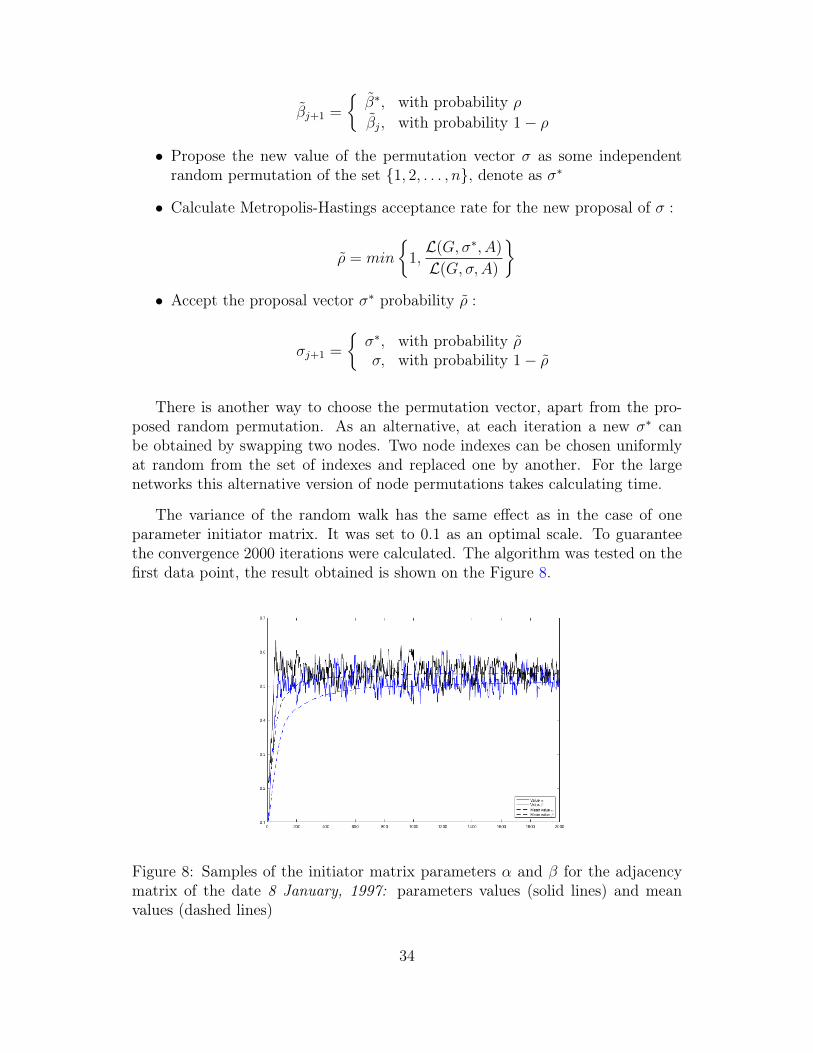
The variance of the random walk has the same effect as in the case of oneparameter initiator matrix. It was set to 0.1 as an optimal scale. To guaranteethe convergence 2000 iterations were calculated. The algorithm was tested on thefirst data point, the result obtained is shown on the Figure 8.

Figure 8: Samples of the initiator matrix parameters α and β for the adjacencymatrix of the date 8 January, 1997: parameters values (solid lines) and meanvalues (dashed lines)

34

It is interesting to see that estimated values for both parameters α and β areclose to the value of the previously estimated parameter p for the correspondingadjacency matrix, that is around 0.5. Though the estimation values are similar,the interpretation for these two models is distinctive. The form of the 2 parameterKronecker graph is no longer identical entries, as in the previous model. Elementsof the Kronecker graph G = Θ(α, β)[k] are interpreted as the probabilities, thoughtheir numerical values are different from the initial parameters α and β.

Figure 9: Kernel density estimation for the values of Kronecker graphG = Θ(α, β)[k]

Figure 10: Kernel density estimation for the values of Kronecker graphG = Θ(α, β)[k], linear rescaling

The computed values are too small to be considered as a realistic probabilitiesof edges. Their distribution can serve as a approximate shape of the graph.

35

7 Conclusion

The implementation of the Markov Chain Monte Carlo sampling method for theparameters of random graph and Kronecker graph models provided useful resultsfor fitting the model to the real world data. These results can be explained bythe empirical events of financial crisis.

The parameter of the random graph p that serves as an estimated measure ofconnectedness among nodes demonstrates high values during the times of financialinstability, that goes in line with the existing results of financial networks studies.The estimated parameters of the Kronecker graph model provide an abstracttopological structure of the observed network. The shape of the parameters’distribution confirms imbalanced structure in the connectivity level of nodes thatcan be interpreted as a community structure of the financial system.

36

References

[Acemoglu et al., 2013] Acemoglu, D., Ozdaglar, A., and Tahbaz-Salehi, A.(2013). Systemic risk and stability in financial networks. Working Paper 18727,National Bureau of Economic Research.

[Aicher et al., 2014] Aicher, C., Jacobs, A. Z., and Clauset, A. (2014). Learninglatent block structure in weighted networks. Journal of Complex Networks,3(2):221–248.

[Albert and Barabási, 2002] Albert, R. and Barabási, A.-L. (2002). Statisticalmechanics of complex networks. Reviews of modern physics, 74(1):47.

[Barabási, 2009] Barabási, A.-L. (2009). Scale-free networks: a decade and be-yond. Science, 325(5939):412–413.

[Barabási and Albert, 1999] Barabási, A.-L. and Albert, R. (1999). Emergence ofscaling in random networks. Science, 286(5439):509–512.

[Billio et al., 2016] Billio, M., Casarin, R., Costola, M., and Pasqualini, A. (2016).An entropy-based early warning indicator for systemic risk. Journal of Inter-national Financial Markets, Institutions and Money, 45:42–59.

[Billio et al., 2010] Billio, M., Getmansky, M., Lo, A. W., and Pelizzon, L. (2010).Econometric measures of systemic risk in the finance and insurance sectors.Working Paper 16223, National Bureau of Economic Research.

[Billio et al., 2012] Billio, M., Getmansky, M., Lo, A. W., and Pelizzon, L. (2012).Econometric measures of connectedness and systemic risk in the finance andinsurance sectors. Journal of Financial Economics, 104(3):535–559.

[Bollobás, 2013] Bollobás, B. (2013). Modern graph theory, volume 184. SpringerScience & Business Media.

[Casarin et al., 2017] Casarin, R., Costola, M., and Yenerdag, E. (2017). Finan-cial bridges and network communities.

[Diestel, 2000] Diestel, R. (2000). Graph theory Springer-Verlag Berlin and Hei-delberg GmbH & amp.

[Elliott et al., 2014] Elliott, M., Golub, B., and Jackson, M. O. (2014). Financialnetworks and contagion. American Economic Review, 104(10):3115–53.

[Erdös and Rényi, 1959] Erdös, P. and Rényi, A. (1959). On random graphs, i.Publicationes Mathematicae (Debrecen), 6:290–297.

[Hastings, 1970] Hastings, W. K. (1970). Monte carlo sampling methods usingmarkov chains and their applications. Biometrika, 57(1):97–109.

37

[Holland et al., 1983] Holland, P. W., Laskey, K. B., and Leinhardt, S. (1983).Stochastic blockmodels: First steps. Social networks, 5(2):109–137.

[Hurd, 2016] Hurd, T. R. (2016). Contagion! Systemic Risk in Financial Net-works. Springer.

[Lancaster, 2004] Lancaster, T. (2004). An introduction to modern Bayesianeconometrics. Blackwell Oxford.

[Leskovec et al., 2005a] Leskovec, J., Chakrabarti, D., Kleinberg, J., and Falout-sos, C. (2005a). Realistic, mathematically tractable graph generation and evo-lution, using kronecker multiplication. In European Conference on Principlesof Data Mining and Knowledge Discovery, pages 133–145. Springer.

[Leskovec et al., 2010] Leskovec, J., Chakrabarti, D., Kleinberg, J., Faloutsos, C.,and Ghahramani, Z. (2010). Kronecker graphs: An approach to modeling net-works. Journal of Machine Learning Research, 11(Feb):985–1042.

[Leskovec et al., 2005b] Leskovec, J., Kleinberg, J., and Faloutsos, C. (2005b).Graphs over time: densification laws, shrinking diameters and possible expla-nations. In Proceedings of the eleventh ACM SIGKDD international conferenceon Knowledge discovery in data mining, pages 177–187. ACM.

[Metropolis et al., 1953] Metropolis, N., Rosenbluth, A. W., Rosenbluth, M. N.,Teller, A. H., and Teller, E. (1953). Equation of state calculations by fastcomputing machines. The journal of Chemical Physics, 21(6):1087–1092.

[Robert and Casella, 2011] Robert, C. and Casella, G. (2011). A short historyof markov chain monte carlo: Subjective recollections from incomplete data.Statistical Science, pages 102–115.

[Slovik, 2012] Slovik, P. (2012). Systemically important banks and capital reg-ulation challenges. OECD Economics Department Working Papers, No. 916,OECD Publishing

[Watts and Strogatz, 1998] Watts, D. J. and Strogatz, S. H. (1998). Collectivedynamics of ‘small-world’networks. nature, 393(6684):440.

[Weichsel, 1962] Weichsel, P. M. (1962). The kronecker product of graphs. Pro-ceedings of the American mathematical society, 13(1):47–52.

38