Master Thesis Draft - Unit
119
Transcript of Master Thesis Draft - Unit


i
Abstract
The objective of this master thesis is to quantify how the estimated uncertainty, associated
with the Hyme field, will change as more data becomes available. This will be done by
identifying the key uncertainties and comparing the pre/post -production estimated ultimate
oil recovery and hence the long term potential of Hyme. Hyme is classified as a fast-track
development, which means that limited technical subsurface work has been performed
before the production start-up. There are limited data available, and no cores where taken.
The objective was achieved through a process that involved three major tasks. The first task
was to adjust geologic and reservoir simulation models to establish a working reservoir
simulation model and to generate a model reference case to be used in the uncertainty
analysis. Secondly, a stochastic pre-production uncertainty analysis was performed in order
to quantify the range of ultimate estimated oil recovery and the governing parameters that
affect this. The final task was to perform a post-production uncertainty analysis, which
utilizes actual bottom hole pressure data with a computer assisted history matching process.
The study concludes that the uncertainty associated with the Hyme subsurface was reduced
with early data. Based on the results of the pre-production uncertainty analysis, the ultimate
estimated oil recovery can be described within the range of 3.40 to 5.44 million Sm3. The
post-production uncertainty analysis resulted in a range of 4.01 to 5.21 million Sm3. Hence
the uncertainty range for the ultimate estimated oil recovery and the risk concerning the
long term potential of Hyme was reduced.

ii
Acknowledgements
This report presents the results of a master thesis by Mats Betanzo Bratteli at the
Department of Petroleum Engineering, University of Stavanger. The work has been
performed from December 2012 through June 2013.
This thesis would not have been possible without the support of many people. Firstly, I wish
to express my gratitude to my main supervisor, Sjur Arneson (Director Reservoir Evaluation,
VNG Norge AS) who offered invaluable assistance, support and guidance. I would also like to
express my very appreciation to my faculty supervisor Svein M. Skjæveland (Professor of
petroleum engineering, University of Stavanger) for his expert advises and suggestions
during this thesis work.
I am particularly grateful for the assistance given by Kevin Best (Reservoir Engineering
Advisor, VNG Norge AS), for the great conversations, suggestions and technical support. A
deep thank to Adrian Anton (Reservoir Engineer, Schlumberger) for hosting a great course in
Petrel, and for continuous technical support. I would also like to thank Karl Ludvig Heskestad
(Commercial Director, Resoptima) for a personal training course in Olyx, and for technical
support during this study.
Special thanks to Andre Sætheren (Senior Reservoir Engineer, VNG Norge AS), Ali Jaffri
(Geological Consultant, Applied Stratigraphix), and Margaret Åsly (Senior Reservoir Engineer,
VNG Norge AS) for advises and inputs during this study.
I would like to express my profound gratitude and appreciation to VNG Norge AS for support
and participation in this study. To be a part of the Hyme asset and to be allowed to
contribute with subsurface technical work has been a great motivator during the study. I will
also like to thank the companies Statoil ASA, E.ON Ruhrgas Norge AS, GDF Suez E&P Norge
AS, Core Energy and Faroe Petroleum for permission to use the necessary data.
Finally, I wish to thank my common law wife for support, patience and encouragement
throughout my study.
Stavanger 13th of June 2013
……………………………………..
Mats Betanzo Bratteli

iii
Table of Contents Abstract ................................................................................................................................................ i
Acknowledgements ..............................................................................................................................ii
List of figures ....................................................................................................................................... vi
List of tables ........................................................................................................................................ ix
1. Introduction ......................................................................................................................................... 1
2. Background .......................................................................................................................................... 3
3. Model Reference Case ......................................................................................................................... 6
3.0.1 Reservoir Simulation .............................................................................................................. 6
3.0.2 Workflow for development of Hyme reference case ........................................................... 10
3.1 Reservoir and model description ................................................................................................ 11
3.2 Hyme static data .......................................................................................................................... 12
3.2.1 Rock properties .................................................................................................................... 12
3.2.2 Fluid properties .................................................................................................................... 16
3.3 Hyme dynamic data ..................................................................................................................... 18
3.3.1 Faults .................................................................................................................................... 18
3.3.3 Vertical communication ....................................................................................................... 18
3.3.4 Permeability ......................................................................................................................... 20
3.3.5 Relative permeability............................................................................................................ 20
3.3.6 Capillary pressure ................................................................................................................. 26
3.4 Hyme simulation model .............................................................................................................. 27
3.4.1 Simulation Grid ..................................................................................................................... 27
3.4.2 In-Place volumes................................................................................................................... 27
3.4.3 Wells ..................................................................................................................................... 28
3.5 Development Strategy ................................................................................................................. 29
3.6 Hyme Reference case Results ...................................................................................................... 30
4. Pre-production Uncertainty Study .................................................................................................... 34
4.0.1 Stochastic modeling ............................................................................................................. 34
4.0.2 Monte Carlo sampling .......................................................................................................... 35
4.0.2 Workflow for Pre-production uncertainty study .................................................................. 36
4.1 Uncertainty Parameters .............................................................................................................. 37
iv
4.1.1 In-Place volumes................................................................................................................... 37
4.1.2 Permeability ......................................................................................................................... 38
4.1.3 Relative permeability............................................................................................................ 38
4.1.4 Fault Seal .............................................................................................................................. 41
4.1.5 Vertical communication ....................................................................................................... 42
4.1.6 Summary of input parameters to uncertainty study ............................................................ 42
4.2 Pre-production uncertainty study results ................................................................................... 44
4.3 Sensitivities .................................................................................................................................. 44
4.3.1 Sensitivities for oil volumes in-place .................................................................................... 44
4.3.2 Sensitivities for cumulative oil production ........................................................................... 45
4.4 Pre-production uncertainty simulation Results .......................................................................... 52
4.4.1 Production (Oil, gas, and water) ........................................................................................... 53
4.4.2 Injection (Water) .................................................................................................................. 56
4.4.3 Discussion concerning pre-production simulation results ................................................... 57
4.5 Pre-production estimated ultimate oil recovery ......................................................................... 58
5. Post-production Uncertainty Study ................................................................................................... 61
5.0.1 History Matching .................................................................................................................. 61
5.0.2 Objective function ................................................................................................................ 62
5.0.3 Integration of history matching in uncertainty study .......................................................... 63
5.0.4 Workflow for Post-production uncertainty study ................................................................ 65
5.1 Bottom hole pressure data .......................................................................................................... 66
5.1.1 Determination of objective value criteria for history matching........................................... 67
5.2 Post-production uncertainty analysis results .............................................................................. 68
5.3 Post-production uncertainty input parameters .......................................................................... 68
5.4 Post-production simulation results ............................................................................................. 69
5.4.1 Production (Oil, gas, and water) ........................................................................................... 70
5.4.2 Injection (Water) .................................................................................................................. 73
5.5 Post-production estimated ultimate oil recovery ....................................................................... 74
6. Pre/post-production uncertainty discussion ..................................................................................... 77
7. Conclusions ........................................................................................................................................ 81

v
8. References ......................................................................................................................................... 82
9. Appendix A ........................................................................................................................................ 84
Hyme Reference case: – Eclipse 100 simulation deck ....................................................................... 84
'MB_REFERENCE_PROPS.INC' / ..................................................................................................... 88
'MB_REFERENCE_SCH.INC' / ....................................................................................................... 102

vi
List of figures
Figure 2-1: Location of the Hyme field on the Norwegian continental shelf............................. 3
Figure 2-2: Geologic depth map of the Hyme reservoir. ........................................................... 5
Figure 3-1: Schematic overview of the workflow for developing Hyme reference case. ........ 10
Figure 3-2: 2D overview of the initial saturations on the Hyme field. ..................................... 16
Figure 3-3: 3D cross section of the initial saturations on the Hyme field. ............................... 17
Figure 3-4: Vertical cross section of the 3D Grid displaying the different reservoir zones,
location of transmissibility multipliers (Z1, Z2, Z3, Z4), the two segments and the internal
fault G2. .................................................................................................................................... 19
Figure 3-5: Oil-Water relative permeability for SATNUM 1 ..................................................... 24
Figure 3-6: Gas-Oil relative permeability for SATNUM 1 ......................................................... 24
Figure 3-7: Oil-Water relative permeability for SATNUM 2. .................................................... 25
Figure 3-8: Gas-Oil relative permeability for SATNUM 2. ........................................................ 25
Figure 3-9: Oil-Water capillary pressure curve for both SATNUM 1 and SATNUM 2. ............. 26
Figure 3-10: 3D grid of western and eastern segments with well locations and the internal
fault (G2) dividing the reservoir into the two parts. ................................................................ 28
Figure 3-11: Predicted oil rate and cumulative oil production for Hyme reference case. ...... 31
Figure 3-12: Predicted gas rate and cumulative gas production for Hyme reference case. ... 31
Figure 3-13: Predicted water rate and cumulative water production for Hyme reference case.
.................................................................................................................................................. 32
Figure 3-14: Predicted water injection rate and cumulative water injection for Hyme
reference case. ......................................................................................................................... 32
Figure 3-15: Predicted reservoir pressure, gas-oil ratio and water cut for Hyme reference
case. .......................................................................................................................................... 33
Figure 4-1: Schematic overview of pre-production uncertainty study. ................................... 36
Figure 4-2: Oil-Water relative permeability for SATNUM 1 displaying base, low and high
cases. ........................................................................................................................................ 39
Figure 4-3: Gas-Oil relative permeability for SATNUM 1 displaying base, low and high cases.
.................................................................................................................................................. 40
Figure 4-4: Oil-Water relative permeability for SATNUM 2 displaying base, low and high cases
.................................................................................................................................................. 40
vii
Figure 4-5: Gas-Oil relative permeability for SATNUM 2 displaying base, low and high cases.
.................................................................................................................................................. 41
Figure 4-6: Tornado plot of difference in oil volume in-place between sensitivities and the
Hyme reference case. ............................................................................................................... 45
Figure 4-7: Tornado plot of difference in cumulative oil production between sensitivities and
the Hyme reference case at 01.01.2018. ................................................................................. 48
Figure 4-8: Tornado plot of difference in cumulative oil production between sensitivities and
the Hyme reference case at 01.01.2020. ................................................................................. 48
Figure 4-9: Tornado plot of difference in cumulative oil production between sensitivities and
the Hyme reference case at 01.01.2025. ................................................................................. 49
Figure 4-10: Tornado plot of difference in umulative oil production between sensitivities and
the Hyme reference case at 01.01.2030. ................................................................................. 49
Figure 4-11: Oil production rates from pre-production uncertainty simulations.................... 53
Figure 4-12: Cumulative oil production from pre-production uncertainty simulations. ......... 53
Figure 4-13: Gas production rates from pre-production uncertainty simulations .................. 54
Figure 4-14: Cumulative gas production from pre-production uncertainty simulations. ....... 54
Figure 4-15: Water production rates from pre-production uncertainty simulations .............. 55
Figure 4-16: Cumulative water production from pre-production uncertainty simulations. ... 55
Figure 4-17: Water injection rates from pre-production uncertainty simulations .................. 56
Figure 4-18: Cumulative water injection from pre-production uncertainty simulations. ....... 56
Figure 4-19: Distribution of cumulative oil production based on pre-production simulation
results. ...................................................................................................................................... 59
Figure 4-20: Pre-Production histogram distribution of estimated ultimate oil recovery. ....... 59
Figure 4-21: Pre-Production histogram versus cumulative distribution function ................... 60
Figure 5-1: Workflow for Post-production uncertainty study ................................................. 65
Figure 5-2: Measured bottom hole pressure compared with Hyme reference case where day
0 is April 2 2013. ....................................................................................................................... 67
Figure 5-3: Oil production rates from post-production simulations........................................ 70
Figure 5-4: Cumulative oil production from post-production simulations. ............................. 70
Figure 5-5: Gas production rates from post-production simulations ...................................... 71
Figure 5-6: Cumulative gas production from post-production simulations. ........................... 71
Figure 5-7: Water production rates from post-production simulations .................................. 72
viii
Figure 5-8: Cumulative water production from post-production simulations. ....................... 72
Figure 5-9: Water injection rates from post-production simulations ...................................... 73
Figure 5-10: Cumulative water injection from post-production simulations. ......................... 73
Figure 5-11: Distribution of cumulative oil production based on post-production simulation
results ....................................................................................................................................... 75
Figure 5-12: Post-Production histogram distribution of estimated ultimate oil recovery ...... 75
Figure 5-13: Post-Production histogram versus cumulative distribution function.................. 76
Figure 6-1: Pre/post-comparison of distribution of cumulative oil production. ..................... 79
Figure 6-2: pre/post-production estimated ultimate oil recovery uncertainty ranges ........... 80

ix
List of tables
Table 3-1: Average true vertical thickness by reservoir zone. ................................................. 12
Table 3-2: Rock compressibility ................................................................................................ 12
Table 3-3: Average Porosity, Shale volume fraction, and net to gross by reservoir zone. ...... 14
Table 3-4: Average water saturation by reservoir zone. .......................................................... 15
Table 3-5: Average Oil water contact for the Tilje formation. ................................................. 16
Table 3-6: PVT data from Tilje formation. ................................................................................ 17
Table 3-7: Transmissibility multipliers between the different reservoir zones. ...................... 19
Table 3-8: Average horizontal and vertical permeability for the different reservoir zones. ... 20
Table 3-9: Relative permeability input for the Hyme reference case. ..................................... 22
Table 3-10 Constant endpoint properties for relative permeability ........................................ 23
Table 3-11: Grid dimensions for the Hyme reference case. .................................................... 27
Table 3-12: In-place volumes for Hyme reference case ........................................................... 27
Table 3-13: Well and production constraints ........................................................................... 29
Table 3-14: Cumulative production results for Hyme reference case. .................................... 30
Table 4-1: Uncertainty ranges for pore volume multipliers for eastern and western segment.
.................................................................................................................................................. 37
Table 4-2: Uncertainty ranges for pore volume in eastern and western segment.................. 37
Table 4-3: Uncertainty ranges for horizontal and vertical permeability in the Tilje formation.
.................................................................................................................................................. 38
Table 4-4: Uncertainty ranges for horizontal and vertical permeability multipliers in the Tilje
formation. ................................................................................................................................. 38
Table 4-5: Uncertainty input data for relative permeability. ................................................... 39
Table 4-6: Relative permeability discrete input parameters for uncertainty study. ............... 41
Table 4-7: Fault seal discrete input parameters for uncertainty study. .................................. 42
Table 4-8: Uncertainty ranges for transmissibility multipliers between the different reservoir
zones. ........................................................................................................................................ 42
Table 4-9: Summary of input parameters to uncertainty study. ............................................. 43
Table 4-10: Oil volumes in-place by sensitivities. .................................................................... 44
Table 4-11: Cumulative oil production by sensitivities at 01.01.2018. .................................... 46
Table 4-12: Cumulative oil production by sensitivities at 01.01.2020. .................................... 46
Table 4-13: Cumulative oil production by sensitivities at 01.01.2025. .................................... 47
x
Table 4-14: Cumulative oil production by sensitivities at 01.01.2030. .................................... 47
Table 4-15: Distribution of cumulative oil production based on pre-production simulation
results. ...................................................................................................................................... 58
Table 5-1: Bottom hole pressure from Hyme in the period 02.03-24.04 2013 ....................... 66
Table 5-2: Ranges for post-production uncertainty input parameters .................................... 68
Table 5-3: Distribution of cumulative oil production based on post-production simulation
results ....................................................................................................................................... 74
Table 6-1: Comparison of pre/post-production low case input parameters ........................... 77
Table 6-2: Comparison of pre/post-production high case input parameters .......................... 78
1
1. Introduction
The objective of this thesis is to describe and quantify static and dynamic uncertainty
associated with the development of a new oil field named Hyme. In order to describe and
quantify these uncertainties, existing tools and techniques are used in combination with
available geophysical, geologic, petrophysical, reservoir, drilling, and production data. The
study focuses on an uncertainty analysis both before and after production start-up of the
field. The overall purpose of this thesis is to quantify how perceived uncertainty will change
as more data becomes available. This will be done by comparing the estimated ultimate oil
recovery before and after the field starts production. To reach the main objective, technical
work was divided into 3 main tasks.
The first task was to adjust the geologic and reservoir simulation models provided by the
operator to establish a working reservoir simulation model and to generate a model
reference case to be used in the uncertainty analysis. A description of the different input
parameters, how the reference case is established and the results of the reference case, are
described in chapter 3.
The second task was to perform a stochastic pre-production uncertainty analysis in order to
quantify the range of ultimate estimated oil recovery and the governing parameters that
affect this. A sensitivity analysis was performed of selected input parameters and 200
simulations were run for investigating the estimated ultimate oil recovery. In chapter 4 the
uncertainty ranges for the input parameters are described as well the methodology and
results of this task.
The final task was to integrate production data into the uncertainty study, in order to
perform a post-production uncertainty analysis. This is known as history matching, and it will
integrate actual production data into the simulator. In this thesis the history matching will be
performed with assisted history matching software (Olyx). The aim of history matching is to
provide a more representative model. Methodology and results for this study are described
and presented in chapter 5.
Mapping of uncertainty associated with field development in the petroleum industry has
become more important over the years, as the costs for developing a field and to collect the
2
necessary data is becoming increasingly expensive. There are several available uncertainty
studies that have been performed with simulations to predict future performance of a
reservoir behavior (Walstrom et al., 1967), (Damsleth et al., 1992), (Steagall and Schozer,
2001), (Li-Bong et al,. 2006) and (Lisboa and Duarte, 2010).
Walstrom et al. (1967) presented a method that incorporates uncertainty in the input
parameters to a reservoir simulation model. Uncertainty was included in that more
simulation models were run with different input parameters to compare the results
statistically. A more efficient approach was proposed by Damsleth et al. (1992), where a
methodology with experimental design was presented. Experimental design can be
considered as a plan that specifies the setting of each input parameter in a series of
simulation runs.
Steagall and Schozer (2001) presented a methodology of defining a set of uncertain
parameters, performing a sensitivity analysis of the parameters, and then generating a
number of simulation cases with experimental design. After the simulations were done, the
results were treated statistically. The study was performed on the appraisal stage applied to
a real offshore field in Campos Basin in Brazil. A model based uncertainty analysis
methodology presented by Li-Bong et al (2006) uses a similar methodology, however this
model based methodology incorporates multiple geologic models as well. These
methodologies are analogues and form the basis of the methodology used in this thesis.
Lisboa and Duarte (2010) present a study incorporating history matching with the
uncertainty study. The study is performed on a deep water oil field in the Campos Basin,
where the field has been in production for a few years.
This thesis adopts a mix of the methods mentioned above, but differ in the extent that it
concerns a new oil field in the initial production phase, where uncertainty is assessed both
before and after production start-up. In addition to this, the experimental design could be
considered as unique when it comes to which input parameters that are integrated at the
same time and the software used for history matching.
3
2. Background
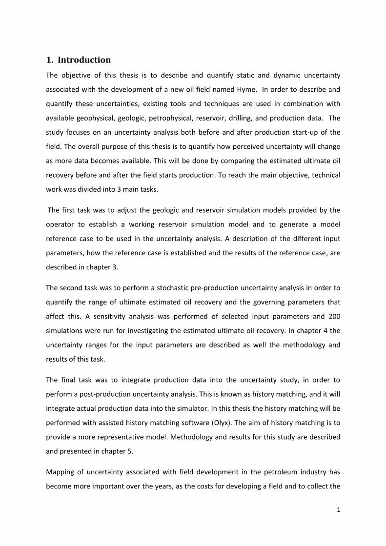
The Hyme field is an oil field located in the Haltenbanken area (block 6407/8) on the
Norwegian continental shelf northwest of Trondheim (Figure 2-1). The field is located
offshore in water depth of 250m. It was discovered in May of 2009 with the exploration well
6407/8-5 S and its sidetrack 6407/8-5 A. Hyme is described as a fast track development
which implies a rapid design, construction, and installation. Additionally, Hyme will be a tie
in to the already producing field Njord. This means that production is to the Njord A
platform, through a 19 km long pipeline south-east of Hyme. Production started on the 2nd
of March 2013, and the field is operated by Statoil, which owns 20% of the license. Other
companies that are partners in the development are E.ON Ruhrgas Norge AS (30%), GDF
Suez E&P Norge AS (28%), Core Energy (12%), Faroe Petroleum (7.5%) and VNG Norge AS
(2.5%).
Hyme has a limited volume of data available. Two seismic surveys with poor to moderate
quality define the structure while well logs are used to describe the internal architecture of
reservoirs. Cores were not extracted from the field, which means that analogue data from
Figure 2-1: Location of the Hyme field on the Norwegian continental shelf.
4
nearby fields such as Njord and Heidrun which have similar geology will be used.
Hydrocarbons were discovered both in Tilje and Ile formations, however more than 90% of
the reserves are estimated to be located in Tilje. The field development is only focused on
the Tilje reservoir.
The primary reservoir in the Hyme Field is the Lower Jurassic Tilje Formation (Dalland et al,
1988). The Tilje represents ancient tide-dominated delta sediments that were deposited in a
rift-basin (Martinius et al ., 1999). Due to the complex interplay between river, tide, and to a
lesser extent, wave processes, tidal deltas tend to produce extremely heterogeneous
successions. Sands occur in tidal sand flats, channels, shore-normal tidal mouthbars, and
subtidal dunes. The majority of these sand-prone lithofacies have internal mud-drapes.
These mud-drapes can reach thickness of 1 cm and decrease vertical permeability. Studies
performed on Tilje, based on pressure data from Heidrun, have identified these barriers
(Reid et al.,1996). It is likely that these barriers also exist in Tilje formation of Hyme, making
it one of the key uncertainties in this study. Besides internal flow barriers, another major
uncertainty lies with the laterally discontinuous nature of sand bodies. Channels in tidal
deltas have a low tendency to avulse, which means they do not meander freely, and do not
produce sheet-like sand bodies. Tidal bars also form isolated sand bodies that are not
connected. Therefore a borehole that intersects one of these compartmentalized sand-
bodies may only drain that one particular unit.
There is one oil production well on Hyme and it is a multilateral with two branches. The main
reason for the multilateral well is that the Hyme reservoir has a major fault dividing the
reservoir into two parts, in eastern and western segment. The main bore is located in the
largest segment, which is west, while the lateral bore is located in east. The eastern segment
is smaller; therefore water breakthrough is predicted to come earlier in the lateral bore,
compared to the main bore. This would result in a possible earlier shut in for this lateral and
the model predicts this to occur in 2016.
To provide pressure support to the multilateral producer a water injector is planned. The
injector is located in the northern part of the eastern segment, where the major fault has
the smallest throw (Figure 2-2). Location of the injector was carefully decided by the license
group based on a cross-disciplinary evaluation, including structural uncertainties. The
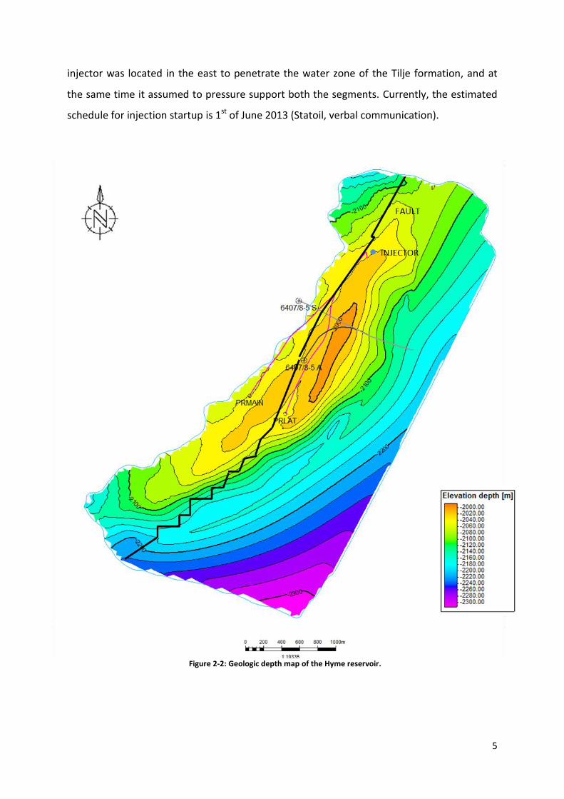
5
injector was located in the east to penetrate the water zone of the Tilje formation, and at
the same time it assumed to pressure support both the segments. Currently, the estimated
schedule for injection startup is 1st of June 2013 (Statoil, verbal communication).
Figure 2-2: Geologic depth map of the Hyme reservoir.
6
3. Model Reference Case
Geologic and simulation models were provided by the operator Statoil. The models consist
of static and dynamic input data, which is based on geologic, geophysical, petrophysical,
reservoir engineering, production and drilling data. The first task was to create a reference
case for prediction of future production performance of the Hyme reservoir (Figure 3-1).
Based on these results, an uncertainty study was performed to investigate which parameters
affect the initial in-place oil volume and the cumulative oil production.
3.0.1 Reservoir Simulation
Reservoir simulation is one of the most flexible and used tools in reservoir engineering. This
is mainly because it is a tool that has the ability to predict the future production
performance of oil and gas reservoirs over a wide range of operating conditions (Mattax and
Dalton, 1990). To run a simulation model, it is necessary to have a model that represents the
reservoir of interest. The model should contain information about the rock and fluid
properties obtained by laboratory measurements of cores, well logs and seismic. All this
information combined with interpretation of the results are called physical models (Kleppe,
2010). The input data for the Hyme reference case was provided by Statoil and are described
in the reservoir and model description (section 3.1) of this thesis.
To be able to run a simulation on a physical reservoir model the model needs to be divided
into a number of individual blocks, known as grid blocks. These blocks correspond to a
unique location in the reservoir, with unique properties such as porosity, permeability and
relative permeability that will represent the reservoir at this location. In a 3D grid, which will
be used for the Hyme reference case, the grid blocks are assigned x, y and z coordinates
(Mattax and Dalton, 1990).
A reservoir simulator can be defined as a computer program written to solve the equations
for flow of fluids in a reservoir (Kleppe, 2010). During simulation, fluids can flow between
neighboring grid blocks. The rate of this flow is determined by pressure differences between
blocks and flow properties assigned to the interfaces between the blocks. This process will
minimize the mathematical problem to a calculation of flow between grid blocks. For every
interface between different grid blocks, a set of equations must be solved in order to
calculate the flow of all mobile phases. In general, the equations include Darcy’s law and the

7
concept of material balance and contain terms describing the permeability between grid
blocks, fluid mobilities including relative permeability and viscosity, and compressibility of
the rock and fluids (Mattax and Dalton, 1990).
There are several types of reservoir simulators, depending on which reservoir they are
intending to simulate. For the Hyme reference case, a black oil model will be used. The
simulator is Eclipse 100, developed by Schlumberger. Black oil model simulators are the
most frequently used simulators in the petroleum industry, because it is the simplest model.
The reason why it is considered as simple is the assumptions for the black oil model which
are:
- Three phases, oil, gas and water.
- Three components; oil, gas and water.
- No phase transfer between water and hydrocarbons.
- Gas can be dissolved in oil and flow together with oil component in an oil phase.
- Oil cannot exist in the gas phase.
- Constant temperature.
Based on these assumptions, the black oil model consists of two hydrocarbon components.
This is assumed to be appropriate for Hyme reference case, since changes in fluid
compositions are not believed to play an integral part of the process. The three components
are given the same names as the phases. That will not cause any problems for the water
phase, since it is assumed to be no phase transfers between water and hydrocarbons.
Between the oil and gas component there is a more complex relation since there is a one
way transition. This means that it can exists gas in the oil phase, but not oil in the gas phase.
Since Hyme is not a gas condensate field, these assumptions are expected to be valid.
Additionally, the temperature is always assumed to be constant (Kleppe, 2010).
The final equations for the black oil model are based on differential equations for mass
conservation for each component combined with Darcy’s law. They are given by
water
*[ ]
( )+
( )

8
oil
*[ ]
( )+
( )
and gas
*[ ]
( )+ *
[ ]
( )+
(
)
where:
Index o, w, c: oil, water and gas.
Q: Source/sink term, positive for injection, negative for production
S: Saturation
B: Formation volume factor
Rs: Gas Solubility
Kr: Relative permeability
[K]: Absolute permeability
P: Pressure
: g
: Phase density
: Gravity acceleration
: Distance
: Porosity
Before a reservoir simulator can run and predict future production performance, one must
create a development strategy. This includes wells, production schedule and constraints.
Number of producing and injecting wells must be specified, and under which conditions they
can operate. Several wells can have group constraints, which can be flow rate or pressure
related. The constraints can be economic limits or what the production facility actually can
handle. The production schedule must also be specified, when production starts and for how
long the run will last (Mattax and Dalton, 1990),(Kleppe, 2010). Development strategy for
Hyme reference case was carefully created based on well and facility constraints provided by

9
Statoil. This will be further discussed in the development strategy section (section 3.5) of this
thesis.
A standard procedure after the reservoir model is constructed is to test it against historical
production data. The aim is to investigate if it is possible to duplicate past field behavior,
running a simulator with historical data and compare the calculated production behavior
with actual reservoir performance (Breitenbach, 1991), known as history matching. The
Hyme reference case is a new development based on no production or pressure data, thus
history matching was not considered. However, for the post uncertainty study, history
matching will be applied.
Computer software (Petrel) was used for modeling, visualization, and post-processing. Petrel
is a PC-based workflow application for subsurface interpretation, integration, and modeling.
The software makes it possible for users to perform different workflows, from seismic
interpretation to reservoir simulation. A benefit using this software is that geophysicists,
geologists, and reservoir engineers can move across domains, rather than applications,
through the Petrel integrated toolkit. Petrel is developed by Schlumberger, and uses the
simulator Eclipse 100. (Schlumberger, 2012)
10
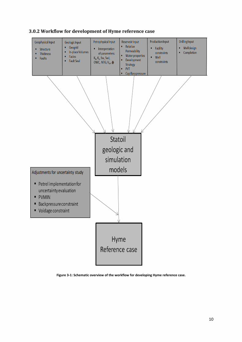
3.0.2 Workflow for development of Hyme reference case
Figure 3-1: Schematic overview of the workflow for developing Hyme reference case.

11
3.1 Reservoir and model description
The input parameters used in this thesis, are based on Statoils early evaluation of the Hyme
field. A geophysical study was performed by Statoil to generate a structural model for the
Hyme reservoir. The structural model is based on seismic interpretations and it also includes
location of the internal fault. From the seismic interpretations, the reservoir thickness was
determined.
A geological evaluation of the Hyme field was performed by Statoil. The study has been
simplified to meet the deadlines of the fast track work plan. The consequence is that
parameters were modeled directly, without facies modeling. Another time saving decision
was to build a geogrid that allows simulation without upscaling. The purpose for the
geological evaluation has been to quantify the in-place volumes for the Tilje reservoir of the
Hyme structure, create a grid for simulation, and quantify the uncertainties on in-place
volumes. In addition a fault seal study was performed for investigating flow through the
internal fault (Statoil, 2012).
A Petrophysical study was performed by Statoil to determine porosity, shale volume, oil-
water contact, net sand, permeability, water saturation and a J function. The interpretation
was based on the total porosity model using data from well logs and data from analogue
fields in the area. The formation of interest in this study was Tilje (Statoil, 2012).
Reservoir data includes relative permeability, PVT and capillary pressure. Statoil performed
an analogue study in order to obtain relative permeability and capillary pressure data. The
PVT data were based on fluid lab analysis of samples from well 6407/8-5S and 6407/8-5A
supplied by Statoil (Statoil, 2012).
In this thesis, the different input parameters are divided into two groups, static and dynamic
input parameters. Static parameters include parameters that have an impact on volumes in
place. Dynamic parameters include parameters that influence the flow of hydrocarbons and
water and influences cumulative oil recovery.
12
3.2 Hyme static data
3.2.1 Rock properties
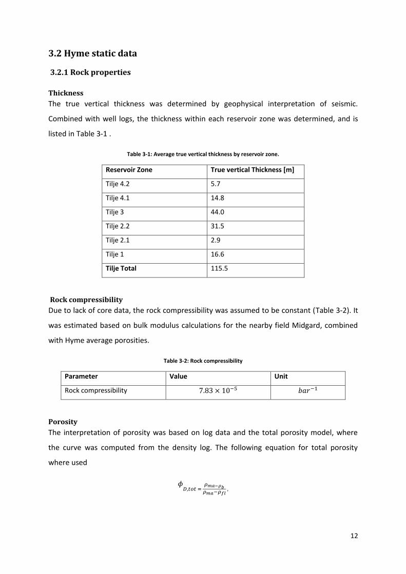
Thickness
The true vertical thickness was determined by geophysical interpretation of seismic.
Combined with well logs, the thickness within each reservoir zone was determined, and is
listed in Table 3-1 .
Table 3-1: Average true vertical thickness by reservoir zone.
Reservoir Zone True vertical Thickness [m]
Tilje 4.2 5.7
Tilje 4.1 14.8
Tilje 3 44.0
Tilje 2.2 31.5
Tilje 2.1 2.9
Tilje 1 16.6
Tilje Total 115.5
Rock compressibility
Due to lack of core data, the rock compressibility was assumed to be constant (Table 3-2). It
was estimated based on bulk modulus calculations for the nearby field Midgard, combined
with Hyme average porosities.
Table 3-2: Rock compressibility
Parameter Value Unit
Rock compressibility
Porosity
The interpretation of porosity was based on log data and the total porosity model, where
the curve was computed from the density log. The following equation for total porosity
where used
13
where ϕD,tot is the total porosity, ρma is the matrix density, ρb is the bulk density from logs
and ρfl is the fluid density. Due to lack of core data on Hyme, the matrix density coming from
core data from the relevant formation units from wells in the area, and then averaged over
each formation.
Base case porosity function PHIT, is taken from the average porosity of Tilje in both wells.
Since the locations of the two wells are close, it is assumed that the reservoir quality is
similar. However, the TVD depth is deeper in the S well compared to well A, which could
result in lower porosity. Results for porosity in the different reservoir zones are listed in Table
3-3.
Shale volume
The calculation of shale volume fraction was based on a minimum of two estimates. The first
estimate from gamma-ray log and the second estimate from neutron porosity log data. The
shale volume equation is given by
( ),
with the volume shale fraction from gamma-ray given by
where γ is the read of the gamma-ray log, γmax is the shale gamma-ray value, and γmin is the
clean sand gamma-ray value (Lehne, 1985).
The volume shale fraction from density neutron is given by
where ϕNc is the borehole corrected neutron porosity from log converted to sandstone
porosity units, ϕD,tot is the total porosity form the density log and ϕNsh is the apparent shale
neutron porosity from literature (Lehne, 1985). The Hf is the fluid hydrogen index. Shale
volume fractions for the different reservoir zones are listed in Table 3-3.

14
Net sand
Since no core data were available, the Net sand cut-offs was defined to minimize loss of
hydrocarbon volume, and at the same time estimate volumes that are clearly non net from
logs. Statoil proposed a porosity cut-off of 14% and a shale volume fraction cut-off of 0.35%.
The proposed cut-offs are reported to result in a loss of 3 % hydrocarbon volume.
Net to gross
The base case net to gross is based on the average porosity of Tilje in both wells. Without
core data, net to gross was estimated based on the net sand calculation. Results for net to
gross values in the different reservoir zones are listed in Table 3-3.
Table 3-3: Average Porosity, Shale volume fraction, and net to gross by reservoir zone.
Reservoir Zone Porosity [Frac] Shale volume fraction [Frac] Net to gross [Frac]
Tilje 4.2 0.182 0.209 0.433
Tilje 4.1 0.219 0.237 0.702
Tilje 3 0.282 0.140 0.851
Tilje 2.2 0.281 0.129 0.929
Tilje 2.1 0.183 0.264 0.355
Tilje 1 0.212 0.128 0.878
Tilje Total 0.256 0.154 0.824
Water Saturation
Water saturation (Figure 3-2 and Figure 3-3) was based on resistivity logs and the Archie
equation (Archie, 1942), which gives the total water saturation
(
)
where RW is resistivity of formation water, Rt is the true formation resistivity, ϕt is the total
porosity, a is lithology coefficient, m is cementation exponent, and n is saturation exponent.
The true resistivity Rt is based on the deep resistivity induction log. Due to high inclination
and influence of neighboring layers, the uncertainty in the Rt curve is considered as
moderate to high. Rw was generated using Arp’s formula combined with a Baker Atlas
approximation of Rw as a function of salinity. The base case RW is coming from a water
sample taken in Tilje, which makes the uncertainty low.
15
Cementation exponent m, is based on a Pickett plot of Formation Factor (Ro/Rw) versus log
total porosity in a clean water zone. The value obtained were 2.00, which is a standard value
for m, hence low uncertainty. Due to lack of core data, standard values for n and a where
used. The saturation exponent n was set to 2, and the lithology coefficient a to 1. Changes in
all these factors will have an impact on the water saturation. The average water saturation
for the different reservoir zones are listed in Table 3-4.
Table 3-4: Average water saturation by reservoir zone.
Reservoir Zone Water Saturation [Frac]
Tilje 4.2 0.686
Tilje 4.1 0.580
Tilje 3 0.385
Tilje 2.2 0.944
Tilje 2.1 0.183
Tilje 1 0.913
Tilje Total 0.441
Water Saturation height function
The water saturation height function SWJ, is used to predict water saturation. This is given
by the equation
where a and b are regression coefficients determined form cross plots of SW versus J, and J
is given by the equation
√
where H is the height above free water level, KLOGH is the log derived horizontal
permeability and ϕt is the log derived total porosity.
16
3.2.2 Fluid properties
Oil water contact
The base case oil water contact in Tilje (Table 3-5) is based on pressure points measured by
MTD tool from the exploration well 6407/8-5 S. The pressure points were considered as
good data, and clear gradients were established in both oil and water bearing zones.
Table 3-5: Average Oil water contact for the Tilje formation.
Parameter Value Unit
Oil water contact, Tilje 2132.5 m TVD MSL
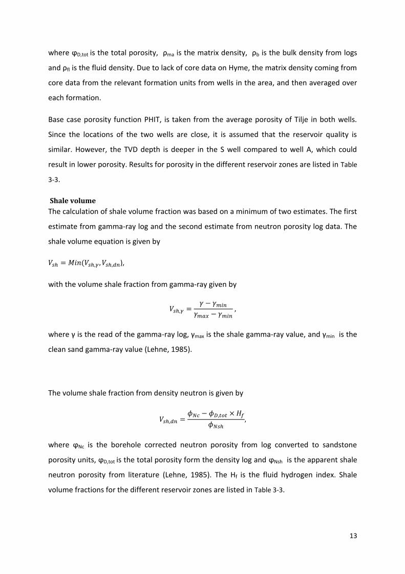
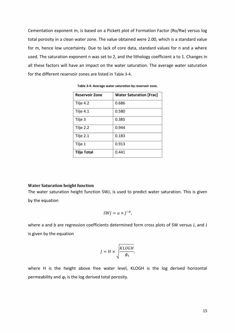
From Figure 3-2 and Figure 3-3 it can be observed that the Hyme field does not have a gas cap,
hence there exists no gas oil contact. Based on Figure 3-3, which shows a 3D cross section of
the reservoir, one can observe the base case oil water contact which is the boundary
between the oil saturated zone and water saturated zone.
Figure 3-2: 2D overview of the initial saturations on the Hyme field.
17
PVT
Based on fluid samples from Tilje formation, PVT data was measured and is reported in Table
3-6.
Table 3-6: PVT data from Tilje formation.
Parameter Value Unit
Solution GOR 187.3 Sm3/Sm3
Oil density 815.4 Kg/Sm3
Gas Gravity 1.1042 Kg/Sm3
Water Sp. Gravity 1.02841 Sp. Gravity
Water Salinity 41234.5 ppm
Oil formation volume factor 1.62884 Rm3/Sm3
Oil viscosity 0.214 cP
Reservoir temperature 96.5 ℃
Bubble point pressure 198.2 Bara
Figure 3-3: 3D cross section of the initial saturations on the Hyme field.

18
3.3 Hyme dynamic data
3.3.1 Faults
There have been interpreted four faults on Hyme based on seismic data, but only one of
them is integrated in the Hyme reference case, which is the internal fault G2. The internal
fault G2 is considered as the most important fault because this fault divides the reservoir
into two segments; western and eastern segment (Figure 2-2 and Figure 3-10). Other faults
were not included due to limited time and the importance of these faults was considered as
low.
For volume and recovery calculations, the location and sealing of the internal fault G2 is
crucial. The fault is interpreted on two picks. One pick in well 6407/8-5 A based on log
interpretation, and the other in well 6407/8-5 S based on image log results. Due to the bad
seismic, there is a lot of uncertainty connected to the fault location. However, the main
focus of this thesis will be the sealing capacity of the fault. The location will not be
investigated further. To account for the limited vertical resolution, the fault was extended to
a likely throw/length relationship.
Fault Seal
A fault seal analysis was performed by Statoil for investigating how fluids flow through the
internal fault. One of the objectives in the fault analysis was to calculate fault permeabilites
and exporting fault transmissibility multipliers to the reservoir simulator. Input data where
based on sample analysis of micro faults in core from analogue fields Njord and Heidrun. For
the Hyme reference case, the internal fault G2 is modeled with transmissibility multipliers
for each gridblock where the fault may exist. The internal fault G2 is assumed to be open in
the Hyme reference case.
3.3.3 Vertical communication Vertical communication is based on analogue data from Heidrun and Njord, where there is a
long production experience from the Tilje reservoir. According to Heidrun and Njord data,
there should be barriers or baffles to flow between most of the reservoir zones in Tilje. This
is most likely clay drapes and lenticular bedding (Reid et al., 1996). For the Hyme reference
case vertical communication between the reservoir zones in Tilje (Figure 3-4) is modeled
with transmissibility multipliers (Table 3-7).

19
Table 3-7: Transmissibility multipliers between the different reservoir zones.
From Figure 3-4 it can be observed that the transmissibility multipliers (Z1, Z2, Z3, Z4) are
applied on the boundaries between the different layers. There are vertical multipliers
between all zones, except between Tilje 2.1 and Tilje 1.2, where it is assumed to be
communication. Note that the multipliers in Table 3-7 are zero or really close to zero, which
implies no communication.
Transmissibility multiplier Reservoir zones [From-To] Multiplier value
Z1 Tilje 4.2- Tilje 4.1 0
Z2 Tilje 4.1- Tilje 3 0
Z3 Tilje 3 - Tilje 2.2 0.0001
Z4 Tilje 2.2- Tilje 2.1 0
Figure 3-4: Vertical cross section of the 3D Grid displaying the different reservoir zones, location of transmissibility multipliers (Z1, Z2, Z3, Z4), the two segments and the internal fault G2.
20
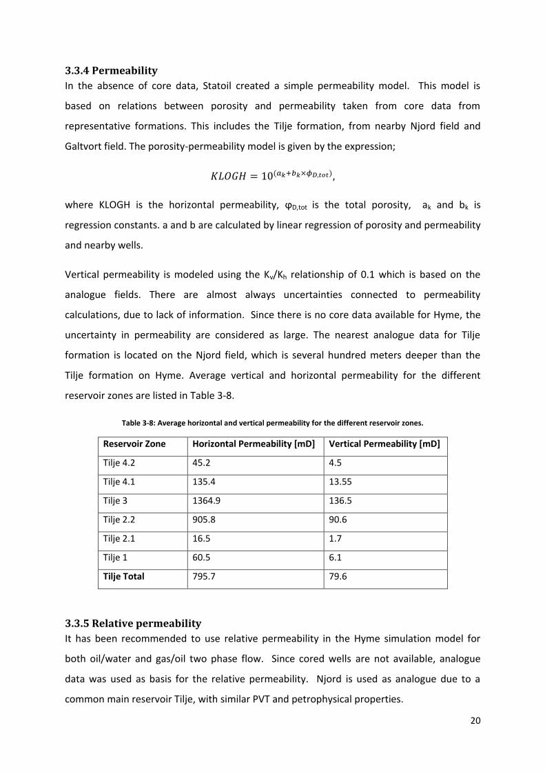
3.3.4 Permeability
In the absence of core data, Statoil created a simple permeability model. This model is
based on relations between porosity and permeability taken from core data from
representative formations. This includes the Tilje formation, from nearby Njord field and
Galtvort field. The porosity-permeability model is given by the expression;
( )
where KLOGH is the horizontal permeability, ϕD,tot is the total porosity, ak and bk is
regression constants. a and b are calculated by linear regression of porosity and permeability
and nearby wells.
Vertical permeability is modeled using the Kv/Kh relationship of 0.1 which is based on the
analogue fields. There are almost always uncertainties connected to permeability
calculations, due to lack of information. Since there is no core data available for Hyme, the
uncertainty in permeability are considered as large. The nearest analogue data for Tilje
formation is located on the Njord field, which is several hundred meters deeper than the
Tilje formation on Hyme. Average vertical and horizontal permeability for the different
reservoir zones are listed in Table 3-8.
Table 3-8: Average horizontal and vertical permeability for the different reservoir zones.
Reservoir Zone Horizontal Permeability [mD] Vertical Permeability [mD]
Tilje 4.2 45.2 4.5
Tilje 4.1 135.4 13.55
Tilje 3 1364.9 136.5
Tilje 2.2 905.8 90.6
Tilje 2.1 16.5 1.7
Tilje 1 60.5 6.1
Tilje Total 795.7 79.6
3.3.5 Relative permeability
It has been recommended to use relative permeability in the Hyme simulation model for
both oil/water and gas/oil two phase flow. Since cored wells are not available, analogue
data was used as basis for the relative permeability. Njord is used as analogue due to a
common main reservoir Tilje, with similar PVT and petrophysical properties.
21
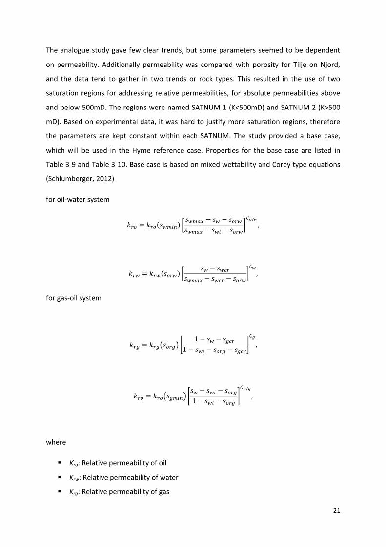
The analogue study gave few clear trends, but some parameters seemed to be dependent
on permeability. Additionally permeability was compared with porosity for Tilje on Njord,
and the data tend to gather in two trends or rock types. This resulted in the use of two
saturation regions for addressing relative permeabilities, for absolute permeabilities above
and below 500mD. The regions were named SATNUM 1 (K<500mD) and SATNUM 2 (K>500
mD). Based on experimental data, it was hard to justify more saturation regions, therefore
the parameters are kept constant within each SATNUM. The study provided a base case,
which will be used in the Hyme reference case. Properties for the base case are listed in
Table 3-9 and Table 3-10. Base case is based on mixed wettability and Corey type equations
(Schlumberger, 2012)
for oil-water system
( ) [
]
( ) [
]
for gas-oil system
( ) *
+
( ) *
+
where
Kro: Relative permeability of oil
Krw: Relative permeability of water
Krg: Relative permeability of gas
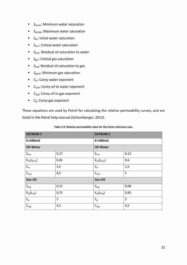
22
Swmin: Minimum water saturation
Swmax: Maximum water saturation
Swi: Initial water saturation
Swcr: Critical water saturation
Sorw: Residual oil saturation to water
Sgcr: Critical gas saturation
Sorg: Residual oil saturation to gas.
Sgmin: Minimum gas saturation.
Cw: Corey water exponent
Co/w: Corey oil to water exponent
Co/g: Corey oil to gas exponent
Cg: Corey gas exponent
These equations are used by Petrel for calculating the relative permeability curves, and are
listed in the Petrel help manual (Schlumberger, 2012).
Table 3-9: Relative permeability input for the Hyme reference case.
SATNUM 1 SATNUM 2
K<500mD K>500mD
Oil-Water Oil-Water
Sorw 0,17 Sorw 0,12
Krw(sorw) 0,45 Krw(sorw) 0,6
Cw 3,5 Cw 2,5
Co/w 4,5 Co/w 5
Gas-Oil Gas-Oil
Sorg 0,12 Sorg 0,08
Krg(sorg) 0,75 Krg(sorg) 0,85
Cg 2 Cg 2
Co/g 4,5 Co/g 4,5
23
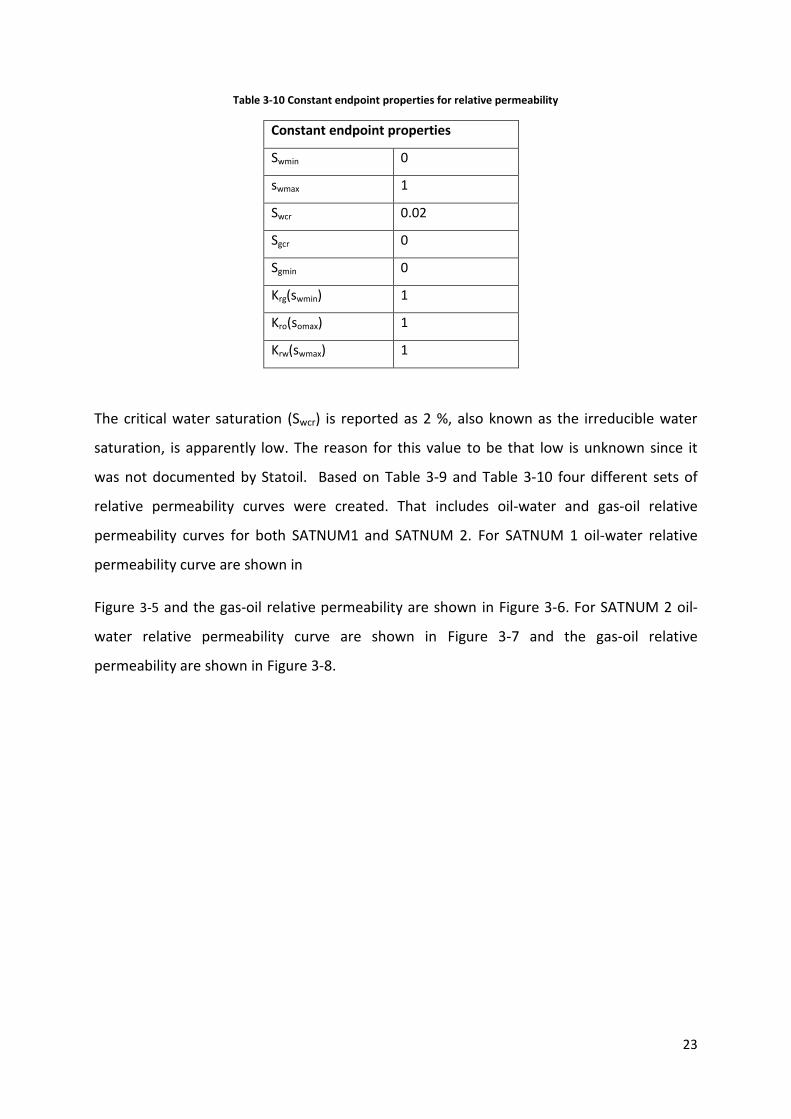
Table 3-10 Constant endpoint properties for relative permeability
Constant endpoint properties
Swmin 0
swmax 1
Swcr 0.02
Sgcr 0
Sgmin 0
Krg(swmin) 1
Kro(somax) 1
Krw(swmax) 1
The critical water saturation (Swcr) is reported as 2 %, also known as the irreducible water
saturation, is apparently low. The reason for this value to be that low is unknown since it
was not documented by Statoil. Based on Table 3-9 and Table 3-10 four different sets of
relative permeability curves were created. That includes oil-water and gas-oil relative
permeability curves for both SATNUM1 and SATNUM 2. For SATNUM 1 oil-water relative
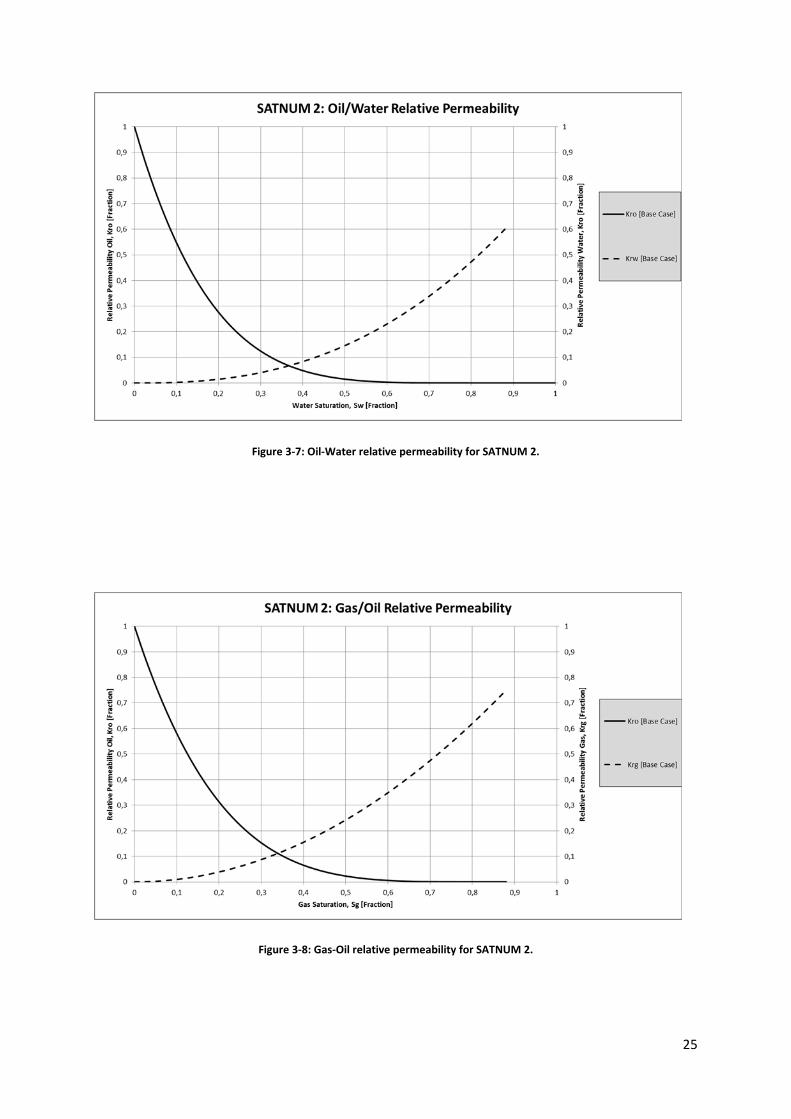
permeability curve are shown in
Figure 3-5 and the gas-oil relative permeability are shown in Figure 3-6. For SATNUM 2 oil-
water relative permeability curve are shown in Figure 3-7 and the gas-oil relative
permeability are shown in Figure 3-8.

24
Figure 3-5: Oil-Water relative permeability for SATNUM 1
Figure 3-6: Gas-Oil relative permeability for SATNUM 1
25
Figure 3-7: Oil-Water relative permeability for SATNUM 2.
Figure 3-8: Gas-Oil relative permeability for SATNUM 2.
26
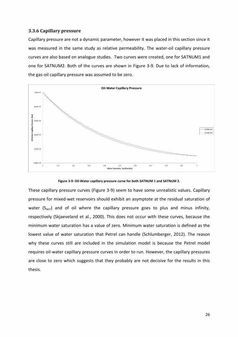
3.3.6 Capillary pressure
Capillary pressure are not a dynamic parameter, however it was placed in this section since it
was measured in the same study as relative permeability. The water-oil capillary pressure
curves are also based on analogue studies. Two curves were created, one for SATNUM1 and
one for SATNUM2. Both of the curves are shown in Figure 3-9. Due to lack of information,
the gas-oil capillary pressure was assumed to be zero.
Figure 3-9: Oil-Water capillary pressure curve for both SATNUM 1 and SATNUM 2.
These capillary pressure curves (Figure 3-9) seem to have some unrealistic values. Capillary
pressure for mixed-wet reservoirs should exhibit an asymptote at the residual saturation of
water (Swcr) and of oil where the capillary pressure goes to plus and minus infinity,
respectively (Skjaeveland et al., 2000). This does not occur with these curves, because the
minimum water saturation has a value of zero. Minimum water saturation is defined as the
lowest value of water saturation that Petrel can handle (Schlumberger, 2012). The reason
why these curves still are included in the simulation model is because the Petrel model
requires oil-water capillary pressure curves in order to run. However, the capillary pressures
are close to zero which suggests that they probably are not decisive for the results in this
thesis.
27
3.4 Hyme simulation model
3.4.1 Simulation Grid
A simulation grid for Hyme was created during the geological evaluation, and the grid
dimensions are given in Table 3-11.
Table 3-11: Grid dimensions for the Hyme reference case.
Direction X Y Z Total
Number of Gridblocks 77 114 156 1 369 368
Not all the gridblocks in Table 3-11 are active. An active gridblock can be defined as a
gridblock that has volume and where fluid can flow. There are 167 787 active gridblocks in
the model representing 12 % of the total gridblocks. To optimize the simulation run, a
keyword MINPV was used to remove small grid blocks that cause problems during the
simulation run. The keyword was set to remove gridblocks with a volume less than of 200
rm3. This caused a reduction of 13 170 grid blocks, which resulted in a STOIIP reduction of
1.8%. For the purpose of this study, this change is considered appropriate. This change
resulted in a total number of active gridblocks equal to 154 617.
3.4.2 In-Place volumes
To quantify the in-place volumes of Tilje, a static uncertainty study was performed by Statoil.
Structural, petrophysical, and PVT uncertainties were included. The study resulted in
determination of pore volume (PV), stock tank oil initially in place (STOIIP) and associated
gas. Due to the major fault (Figure 3-10), that divides the reservoirs into two segments,
results are divided into western and eastern segment (Table 3-12). Changes made by the
MINPV keyword are also included.
Table 3-12: In-place volumes for Hyme reference case
Segment Pore volume [106 Rm3] STOIIP [106 Sm3] Associated Gas [109 Sm3]
Western 39.96 8.13 1.52
Eastern 44.34 2.62 0.49
Total 84.30 10.75 2.01
28
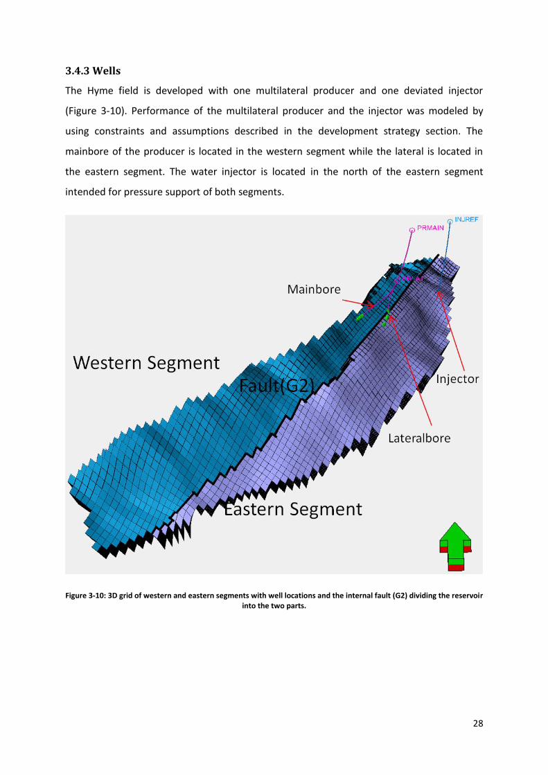
3.4.3 Wells
The Hyme field is developed with one multilateral producer and one deviated injector
(Figure 3-10). Performance of the multilateral producer and the injector was modeled by
using constraints and assumptions described in the development strategy section. The
mainbore of the producer is located in the western segment while the lateral is located in
the eastern segment. The water injector is located in the north of the eastern segment
intended for pressure support of both segments.
Figure 3-10: 3D grid of western and eastern segments with well locations and the internal fault (G2) dividing the reservoir into the two parts.

29
3.5 Development Strategy
Production start for Hyme was March 2nd 2013, with the multilateral producer as the only
active well. The water injector was at the time this study was performed, estimated to start
up 1st of June 2013. The simulation run will last until January 1st 2030. Both of the wells
where set up with rules based on constraints and assumptions provided by Statoil (Table
3-13).
Table 3-13: Well and production constraints
Constraint Unit Value
Platform back pressure production Bar 70
Platform water injection pressure Bar 290
Maximum oil production rate Sm3/d 2500
Maximum injection rate Sm3/d 5000
Maximum liquid production Sm3/d 4000
Maximum water production Sm3/d 3500
Maximum water cut lateral bore Sm3/sm3 0.70
A normal approach would be to generate lift curves for the different wells for controlling the
bottom hole pressures. For this study, the approach will be to use the constraints provided
by Statoil (Table 3-13). This includes the platform back pressure the producer needs to have
and the platform water injection pressure that constraints maximum injection rate. These
rules were implemented as well constraints.
The multilateral producer was assigned production rate constraints, which includes
maximum oil production rate, maximum water production rate and maximum total liquid
rate. On the lateral bore, a maximum water cut of 70 % was added for economic reasons.
Additionally, it was created a similar rule for the main bore. Here it was specified that
perforations with water cut greater than 95 % will shut in. For the water injector, a
maximum rate for injection was specified.
Additionally a group control was added to keep a stable reservoir pressure of 215 bar. This
rule will maintain the reservoir pressure on a field basis, and control the production and
injection to maintain this pressure. The aim of this rule is to avoid production below the
bubble point pressure, and still inject and produce at realistic rates.
30
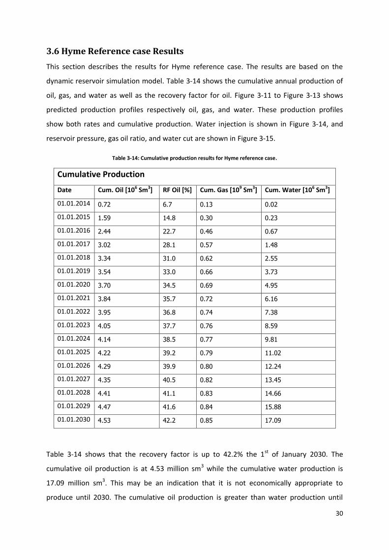
3.6 Hyme Reference case Results
This section describes the results for Hyme reference case. The results are based on the
dynamic reservoir simulation model. Table 3-14 shows the cumulative annual production of
oil, gas, and water as well as the recovery factor for oil. Figure 3-11 to Figure 3-13 shows
predicted production profiles respectively oil, gas, and water. These production profiles
show both rates and cumulative production. Water injection is shown in Figure 3-14, and
reservoir pressure, gas oil ratio, and water cut are shown in Figure 3-15.
Table 3-14: Cumulative production results for Hyme reference case.
Cumulative Production
Date Cum. Oil [106 Sm3] RF Oil [%] Cum. Gas [109 Sm3] Cum. Water [106 Sm3]
01.01.2014 0.72 6.7 0.13 0.02
01.01.2015 1.59 14.8 0.30 0.23
01.01.2016 2.44 22.7 0.46 0.67
01.01.2017 3.02 28.1 0.57 1.48
01.01.2018 3.34 31.0 0.62 2.55
01.01.2019 3.54 33.0 0.66 3.73
01.01.2020 3.70 34.5 0.69 4.95
01.01.2021 3.84 35.7 0.72 6.16
01.01.2022 3.95 36.8 0.74 7.38
01.01.2023 4.05 37.7 0.76 8.59
01.01.2024 4.14 38.5 0.77 9.81
01.01.2025 4.22 39.2 0.79 11.02
01.01.2026 4.29 39.9 0.80 12.24
01.01.2027 4.35 40.5 0.82 13.45
01.01.2028 4.41 41.1 0.83 14.66
01.01.2029 4.47 41.6 0.84 15.88
01.01.2030 4.53 42.2 0.85 17.09
Table 3-14 shows that the recovery factor is up to 42.2% the 1st of January 2030. The
cumulative oil production is at 4.53 million sm3 while the cumulative water production is
17.09 million sm3. This may be an indication that it is not economically appropriate to
produce until 2030. The cumulative oil production is greater than water production until
31
2019, where water production is rising dramatically. Given that Hyme is classified as a fast
track development, it is not believed that the depletion will last as far as 2030, which these
results support.
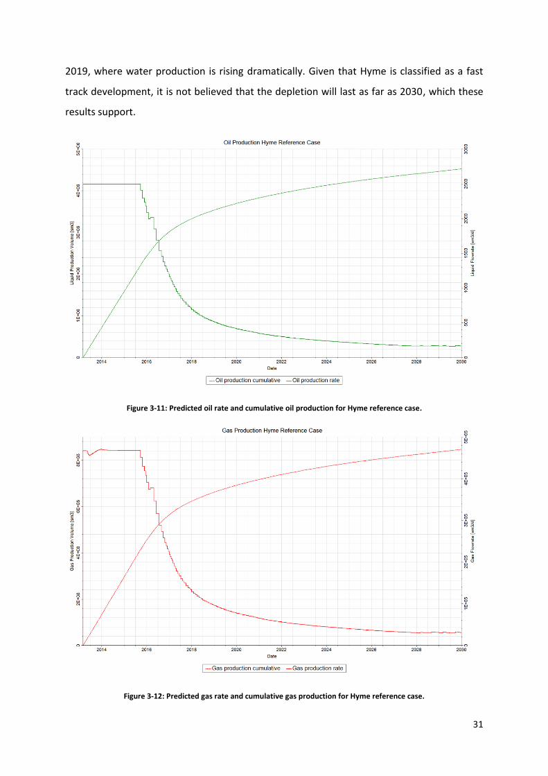
Figure 3-11: Predicted oil rate and cumulative oil production for Hyme reference case.
Figure 3-12: Predicted gas rate and cumulative gas production for Hyme reference case.
32
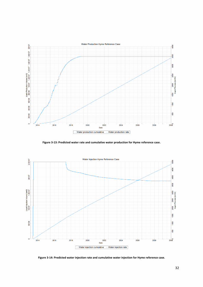
Figure 3-13: Predicted water rate and cumulative water production for Hyme reference case.
Figure 3-14: Predicted water injection rate and cumulative water injection for Hyme reference case.
33
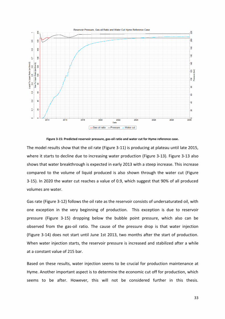
Figure 3-15: Predicted reservoir pressure, gas-oil ratio and water cut for Hyme reference case.
The model results show that the oil rate (Figure 3-11) is producing at plateau until late 2015,
where it starts to decline due to increasing water production (Figure 3-13). Figure 3-13 also
shows that water breakthrough is expected in early 2013 with a steep increase. This increase
compared to the volume of liquid produced is also shown through the water cut (Figure
3-15). In 2020 the water cut reaches a value of 0.9, which suggest that 90% of all produced
volumes are water.
Gas rate (Figure 3-12) follows the oil rate as the reservoir consists of undersaturated oil, with
one exception in the very beginning of production. This exception is due to reservoir
pressure (Figure 3-15) dropping below the bubble point pressure, which also can be
observed from the gas-oil ratio. The cause of the pressure drop is that water injection
(Figure 3-14) does not start until June 1st 2013, two months after the start of production.
When water injection starts, the reservoir pressure is increased and stabilized after a while
at a constant value of 215 bar.
Based on these results, water injection seems to be crucial for production maintenance at
Hyme. Another important aspect is to determine the economic cut off for production, which
seems to be after. However, this will not be considered further in this thesis.

34
4. Pre-production Uncertainty Study
A pre-production uncertainty study is performed based on the Hyme reference case. The
first objective was to determine the uncertainty parameters of interest. The parameters
chosen are parameters that are interpreted as uncertain, and with possibility to make a
significant difference in terms of oil recovery and oil volume in-place. These parameters
were provided by Statoil including the ranges for the uncertainty.
The next objective was to create an uncertainty workflow (Figure 4-1) in the Petrel software
where the interpreted uncertainty ranges are integrated. From this workflow, sensitivities
were generated based on the low and high cases for the interpreted uncertainty ranges. This
generated 20 simulation cases that provided an overview of which parameters that are
affecting the oil volumes in-place and the cumulative oil production and how much the
impact is.
When the 20 sensitivity simulations were performed, a stochastic Monte Carlo based
uncertainty study was made, where random selections of the parameters were combined in
several simulation runs. In this study, 200 simulation cases were generated. The results from
this study will aid in the understanding of the future performance and potential of Hyme.
4.0.1 Stochastic modeling
Almost all data used in reservoir simulation are uncertain. These uncertainties tend to be
large, specifically away from the wells to spatially distribution parameters such as porosity
and permeability. A consequence of this is that a production profile associated with any
development scheme cannot be predicted exactly. In order to capture the behavior of the
reservoir, the best thing to do is calculate a range of possible profiles (O.J Lèpine et al.,
1999). For the Hyme reference case, only one production profile is obtained. In order to
capture what impact different uncertainties will have on oil production and oil volume in
place, a stochastic uncertainty study was performed.
Initially, a reservoir can be considered as deterministic. This means that the reservoir exists,
and it has input parameters that can be observed and measured. Haldorsen and Damsleth
presented a definition of stochastic phenomenon or variable in the JPT paper “Stochastic
Modeling” April 1990: “A stochastic phenomenon or variable is characterized by the
35
property that a given set of circumstances does not always lead to the same outcome (so
that there is no deterministic regularity) but to different outcomes in such a way that there
is statistical regularity.” An example would be; if we had used deterministic values for the
input parameters in a reservoir description, we would obtain one answer. In this case, this
would be Hyme reference case. Applying stochastic techniques enables the user to achieve
uncertainty ranges. This can be considered as crucial to understand the subsurface with
limited amount of data, which is the case for Hyme (Haldorsen and Damsleth, 1990).
The main reason for applying stochastic techniques is that we know that there are a lot of
unknowns in the subsurface. Incomplete information about dimensions and geologic
structures are a major reason. Another reason is spatial variations and distributions in the
reservoir, which is really hard to predict. The parameters of interest can be divided into
static and dynamic parameters. Static parameters can be considered as point values along
the well, combined with seismic data, while dynamic parameters are time-dependent
parameters such as pressure and rates. There could also be unknown relationships between
the different petro physical input parameters and the volume of rock used for averaging
(Haldorsen and Damsleth, 1990). Summarized, the main problem is that it exist a gap
between observed and unsampled locations. In order to perform this stochastic uncertainty
study, a Monte Carlo sampling approach will be used.
4.0.2 Monte Carlo sampling
Monte Carlo method can be defined as a study of a stochastic model which simulates, in all
essential aspect, a physical or mathematical process. The method is a combination of
sampling theory and numerical analysis, which gives the method a special contribution to
the science of computing. This implies that Monte Carlo is a practical method that can solve
problems by numerical operations on random numbers (Stoian, 1965). As mentioned, Statoil
provided interpreted uncertainty ranges for some of the input parameters in Hyme
reference model. These parameters will be further discussed in the uncertainty parameter
section 4.1. By using Monte Carlo simulation, random values within these ranges will be
sampled. This means that several simulation cases will be generated and run based on
random sampling within each of the uncertainty ranges.
36
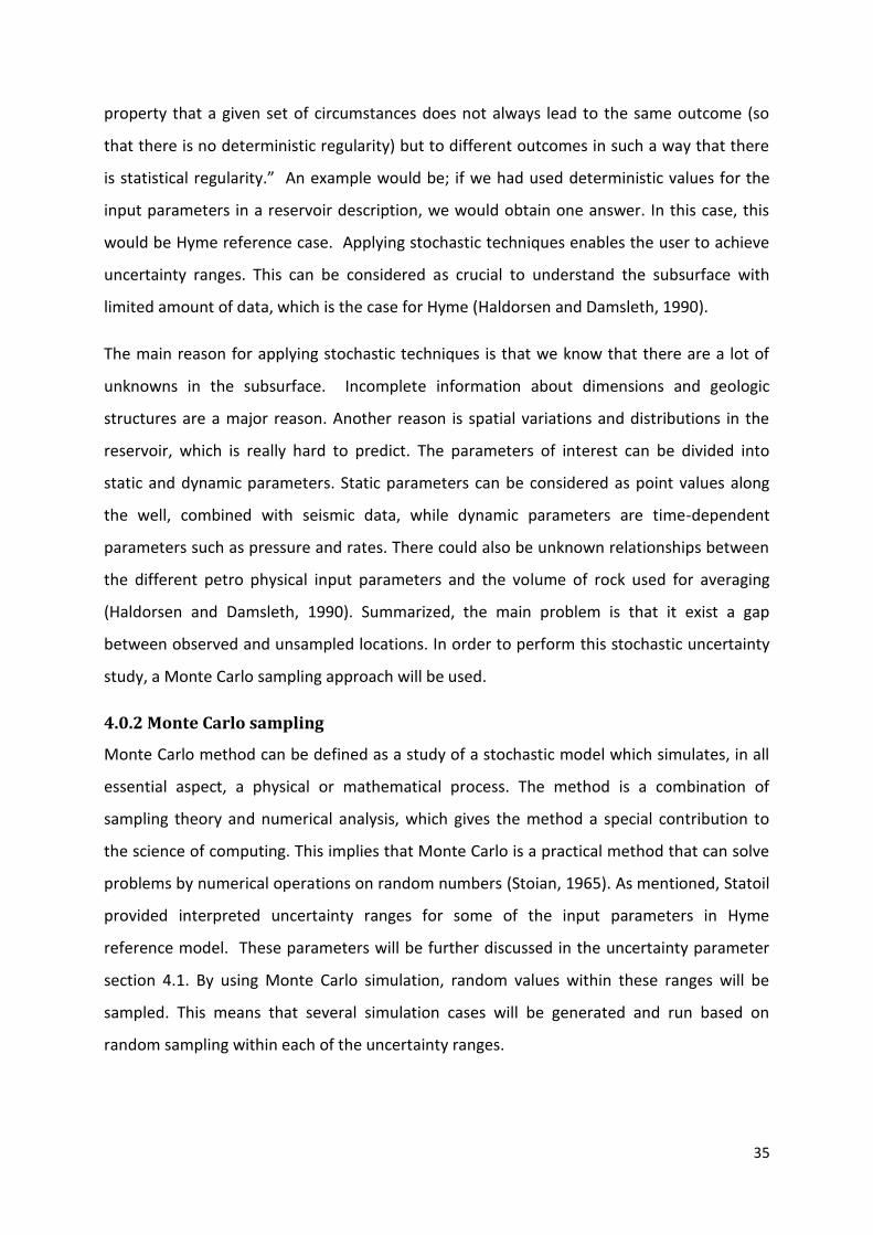
4.0.2 Workflow for Pre-production uncertainty study
Figure 4-1: Schematic overview of pre-production uncertainty study.
37
4.1 Uncertainty Parameters
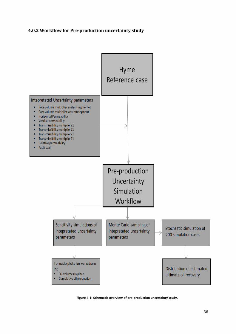
4.1.1 In-Place volumes
As input to the uncertainty study being performed, a pore volume uncertainty range will be
used. The reason for this is to keep the volume calculation simple, without dependency of
water saturation and formation volume factor. Pore volume is a function of gross rock
volume (GRV), porosity and net to gross (NTG);
.
Based on the uncertainty study performed by Statoil described in section 3.4.2, uncertainty
ranges for this parameter were generated with respect to both eastern and western
segment (Table 4-1).
Table 4-1: Uncertainty ranges for pore volume multipliers for eastern and western segment.
Pore volume multiplier Low Reference High Description
Eastern segment 0.5 1 1.62 Multiplier value
Western segment 0.2 1 1.4 Multiplier value
Notice that the uncertainties are multipliers, not actual volumes. The reason for using
multipliers instead of actual volumes is for simplicity for input into the simulation model. In
terms of volumes, the ranges will be as shown in Table 4-2.
Table 4-2: Uncertainty ranges for pore volume in eastern and western segment.
Pore volume Low Reference High Unit
Eastern segment 22.17 44.34 71.83 PV [106 Rm3]
Western segment 7.99 39.96 55.94 PV [106 Rm3]
The pore volume multipliers Table 4-1 will affect the stock tank oil initially in-place.
However, as described in section 3.4.2, the oil in-place is much larger in the western
segment compared to the eastern segment, even though the pore volume is significantly
larger in eastern segment. This can be explained by that the initial oil saturation is larger in
western segment (Figure 3-3).
38
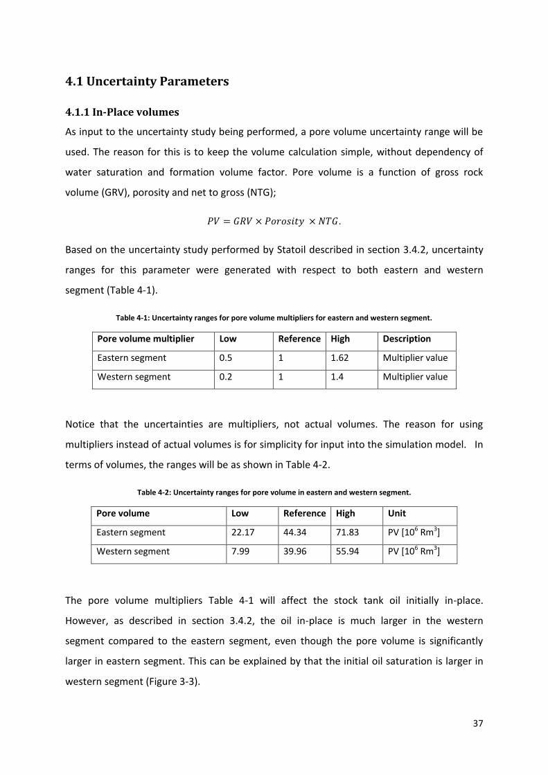
4.1.2 Permeability
Based on the petrophysical evaluation of vertical and horizontal permeability, uncertainty
ranges for the entire Tilje formation was interpreted (Table 4-3).
Table 4-3: Uncertainty ranges for horizontal and vertical permeability in the Tilje formation.
Parameter Low Reference High Case Unit
Horizontal Permeability 159.1 795.7 3978.5 [mD]
Vertical Permeability 15.9 79.6 397.9 [mD]
Table 4-3 shows that the uncertainty range for permeability in Tilje is large, and hence
important for this study. To apply these ranges to the uncertainty simulation study,
multipliers were created based on low, reference and high cases (Table 4-4).
Table 4-4: Uncertainty ranges for horizontal and vertical permeability multipliers in the Tilje formation.
Parameter Low Reference High Descriptiom
Horizontal Permeability 0.2 1 5 Multiplier value
Vertical permeability 0.01 0.1 0.6 Multiplier value
4.1.3 Relative permeability
As mentioned in section 3.3.5, Statoil performed an analogue study to determine the
relative permeability. The study provided a base, high, and low case. Base case is based on
mixed wettability and the optimistic case based on water-wet sand, with the pessimistic case
based on oil-wet sand. The properties are given in Table 4-5.
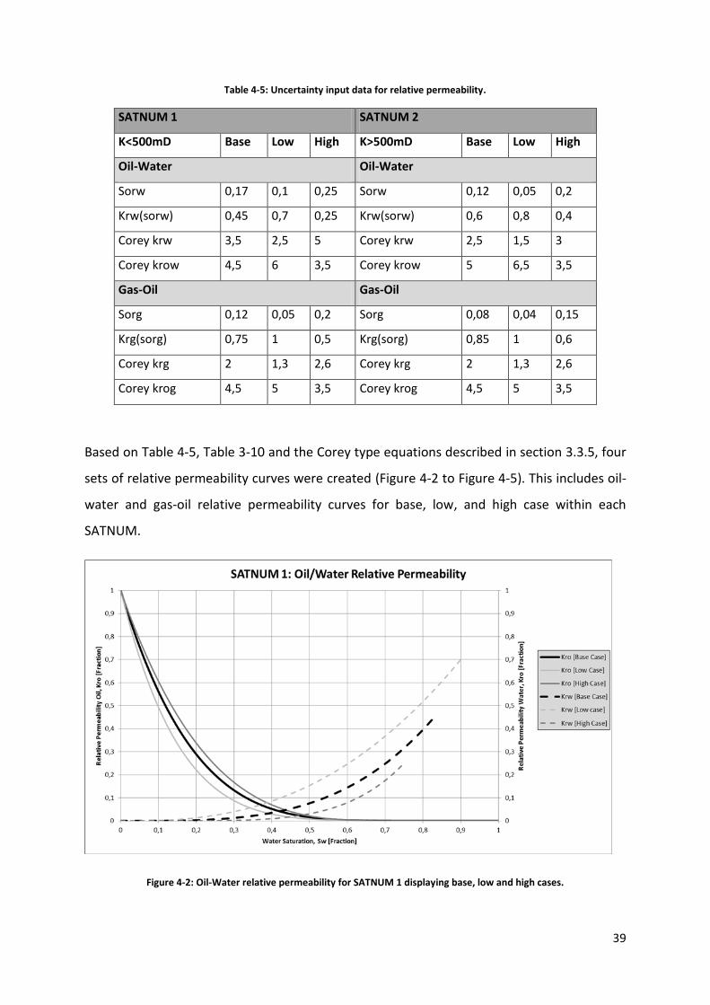
39
Table 4-5: Uncertainty input data for relative permeability.
SATNUM 1 SATNUM 2
K<500mD Base Low High K>500mD Base Low High
Oil-Water Oil-Water
Sorw 0,17 0,1 0,25 Sorw 0,12 0,05 0,2
Krw(sorw) 0,45 0,7 0,25 Krw(sorw) 0,6 0,8 0,4
Corey krw 3,5 2,5 5 Corey krw 2,5 1,5 3
Corey krow 4,5 6 3,5 Corey krow 5 6,5 3,5
Gas-Oil Gas-Oil
Sorg 0,12 0,05 0,2 Sorg 0,08 0,04 0,15
Krg(sorg) 0,75 1 0,5 Krg(sorg) 0,85 1 0,6
Corey krg 2 1,3 2,6 Corey krg 2 1,3 2,6
Corey krog 4,5 5 3,5 Corey krog 4,5 5 3,5
Based on Table 4-5, Table 3-10 and the Corey type equations described in section 3.3.5, four
sets of relative permeability curves were created (Figure 4-2 to Figure 4-5). This includes oil-
water and gas-oil relative permeability curves for base, low, and high case within each
SATNUM.
Figure 4-2: Oil-Water relative permeability for SATNUM 1 displaying base, low and high cases.
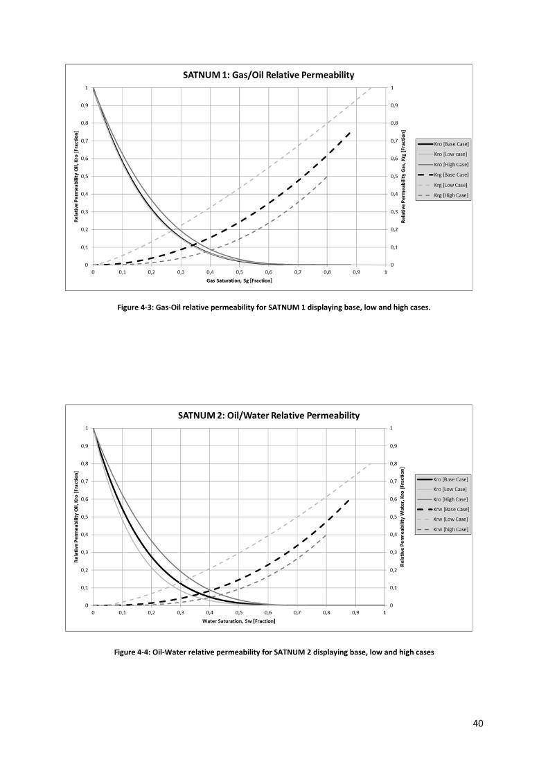
40
Figure 4-3: Gas-Oil relative permeability for SATNUM 1 displaying base, low and high cases.
Figure 4-4: Oil-Water relative permeability for SATNUM 2 displaying base, low and high cases
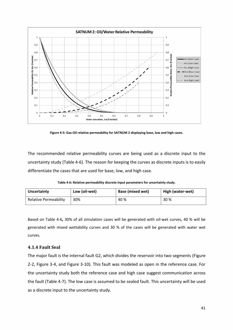
41
Figure 4-5: Gas-Oil relative permeability for SATNUM 2 displaying base, low and high cases.
The recommended relative permeability curves are being used as a discrete input to the
uncertainty study (Table 4-6). The reason for keeping the curves as discrete inputs is to easily
differentiate the cases that are used for base, low, and high case.
Table 4-6: Relative permeability discrete input parameters for uncertainty study.
Uncertainty Low (oil-wet) Base (mixed wet) High (water-wet)
Relative Permeability 30% 40 % 30 %
Based on Table 4-6, 30% of all simulation cases will be generated with oil-wet curves, 40 % will be
generated with mixed wettability curves and 30 % of the cases will be generated with water wet
curves.
4.1.4 Fault Seal
The major fault is the internal fault G2, which divides the reservoir into two segments (Figure
2-2, Figure 3-4, and Figure 3-10). This fault was modeled as open in the reference case. For
the uncertainty study both the reference case and high case suggest communication across
the fault (Table 4-7). The low case is assumed to be sealed fault. This uncertainty will be used
as a discrete input to the uncertainty study.
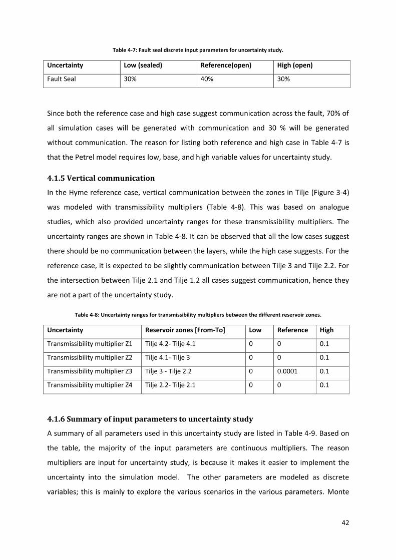
42
Table 4-7: Fault seal discrete input parameters for uncertainty study.
Uncertainty Low (sealed) Reference(open) High (open)
Fault Seal 30% 40% 30%
Since both the reference case and high case suggest communication across the fault, 70% of
all simulation cases will be generated with communication and 30 % will be generated
without communication. The reason for listing both reference and high case in Table 4-7 is
that the Petrel model requires low, base, and high variable values for uncertainty study.
4.1.5 Vertical communication In the Hyme reference case, vertical communication between the zones in Tilje (Figure 3-4)
was modeled with transmissibility multipliers (Table 4-8). This was based on analogue
studies, which also provided uncertainty ranges for these transmissibility multipliers. The
uncertainty ranges are shown in Table 4-8. It can be observed that all the low cases suggest
there should be no communication between the layers, while the high case suggests. For the
reference case, it is expected to be slightly communication between Tilje 3 and Tilje 2.2. For
the intersection between Tilje 2.1 and Tilje 1.2 all cases suggest communication, hence they
are not a part of the uncertainty study.
Table 4-8: Uncertainty ranges for transmissibility multipliers between the different reservoir zones.
Uncertainty Reservoir zones [From-To] Low Reference High
Transmissibility multiplier Z1 Tilje 4.2- Tilje 4.1 0 0 0.1
Transmissibility multiplier Z2 Tilje 4.1- Tilje 3 0 0 0.1
Transmissibility multiplier Z3 Tilje 3 - Tilje 2.2 0 0.0001 0.1
Transmissibility multiplier Z4 Tilje 2.2- Tilje 2.1 0 0 0.1
4.1.6 Summary of input parameters to uncertainty study
A summary of all parameters used in this uncertainty study are listed in Table 4-9. Based on
the table, the majority of the input parameters are continuous multipliers. The reason
multipliers are input for uncertainty study, is because it makes it easier to implement the
uncertainty into the simulation model. The other parameters are modeled as discrete
variables; this is mainly to explore the various scenarios in the various parameters. Monte
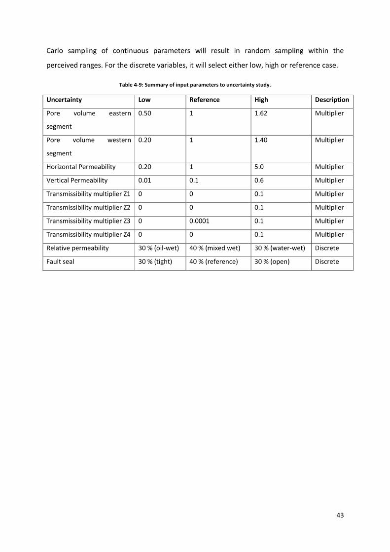
43
Carlo sampling of continuous parameters will result in random sampling within the
perceived ranges. For the discrete variables, it will select either low, high or reference case.
Table 4-9: Summary of input parameters to uncertainty study.
Uncertainty Low Reference High Description
Pore volume eastern
segment
0.50 1 1.62 Multiplier
Pore volume western
segment
0.20 1 1.40 Multiplier
Horizontal Permeability 0.20 1 5.0 Multiplier
Vertical Permeability 0.01 0.1 0.6 Multiplier
Transmissibility multiplier Z1 0 0 0.1 Multiplier
Transmissibility multiplier Z2 0 0 0.1 Multiplier
Transmissibility multiplier Z3 0 0.0001 0.1 Multiplier
Transmissibility multiplier Z4 0 0 0.1 Multiplier
Relative permeability 30 % (oil-wet) 40 % (mixed wet) 30 % (water-wet) Discrete
Fault seal 30 % (tight) 40 % (reference) 30 % (open) Discrete
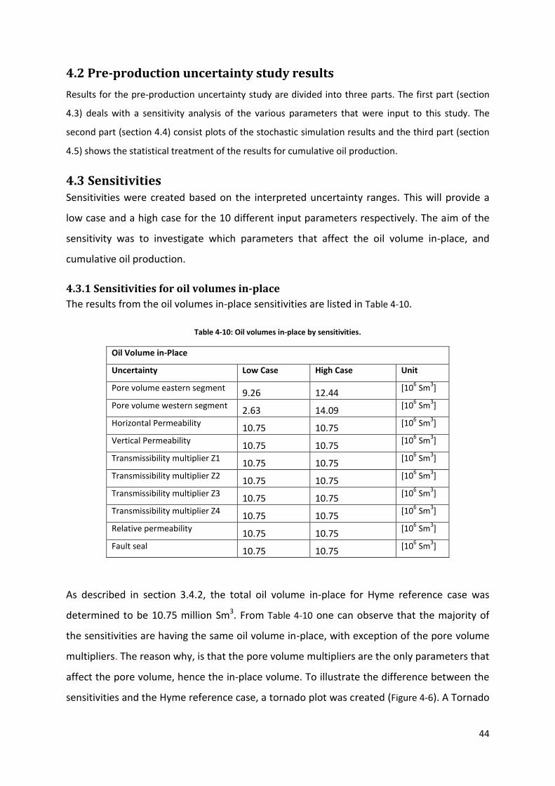
44
4.2 Pre-production uncertainty study results
Results for the pre-production uncertainty study are divided into three parts. The first part (section
4.3) deals with a sensitivity analysis of the various parameters that were input to this study. The
second part (section 4.4) consist plots of the stochastic simulation results and the third part (section
4.5) shows the statistical treatment of the results for cumulative oil production.
4.3 Sensitivities Sensitivities were created based on the interpreted uncertainty ranges. This will provide a
low case and a high case for the 10 different input parameters respectively. The aim of the
sensitivity was to investigate which parameters that affect the oil volume in-place, and
cumulative oil production.
4.3.1 Sensitivities for oil volumes in-place
The results from the oil volumes in-place sensitivities are listed in Table 4-10.
Table 4-10: Oil volumes in-place by sensitivities.
Oil Volume in-Place
Uncertainty Low Case High Case Unit
Pore volume eastern segment 9.26 12.44
[106 Sm
3]
Pore volume western segment 2.63 14.09
[106 Sm
3]
Horizontal Permeability 10.75 10.75
[106 Sm
3]
Vertical Permeability 10.75 10.75
[106 Sm
3]
Transmissibility multiplier Z1 10.75 10.75
[106 Sm
3]
Transmissibility multiplier Z2 10.75 10.75
[106 Sm
3]
Transmissibility multiplier Z3 10.75 10.75
[106 Sm
3]
Transmissibility multiplier Z4 10.75 10.75
[106 Sm
3]
Relative permeability 10.75 10.75
[106 Sm
3]
Fault seal 10.75 10.75
[106 Sm
3]
As described in section 3.4.2, the total oil volume in-place for Hyme reference case was
determined to be 10.75 million Sm3. From Table 4-10 one can observe that the majority of
the sensitivities are having the same oil volume in-place, with exception of the pore volume
multipliers. The reason why, is that the pore volume multipliers are the only parameters that
affect the pore volume, hence the in-place volume. To illustrate the difference between the
sensitivities and the Hyme reference case, a tornado plot was created (Figure 4-6). A Tornado
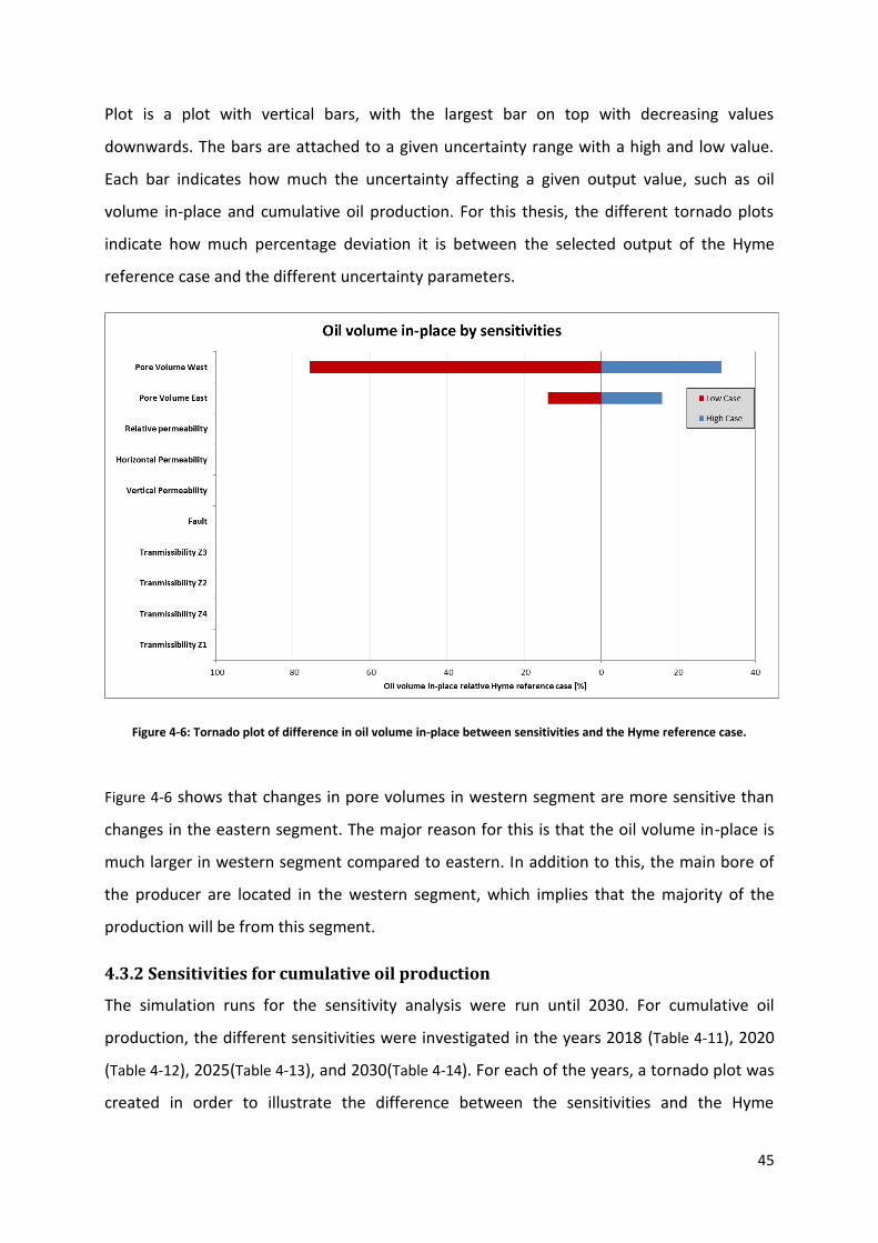
45
Plot is a plot with vertical bars, with the largest bar on top with decreasing values
downwards. The bars are attached to a given uncertainty range with a high and low value.
Each bar indicates how much the uncertainty affecting a given output value, such as oil
volume in-place and cumulative oil production. For this thesis, the different tornado plots
indicate how much percentage deviation it is between the selected output of the Hyme
reference case and the different uncertainty parameters.
Figure 4-6: Tornado plot of difference in oil volume in-place between sensitivities and the Hyme reference case.
Figure 4-6 shows that changes in pore volumes in western segment are more sensitive than
changes in the eastern segment. The major reason for this is that the oil volume in-place is
much larger in western segment compared to eastern. In addition to this, the main bore of
the producer are located in the western segment, which implies that the majority of the
production will be from this segment.
4.3.2 Sensitivities for cumulative oil production
The simulation runs for the sensitivity analysis were run until 2030. For cumulative oil
production, the different sensitivities were investigated in the years 2018 (Table 4-11), 2020
(Table 4-12), 2025(Table 4-13), and 2030(Table 4-14). For each of the years, a tornado plot was
created in order to illustrate the difference between the sensitivities and the Hyme
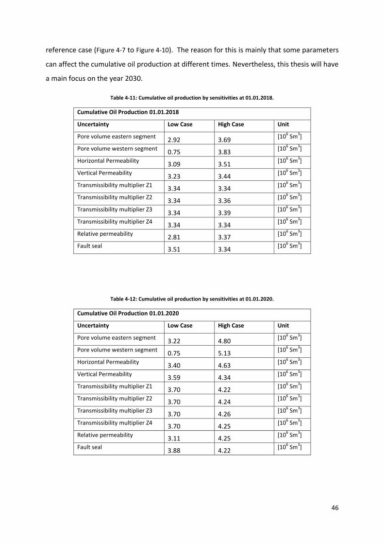
46
reference case (Figure 4-7 to Figure 4-10). The reason for this is mainly that some parameters
can affect the cumulative oil production at different times. Nevertheless, this thesis will have
a main focus on the year 2030.
Table 4-11: Cumulative oil production by sensitivities at 01.01.2018.
Cumulative Oil Production 01.01.2018
Uncertainty Low Case High Case Unit
Pore volume eastern segment 2.92 3.69
[106 Sm
3]
Pore volume western segment 0.75 3.83
[106 Sm
3]
Horizontal Permeability 3.09 3.51
[106 Sm
3]
Vertical Permeability 3.23 3.44
[106 Sm
3]
Transmissibility multiplier Z1 3.34 3.34
[106 Sm
3]
Transmissibility multiplier Z2 3.34 3.36
[106 Sm
3]
Transmissibility multiplier Z3 3.34 3.39
[106 Sm
3]
Transmissibility multiplier Z4 3.34 3.34
[106 Sm
3]
Relative permeability 2.81 3.37
[106 Sm
3]
Fault seal 3.51 3.34
[106 Sm
3]
Table 4-12: Cumulative oil production by sensitivities at 01.01.2020.
Cumulative Oil Production 01.01.2020
Uncertainty Low Case High Case Unit
Pore volume eastern segment 3.22 4.80
[106 Sm
3]
Pore volume western segment 0.75 5.13
[106 Sm
3]
Horizontal Permeability 3.40 4.63
[106 Sm
3]
Vertical Permeability 3.59 4.34
[106 Sm
3]
Transmissibility multiplier Z1 3.70 4.22
[106 Sm
3]
Transmissibility multiplier Z2 3.70 4.24
[106 Sm
3]
Transmissibility multiplier Z3 3.70 4.26
[106 Sm
3]
Transmissibility multiplier Z4 3.70 4.25
[106 Sm
3]
Relative permeability 3.11 4.25
[106 Sm
3]
Fault seal 3.88 4.22
[106 Sm
3]

47
Table 4-13: Cumulative oil production by sensitivities at 01.01.2025.
Cumulative Oil Production 01.01.2025
Uncertainty Low Case High Case Unit
Pore volume eastern segment 3.66 4,80
[106 Sm
3]
Pore volume western segment 0.75 5.13
[106 Sm
3]
Horizontal Permeability 3.85 4.63
[106 Sm
3]
Vertical Permeability 4.09 4.34
[106 Sm
3]
Transmissibility multiplier Z1 4.22 4.22
[106 Sm
3]
Transmissibility multiplier Z2 4.22 4.24
[106 Sm
3]
Transmissibility multiplier Z3 4.22 4.26
[106 Sm
3]
Transmissibility multiplier Z4 4.22 4.25
[106 Sm
3]
Relative permeability 3.56 4.25
[106 Sm
3]
Fault seal 4.39 4.22
[106 Sm
3]
Table 4-14: Cumulative oil production by sensitivities at 01.01.2030.
Cumulative Oil Production 01.01.2030
Uncertainty Low Case High Case Unit
Pore volume eastern segment 3.97 5.15
[106 Sm
3]
Pore volume western segment 0.75 5.55
[106 Sm
3]
Horizontal Permeability 4.17 4.96
[106 Sm
3]
Vertical Permeability 4.40 4.65
[106 Sm
3]
Transmissibility multiplier Z1 4.53 4.53
[106 Sm
3]
Transmissibility multiplier Z2 4.53 4.55
[106 Sm
3]
Transmissibility multiplier Z3 4.53 4.58
[106 Sm
3]
Transmissibility multiplier Z4 4.53 4.57
[106 Sm
3]
Relative permeability 3.86 4.56
[106 Sm
3]
Fault seal 4.70 4.53
[106 Sm
3]

48
Figure 4-7: Tornado plot of difference in cumulative oil production between sensitivities and the Hyme reference case at 01.01.2018.
Figure 4-8: Tornado plot of difference in cumulative oil production between sensitivities and the Hyme reference case at 01.01.2020.

49
Figure 4-9: Tornado plot of difference in cumulative oil production between sensitivities and the Hyme reference case at 01.01.2025.
Figure 4-10: Tornado plot of difference in umulative oil production between sensitivities and the Hyme reference case at 01.01.2030.
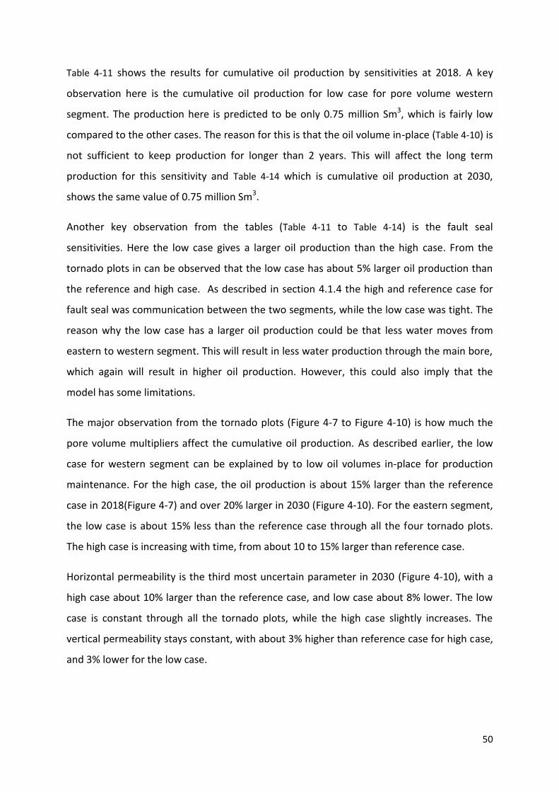
50
Table 4-11 shows the results for cumulative oil production by sensitivities at 2018. A key
observation here is the cumulative oil production for low case for pore volume western
segment. The production here is predicted to be only 0.75 million Sm3, which is fairly low
compared to the other cases. The reason for this is that the oil volume in-place (Table 4-10) is
not sufficient to keep production for longer than 2 years. This will affect the long term
production for this sensitivity and Table 4-14 which is cumulative oil production at 2030,
shows the same value of 0.75 million Sm3.
Another key observation from the tables (Table 4-11 to Table 4-14) is the fault seal
sensitivities. Here the low case gives a larger oil production than the high case. From the
tornado plots in can be observed that the low case has about 5% larger oil production than
the reference and high case. As described in section 4.1.4 the high and reference case for
fault seal was communication between the two segments, while the low case was tight. The
reason why the low case has a larger oil production could be that less water moves from
eastern to western segment. This will result in less water production through the main bore,
which again will result in higher oil production. However, this could also imply that the
model has some limitations.
The major observation from the tornado plots (Figure 4-7 to Figure 4-10) is how much the
pore volume multipliers affect the cumulative oil production. As described earlier, the low
case for western segment can be explained by to low oil volumes in-place for production
maintenance. For the high case, the oil production is about 15% larger than the reference
case in 2018(Figure 4-7) and over 20% larger in 2030 (Figure 4-10). For the eastern segment,
the low case is about 15% less than the reference case through all the four tornado plots.
The high case is increasing with time, from about 10 to 15% larger than reference case.
Horizontal permeability is the third most uncertain parameter in 2030 (Figure 4-10), with a
high case about 10% larger than the reference case, and low case about 8% lower. The low
case is constant through all the tornado plots, while the high case slightly increases. The
vertical permeability stays constant, with about 3% higher than reference case for high case,
and 3% lower for the low case.

51
The relative permeability has a large influence when it comes to low case. It is constant
through all tornado plots on a value about 17% lower than the reference case. The high case
is slightly higher than reference case, about 1%.
For the vertical transmissibility multipliers, the difference between the reference case and
the sensitivities is low. The largest difference is the transmissibility Z3 which is between the
layers Tilje 3 and Tilje 2.2, with a high case about 1% higher than the reference case. A major
reason for these results could be that the high case multipliers can be considered as low
(Table 4-8), hence the communication is low.
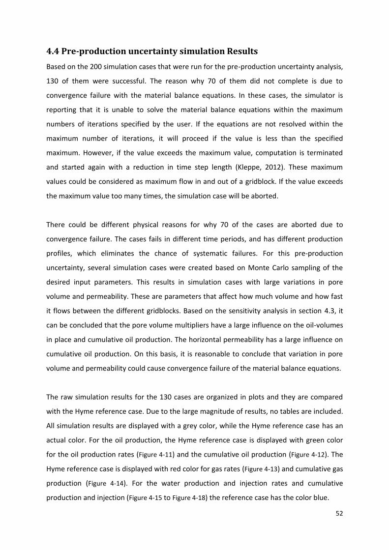
52
4.4 Pre-production uncertainty simulation Results
Based on the 200 simulation cases that were run for the pre-production uncertainty analysis,
130 of them were successful. The reason why 70 of them did not complete is due to
convergence failure with the material balance equations. In these cases, the simulator is
reporting that it is unable to solve the material balance equations within the maximum
numbers of iterations specified by the user. If the equations are not resolved within the
maximum number of iterations, it will proceed if the value is less than the specified
maximum. However, if the value exceeds the maximum value, computation is terminated
and started again with a reduction in time step length (Kleppe, 2012). These maximum
values could be considered as maximum flow in and out of a gridblock. If the value exceeds
the maximum value too many times, the simulation case will be aborted.
There could be different physical reasons for why 70 of the cases are aborted due to
convergence failure. The cases fails in different time periods, and has different production
profiles, which eliminates the chance of systematic failures. For this pre-production
uncertainty, several simulation cases were created based on Monte Carlo sampling of the
desired input parameters. This results in simulation cases with large variations in pore
volume and permeability. These are parameters that affect how much volume and how fast
it flows between the different gridblocks. Based on the sensitivity analysis in section 4.3, it
can be concluded that the pore volume multipliers have a large influence on the oil-volumes
in place and cumulative oil production. The horizontal permeability has a large influence on
cumulative oil production. On this basis, it is reasonable to conclude that variation in pore
volume and permeability could cause convergence failure of the material balance equations.
The raw simulation results for the 130 cases are organized in plots and they are compared
with the Hyme reference case. Due to the large magnitude of results, no tables are included.
All simulation results are displayed with a grey color, while the Hyme reference case has an
actual color. For the oil production, the Hyme reference case is displayed with green color
for the oil production rates (Figure 4-11) and the cumulative oil production (Figure 4-12). The
Hyme reference case is displayed with red color for gas rates (Figure 4-13) and cumulative gas
production (Figure 4-14). For the water production and injection rates and cumulative
production and injection (Figure 4-15 to Figure 4-18) the reference case has the color blue.
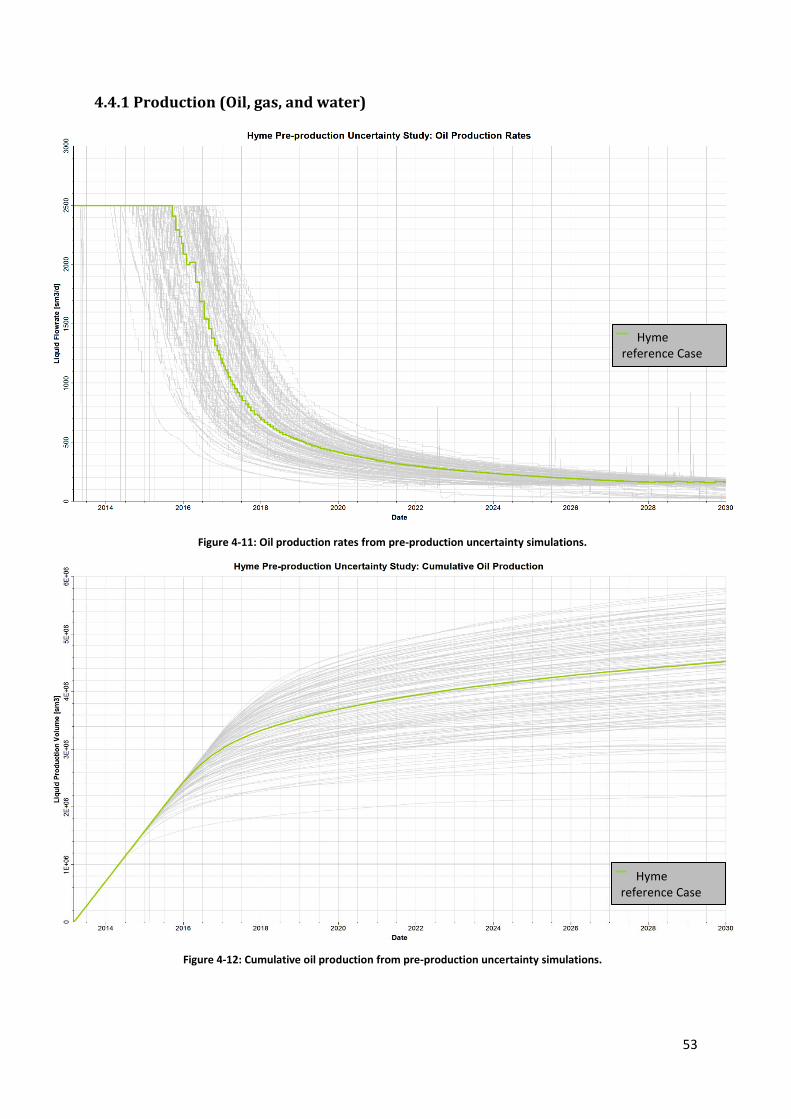
53
4.4.1 Production (Oil, gas, and water)
4.4.1 Gas production
Hyme reference Case
Hyme reference Case
Figure 4-11: Oil production rates from pre-production uncertainty simulations.
Figure 4-12: Cumulative oil production from pre-production uncertainty simulations.
54
Hyme reference Case
Hyme reference Case
Figure 4-13: Gas production rates from pre-production uncertainty simulations
Figure 4-14: Cumulative gas production from pre-production uncertainty simulations.

55
Hyme reference Case
Hyme reference Case
Figure 4-15: Water production rates from pre-production uncertainty simulations
Figure 4-16: Cumulative water production from pre-production uncertainty simulations.
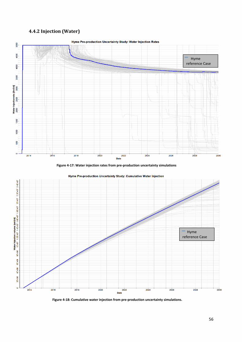
56
4.4.2 Injection (Water)
Hyme reference Case
Hyme reference Case
Figure 4-17: Water injection rates from pre-production uncertainty simulations
Figure 4-18: Cumulative water injection from pre-production uncertainty simulations.

57
4.4.3 Discussion concerning pre-production simulation results
In general, the Hyme reference case and the 130 pre-production uncertainty simulations
show general alignment. The reference case seems to be an average curve in each of the
plots (Figure 4-11 to Figure 4-18). For oil production rate (Figure 4-11) there are variations in
how long the production is on plateau rate of 2500 Sm3/d, with the following decline. This
are reflected in the cumulative oil production (Figure 4-12), which also has variations. Since
one of the main objectives in this thesis is to quantify the uncertainty ranges of the ultimate
estimated oil recovery, this will be studied more in detail in section 4.5.
As expected, the gas production rates (Figure 4-13) follows the same trend as the oil
production rates, since production most of the time are kept above the bubble point
pressure. This gives approximately the same variations in cumulative gas production (Figure
4-14) as for the cumulative oil production.
For water production rates (Figure 4-16) there are variations in the first 6 years of the
production, until the rate reaches the maximum water production rate constraint (Table
3-13) at 3500 Sm3/d. From this point, all the cases are producing water at the maximum rate.
This gives a cumulative water production with smaller variations compared with cumulative
oil and gas production.
All injection rates (Figure 4-17) starts on the maximum injection rate constraint (Table 3-13) of
5000 Sm3/d. There are some variations in terms of when injection rate are declining from
this rate. Some of the cases have a decline in injection earlier, and then builds up to the
constraint again. This can be explained by the fact that the injection is controlled by pressure
maintenance. Nevertheless, the injection rate is in general large for each case, which gives
high cumulative water injection (Figure 4-18) with small variations.
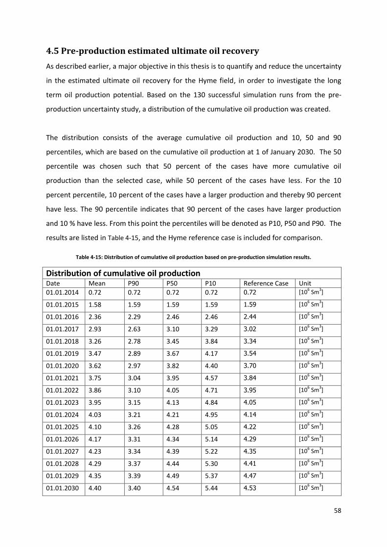
58
4.5 Pre-production estimated ultimate oil recovery
As described earlier, a major objective in this thesis is to quantify and reduce the uncertainty
in the estimated ultimate oil recovery for the Hyme field, in order to investigate the long
term oil production potential. Based on the 130 successful simulation runs from the pre-
production uncertainty study, a distribution of the cumulative oil production was created.
The distribution consists of the average cumulative oil production and 10, 50 and 90
percentiles, which are based on the cumulative oil production at 1 of January 2030. The 50
percentile was chosen such that 50 percent of the cases have more cumulative oil
production than the selected case, while 50 percent of the cases have less. For the 10
percent percentile, 10 percent of the cases have a larger production and thereby 90 percent
have less. The 90 percentile indicates that 90 percent of the cases have larger production
and 10 % have less. From this point the percentiles will be denoted as P10, P50 and P90. The
results are listed in Table 4-15, and the Hyme reference case is included for comparison.
Table 4-15: Distribution of cumulative oil production based on pre-production simulation results.
Distribution of cumulative oil production Date Mean P90 P50 P10 Reference Case Unit
01.01.2014 0.72 0.72 0.72 0.72 0.72 [106 Sm
3]
01.01.2015 1.58 1.59 1.59 1.59 1.59 [106 Sm
3]
01.01.2016 2.36 2.29 2.46 2.46 2.44 [106 Sm
3]
01.01.2017 2.93 2.63 3.10 3.29 3.02 [106 Sm
3]
01.01.2018 3.26 2.78 3.45 3.84 3.34 [106 Sm
3]
01.01.2019 3.47 2.89 3.67 4.17 3.54 [106 Sm
3]
01.01.2020 3.62 2.97 3.82 4.40 3.70 [106 Sm
3]
01.01.2021 3.75 3.04 3.95 4.57 3.84 [106 Sm
3]
01.01.2022 3.86 3.10 4.05 4.71 3.95 [106 Sm
3]
01.01.2023 3.95 3.15 4.13 4.84 4.05 [106 Sm
3]
01.01.2024 4.03 3.21 4.21 4.95 4.14 [106 Sm
3]
01.01.2025 4.10 3.26 4.28 5.05 4.22 [106 Sm
3]
01.01.2026 4.17 3.31 4.34 5.14 4.29 [106 Sm
3]
01.01.2027 4.23 3.34 4.39 5.22 4.35 [106 Sm
3]
01.01.2028 4.29 3.37 4.44 5.30 4.41 [106 Sm
3]
01.01.2029 4.35 3.39 4.49 5.37 4.47 [106 Sm
3]
01.01.2030 4.40 3.40 4.54 5.44 4.53 [106 Sm
3]
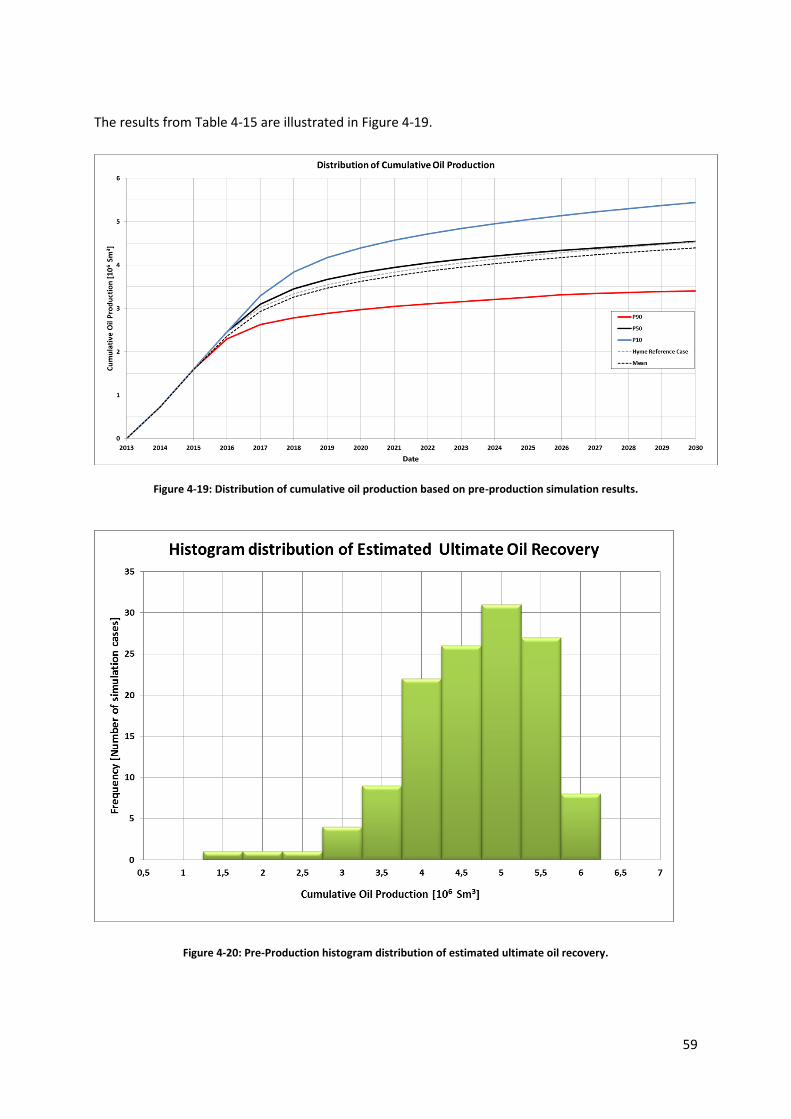
59
The results from Table 4-15 are illustrated in Figure 4-19.
Figure 4-19: Distribution of cumulative oil production based on pre-production simulation results.
Figure 4-20: Pre-Production histogram distribution of estimated ultimate oil recovery.

60
Figure 4-21: Pre-Production histogram versus cumulative distribution function
Based on the results from Table 4-15 and Figure 4-19, there are general alignment between
the Hyme reference case and the P50. The mean value is about 3% lower than the P50 which
mainly are related to the downside in in-place volumes. The estimated ultimate recovery is
considered as the total cumulative oil production at 1st of January 2030. The distribution of
the estimated ultimate oil recovery is illustrated by the histogram in Figure 4-20.
From Figure 4-20 it can be observed that the simulations resulted in an estimated ultimate oil
recovery range of 1.5 to 6 million Sm3. In order to capture the uncertainty range between
P90 and P10 within the histogram, a probability distribution histogram with a cumulative
distribution function was created (Figure 4-21). This was done by normalizing the frequency
to relative frequency. A cumulative distribution function was added in order to observe the
different percentiles within the histogram. The cumulative distribution function can be
defined as the cumulative relative frequency.
Based on the P90 and P10, which provides a 90% confidence interval, from Figure 4-19,
Figure 4-21 and Table 4-15 , the estimated ultimate oil recovery should be within the
uncertainty range of 3.40 to 5.44 million Sm3.
61
5. Post-production Uncertainty Study A post-production uncertainty study will be performed based on the Hyme reference case
established in chapter 3, sensitivity analysis performed in chapter and available production
data. The workflow is described in Figure 5-1.
5.0.1 History Matching
History matching can be defined as the process of adjusting parameters in a reservoir
simulation model until the simulated performance matches the measured performance
within an accepted tolerance (Caers, 2005). Alternatively, history matching can be defined as
the process of conditioning the reservoir model on dynamic, as well as static observations.
The aim of this process is to create reservoir models which have an improved prediction
power for prediction of future resources and reserves.
In traditional history matching, deterministic models are being considered, where properties
are changed in order to calibrate the model. These modified properties are parameters that
are considered uncertain (Almeida Netto et. al, 2003). This means that the engineer has to
manually change the selected parameters by the trial-and-error principle. Common
performance data to be matched are (Kleppe, 2010):
Reservoir Pressure; average pressure and pressure distributions.
Fluid movement, saturation from cores, tracer tests, arrival times for injected fluids
at producers.
Well observations; rates, pressures, water cut, gas oil ratio.
At the time this study was performed, 2 months of production was data available from the
Hyme field. These data were the oil production rates and bottom hole pressure data. As oil
production rate is at plateau rate during the 2 months period, it was decided that bottom
hole pressure is the key observation data that will be utilized in history matching for this
study.
Another less time consuming approach is to use computer assisted history matching
software instead of manual adjusting. Such software is integrated in the simulation
workflow, and allows the user to use an experimental design. Assisted history matching can

62
be defined as a process where the quality of a model is improved by gradually changing the
input variables such that the simulated output becomes closer to the observed production
data (Reis et al., 2009).
This study used the assisted history matching software Olyx developed by Resoptima. Olyx is
a plug-in used with Petrel and is designed for history matching and optimization of reservoir
simulation models. The software enables the user to integrate any kind of geological and
geophysical property as a variable in addition to more familiar reservoir engineering
variables (Resoptima, 2012). For this study, it is a great advantage that Olyx is a plug-in for
Petrel, as it allows keeping the same workflow as in pre-production study and therefore the
same experimental design.
5.0.2 Objective function
The procedure for performing a computer assisted history match has two major steps. The
first step is to define an objective function, which is defined as a mathematical expression
describing the difference between simulated and observed data. The next step will be
minimizing the objective function by using an optimization algorithm (Reis et al., 2009). Olyx
defines the objective function as
√∑
(
)
where
i is the objective element index
j is the observed sample point index
Qi is the objective function
mi is the multiplier of objective element i
Ni is the number of valid observed sample points for objective element i
Simi,j is the simulated value for objective element at observed point j
Obsi,j is the observed value for objective element I at observed point j
σ i ,j is the measurement error of objective element I at observed point j
As the only objective element of this study is bottom hole pressure, the objective element
index can be denoted with bhp. It will not be used any multipliers since all data points will be
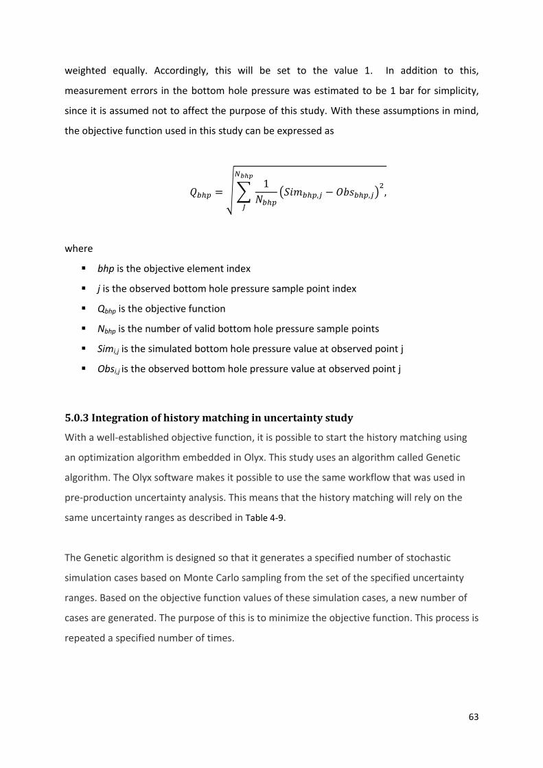
63
weighted equally. Accordingly, this will be set to the value 1. In addition to this,
measurement errors in the bottom hole pressure was estimated to be 1 bar for simplicity,
since it is assumed not to affect the purpose of this study. With these assumptions in mind,
the objective function used in this study can be expressed as
√∑
( )
where
bhp is the objective element index
j is the observed bottom hole pressure sample point index
Qbhp is the objective function
Nbhp is the number of valid bottom hole pressure sample points
Simi,j is the simulated bottom hole pressure value at observed point j
Obsi,j is the observed bottom hole pressure value at observed point j
5.0.3 Integration of history matching in uncertainty study
With a well-established objective function, it is possible to start the history matching using
an optimization algorithm embedded in Olyx. This study uses an algorithm called Genetic
algorithm. The Olyx software makes it possible to use the same workflow that was used in
pre-production uncertainty analysis. This means that the history matching will rely on the
same uncertainty ranges as described in Table 4-9.
The Genetic algorithm is designed so that it generates a specified number of stochastic
simulation cases based on Monte Carlo sampling from the set of the specified uncertainty
ranges. Based on the objective function values of these simulation cases, a new number of
cases are generated. The purpose of this is to minimize the objective function. This process is
repeated a specified number of times.

64
After all simulations are performed, each case will have an objective function value
associated with it. A traditional method is to use the model with the lowest objective
function value for further analysis. Another possibility is to set an upper limit to the objective
function so that all cases with lower value are analyzed further (Reis et al., 2009). The
advantage of this method is that the model is history matched in addition to the simulation
cases can be part of a post-production analysis, where the results can be treated statistically.
This methodology are used as described for this study, using the workflow in Figure 5-1 with
bottom hole pressure values listed in section 5.1.
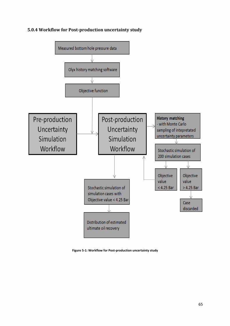
65
5.0.4 Workflow for Post-production uncertainty study
Figure 5-1: Workflow for Post-production uncertainty study
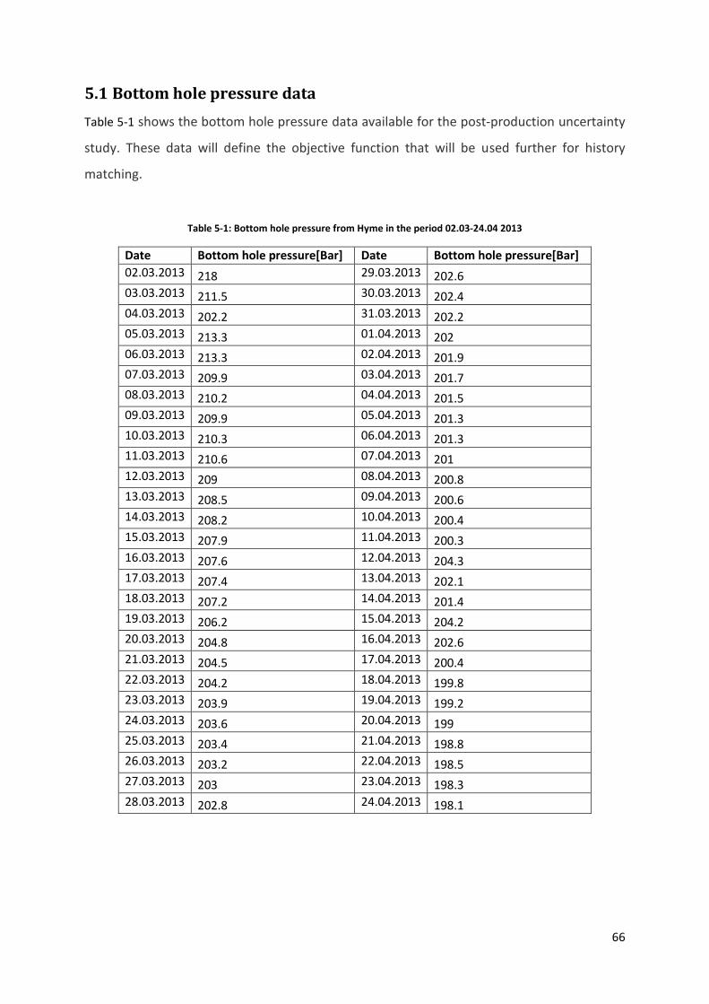
66
5.1 Bottom hole pressure data
Table 5-1 shows the bottom hole pressure data available for the post-production uncertainty
study. These data will define the objective function that will be used further for history
matching.
Table 5-1: Bottom hole pressure from Hyme in the period 02.03-24.04 2013
Date Bottom hole pressure[Bar] Date Bottom hole pressure[Bar]
02.03.2013 218 29.03.2013 202.6
03.03.2013 211.5 30.03.2013 202.4
04.03.2013 202.2 31.03.2013 202.2
05.03.2013 213.3 01.04.2013 202
06.03.2013 213.3 02.04.2013 201.9
07.03.2013 209.9 03.04.2013 201.7
08.03.2013 210.2 04.04.2013 201.5
09.03.2013 209.9 05.04.2013 201.3
10.03.2013 210.3 06.04.2013 201.3
11.03.2013 210.6 07.04.2013 201
12.03.2013 209 08.04.2013 200.8
13.03.2013 208.5 09.04.2013 200.6
14.03.2013 208.2 10.04.2013 200.4
15.03.2013 207.9 11.04.2013 200.3
16.03.2013 207.6 12.04.2013 204.3
17.03.2013 207.4 13.04.2013 202.1
18.03.2013 207.2 14.04.2013 201.4
19.03.2013 206.2 15.04.2013 204.2
20.03.2013 204.8 16.04.2013 202.6
21.03.2013 204.5 17.04.2013 200.4
22.03.2013 204.2 18.04.2013 199.8
23.03.2013 203.9 19.04.2013 199.2
24.03.2013 203.6 20.04.2013 199
25.03.2013 203.4 21.04.2013 198.8
26.03.2013 203.2 22.04.2013 198.5
27.03.2013 203 23.04.2013 198.3
28.03.2013 202.8 24.04.2013 198.1

67
5.1.1 Determination of objective value criteria for history matching
Based on the measured values of the bottom hole pressure in Table 5-1 and the simulation
results from Hyme reference case, an objective value criteria for history matching was
determined. The objective value for Hyme reference case was calculated by Olyx to be 4.25
bar. This value can be considered as a good match, which can be observed in Figure 5-2.
Figure 5-2: Measured bottom hole pressure compared with Hyme reference case where day 0 is April 2 2013.
Since the reference case turned out to be a god match with the observed data, the criteria
was determined to be every objective value less 4.25 bar. This means that out of the 230
simulated cases, all cases with an objective value less than 4.25 bar will be included in the
post-production uncertainty analysis.

68
5.2 Post-production uncertainty analysis results
There was in total 50 cases that complement the objective function value of less than 4.25
bar, which makes the basis for the results of the post-production uncertainty study. The
study is divided into three parts, where the first part consists of the uncertainty ranges for
the input parameters to the post-production study. The second part consist plots of the
stochastic simulation results, and the second part shows the statistical treatment of the
simulation results for cumulative oil production, in alignment with chapter 4.
5.3 Post-production uncertainty input parameters
After the history matching process was performed, 50 cases matched the preset criteria.
These cases were generated by Monte Carlo sampling from the same table as for the pre-
production study (Table 4-9). Based on the 50 cases it was possible to create new ranges for
the uncertainty input, based on maximum and minimum values for each of the sampled
parameters. For the discrete input, the percentage was calculated based on appearance
relative to number of cases included. The uncertainty input ranges are listed in Table 5-2.
Table 5-2: Ranges for post-production uncertainty input parameters
Uncertainty Low Reference High Description
Pore volume eastern segment 0.66 1 1.55 Multiplier
Pore volume western segment 0.49 1 1.36 Multiplier
Horizontal Permeability 0.32 1 3.46 Multiplier
Vertical Permeability 0.01 0.1 0.5 Multiplier
Transmissibility multiplier Z1 0 0 0.1 Multiplier
Transmissibility multiplier Z2 0 0 0.1 Multiplier
Transmissibility multiplier Z3 0 0.0001 0.1 Multiplier
Transmissibility multiplier Z4 0 0 0.1 Multiplier
Relative permeability 22 % (oil-wet) 40 % (mixed wet) 28 % (water-wet) Discrete
Fault seal 20 % (tight) 40 % (reference) 40 % (open) Discrete
From Table 5-2 it can be observed that some of the ranges are smaller compared with Table
4-9, which will be discussed more in chapter 6. For faults, the reference and high case
suggest communications, which implies that 80 % of the cases included in this study, had
communication.
69
5.4 Post-production simulation results
Out of the 230 simulation cases generated by through the workflow, 50 cases had an
objective function value less than 4.25 bar. These cases were run to 1st of January 2030 in
alignment with the pre-production study. The raw simulation results for the 50 cases are
organized in plots and they are compared with the Hyme reference case. Simulation results
are displayed with a grey color, while the Hyme reference case has an actual color in
alignment with the pre-production study.
Oil production is displayed in Figure 5-3 and Figure 5-4 with the Hyme reference case in green.
It can be observed from the oil production rates (Figure 5-3) that the variations in how long
the production is on the plateau rate of 2500 Sm3/d, are less compared with the pre-
production study. This affects the cumulative oil production (Figure 5-4) where the spread in
the results looks smaller compared with pre-production study. The reference case seems to
be in the middle; however there is a larger density of cases above it, implying potential for
higher oil rate. The same trends can be observed in gas production (Figure 5-5 and Figure 5-6)
where the reference case is illustrated with red.
Water production is displayed in Figure 5-7 and Figure 5-8 with the Hyme reference case in
blue. The water rates (Figure 5-7) still reaches the production constraint of 3500 Sm3/d
within few years resulting in small variations in cumulative water production (Figure 5-8).
However there is less spread in the water rates and a larger density of cases with less water
production compared with the pre-production study.
Water injection is illustrated in Figure 5-9 and Figure 5-10 with the Hyme reference case in
blue. The results for water injection are very similar to the pre-production study, but the
spreading are diminished, both injection rates and hence cumulative injection.
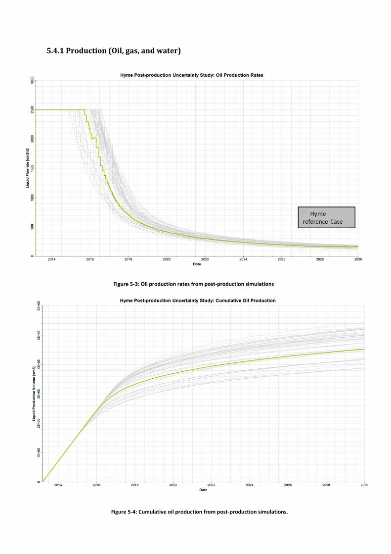
70
5.4.1 Production (Oil, gas, and water)
Figure 5-3: Oil production rates from post-production simulations
Figure 5-4: Cumulative oil production from post-production simulations.
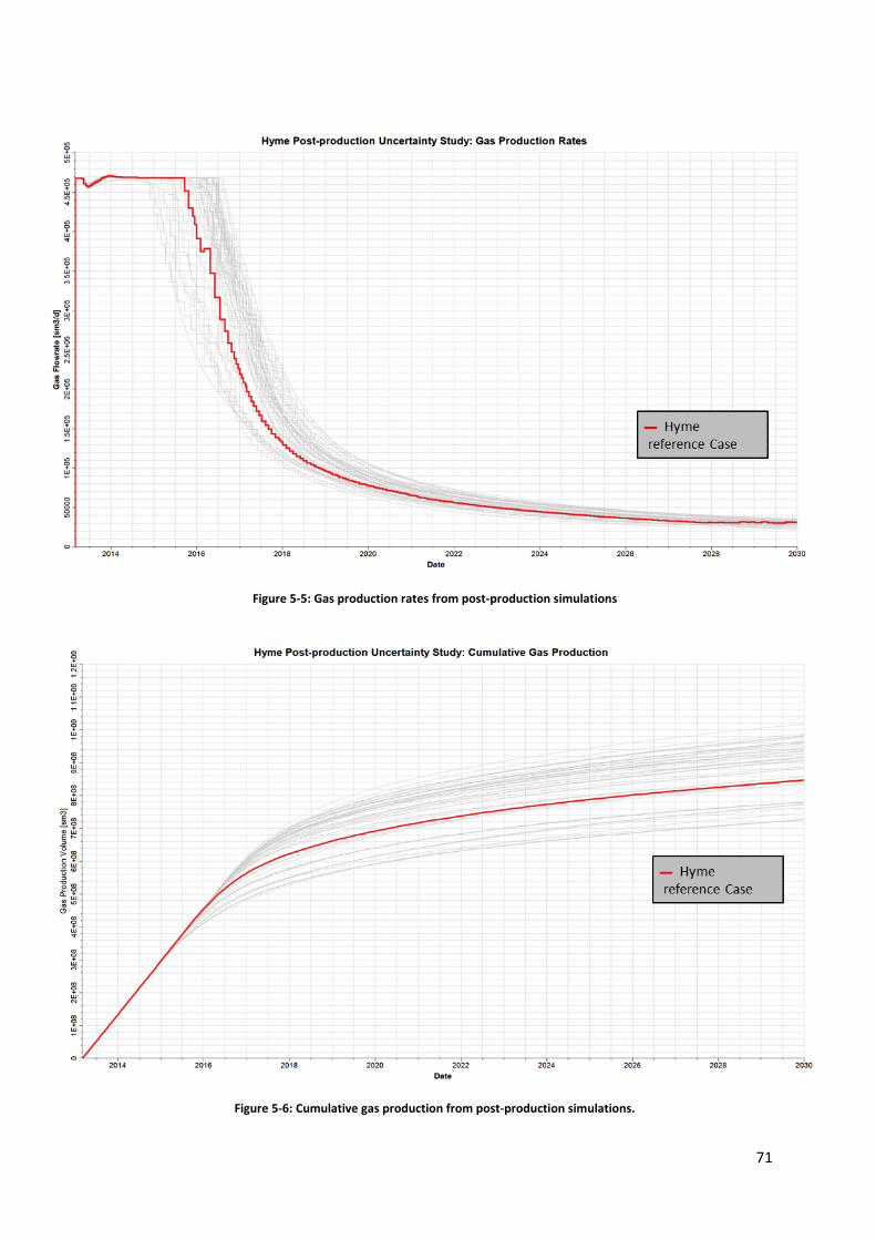
71
Figure 5-5: Gas production rates from post-production simulations
Figure 5-6: Cumulative gas production from post-production simulations.
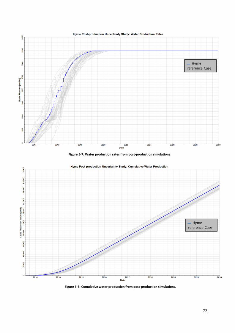
72
Figure 5-7: Water production rates from post-production simulations
Figure 5-8: Cumulative water production from post-production simulations.

73
5.4.2 Injection (Water)
Figure 5-9: Water injection rates from post-production simulations
Figure 5-10: Cumulative water injection from post-production simulations.

74
5.5 Post-production estimated ultimate oil recovery
The post-production results were treated statistically in alignment with the pre-production
study. Based on the 50 simulation cases with an objective value lower than 4.25 bar, a
distribution of the cumulative oil production was created.
The distribution consists of the average cumulative oil production, P10, P50 and P90 which
are based on the cumulative oil production at 1st of January 2030. The percentiles were
determined in the same way as for the pre-production uncertainty study (Section 4.5). Hyme
reference case is also included for comparison, and the results are listed in Table 5-3 .
Table 5-3: Distribution of cumulative oil production based on post-production simulation results
Distribution of cumulative oil production Date Mean P90 P50 P10 Reference Case Unit
01.01.2014 0.72 0.72 0.72 0.72 0.72 [106 Sm
3]
01.01.2015 1.59 1.59 1.59 1.59 1.59 [106 Sm
3]
01.01.2016 2.42 2.23 2.45 2.46 2.44 [106 Sm
3]
01.01.2017 3.06 2.60 3.11 3.24 3.02 [106 Sm
3]
01.01.2018 3.44 2.85 3.47 3.70 3.34 [106 Sm
3]
01.01.2019 3.67 3.03 3.67 3.99 3.54 [106 Sm
3]
01.01.2020 3.84 3.19 3.82 4.21 3.70 [106 Sm
3]
01.01.2021 3.98 3.31 3.94 4.38 3.84 [106 Sm
3]
01.01.2022 4.10 3.43 4.04 4.53 3.95 [106 Sm
3]
01.01.2023 4.20 3.52 4.13 4.66 4.05 [106 Sm
3]
01.01.2024 4.29 3.61 4.21 4.76 4.14 [106 Sm
3]
01.01.2025 4.38 3.69 4.28 4.86 4.22 [106 Sm
3]
01.01.2026 4.45 3.77 4.35 4.94 4.29 [106 Sm
3]
01.01.2027 4.52 3.83 4.41 5.02 4.35 [106 Sm
3]
01.01.2028 4.58 390 4.47 5.09 4.41 [106 Sm
3]
01.01.2029 4.64 3.96 4.53 5.15 4.47 [106 Sm
3]
01.01.2030 4.70 4.01 4.59 5.21 4.53 [106 Sm
3]
The results from Table 5-3 are illustrated in Figure 5-11. There are general alignment with
P50 and Hyme reference case; however the mean is significantly higher. This is mainly due to
larger density of cases with higher oil production which was observed in section 5.2. The
distribution of the estimated ultimate oil recovery is illustrated by the histogram in Figure
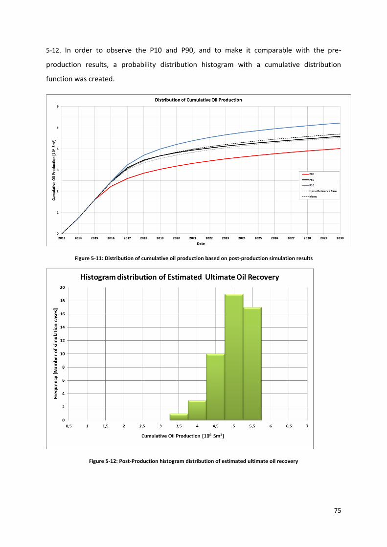
75
5-12. In order to observe the P10 and P90, and to make it comparable with the pre-
production results, a probability distribution histogram with a cumulative distribution
function was created.
Figure 5-11: Distribution of cumulative oil production based on post-production simulation results
Figure 5-12: Post-Production histogram distribution of estimated ultimate oil recovery
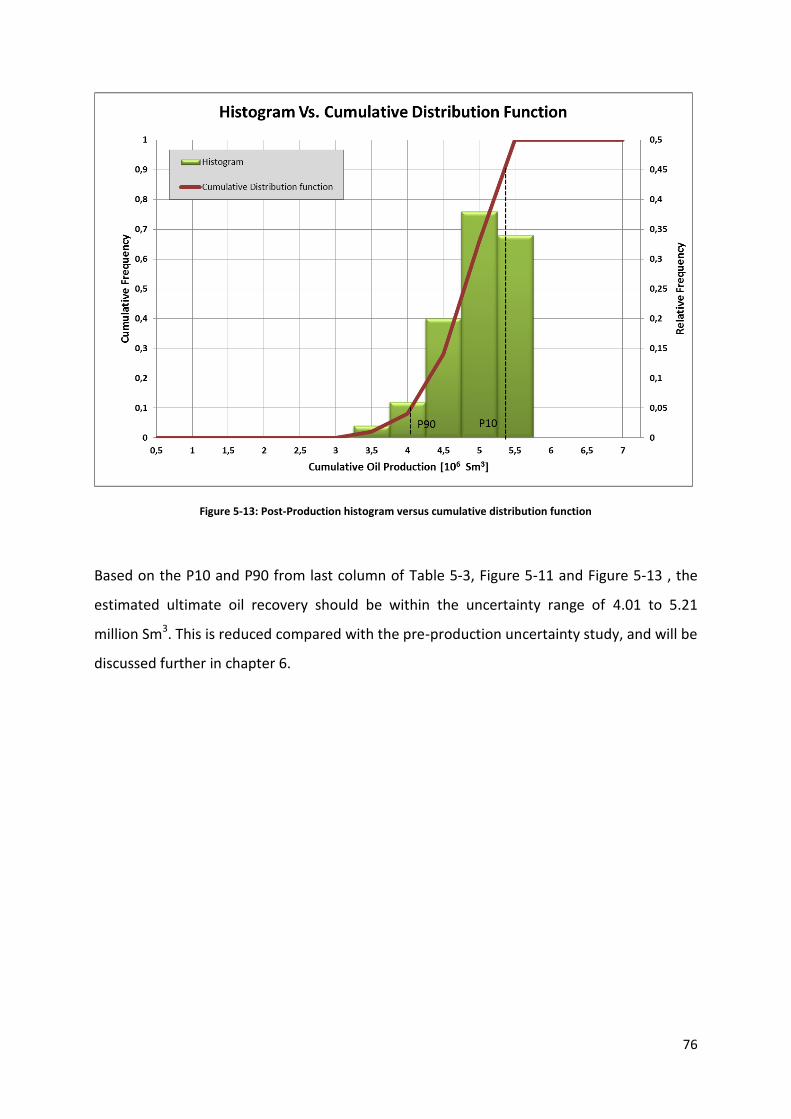
76
Figure 5-13: Post-Production histogram versus cumulative distribution function
Based on the P10 and P90 from last column of Table 5-3, Figure 5-11 and Figure 5-13 , the
estimated ultimate oil recovery should be within the uncertainty range of 4.01 to 5.21
million Sm3. This is reduced compared with the pre-production uncertainty study, and will be
discussed further in chapter 6.

77
6. Pre/post-production uncertainty discussion
The sensitivity results in section 4.3 stated that the pore volume multipliers were the
parameters that affected oil volume in-place and cumulative oil production the most. In
addition to this, the horizontal permeability and relative permeability had significant effect.
From the pre-production to the post-production results, the uncertainty in these parameters
is reduced, which can be observed on the deltas in Table 6-1 and Table 6-2.
Table 6-1: Comparison of pre/post-production low case input parameters
Uncertainty Low case
Pre Post Delta Description
Pore volume eastern segment 0.50 0.66 0.16 Multiplier
Pore volume western segment 0.20 0.49 0.29 Multiplier
Horizontal Permeability 0.20 0.32 0.12 Multiplier
Vertical Permeability 0.01 0.01 0 Multiplier
Transmissibility multiplier Z1 0 0 0 Multiplier
Transmissibility multiplier Z2 0 0 0 Multiplier
Transmissibility multiplier Z3 0 0 0 Multiplier
Transmissibility multiplier Z4 0 0 0 Multiplier
Relative permeability 30 % 22 % 8 % Discrete
Fault seal 30 % 20 % 10 % Discrete
Table 6-1 shows a comparison between the pre and post-production low case input
parameters. It can be observed that the deltas between the pore volume multipliers are
large, especially for the western segment with a delta of 0.29. The uncertainty in horizontal
permeability is also reduced, implied by the delta of 0.12. For the transmissibility multipliers
there are no changes, which can be explained by that the ranges were small initially.
For the discrete input parameters it can be observed the relative frequency of low case
relative permeability and sealed fault are less in the post-production study compared with
the pre-production study. This can imply that the probability of an oil wet reservoir and a
sealed fault are less than initially expected.
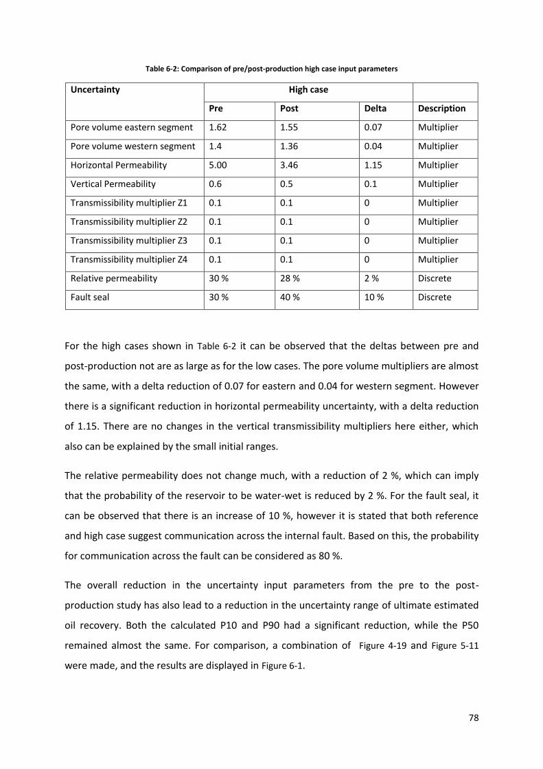
78
Table 6-2: Comparison of pre/post-production high case input parameters
Uncertainty High case
Pre Post Delta Description
Pore volume eastern segment 1.62 1.55 0.07 Multiplier
Pore volume western segment 1.4 1.36 0.04 Multiplier
Horizontal Permeability 5.00 3.46 1.15 Multiplier
Vertical Permeability 0.6 0.5 0.1 Multiplier
Transmissibility multiplier Z1 0.1 0.1 0 Multiplier
Transmissibility multiplier Z2 0.1 0.1 0 Multiplier
Transmissibility multiplier Z3 0.1 0.1 0 Multiplier
Transmissibility multiplier Z4 0.1 0.1 0 Multiplier
Relative permeability 30 % 28 % 2 % Discrete
Fault seal 30 % 40 % 10 % Discrete
For the high cases shown in Table 6-2 it can be observed that the deltas between pre and
post-production not are as large as for the low cases. The pore volume multipliers are almost
the same, with a delta reduction of 0.07 for eastern and 0.04 for western segment. However
there is a significant reduction in horizontal permeability uncertainty, with a delta reduction
of 1.15. There are no changes in the vertical transmissibility multipliers here either, which
also can be explained by the small initial ranges.
The relative permeability does not change much, with a reduction of 2 %, which can imply
that the probability of the reservoir to be water-wet is reduced by 2 %. For the fault seal, it
can be observed that there is an increase of 10 %, however it is stated that both reference
and high case suggest communication across the internal fault. Based on this, the probability
for communication across the fault can be considered as 80 %.
The overall reduction in the uncertainty input parameters from the pre to the post-
production study has also lead to a reduction in the uncertainty range of ultimate estimated
oil recovery. Both the calculated P10 and P90 had a significant reduction, while the P50
remained almost the same. For comparison, a combination of Figure 4-19 and Figure 5-11
were made, and the results are displayed in Figure 6-1.
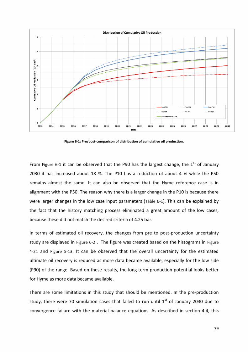
79
Figure 6-1: Pre/post-comparison of distribution of cumulative oil production.
From Figure 6-1 it can be observed that the P90 has the largest change, the 1st of January
2030 it has increased about 18 %. The P10 has a reduction of about 4 % while the P50
remains almost the same. It can also be observed that the Hyme reference case is in
alignment with the P50. The reason why there is a larger change in the P10 is because there
were larger changes in the low case input parameters (Table 6-1). This can be explained by
the fact that the history matching process eliminated a great amount of the low cases,
because these did not match the desired criteria of 4.25 bar.
In terms of estimated oil recovery, the changes from pre to post-production uncertainty
study are displayed in Figure 6-2 . The figure was created based on the histograms in Figure
4-21 and Figure 5-13. It can be observed that the overall uncertainty for the estimated
ultimate oil recovery is reduced as more data became available, especially for the low side
(P90) of the range. Based on these results, the long term production potential looks better
for Hyme as more data became available.
There are some limitations in this study that should be mentioned. In the pre-production
study, there were 70 simulation cases that failed to run until 1st of January 2030 due to
convergence failure with the material balance equations. As described in section 4.4, this
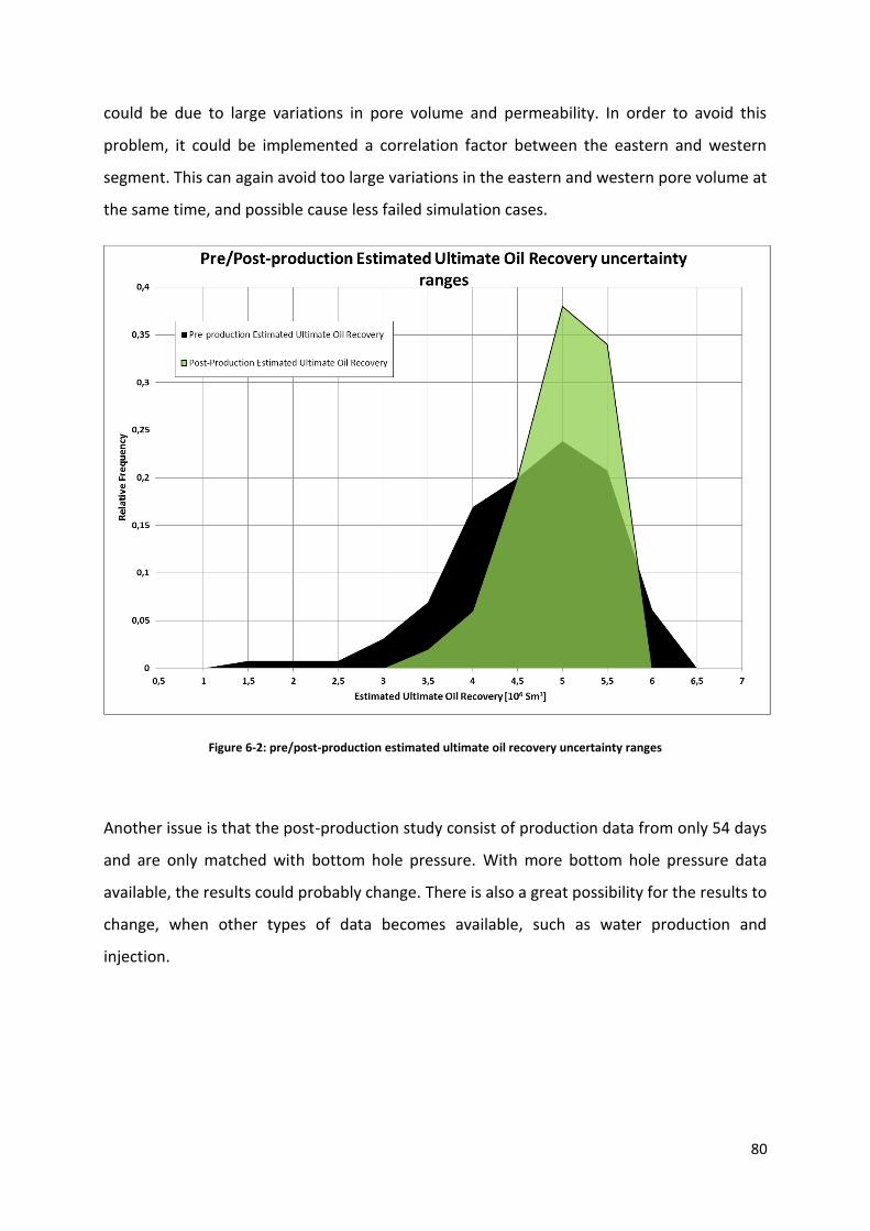
80
could be due to large variations in pore volume and permeability. In order to avoid this
problem, it could be implemented a correlation factor between the eastern and western
segment. This can again avoid too large variations in the eastern and western pore volume at
the same time, and possible cause less failed simulation cases.
Figure 6-2: pre/post-production estimated ultimate oil recovery uncertainty ranges
Another issue is that the post-production study consist of production data from only 54 days
and are only matched with bottom hole pressure. With more bottom hole pressure data
available, the results could probably change. There is also a great possibility for the results to
change, when other types of data becomes available, such as water production and
injection.

81
7. Conclusions
A pre/post production uncertainty study was performed on the Hyme field in order to
quantify how predicted uncertainty will change as more data becomes available. This was
done by first performing a pre-production uncertainty study based on stochastic simulations
with Monte Carlo sampling from interpreted uncertainty ranges for input parameters.
Secondly, the study was performed again by including actual production data in a history
matching process. Results from these studies was treated statistically, and compared in
terms of the uncertainty ranges of the ultimate estimated oil recovery.
The results from the pre-production uncertainty study indicated that the pore volume
multipliers are the most sensitive parameters. These parameters had a deep impact on both
oil volumes in-place and the cumulative oil production. Additionally, the horizontal
permeability and relative permeability also have a significant impact on the cumulative oil
production.
Based on the results from both pre and post-production studies, it can be concluded that the
uncertainty ranges for the pore volume multipliers have been reduced, especially on the low
side. The uncertainty range was also reduced for the horizontal permeability. For the relative
permeability it can be concluded that the probability for an oil-wet reservoir has been
reduced. In addition to this, it can be concluded that there is 80 % probability for
communication across the internal fault.
Results for the pre/post-uncertainty study have led to a significant reduction in the
uncertainty range of the estimated ultimate oil recovery. A conclusion that can be drawn
from this is that there is less uncertainty, hence a lower risk in the Hyme long term
production potential as more data becomes available.
The model and workflow used in this thesis has been constructed, tested and is ready for use
as a tool for VNG in future evaluation of Hyme. For the future, it is recommended to include
more bottom hole pressure data and integration of other production data as they become
available.
82
8. References
Almeida Netto, S.L, Schiozer, D.J., Ligero, E.L. and Maschio, C.: “History Matching
using Uncertainty Analysis” Canadian International Petroleum Conference, Jun 10 -
12, 2003, Calgary, Alberta
Archie, G.E.: “The electrical resistivity log as an aid in determining some reservoir
characteristics” Petroleum Transactions of AIME (January 1942) pp.54-62.
Breitenbach, E.A.: “Reservoir Simulation: State of the Art”, JPT(September 1991), pp.
1033- 1036
Caers, J.: “Petroleum Geostatics”, 2005, SPE, ISBN 978-1-55583-106-2, pp. 53-63
Dalland, A., Worsley, D. and Ofstad, K. 1988: “A lithostratigrafic scheme for the
Mesozoic and Cenozoic succession offshore mid- and northern Norway”, NPD-
bulletin No 4 (January 1988), pp.10-12.
Damsleth, E., Hage, A. and Volden,R.: “Maximum Information at Minimum Cost: A
North Sea Field Development Study With an Experimental Design”, JPT( November
1992, Vol.44, No 12, pp. 1350-1356
Haldorsen, H.H. and Damsleth, E.: “Stochastic modeling”, JPT(April 1990), pp.404-412
Kleppe, H.:”Notes RESERVOIR SIMULATION”, University of Stavanger (2010), pp. 1-39
and pp.112-114
Lehne, K.A.:”Geologisk brønnlogging”, 1985, Universitetsforlaget AS, ISBN 82-00-
06875-7, pp. 17-50
Lépine, O.J., Bissell, R.C., Aanonsen, S.I., Pallister, I.C. and Barker, J.W.: ”Uncertainty
in Predictive Reservoir simulation using gradient information” SPE Journal, Vol. 4, No
3 (September 1999), pp.251-259
Li-Bong, W.L., Krum, G.L., Yao, T., Wattenbarger, R.C. and Landis, L.H.: Application of
Model-Based Uncertainty Analysis” , Abu Dhabi International Petroleum Exhibition
and Conference, 5-8 November 2006, Abu Dhabi, UAE, pp.1-5
Lisboa, E. and Duarte, R.: “Uncertainty Analysis Considering the Production History:
Evaluation of a Real Field”, SPE Latin American and Caribbean Petroleum Engineering
Confrence, 1-3 December 2010, Lima, Peru, pp. 1-10
83
Martinius, A.W., Ringrose, P.S., Næss, A., Wen, R.: “Multi-Scale Characterization and
Modeling of Heterolithic Tidal Systems, Offshore Mid-Norway”, 1999. In: "Advanced
Reservoir Characterization for the 21st Century" Hentz, T. F. (ed), Proceedings of
GCSSEPM Research Conference, pp. 193-204. Houston, U.S.A, (December 5-8, 1999)
Mattax, C.C and Dalton, R.L.: “Reservoir Simulation” , JPT (June 1990), pp. 692-695
Reid, B.E., Høyland, L.A., Olsen S.R. and Petterson, O.: “The Heidrun Field –
Challenges in Reservoir Development and Production”, OTC (May 1996), pp.521-534
Reis, L.C, dos Reis, L.E, da Silva, L.C. and Becerra, G.G.: “History Matching: Is it
Necessary to Optimize?”, Latin American and Caribbean Petroleum Engineering
Conference, 31 May -3 June 2009, Cartagena de Indias, Colombia, pp. 1-11
Resoptima: “ Olyx User guide”, 2012, version 1.3.0
Schlumberger:”Petrel Help Manual”, 2012
Skjaeveland, S.M., Siqveland, L.M., Kjosavik, A., Hammervold Thomas, W.L. and
Virnovsky, G.A.: "Capillary Pressure Correlation for Mixed-Wet Reservoirs" SPE
Reservoir Eval. & Eng., Vol. 3, No 1 (February 2000), pp. 60-67
Statoil: “Book 201 Petroleum Technology Report - Hyme Project DG3”, 2012, pp. 1-
274
Steagall, D.E and Schiozer, D.J.: “Uncertainty Analysis In Reservoir Production
Forecast During Apraisal And Piliot Production Phases”, SPE 66399 (February 2001),
pp.1-8
Stoian, E.: ”Fundamentals and Applications of the Monte Carlo Method”, Journal of
Canadian Petroleum, Vol. 4, No 1 (July-September 1965), pp.120-129
Walstrom, J.E., Mueller, T.D. and McFarline, R.C.: “Evaluating Uncertainty in
Engineering Calculations” , JPT(December 1967), Vol. 19, No 12, pp. 1595-1603

84
9. Appendix A
Hyme Reference case: – Eclipse 100 simulation deck This section is a copy of the Eclipse 100 simulation deck of the Hyme reference case. The
main deck has several include files, and many of them are too long to be included in this
paper. Include files from props and schedule sections are included
RUNSPEC
MESSAGES
3* 15 /
TRACERS
1* 1 /
WSEGDIMS
1 264 2 /
VFPIDIMS
15 10 3 /
EQLDIMS
8 /
ENDSCALE
/
WPOTCALC
no /
TITLE
Hyme Reference Case
WELLDIMS
2 246 3 2 6* 3 /
START
2 MAR 2013 /
VAPOIL
DISGAS
WATER
OIL

85
GAS
GRIDOPTS
NO 8 /
PETOPTS
INITNNC /
MONITOR
MULTOUT
METRIC
DIMENS
77 114 156 /
TABDIMS
2 3 42 1* 8 7* 1 /
REGDIMS
8 2 /
NSTACK
200 /
NUPCOL
15 /
GRID
INCLUDE
'MB_REFERENCE_GRID.INC' /
NOECHO
GDFILE
MB_REFERENCE_GRID.EGRID /
INCLUDE
'MB_REFERENCE_PROP_PERMX.GRDECL' /
INCLUDE
'MB_REFERENCE_PROP_PERMY.GRDECL' /
INCLUDE
'MB_REFERENCE_PROP_PERMZ.GRDECL' /

86
INCLUDE
'MB_REFERENCE_PROP_NTG.GRDECL' /
INCLUDE
'MB_REFERENCE_PROP_PORO.GRDECL' /
INCLUDE
'MB_REFERENCE_PROP_ACTNUM.GRDECL' /
INCLUDE
'MB_REFERENCE_PROP_MULTNUM.GRDECL' /
ECHO
EDIT
INCLUDE
'MB_REFERENCE_EDIT.INC' /
PROPS
INCLUDE
'MB_REFERENCE_PROPS.INC' /
REGIONS
NOECHO
NCLUDE
'MB_REFERENCE_PROP_SATNUM.GRDECL' /
INCLUDE
'MB_REFERENCE_PROP_PVTNUM.GRDECL' /
INCLUDE
'MB_REFERENCE_PROP_ROCKNUM.GRDECL' /
INCLUDE
'MB_REFERENCE_PROP_EQLNUM.GRDECL' /
INCLUDE
'MB_REFERENCE_PROP_FIPNUM.GRDECL' /
INCLUDE
'MB_REFERENCE_PROP_FIPFAULT.GRDECL' /
ECHO

87
SOLUTION
INCLUDE
'MB_REFERENCE_SOL.INC' /
SUMMARY
INCLUDE
'MB_REFERENCE_SUM.INC' /
SCHEDULE
INCLUDE
'MB_REFERENCE_SCH.INC' /

88
'MB_REFERENCE_PROPS.INC' /
SCALECRS
YES/
TRACER
TR1 WAT /
/
ROCKOPTS
1* 1* ROCKNUM /
ROCK
216.8 7.833E-005 /
PVTW
198.2 1.0303 3.9868E-005 0.33034 8.9588E-005 /
198.2 1.0303 3.9868E-005 0.33034 8.9588E-005 /
198.2 1.0303 3.9868E-005 0.33034 8.9588E-005 /
PVTO
17.2 20 1.1152 0.574
50 1.1098 0.612
100 1.1019 0.678
150 1.0949 0.746
198.2 1.0889 0.812
250 1.0831 0.883
300 1.0781 0.951
350 1.0736 1.019
400 1.0694 1.086
450 1.0656 1.152
500 1.0621 1.217
550 1.0588 1.281
600 1.0558 1.345 /
45.8 50 1.214 0.456
89
100 1.2024 0.501
150 1.1925 0.548
198.2 1.1841 0.594
250 1.1761 0.644
300 1.1693 0.693
350 1.1631 0.742
400 1.1575 0.79
450 1.1524 0.838
500 1.1477 0.886
550 1.1434 0.933
600 1.1394 0.979 /
89.5 100 1.3482 0.336
150 1.3325 0.361
198.2 1.3196 0.385
250 1.3076 0.41
300 1.2974 0.435
350 1.2884 0.458
400 1.2804 0.482
450 1.273 0.505
500 1.2664 0.528
550 1.2603 0.55
600 1.2547 0.572 /
135.4 150 1.4804 0.264
198.2 1.4611 0.281
250 1.4437 0.299
300 1.4291 0.317
350 1.4164 0.333
400 1.4052 0.35
450 1.3951 0.366
500 1.3861 0.381

90
550 1.3778 0.397
600 1.3703 0.411 /
187.3 198.2 1.6288 0.214
250 1.6033 0.228
300 1.5825 0.241
350 1.5647 0.254
400 1.5491 0.266
450 1.5354 0.278
500 1.5231 0.29
550 1.5121 0.302
600 1.5021 0.313 /
/
17.2 20 1.1152 0.574
50 1.1098 0.612
100 1.1019 0.678
150 1.0949 0.746
198.2 1.0889 0.812
250 1.0831 0.883
300 1.0781 0.951
350 1.0736 1.019
400 1.0694 1.086
450 1.0656 1.152
500 1.0621 1.217
550 1.0588 1.281
600 1.0558 1.345 /
45.8 50 1.214 0.456
100 1.2024 0.501
150 1.1925 0.548
198.2 1.1841 0.594
250 1.1761 0.644
91
300 1.1693 0.693
350 1.1631 0.742
400 1.1575 0.79
450 1.1524 0.838
500 1.1477 0.886
550 1.1434 0.933
600 1.1394 0.979 /
89.5 100 1.3482 0.336
150 1.3325 0.361
198.2 1.3196 0.385
250 1.3076 0.41
300 1.2974 0.435
350 1.2884 0.458
400 1.2804 0.482
450 1.273 0.505
500 1.2664 0.528
550 1.2603 0.55
600 1.2547 0.572 /
135.4 150 1.4804 0.264
198.2 1.4611 0.281
250 1.4437 0.299
300 1.4291 0.317
350 1.4164 0.333
400 1.4052 0.35
450 1.3951 0.366
500 1.3861 0.381
550 1.3778 0.397
600 1.3703 0.411 /
187.3 198.2 1.6288 0.214
250 1.6033 0.228

92
300 1.5825 0.241
350 1.5647 0.254
400 1.5491 0.266
450 1.5354 0.278
500 1.5231 0.29
550 1.5121 0.302
600 1.5021 0.313 /
/
17.2 20 1.1152 0.574
50 1.1098 0.612
100 1.1019 0.678
150 1.0949 0.746
198.2 1.0889 0.812
250 1.0831 0.883
300 1.0781 0.951
350 1.0736 1.019
400 1.0694 1.086
450 1.0656 1.152
500 1.0621 1.217
550 1.0588 1.281
600 1.0558 1.345 /
45.8 50 1.214 0.456
100 1.2024 0.501
150 1.1925 0.548
198.2 1.1841 0.594
250 1.1761 0.644
300 1.1693 0.693
350 1.1631 0.742
400 1.1575 0.79
450 1.1524 0.838

93
500 1.1477 0.886
550 1.1434 0.933
600 1.1394 0.979 /
89.5 100 1.3482 0.336
150 1.3325 0.361
198.2 1.3196 0.385
250 1.3076 0.41
300 1.2974 0.435
350 1.2884 0.458
400 1.2804 0.482
450 1.273 0.505
500 1.2664 0.528
550 1.2603 0.55
600 1.2547 0.572 /
135.4 150 1.4804 0.264
198.2 1.4611 0.281
250 1.4437 0.299
300 1.4291 0.317
350 1.4164 0.333
400 1.4052 0.35
450 1.3951 0.366
500 1.3861 0.381
550 1.3778 0.397
600 1.3703 0.411 /
187.3 198.2 1.6288 0.214
250 1.6033 0.228
300 1.5825 0.241
350 1.5647 0.254
400 1.5491 0.266
450 1.5354 0.278

94
500 1.5231 0.29
550 1.5121 0.302
600 1.5021 0.313 /
/
PVTG
20 0.00001308 0.062612 0.013107
0.00001307 0.063071 0.013145 /
50 0.00001309 0.023645 0.014157
0.00001307 0.063323 0.013385 /
100 0.00002551 0.011215 0.016177
0.00001307 0.011241 0.013403 /
150 0.00007430 0.007312 0.019292
0.00001307 0.023922 0.013399 /
198.2 0.00017392 0.00559 0.024293
0.00001307 0.063339 0.013399 /
/
20 0.00001308 0.062612 0.013107
0.00001307 0.063071 0.013145 /
50 0.00001309 0.023645 0.014157

95
0.00001307 0.063323 0.013385 /
100 0.00002551 0.011215 0.016177
0.00001307 0.011241 0.013403 /
150 0.00007430 0.007312 0.019292
0.00001307 0.023922 0.013399 /
198.2 0.00017392 0.00559 0.024293
0.00001307 0.063339 0.013399 /
/
DENSITY
815.4 1028.1 1.1042 /
815.4 1028.1 1.1042 /
815.4 1028.1 1.1042 /
INCLUDE
'MB_REFERENCE_PROP_PROPS.GRDECL' /
FILLEPS
SWOF
0 0 1 0.0001
0.02075 1E-006 0.89232 9.5E-005
0.0415 1.3E-005 0.79388 9.025E-005
0.06225 5.2E-005 0.70411 8.5738E-005
0.083 0.000142 0.62243 8.1451E-005
0.10375 0.000311 0.54832 7.7378E-005
0.1245 0.000588 0.48127 7.3509E-005
0.14525 0.001009 0.42077 6.9834E-005
0.166 0.00161 0.36636 6.6342E-005
0.18675 0.002431 0.31758 6.3025E-005
0.2075 0.003516 0.27402 5.9874E-005
0.22825 0.004908 0.23525 5.688E-005
0.249 0.006655 0.20088 5.4036E-005
0.26975 0.008807 0.17056 5.1334E-005

96
0.2905 0.011414 0.14392 4.8767E-005
0.31125 0.014532 0.12063 4.6329E-005
0.332 0.018215 0.10039 4.4013E-005
0.35275 0.02252 0.082891 4.1812E-005
0.3735 0.027508 0.067863 3.9721E-005
0.39425 0.033238 0.055045 3.7735E-005
0.415 0.039775 0.044194 3.5849E-005
0.43575 0.047181 0.035085 3.4056E-005
0.4565 0.055524 0.027508 3.2353E-005
0.47725 0.064871 0.021269 3.0736E-005
0.498 0.075291 0.016191 2.9199E-005
0.51875 0.086855 0.01211 2.7739E-005
0.5395 0.099634 0.008878 2.6352E-005
0.56025 0.1137 0.00636 2.5034E-005
0.581 0.12914 0.004437 2.3783E-005
0.60175 0.14601 0.002999 2.2594E-005
0.6225 0.16441 0.001953 2.1464E-005
0.64325 0.1844 0.001216 2.0391E-005
0.664 0.20608 0.000716 1.9371E-005
0.68475 0.22951 0.000392 1.8403E-005
0.7055 0.25479 0.000196 1.7483E-005
0.72625 0.282 8.6E-005 1.6608E-005
0.747 0.31122 3.2E-005 1.5778E-005
0.76775 0.34254 9E-006 1.4989E-005
0.7885 0.37605 1E-006 1.424E-005
0.80925 0.41184 0 1.3528E-005
0.83 0.45 0 1.2851E-005
1 1 0 1E-005
/
0 0 1 0.0001
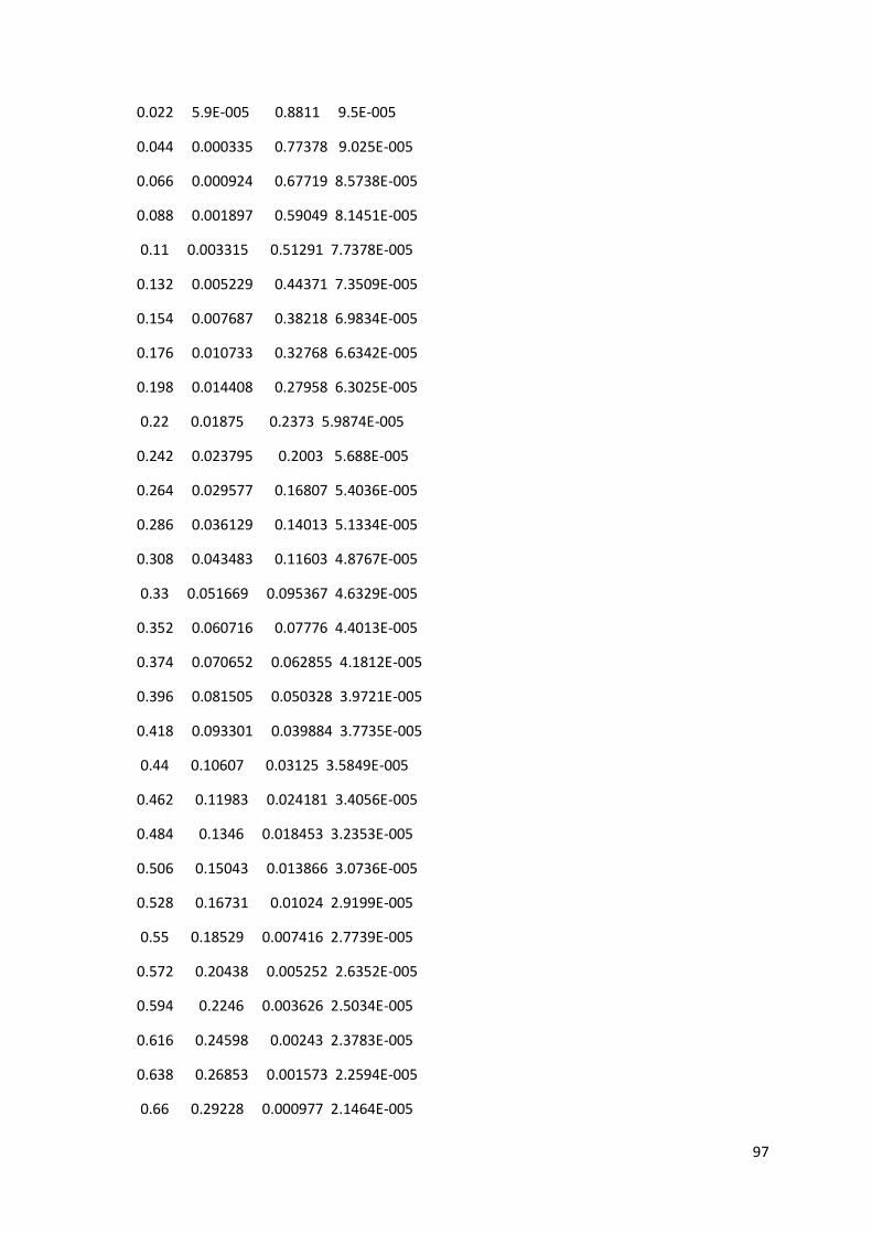
97
0.022 5.9E-005 0.8811 9.5E-005
0.044 0.000335 0.77378 9.025E-005
0.066 0.000924 0.67719 8.5738E-005
0.088 0.001897 0.59049 8.1451E-005
0.11 0.003315 0.51291 7.7378E-005
0.132 0.005229 0.44371 7.3509E-005
0.154 0.007687 0.38218 6.9834E-005
0.176 0.010733 0.32768 6.6342E-005
0.198 0.014408 0.27958 6.3025E-005
0.22 0.01875 0.2373 5.9874E-005
0.242 0.023795 0.2003 5.688E-005
0.264 0.029577 0.16807 5.4036E-005
0.286 0.036129 0.14013 5.1334E-005
0.308 0.043483 0.11603 4.8767E-005
0.33 0.051669 0.095367 4.6329E-005
0.352 0.060716 0.07776 4.4013E-005
0.374 0.070652 0.062855 4.1812E-005
0.396 0.081505 0.050328 3.9721E-005
0.418 0.093301 0.039884 3.7735E-005
0.44 0.10607 0.03125 3.5849E-005
0.462 0.11983 0.024181 3.4056E-005
0.484 0.1346 0.018453 3.2353E-005
0.506 0.15043 0.013866 3.0736E-005
0.528 0.16731 0.01024 2.9199E-005
0.55 0.18529 0.007416 2.7739E-005
0.572 0.20438 0.005252 2.6352E-005
0.594 0.2246 0.003626 2.5034E-005
0.616 0.24598 0.00243 2.3783E-005
0.638 0.26853 0.001573 2.2594E-005
0.66 0.29228 0.000977 2.1464E-005
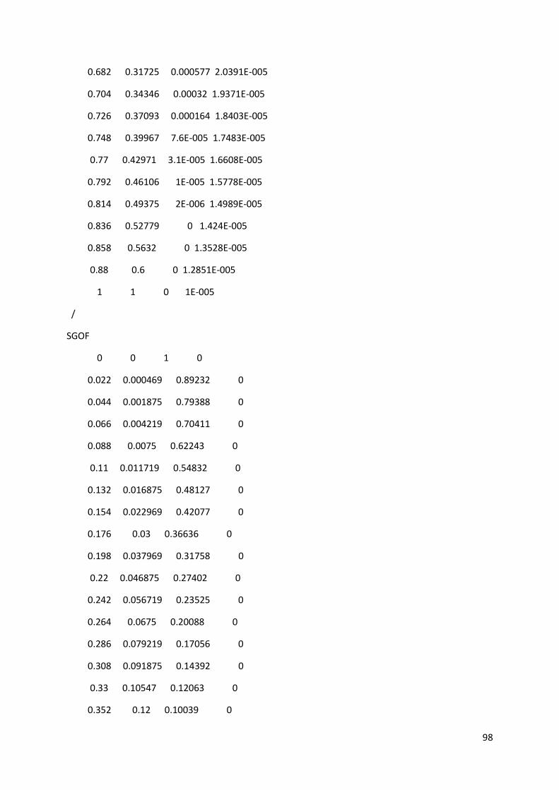
98
0.682 0.31725 0.000577 2.0391E-005
0.704 0.34346 0.00032 1.9371E-005
0.726 0.37093 0.000164 1.8403E-005
0.748 0.39967 7.6E-005 1.7483E-005
0.77 0.42971 3.1E-005 1.6608E-005
0.792 0.46106 1E-005 1.5778E-005
0.814 0.49375 2E-006 1.4989E-005
0.836 0.52779 0 1.424E-005
0.858 0.5632 0 1.3528E-005
0.88 0.6 0 1.2851E-005
1 1 0 1E-005
/
SGOF
0 0 1 0
0.022 0.000469 0.89232 0
0.044 0.001875 0.79388 0
0.066 0.004219 0.70411 0
0.088 0.0075 0.62243 0
0.11 0.011719 0.54832 0
0.132 0.016875 0.48127 0
0.154 0.022969 0.42077 0
0.176 0.03 0.36636 0
0.198 0.037969 0.31758 0
0.22 0.046875 0.27402 0
0.242 0.056719 0.23525 0
0.264 0.0675 0.20088 0
0.286 0.079219 0.17056 0
0.308 0.091875 0.14392 0
0.33 0.10547 0.12063 0
0.352 0.12 0.10039 0

99
0.374 0.13547 0.082891 0
0.396 0.15188 0.067863 0
0.418 0.16922 0.055045 0
0.44 0.1875 0.044194 0
0.462 0.20672 0.035085 0
0.484 0.22687 0.027508 0
0.506 0.24797 0.021269 0
0.528 0.27 0.016191 0
0.55 0.29297 0.01211 0
0.572 0.31688 0.008878 0
0.594 0.34172 0.00636 0
0.616 0.3675 0.004437 0
0.638 0.39422 0.002999 0
0.66 0.42188 0.001953 0
0.682 0.45047 0.001216 0
0.704 0.48 0.000716 0
0.726 0.51047 0.000392 0
0.748 0.54188 0.000196 0
0.77 0.57422 8.6E-005 0
0.792 0.6075 3.2E-005 0
0.814 0.64172 9E-006 0
0.836 0.67688 1E-006 0
0.858 0.71297 0 0
0.88 0.75 0 0
/
0 0 1 0
0.022 0.000469 0.89232 0
0.044 0.001875 0.79388 0
0.066 0.004219 0.70411 0
0.088 0.0075 0.62243 0
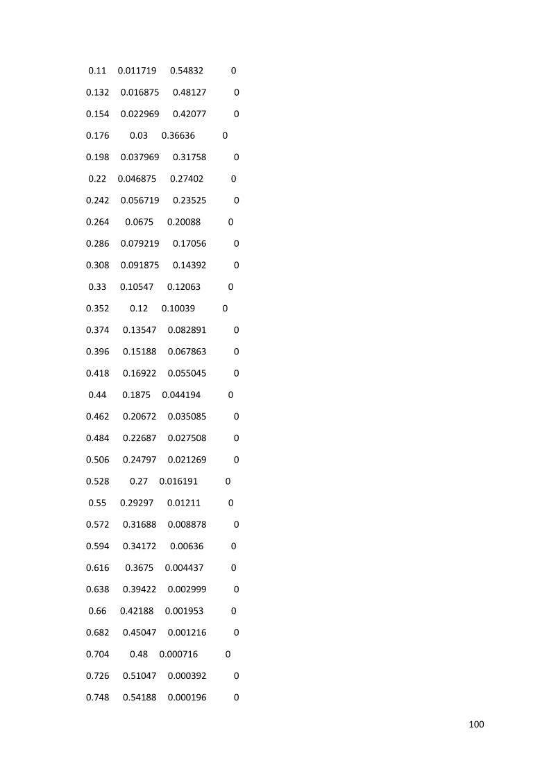
100
0.11 0.011719 0.54832 0
0.132 0.016875 0.48127 0
0.154 0.022969 0.42077 0
0.176 0.03 0.36636 0
0.198 0.037969 0.31758 0
0.22 0.046875 0.27402 0
0.242 0.056719 0.23525 0
0.264 0.0675 0.20088 0
0.286 0.079219 0.17056 0
0.308 0.091875 0.14392 0
0.33 0.10547 0.12063 0
0.352 0.12 0.10039 0
0.374 0.13547 0.082891 0
0.396 0.15188 0.067863 0
0.418 0.16922 0.055045 0
0.44 0.1875 0.044194 0
0.462 0.20672 0.035085 0
0.484 0.22687 0.027508 0
0.506 0.24797 0.021269 0
0.528 0.27 0.016191 0
0.55 0.29297 0.01211 0
0.572 0.31688 0.008878 0
0.594 0.34172 0.00636 0
0.616 0.3675 0.004437 0
0.638 0.39422 0.002999 0
0.66 0.42188 0.001953 0
0.682 0.45047 0.001216 0
0.704 0.48 0.000716 0
0.726 0.51047 0.000392 0
0.748 0.54188 0.000196 0

101
0.77 0.57422 8.6E-005 0
0.792 0.6075 3.2E-005 0
0.814 0.64172 9E-006 0
0.836 0.67688 1E-006 0
0.858 0.71297 0 0
0.88 0.75 0 0
/

102
'MB_REFERENCE_SCH.INC' /
RPTSCHED
FIP=3 WELLS=2 /
RPTRST
BASIC=3 FLOWS FREQ=10 /
WSEGITER
/
WELSPECS
PRMAIN PROD 51 42 1* OIL /
/
INCLUDE
'MB_REFERENCE_SCH_WELSEGS.INC' /
WSEGVALV
PRMAIN 2 1 0.012667 /
PRMAIN 3 1 0.012667 /
/
WLIST
'*PRODUCT' NEW
PRMAIN /
'*WELLS F' NEW
PRMAIN /
/
INCLUDE
'MB_REFERENCE_SCH_COMPDAT.INC' /
INCLUDE
'MB_REFERENCE_SCH_COMPSEGS.INC' /
INCLUDE
'MB_REFERENCE_SCH_PRMAIN.INC' /
GRUPTREE

103
INJ FIELD /
PROD FIELD /
/
WECON
PRMAIN 1* 1* 0.9500 1* 1* CON 1* 1* RATE 1* 1* 1* 100.00 /
/
WCONPROD
PRMAIN 1* GRUP 5* 70.0000 /
/
GRUPTREE
PROD FIELD /
/
GCONPROD
PROD NONE 2500.00 3500.00 900000.00 4000.00 RATE 1* 1* 1* RATE RATE
RATE /
/
GEFAC
PROD 0.9500 /
INJ 0.9500 /
/
TUNING
1 5* 0.01 /
/
2* 200 /
WSEGITER
-- MXWSIT mxnrtimes RedFac IncFac
70 70 0.25 3 /
DATES
1 JUN 2013 /
/

104
WELSPECS
INJREF INJ 55 23 1* WATER /
/
WLIST
'*INJECTI' NEW
INJREF /
'*WELLS F' ADD
INJREF /
/
WCONINJE
INJREF WATER 1* GRUP 5000.00 1* 225.0000 /
/
GPMAINT
FIELD WINS 0 1* 215.0000 10.0000 1.0000 /
/
WSEGFLIM
'PR*' 3 3 WAT 800 200 /
'PR*' 2 2 WAT 3500 200 /
/
ACTIONS
REDEAST2 'PR*' 3 SWCT > 0.7 2 /
/
WSEGFLIM
'PR*' 3 3 WAT 0 200 /
/
ENDACTIO
DATES
1 OCT 2013 /
/
DATES

105
1 JAN 2014 /
/
DATES
2 MAR 2014 /
/
DATES
1 NOV 2014 /
/
DATES
1 JAN 2015 /
/
DATES
2 MAR 2015 /
/
DATES
1 JAN 2016 /
/
DATES
2 MAR 2016 /
/
DATES
1 JAN 2017 /
/
DATES
2 MAR 2017 /
/
DATES
1 JAN 2018 /
/
DATES

106
2 MAR 2018 /
/
DATES
1 JAN 2019 /
/
DATES
2 MAR 2019 /
/
DATES
1 JAN 2020 /
/
DATES
2 MAR 2020 /
/
DATES
1 JAN 2021 /
/
DATES
2 MAR 2021 /
/
DATES
1 JAN 2022 /
/
DATES
2 MAR 2022 /
/
DATES
1 JAN 2023 /
/
DATES

107
2 MAR 2023 /
/
DATES
1 JAN 2024 /
/
DATES
2 MAR 2024 /
/
DATES
1 JAN 2025 /
/
DATES
2 MAR 2025 /
/
DATES
1 JAN 2026 /
/
DATES
2 MAR 2026 /
/
DATES
1 JAN 2027 /
/
DATES
2 MAR 2027 /
/
DATES
1 JAN 2028 /
/
DATES

108
2 MAR 2028 /
/
DATES
1 JAN 2029 /
/
DATES
2 MAR 2029 /
/
DATES
1 JAN 2030 /
/

![Master Thesis Outline: Draft 1 - [email protected] - University of](https://static.fdocuments.us/doc/165x107/620610888c2f7b1730045003/master-thesis-outline-draft-1-emailprotected-university-of.jpg)