
Master production schedule (MPS) - National Institute of ...nitc.ac.in/app/webroot/img/upload/Master...
30
National Institute of Technology Calicut Department of Mechanical Engineering MPS 1 March 2016 MASTER PRODUCTION SCHEDULE (MPS) Anticipated build schedule for manufacturing end products (or product options) A statement of production, not a statement of market demand MPS takes into account capacity limitations, as well as desires to utilize capacity fully Stated in product specifications – in part numbers for which bill of material exist Since it is a build schedule, it must be stated in terms used to determine component-part needs and other requirements; not in monetary or other global unit of measure Specific products may be groups of items such as models instead of end items The exact product mix may be determined with Final Assembly Schedule (FAS), which is not ascertained until the latest possible moment If the MPS is to be stated in terms of product groups, we must create a special bill of material (planning bill) for these groups Task performed by a master production scheduler Construct and update the MPS Involves processing MPS transactions, maintaining MPS records and reports, having a periodic review and update cycle (rolling through time), processing
Transcript of Master production schedule (MPS) - National Institute of ...nitc.ac.in/app/webroot/img/upload/Master...

National Institute of Technology Calicut Department of Mechanical Engineering
MPS 1 March 2016
MASTER PRODUCTION SCHEDULE (MPS)
Anticipated build schedule for manufacturing end
products (or product options)
A statement of production, not a statement of market
demand
MPS takes into account capacity limitations, as well as
desires to utilize capacity fully
Stated in product specifications – in part numbers for
which bill of material exist
Since it is a build schedule, it must be stated in terms
used to determine component-part needs and other
requirements; not in monetary or other global unit of
measure
Specific products may be groups of items such as models
instead of end items
The exact product mix may be determined with
Final Assembly Schedule (FAS), which is not
ascertained until the latest possible moment
If the MPS is to be stated in terms of product
groups, we must create a special bill of material
(planning bill) for these groups
Task performed by a master production scheduler
Construct and update the MPS
Involves processing MPS transactions, maintaining
MPS records and reports, having a periodic review
and update cycle (rolling through time), processing
National Institute of Technology Calicut Department of Mechanical Engineering
MPS 2 March 2016
and responding to exception conditions, and
measuring MPS effectiveness on a routine basis
On a day-to-day basis, marketing and production
are coordinated through the MPS in terms of Order
Promising
Order promising is the activity by which customer
order requests receive shipment dates
An effective MPS provides
Basis for making customer delivery promises
Utilising plant capacity effectively
Attaining the firm’s strategic objectives as reflected
in the production plan and
Resolving trade-off between manufacturing and
marketing
Since MPS is the basis for manufacturing budgets, the
financial budgets should be integrated with production
planning/MPS activities
When MPS is extended over a time horizon, is a better
basis for capital budgeting
Based on the production output specified in the MPS the
day-to-day cash flow can be forecasted
The MPS should be realizable and not overstated
When scheduled production exceeds capacity, usually
some or all of the following occur:
Invalid priority
Poor customer service (missed deliveries)

National Institute of Technology Calicut Department of Mechanical Engineering
MPS 3 March 2016
Excess in-process inventories
High expediting costs
Lack of accountability
Production
planning
Master
Production
Schedule
Resource
planning
Front End
Material
Requirements
Planning (MRP)
Material and
Capacity Plans
Detailed
Capacity
Planning
Engine
Purchasing
Systems
Shop-floor
Control
Systems Back End
Demand
management
Rough-cut
capacity
planning
Fig. 1: Manufacturing Planning and Control System
National Institute of Technology Calicut Department of Mechanical Engineering
MPS 4 March 2016
Linkage to Other Company Activities
The Demand Management Block
Represents a company’s forecasting, order entry, order
promising and physical distribution activities
Includes all activities that place demand on
manufacturing capacities
Demand may be actual and forecast customer orders,
branch warehouse requirements, interplant
requirements, international requirements and service
part requirements
The Production Plan Block
Represents role of production in the strategic business
plan of the company
Master
Scheduling
Capacity constraints
Forecasts
Production plan
Customer order
What to produce
When to produce
How much to produce
Product lead time constraints
Fig. 2: The Master Production Schedule
National Institute of Technology Calicut Department of Mechanical Engineering
MPS 5 March 2016
Reflects the desired aggregate output from
manufacturing necessary to support the company
game plan
The aggregate plan constraints the MPS, since the sum
of the detailed MPS quantities must always equal the
whole dictated by the production plan
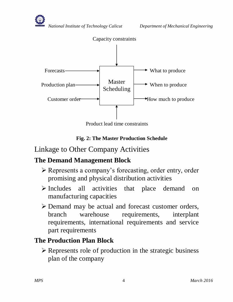
The Rough-cut Capacity Planning Block
Provides a rough evaluation of potential capacity
problems from a particular MPS
Structured Approach to Master Scheduling
Select the items and /or levels in the product structure
to be included in the master schedule
Determine the time horizon and time fences for the
master schedule
Obtain demand information for each item in the
schedule over the time horizon
Prepare tentative master schedule
Perform rough-cut capacity planning on the tentative
master schedule
Revise the tentative master schedule so it is capacity
feasible
Note on Master Schedule Stability
Freezing and time fencing concepts are used for stability
No changes (or changes only after tougher negotiations)
incorporated in certain number of recent periods of the
schedule in the case of freezing

National Institute of Technology Calicut Department of Mechanical Engineering
MPS 6 March 2016
Frozen period provides a stable target for manufacturing
to hit
Time fences specify periods in which various types of
changes can be handled
Two common fences are demand fence and planning
fence
Demand fence is the shorter of the two
Inside the demand fence, the forecast is ignored in
calculating the available
Within the demand fence it is very difficult to change the
MPS
Planning fence indicates the time at which the master
production scheduler should be planning more MPS
quantities
Between the demand fence and the planning fence,
management trade-offs must be made to make changes
Outside the planning fence, the master production
scheduler can make changes

National Institute of Technology Calicut Department of Mechanical Engineering
MPS 7 March 2016
DTF = Demand time fence; PTF = Planning time fence
Fig. 3: Master Schedule Time Fences
Business Environment and MPS
Encompasses the production approach used, the variety
of products produced, and the markets served by the
company
Based on the marketing environment the firms are
classified as
Make-to-stock, Make-to-order and Assemble-to-order
The MPS approach to this environment
The choice between these alternatives is largely one of
the unit (end items, specific customer orders, or some
group of end items and product options) used for the
MPS
Assemble Product Mfg. Parts Purchase Material Aggregate Plans
Cumulative lead time
Production Plan
Master schedule
Zone 1 Zone 2 Zone 3
Today DTF PTF

National Institute of Technology Calicut Department of Mechanical Engineering
MPS 8 March 2016
Make-to-stock
Produces in batches, carry finished goods inventories for
most end items
MPS is the production statement of how much of and
when each end items is to be produced
E.g.:- Consumer goods and supply items
Many organisations tend to group end items into model
grouping in the MPS preparation
The end item information is delayed until the latest
possible time and the end item schedule is available in
the final assembly schedule.
All product so grouped are run together in batches to
achieve economical run for component parts
Make-to-order
Carry no finished goods inventory and builds each
customer order as needed
Very large number of possible production configurations
Small probability of anticipating a customer’s exact need
Customers expect to wait for a large portion of the entire
design and manufacturing lead time
E.g.: - Special purpose machine tools
MPS unit is typically defined as the particular end item
or set of items comprising a customer order

National Institute of Technology Calicut Department of Mechanical Engineering
MPS 9 March 2016
Assemble-to-order
Limitless number of possible end item configurations, all
made from combination of basic components and
subassemblies
Customer delivery time is often shorter than total
manufacturing lead time
Large number of end item possibilities makes forecasting
exact end item configurations extremely difficult and
stocking end items very risky
Tries to maintain flexibility by starting basic components
and subassemblies into production and not starting final
assembly until a customer order is received
E.g.: - Dell computers
The MPS unit is stated in planning bills of material
The MPS unit (Planning bill) has its components as a set
of common parts and options
Note
Choice of MPS unit is somewhat open to definition by
the firm
Some firms may produce end items that are held in
inventory, yet still use assemble-to-order approaches
Some firms use more than one of these approaches at the
same time
Structural Features
Identifying the general product structure of an
organisation and locating the point of greatest

National Institute of Technology Calicut Department of Mechanical Engineering
MPS 10 March 2016
commonality – the narrowest part of the product
structure helps organisations to identify the MPS unit or
level
Fig. 4: General Product Structures
Table 1: Master Schedule Levels
Environment Forecast Master schedule level Classification
Make-to-stock End items End items Single-level
master schedule
Make-to-order
DLT PLT
None required End item from actual
orders
Single-level
master schedule
Make-to-order
DLT < PLT
Families with
planning bill
Family planning bill and percentage of end
items
Two-level
master schedule
Assemble-to-
order
Generic end item with
planning bill
Generic end item and
percentage of options
Two-level
master schedule
DLT = Delivery lead time; PLT = Product lead time
Finished
product
Limited number of
standard Items
assembled from
components
Finished
product
Many items made from
common subassemblies
Finished
product
Many items made from
limited number of
materials
National Institute of Technology Calicut Department of Mechanical Engineering
MPS 11 March 2016
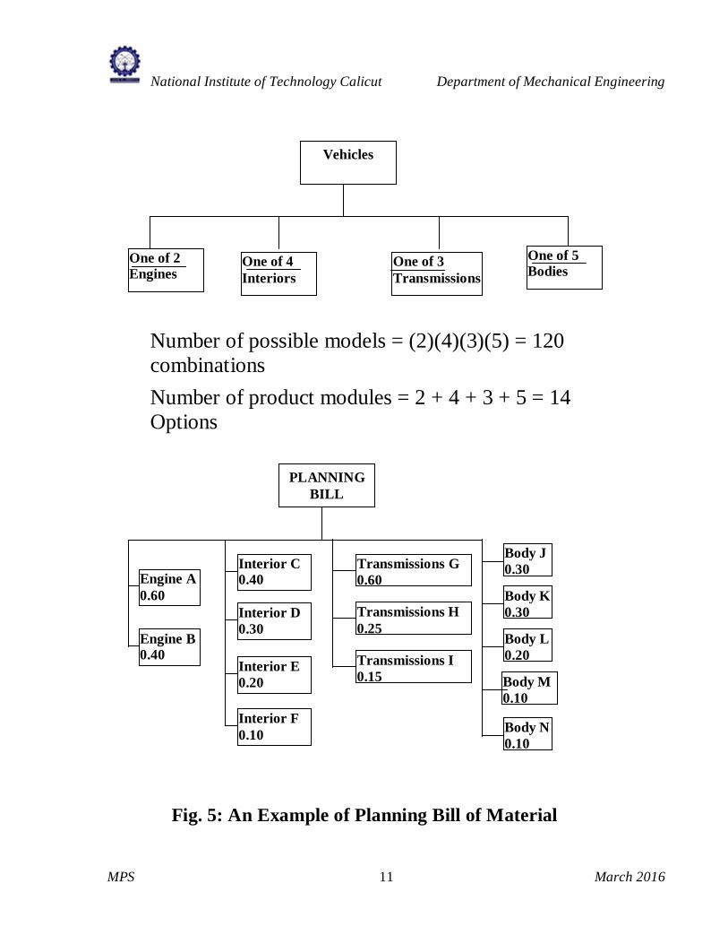
Number of possible models = (2)(4)(3)(5) = 120
combinations
Number of product modules = 2 + 4 + 3 + 5 = 14
Options
Fig. 5: An Example of Planning Bill of Material
One of 3
Transmissions
Vehicles
One of 2
Engines One of 4
Interiors
One of 5
Bodies
Engine A
0.60
Engine B
0.40
Transmissions H
0.25
Transmissions I
0.15
PLANNING
BILL
Interior C
0.40
Interior D
0.30
Interior E
0.20
Interior F
0.10
Transmissions G
0.60
Body J
0.30
Body K
0.30
Body L
0.20
Body M
0.10
Body N
0.10
National Institute of Technology Calicut Department of Mechanical Engineering
MPS 12 March 2016
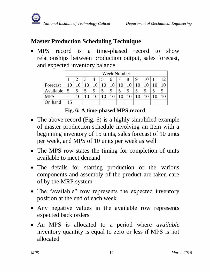
Master Production Scheduling Technique
MPS record is a time-phased record to show
relationships between production output, sales forecast,
and expected inventory balance
Week Number
1 2 3 4 5 6 7 8 9 10 11 12
Forecast 10 10 10 10 10 10 10 10 10 10 10 10
Available 5 5 5 5 5 5 5 5 5 5 5 5
MPS - 10 10 10 10 10 10 10 10 10 10 10
On hand 15
Fig. 6: A time-phased MPS record
The above record (Fig. 6) is a highly simplified example
of master production schedule involving an item with a
beginning inventory of 15 units, sales forecast of 10 units
per week, and MPS of 10 units per week as well
The MPS row states the timing for completion of units
available to meet demand
The details for starting production of the various
components and assembly of the product are taken care
of by the MRP system
The “available” row represents the expected inventory
position at the end of each week
Any negative values in the available row represents
expected back orders
An MPS is allocated to a period where available
inventory quantity is equal to zero or less if MPS is not
allocated

National Institute of Technology Calicut Department of Mechanical Engineering
MPS 13 March 2016
Reason for carrying positive projected inventory balance
Forecasts involve some degree of error, and the MPS
is a plan for production that may not be exactly
achieved
Projected inventory balance provides a tolerance for
errors that buffers production from sales variations
Various MPS approaches for seasonal products
The forecast for the next 12 weeks is given in Fig. 7 which
shows an average demand of 10 units and the MPS planner
plans 10 units as MPS in every week as the planner follows
a level strategy. Currently the planner has 20 units as on-
hand inventory. (This on-hand inventory, the planner
maintains to buffer against demand variability, and
production uncertainty which will be reflected as MPS
variability.) The MPS record in that case is as shown in
Fig. 7. Week Number
1 2 3 4 5 6 7 8 9 10 11 12
Forecast 5 5 5 5 5 5 15 15 15 15 15 15
Available 25 30 35 40 45 50 45 40 35 30 25 20
MPS 10 10 10 10 10 10 10 10 10 10 10 10
On hand 20
Fig. 7: Level Strategy
For the same situation given above (for the level strategy),
the MPS record, when chase strategy is followed, is given
in Fig. 8. In this strategy also the planner uses the on-hand
inventory to buffer against demand and MPS uncertainty.

National Institute of Technology Calicut Department of Mechanical Engineering
MPS 14 March 2016
Week Number
1 2 3 4 5 6 7 8 9 10 11 12
Forecast 5 5 5 5 5 5 15 15 15 15 15 15
Available 20 20 20 20 20 20 20 20 20 20 20 20
MPS 5 5 5 5 5 5 15 15 15 15 15 15
On hand 20
Fig. 8: Chase strategy
There are many alternative MPS plans possible between
these two extremes.
Lot sizing in MPS
Whenever an MPS is planned, the lot size is 30 units. The
record given in Fig. 9 shows that the MPS planner plans an
MPS quantity, when available quantity is zero or negative.
Week Number
1 2 3 4 5 6 7 8 9 10 11 12
Forecast 5 5 5 5 5 5 15 15 15 15 15 15
Available 15 10 5 30 25 20 5 20 5 20 5 20
MPS 30 30 30 30
On hand 20
Fig. 9: MPS with Lot sizing
Manufacturing in batches produces inventories that last
between production runs. This inventory is called cycle
stock.
Safety Stock in MPS
Revise the MPS in the Fig. 9 considering a safety stock
of 5 units. Assume that the on-hand contains the safety
stock. Fig. 10 shows the revised MPS record.
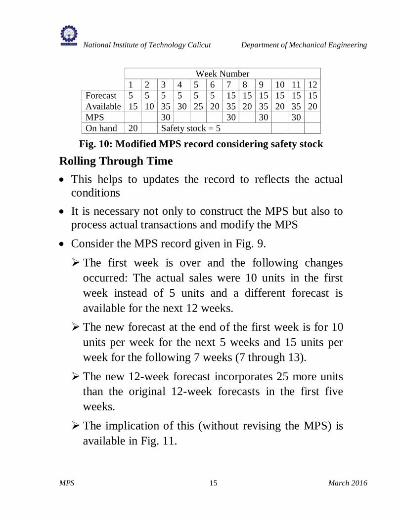
National Institute of Technology Calicut Department of Mechanical Engineering
MPS 15 March 2016
Week Number
1 2 3 4 5 6 7 8 9 10 11 12
Forecast 5 5 5 5 5 5 15 15 15 15 15 15
Available 15 10 35 30 25 20 35 20 35 20 35 20
MPS 30 30 30 30
On hand 20 Safety stock = 5
Fig. 10: Modified MPS record considering safety stock
Rolling Through Time
This helps to updates the record to reflects the actual
conditions
It is necessary not only to construct the MPS but also to
process actual transactions and modify the MPS
Consider the MPS record given in Fig. 9.
The first week is over and the following changes
occurred: The actual sales were 10 units in the first
week instead of 5 units and a different forecast is
available for the next 12 weeks.
The new forecast at the end of the first week is for 10
units per week for the next 5 weeks and 15 units per
week for the following 7 weeks (7 through 13).
The new 12-week forecast incorporates 25 more units
than the original 12-week forecasts in the first five
weeks.
The implication of this (without revising the MPS) is
available in Fig. 11.

National Institute of Technology Calicut Department of Mechanical Engineering
MPS 16 March 2016
Week Number
2 3 4 5 6 7 8 9 10 11 12 13
Forecast 10 10 10 10 10 15 15 15 15 15 15 15
Available 0 -10 10 0 -10 -25 -10 -25 -10 -25 -10 25
MPS 30 30 30 30
On hand 10
Fig. 11: Using the revised forecast after one week
The MPS record shown in Fig. 11 indicates that the plan
has several periods with shortages.
The planner revises the plan considering allocation of MPS
quantity in a period when available becomes zero or
negative is given in Fig. 12.
Week Number
2 3 4 5 6 7 8 9 10 11 12 13
Forecast 10 10 10 10 10 15 15 15 15 15 15 15
Available 30 20 10 30 20 5 20 5 20 5 20 5
MPS 30 30 30 30 30
On hand 10
Fig. 12: MPS revised to accommodate revised forecast after
one week
Identify the problems associated with the revised MPS
given in Fig. 12.
As per the plan in Fig. 9, the production department has to
give 30 units in week 4 of the production calendar, but the
revised plan asks this quantity by now (week 2 of
production calendar). This is impossible.

National Institute of Technology Calicut Department of Mechanical Engineering
MPS 17 March 2016
Production department has to give 30 units in week 5 as per
the plan in Fig. 12 which as per the plan in Fig. 9 is to
provide only in week 8. This is also a difficult task for the
production department.
Assume that the MPS planner was preparing the plan
with safety stock (of 15 units) regularly and as a result
the on-hand inventory for the first period is 35 units. The
plan in Fig. 9 modified on the basis of on-hand 35 units
and safety stock 15 is as shown in Fig. 13.
Week Number
1 2 3 4 5 6 7 8 9 10 11 12
Forecast 5 5 5 5 5 5 15 15 15 15 15 15
Available 30 25 20 45 40 35 20 35 20 35 20 35
MPS 30 30 30 30
On hand 35 Safety stock = 15
Fig. 13: MPS plan in Fig. 9 modified considering on-hand = 35
and safety stock = 15
When the plan is as shown in Fig. 13, the rolling through
time resulted in the plan as shown in Fig. 14. In this plan
no changes is made in MPS.
Week Number
2 3 4 5 6 7 8 9 10 11 12 13
Forecast 10 10 10 10 10 15 15 15 15 15 15 15
Available 15 5 25 15 5 -10 5 -10 5 -10 5 -10
MPS 30 30 30 30
On hand 25 Safety stock = 15
Fig. 14: Modified MPS plan in Fig.13 after rolling through
time
Fig. 14 shows that the severity of the problem due to
change in current demand and forecast are less compared to
the plan in Fig.11.

National Institute of Technology Calicut Department of Mechanical Engineering
MPS 18 March 2016
Order Promising
For many products, customers do not expect immediate
delivery, but place orders for future delivery
The delivery date (promise date) is negotiated through a
cycle of order promising, where the customer either asks
when the order can be shipped or specifies a desired
shipment date
If the company has a backlog of orders for future
shipments, the order promising task is to determine when
the shipment can be made
The delivery date promise procedure is explained with an
MPS record of an item shown below
Week Number
1 2 3 4 5 6 7 8 9 10 11 12
Forecast 5 5 5 5 5 5 15 15 15 15 15 15
Available 15 10 5 30 25 20 5 20 5 20 5 20
MPS 30 30 30 30
On hand 20
Fig. 15: A typical MPS plan for ATP incorporation
To decide the promise date the quantity available for
promise is to be known
Available-to-promise (ATP) is the term used to
represent this quantity
Conventions used in the MPS record with order promise
Forecast row shows the forecasting when items will be
shipped

National Institute of Technology Calicut Department of Mechanical Engineering
MPS 19 March 2016
There is a row labeled “Orders” represents the
company’s backlog of orders at the start of first week
The frequently used convention in the case of available
row is to use the greater of forecast or booked orders in
any period for projecting the available inventory balance
This is consistent with the concept that actual orders,
“consume” the forecast
That is, we start out with an estimate (the forecast), and
actual orders come into consume (either partially, fully,
or over the estimate)
Calculation procedure associated with available row is
Current period available = Previous period available +
MPS – (Greater of forecast or orders)
An ATP value is calculated for each period in which
there is an MPS quantity and also for the first period
To calculate the available to promise only the actual
orders and scheduled production are considered
ATP calculation procedure
Fist period ATP = On-hand + any first-period MPS -
(all orders until the next MPS)
Later period ATP = MPS in that period - (all orders
in that and subsequent periods until the next MPS)
Both of these rules, however, have to be modified to
reflect subsequent periods ATP deficiencies

National Institute of Technology Calicut Department of Mechanical Engineering
MPS 20 March 2016
Week Number
1 2 3 4 5 6 7 8 9 10 11 12
Forecast 5 5 5 5 5 5 15 15 15 15 15 15
Orders 5 3 2
Available 15 10 5 30 25 20 5 20 5 20 5 20
ATP 10 30 30 30 30
MPS 30 30 30 30
On hand 20
Fig. 16: MPS record with ATP
Suppose an order for 35 units was booked for week 10 in
the current period for the above item
The ATP row changes as follows
Week Number
1 2 3 4 5 6 7 8 9 10 11 12
Forecast 5 5 5 5 5 5 15 15 15 15 15 15
Orders 5 3 2 35
Available 15 10 5 30 25 20 5 20 5 0 -15 0
ATP 10 30 25 0 30
MPS 30 30 30 30
On hand 20
Fig. 17: MPS Record with ATP showing ATP calculation
under subsequent period ATP deficiency
Note that the later customer orders are covered by the
later MPS quantities
The 35 units order for week 10 could have been covered
by 10 units in week 1 plus 25 units from the MPS of
week 4.

National Institute of Technology Calicut Department of Mechanical Engineering
MPS 21 March 2016
This would have left no units for promising from week 1
until week 3, greatly reducing promise flexibility
The convention is to preserve early promise flexibility by
allocating units to actual orders as late as possible
The available row provides the master production
scheduler with a projection of the item availability
throughout the planning horizon
This is important information for managing the master
production schedule
A negative available quantity at the end of the planning
horizon is a signal for more MPS
During the planning horizon there is typically some
length of time in which changes are to be made only if
absolutely essential, to provide stability for planning and
execution
At the end of this period, master production schedulers
have maximum flexibility to create additional MPS
quantity
Accurate order promising allows the company to operate
with reduced inventory levels
That is, order promising allows the actual shipments to
be closer to the MPS
Companies in effect buffer uncertainties in demand by
their delivery date promises
Firms manage the delivery dates rather than carry safety
stock to absorb uneven customer order pattern

National Institute of Technology Calicut Department of Mechanical Engineering
MPS 22 March 2016
Exercise Problem
1. Problem
Neptune Manufacturing Company’s production manager
wants a master production schedule covering next year’s
business. The company produces a complete line of small
fishing boats for both saltwater and freshwater use and
manufactures most of the components part used in
assembling the products. The firm uses MRP to coordinate
production schedule of the component part manufacturing
and assembly operations. The production manager has just
received the following sales forecast for next year from the
marketing division:
Product
Lines
Sales Forecast (standard boats for each series)
1st Quarter 2
nd Quarter 3
rd Quarter 4
th Quarter
FunRay
series
8,000 9,000 6,000 6,000
SunRay
series
4,000 5,000 2,000 2,000
StingRay
Series
9,000 10,000 6,000 7,000
Total 21,000 24,000 14,000 15,000
The sales forecast is stated in terms of “standard boats”,
reflecting total sales volume for each of the firm’s three
major product lines.
Another item of information supplied by marketing
department is the target ending inventory position for each
product line. The marketing department would like the
production manager to plan on having the following
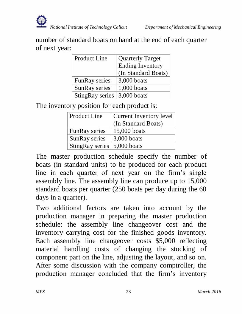
National Institute of Technology Calicut Department of Mechanical Engineering
MPS 23 March 2016
number of standard boats on hand at the end of each quarter
of next year:
Product Line Quarterly Target
Ending Inventory
(In Standard Boats)
FunRay series 3,000 boats
SunRay series 1,000 boats
StingRay series 3,000 boats
The inventory position for each product is:
Product Line Current Inventory level
(In Standard Boats)
FunRay series 15,000 boats
SunRay series 3,000 boats
StingRay series 5,000 boats
The master production schedule specify the number of
boats (in standard units) to be produced for each product
line in each quarter of next year on the firm’s single
assembly line. The assembly line can produce up to 15,000
standard boats per quarter (250 boats per day during the 60
days in a quarter).
Two additional factors are taken into account by the
production manager in preparing the master production
schedule: the assembly line changeover cost and the
inventory carrying cost for the finished goods inventory.
Each assembly line changeover costs $5,000 reflecting
material handling costs of changing the stocking of
component part on the line, adjusting the layout, and so on.
After some discussion with the company comptroller, the
production manager concluded that the firm’s inventory

National Institute of Technology Calicut Department of Mechanical Engineering
MPS 24 March 2016
carrying cost is 10 percent of standard boats cost per year.
The item value for each of the product line standard units
is:
Product Line Standard Boat Cost
FunRay series $ 100
SunRay series 150
StingRay series 200
The master production scheduler has calculated the
production lot sizes as 5,000, 3,000 and 4,000 units,
respectively.
a) Develop a master production schedule for next year, by
quarter, for Neptune’s fishing boat line. Identify any
problems.
b) Verify the lot size calculations using the EOQ formula.
Solution for part (a) of the problem
When the MPS is prepared here, the constraints to be
satisfied are demand, capacity, end of the period inventory
and lot sizing. Prepare a tentative MPS satisfying demand
and lot sizing constraints. If the planned production is more
than the lot size, the production batch is determined as the
planned quantity for meeting the requirements.
FunRay Series
Period 1 2 3 4
Forecast 8000 9000 6000 6000
Available 7000 3000 2000 1000
MPS 5000 5000 5000
On-hand 15,000

National Institute of Technology Calicut Department of Mechanical Engineering
MPS 25 March 2016
SunRay Series Period 1 2 3 4
Forecast 4000 5000 2000 2000
Available 2000 -- 1000 2000
MPS 3000 3000 3000 3000
On-hand 3,000
StingRay Series Period 1 2 3 4
Forecast 9000 10,000 6000 7000
Available -- -- -- --
MPS 4000 10,000 6000 7000
On-hand 5000
Scheduled production for assembly line FunRay series -- 5000 5000 5000
SunRay series 3000 3000 3000 3000
StingRay series 4000 10,000 6000 7000
Total 7000 18,000 14,000 15,000
MPS quantity in 2nd quarter is higher than the capacity.
Also, the required quarterly ending inventory is not
achieved using the tentative MPS.
Now, considering the excess capacity available in certain
period, try to satisfy the capacity constraint. The capacity
and demand constraints should be satisfied, and the lot
sizing and end of the period inventory constraints should be
satisfied to the maximum possible extend.
National Institute of Technology Calicut Department of Mechanical Engineering
MPS 26 March 2016
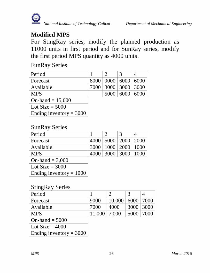
Modified MPS
For StingRay series, modify the planned production as
11000 units in first period and for SunRay series, modify
the first period MPS quantity as 4000 units.
FunRay Series
Period 1 2 3 4
Forecast 8000 9000 6000 6000
Available 7000 3000 3000 3000
MPS 5000 6000 6000
On-hand = 15,000
Lot Size = 5000
Ending inventory = 3000
SunRay Series Period 1 2 3 4
Forecast 4000 5000 2000 2000
Available 3000 1000 2000 1000
MPS 4000 3000 3000 1000
On-hand = 3,000
Lot Size = 3000
Ending inventory = 1000
StingRay Series Period 1 2 3 4
Forecast 9000 10,000 6000 7000
Available 7000 4000 3000 3000
MPS 11,000 7,000 5000 7000
On-hand = 5000
Lot Size = 4000
Ending inventory = 3000
National Institute of Technology Calicut Department of Mechanical Engineering
MPS 27 March 2016
MPS quantities for assembly line FunRay series 5000 6000 6000
SunRay series 4000 3000 3000 1000
StingRay series 11,000 7,000 5000 7000
Total 15,000 15,000 14,000 14,000
Above MPSs are satisfying production capacity constraints
and end of the period inventory constraints. The lot sizing
constraints are satisfied under the modified rule (If MPS
quantity is greater than suggested lot size, then the lot size
is equal to MPS quantity.). But this constraint is not
satisfied for period 4 of SunRay series. The constraints -
the end of the period inventory given is considered as the
minimum requirement.
Think of some modification for SunRay series considering
excess capacity available in period 3 and without any MPS
quantity in period 4.
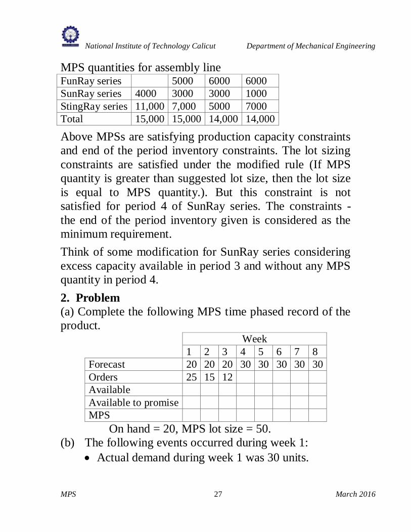
2. Problem
(a) Complete the following MPS time phased record of the
product. Week
1 2 3 4 5 6 7 8
Forecast 20 20 20 30 30 30 30 30
Orders 25 15 12
Available
Available to promise
MPS
On hand = 20, MPS lot size = 50.
(b) The following events occurred during week 1:
Actual demand during week 1 was 30 units.

National Institute of Technology Calicut Department of Mechanical Engineering
MPS 28 March 2016
Marketing forecasted that 40 units would be needed
for week 9.
An order for 10 in week 2 was accepted.
An order for 20 in week 4 was accepted.
An order for 60 in week 6 was accepted.
The MPS in week 1 was produced as planned.
Update the record after rolling through time. Assume that
the demand time fence (DTF) is 4 weeks. Management is
not interested to make any change in quantity and period of
MPSs in DTF. Do you have any difficulty after rolling
through week 1?
Solution
(a) Week
1 2 3 4 5 6 7 8
Forecast 20 20 20 30 30 30 30 30
Orders 25 15 12
Available 45 25 5 25 45 15 35 5
Available to promise 18 50 50 50
MPS 50 50 50 50
On hand = 20, MPS lot size = 50.
(b) When the record is processed at the end of week 1 and
no change in MPS is made in DTF, the MPS record is as
follows:

National Institute of Technology Calicut Department of Mechanical Engineering
MPS 29 March 2016
Week
2 3 4 5 6 7 8 9
Forecast 20 20 30 30 30 30 30 40
Orders 25 12 20 60
Available 15*
3*
33*
83*
23 43 13 23
Available to promise 3 20 0**
50 50
MPS 50 50 50 50
On hand = 40, MPS lot size = 50.
* Only orders are considered for available to calculate
** If you use the ATP (available to promise) calculation
method, the ATP quantity is negative. But the ATP
quantity available in the immediate previous period is used
to meet the actual order of succeeding period and hence the
ATP for the period 5 is made zero. Note that the later
customer orders are covered by the later MPS quantities.
Incorporation of MPS execution related information in
the MPS record
Consider the record in the part (a) of problem 2. Assume
that the lead time for this item is two weeks when its
immediate components (i.e., first level item in its bill of
material) are available. The record can be modified to
include the planned order release and scheduled receipt.
The MPS = 50 units in week 1 of the record shows that 50
units will be received in the beginning of week 1 to the
finished goods inventory. That is, a production order might
have been released in an early week and based on this
production order, production activities might be going-on

National Institute of Technology Calicut Department of Mechanical Engineering
MPS 30 March 2016
in the production shops. The record will be more
informative if the order receipt and order releases are
shown in it. The record below shows these details in an
MPS record.
Week
1 2 3 4 5 6 7 8
Forecast 20 20 20 30 30 30 30 30
Orders 25 15 12
Available 45 25 5 25 45 15 35 5
Available to promise 18 50 50 50
MPS 50 50 50 50
Scheduled receipt 50
Planned order release 50 50 50