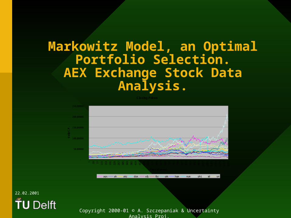
Markowitz Model, an Optimal Portfolio Selection.

AEX Exchange Stock Data Analysis.

Copyright 2000-01 © A. Szczepaniak & Uncertainty Analysis Proj.

Closing Prices

-

50,00000

100,00000

150,00000

200,00000

250,00000

1 39 77 115

153

191

229

267

305

343

381

419

457

495

533

571

609

647

685

723

761

799

837

875

913

951

989

1027

1065

1103

1141

1179

1217

1255

Time (5 years)

Dai

ly C

.P.

agn ah akz dsm els for gtn hgm num phi rd un

22.02.2001

2

Harry Markowitz

Got Nobel Prize in Economy together with William Sharpe and Merton Miller because of their modern portfolio selection models theorem. Basically the main idea was to eliminate very complicated company analysis and BASED PORTFOLIO SELECTION ONLY ON the MATHEMATICAL CALCULATION.

Necessary definitions:

Portfolio --- a collection of investments. Expected risk --- the total amount of money that can be Lost. Expected return --- future income from invested capital. “Portfolio effect” --- portfolio that will reduce total risk of Investment. Portfolio manager --- projekt manager Efficient portfolio --- provides the lowest expected risk for a given expected return, or the greatest expected return for a given level of risk.

3

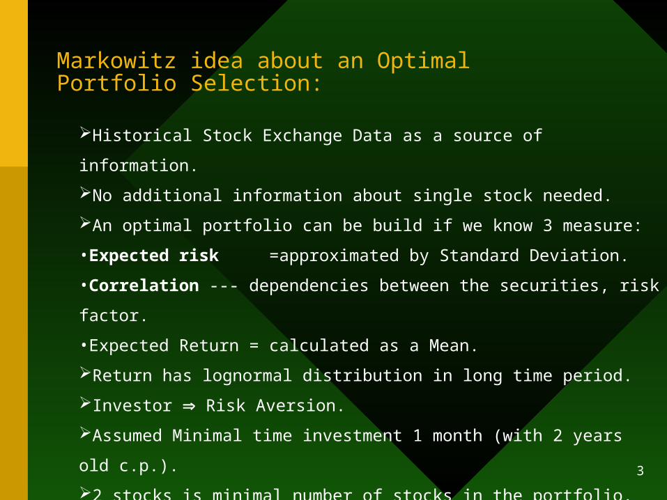
Markowitz idea about an Optimal Portfolio Selection:

Historical Stock Exchange Data as a source of information.

No additional information about single stock needed.

An optimal portfolio can be build if we know 3 measure:

•Expected risk =approximated by Standard Deviation.

•Correlation --- dependencies between the securities, risk factor.

•Expected Return = calculated as a Mean.

Return has lognormal distribution in long time period.

Investor Risk Aversion.

Assumed Minimal time investment 1 month (with 2 years old c.p.).

2 stocks is minimal number of stocks in the portfolio.

4

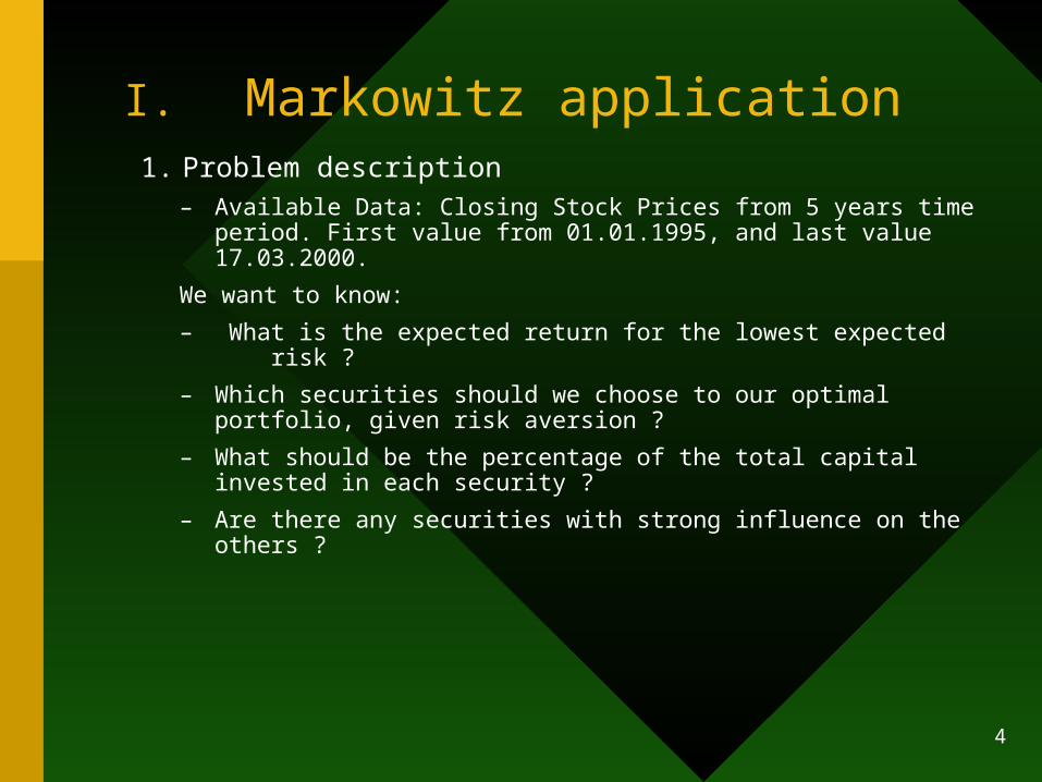
I. Markowitz application1. Problem description

– Available Data: Closing Stock Prices from 5 years time period. First value from 01.01.1995, and last value 17.03.2000.

We want to know:

– What is the expected return for the lowest expected risk ?

– Which securities should we choose to our optimal portfolio, given risk aversion ?

– What should be the percentage of the total capital invested in each security ?

– Are there any securities with strong influence on the others ?

5

II. Model description2.1 Basic idea (Unconditional case):

• P =Alfa*A+(1-Aalfa)*B

A,B --- known stock closing prices. Alfa --- percentage of all amount of money invested in given stock. P --- basic portfolio, consists of 2 stocks.

• More general formula, portfolio made for n-stocks:

Ci – percentage of all amount of money invested in given stock.

Ai – some stock denoted as i-th of all n.

i

n

iiACP

11

1

n

iiC

6

Using Markowitz Model:

Expected return for the portfolio P is E(P)=Alfa*E(A)+(1-Alfa)*E(B)

Expected risk for portfolio P is SQRT(Var(P)) is

P=

where p(A,B) is correlation between stocks A&B.

• Now we have the following optimisation problem:

Minimize SQRT(Var(P)) where Alfa[0,1], get E(P).

We can assume in addition that our E(P)c where c > 0 and c=const.

BABA BA )1(),(2)1( 2222

7

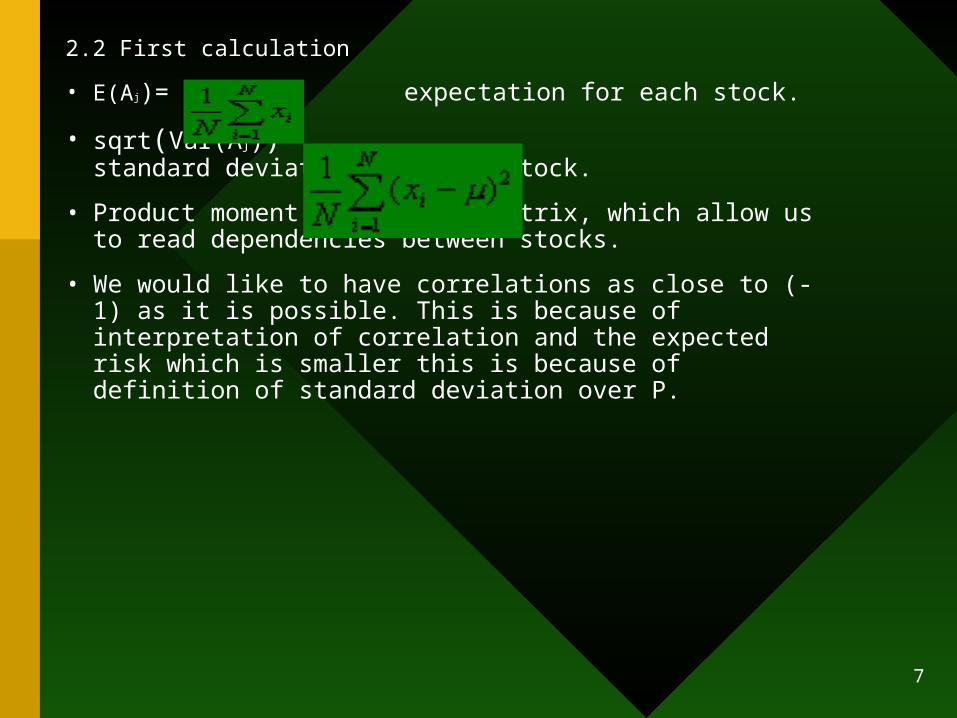
2.2 First calculation

• E(Aj)= expectation for each stock.

• sqrt(Var(Aj))= standard deviation for each stock.

• Product moment correlation matrix, which allow us to read dependencies between stocks.

• We would like to have correlations as close to (-1) as it is possible. This is because of interpretation of correlation and the expected risk which is smaller this is because of definition of standard deviation over P.

8

2.3 Results.Product moment correlation matrix. Picture interpretation:

if all lines between two stocks are horizontal then product moment correlation let as say =1 if all lines between two stocks cross in one point then =-1 if all lines between two stocks criss-cross in such way that the density between crossing is triangular then =0.

9

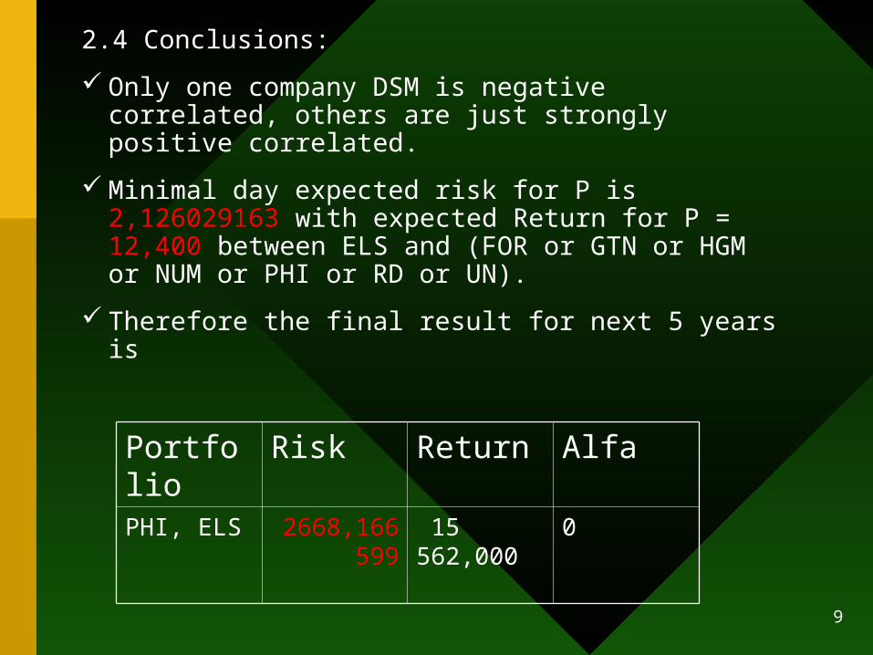
2.4 Conclusions:

Only one company DSM is negative correlated, others are just strongly positive correlated.

Minimal day expected risk for P is 2,126029163 with expected Return for P = 12,400 between ELS and (FOR or GTN or HGM or NUM or PHI or RD or UN).

Therefore the final result for next 5 years is

Portfolio Risk Return AlfaPHI, ELS 2668,1665

99 15 562,000

0

10

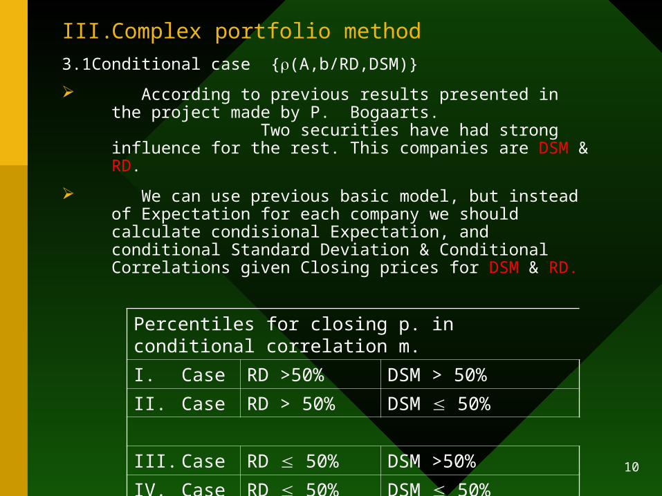
III. Complex portfolio method

3.1Conditional case {(A,b/RD,DSM)}

According to previous results presented in the project made by P. Bogaarts. Two securities have had strong influence for the rest. This companies are DSM & RD.

We can use previous basic model, but instead of Expectation for each company we should calculate condisional Expectation, and conditional Standard Deviation & Conditional Correlations given Closing prices for DSM & RD.

Percentiles for closing p. in conditional correlation m.

I. Case RD >50% DSM > 50%

II. Case RD > 50% DSM 50%

III. Case RD 50% DSM >50%

IV. Case RD 50% DSM 50%

11

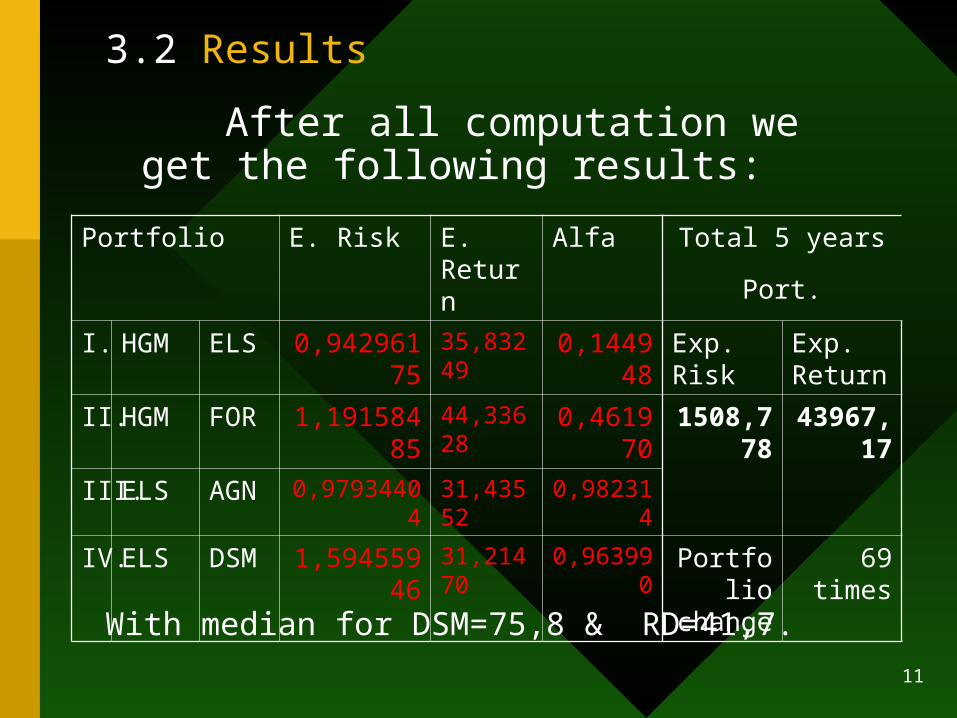
3.2 Results

After all computation we get the following results:

Portfolio E. Risk E. Return

Alfa Total 5 years

Port.

I. HGM ELS 0,94296175

35,83249

0,144948

Exp. Risk

Exp. Return

II. HGM FOR 1,19158485

44,33628

0,461970

1508,778

43967,17

III. ELS AGN 0,97934404 31,43552

0,982314

IV. ELS DSM 1,59455946

31,21470

0,963990 Portfolio change

69 times

With median for DSM=75,8 & RD=41,7.

12

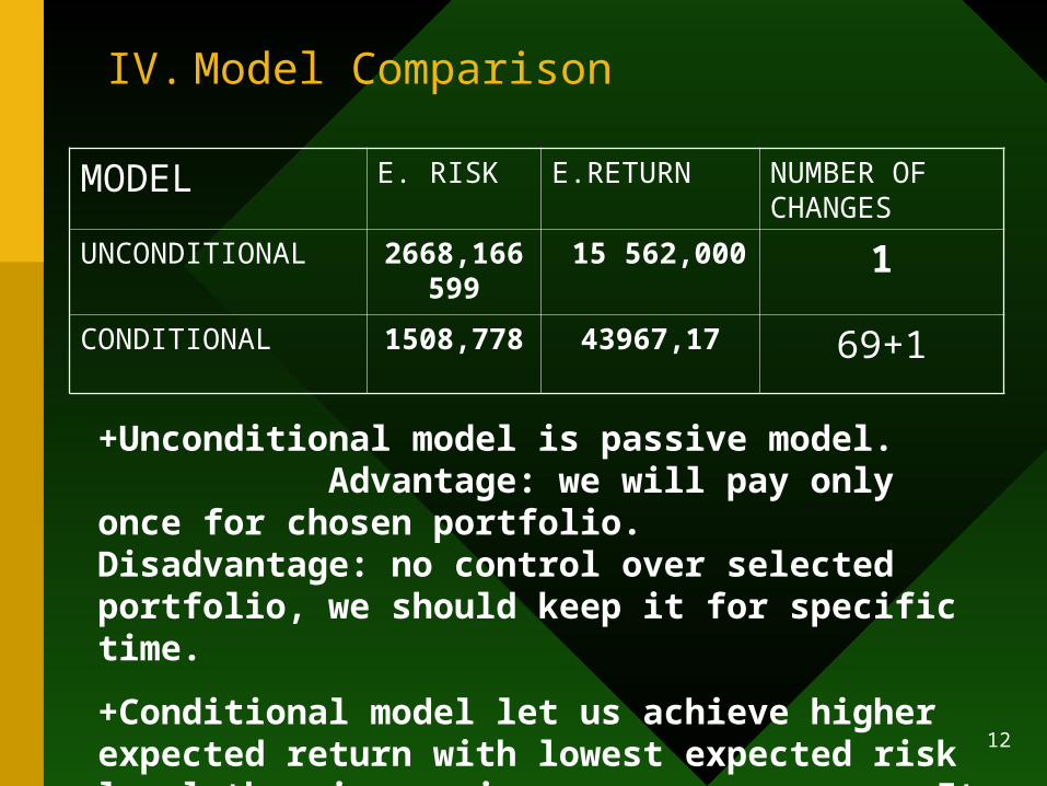
IV. Model Comparison

MODEL E. RISK E.RETURN NUMBER OF CHANGES

UNCONDITIONAL 2668,166599

15 562,000 1

CONDITIONAL 1508,778 43967,17 69+1

+Unconditional model is passive model. Advantage: we will pay only once for chosen portfolio. Disadvantage: no control over selected portfolio, we should keep it for specific time.

+Conditional model let us achieve higher expected return with lowest expected risk level then in previous case. It is active model which can be upgraded every day. Advantage: strict control over portfolio.

13

V. First simulation5.1 Method Description

We were adding to historical data 260 day closing prices of RD & DSM.

Created macros were checking given conditions and returned composition of portfolio in CONDITIONAL case and percentage of money invested in each security for single day.

Macro for UNCONDITIONAL case simple follows past results and apply expected risk and return daily.

14

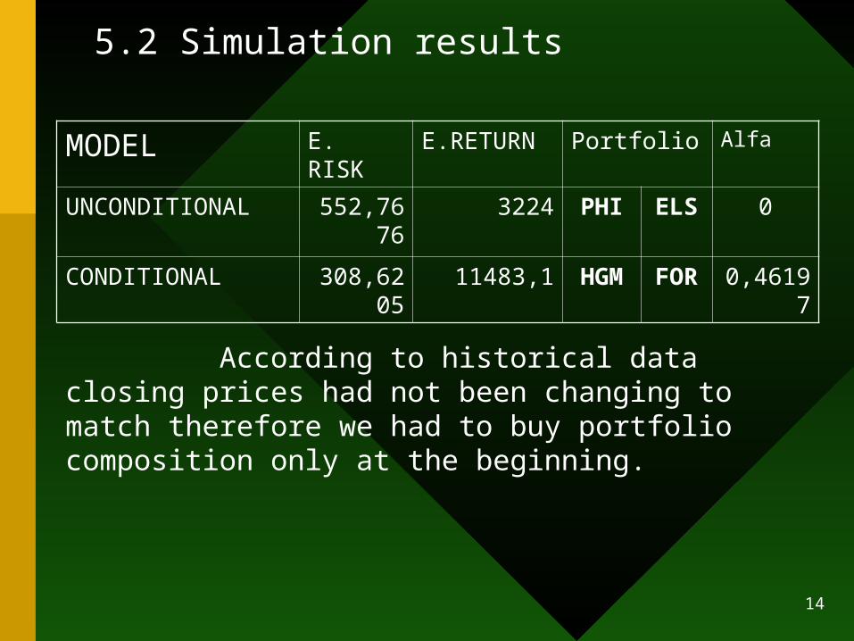
5.2 Simulation results

MODEL E. RISK E.RETURN Portfolio Alfa

UNCONDITIONAL 552,7676

3224 PHI ELS 0

CONDITIONAL 308,6205

11483,1 HGM FOR 0,46197

According to historical data closing prices had not been changing to match therefore we had to buy portfolio composition only at the beginning.

15

VI. Possible improvements.

• Apply described method for n stocks. Restriction: optimal number of stocks between 8 and 20. Bigger number of securities is expensive during changes and time computation.

• Upgrade owned data untill current day and buy securities on the AEX – index stock exchange.