Markov models for linking environments and facies in...
42
Riegl and Purkis “Markov and graph theory on carbonate landscapes’ 1 Markov models for linking environments and facies in space and time (Recent Arabian Gulf, Miocene Paratethys) BERNHARD M. RIEGL and SAMUEL J. PURKIS National Coral Reef Institute, Nova Southeastern University Oceanographic Center, 8000 N. Ocean Drive, Dania FL 33004 ABSTRACT If, as comparative sedimentology maintains, knowledge of the Recent can sometimes be helpful to explain the past (and vice-versa), common quantitative denominators might exist between Recent and fossil systems. It may also be possible to describe dynamics and find linkages between space and time with a unique set of quantitative tools. To explore such conceptual links, spatial facies patterns mapped using satellite imagery were compared with temporal patterns in analogous ancient outcropping facies using Markov chains and graphs. Landsat and Ikonos satellite imagery was used to map benthic facies in a nearshore carbonate ramp (Ras Hasyan) and offshore platform system (Murrawah, Al Gharbi) in the Recent Arabian Gulf (United Arab Emirates), and results were compared to the Fenk quarry outcrop in Burgenland, Austria, a carbonate ramp of the Miocene (Badenian) Paratethys. Facies adjacencies (i.e. Moore neighbourhood of colour-coded image pixels of satellite image or outcrop map) were expressed by transition probability matrices which showed that horizontal (spatial) facies sequences and vertical (temporal) outcrop sequences had the Markov property (knowledge of t-th state defines likelihoods of t+1 st state) and that equivalent facies were comparable in frequency. We expressed the transition probability matrices as weighted digraphs and calculated fixed probability vectors which encapsulate information on both the spatial and temporal components (size of and time spent in each facies). Models of temporal functioning were obtained by modifying matrices (digraphs) of spatial adjacency to matrices (digraphs) of temporal adjacency by using the same vertices (facies) but adjusting transitions without changing paths. With this combined spatio-temporal model, we investigated changes in facies composition in falling and rising sea-level scenarios by adjusting transition likelihoods preferentially into shallower (falling sea-level) or deeper (rising sea-level) facies. Our model can also be used as a numerical analogue to a Ginsburg-type autocyclic model. The fixed probability vector was used as a proxy for final facies distribution. Using Markov chains it is possible to use vertical outcrop data to evaluate the relative contribution of each facies in any time-slice which can aid, for example, in estimation of
Transcript of Markov models for linking environments and facies in...

Riegl and Purkis “Markov and graph theory on carbonate landscapes’ 1
Markov models for linking environments and facies in space
and time (Recent Arabian Gulf, Miocene Paratethys)
BERNHARD M. RIEGL and SAMUEL J. PURKIS
National Coral Reef Institute, Nova Southeastern University Oceanographic Center, 8000 N. Ocean Drive,
Dania FL 33004
ABSTRACT
If, as comparative sedimentology maintains, knowledge of the Recent can sometimes be
helpful to explain the past (and vice-versa), common quantitative denominators might
exist between Recent and fossil systems. It may also be possible to describe dynamics
and find linkages between space and time with a unique set of quantitative tools. To
explore such conceptual links, spatial facies patterns mapped using satellite imagery were
compared with temporal patterns in analogous ancient outcropping facies using Markov
chains and graphs. Landsat and Ikonos satellite imagery was used to map benthic facies
in a nearshore carbonate ramp (Ras Hasyan) and offshore platform system (Murrawah, Al
Gharbi) in the Recent Arabian Gulf (United Arab Emirates), and results were compared
to the Fenk quarry outcrop in Burgenland, Austria, a carbonate ramp of the Miocene
(Badenian) Paratethys. Facies adjacencies (i.e. Moore neighbourhood of colour-coded
image pixels of satellite image or outcrop map) were expressed by transition probability
matrices which showed that horizontal (spatial) facies sequences and vertical (temporal)
outcrop sequences had the Markov property (knowledge of t-th state defines likelihoods
of t+1st state) and that equivalent facies were comparable in frequency. We expressed the
transition probability matrices as weighted digraphs and calculated fixed probability
vectors which encapsulate information on both the spatial and temporal components (size
of and time spent in each facies). Models of temporal functioning were obtained by
modifying matrices (digraphs) of spatial adjacency to matrices (digraphs) of temporal
adjacency by using the same vertices (facies) but adjusting transitions without changing
paths. With this combined spatio-temporal model, we investigated changes in facies
composition in falling and rising sea-level scenarios by adjusting transition likelihoods
preferentially into shallower (falling sea-level) or deeper (rising sea-level) facies. Our
model can also be used as a numerical analogue to a Ginsburg-type autocyclic model.
The fixed probability vector was used as a proxy for final facies distribution. Using
Markov chains it is possible to use vertical outcrop data to evaluate the relative
contribution of each facies in any time-slice which can aid, for example, in estimation of

Riegl and Purkis “Markov and graph theory on carbonate landscapes’ 2
reservoir sizes and to gain insight into temporal functioning as derived from spatial
pattern.
Keywords: Arabian Gulf, Leitha Limestone, Paratethys, Markov chain, comparative
sedimentology, Walther’s Law, landscape pattern, remote sensing, carbonate
sedimentation
INTRODUCTION
The actualistic principle and comparative sedimentology see the present as a key to the past (Ginsburg
1974). Additionally, a liberal interpretation of Walther’s Law (Middleton, 1973) might suggest that in some
special cases the past may even hold a key to the present or future, since knowledge of the conformable
strata in outcrop, if time-transgressive, might allow some reconstruction of the lateral facies mosaic in any
time-slice, be it in the past or the present (Doveton, 1994; Parks et al., 2000). All this suggests that a
quantitative expression of temporal information from core or outcrop into spatial information on a map of a
landscape, and vice versa, would be interesting and in the tradition of comparative sedimentology
(Ginsburg, 1974; 1975).
Invoking the present for reconstruction of the past obviously requires some understanding of its
functioning. Geology and biology merge in shallow, tropical carbonate systems since ecology and
successional stages of organismal communities influence the development of facies and vice versa
(Ginsburg, 1957; Toomey, 1981; Schlager, 2005). While the environment (climate, tectonism, eustasy, etc.)
controls lateral dimensions and vertical successional pattern (James, 1984; Wilgus et al., 1989; Tucker &
Wright, 1990; Wilkinson et al., 1997; Lehrmann & Goldhammer, 1999; Wilkinson et al., 2003; Rankey,
2004; Schlager, 2005), ecology often defines facies at a finer scale (Flügel, 2004).
In numerous previous studies, Markov chains have shown that conditional probabilistic relationships
(knowledge of an event/facies will define probability of a following event/facies) exist among vertical
facies successions (Krumbein, 1967; Krumbein & Greybull, 1967; Gingerich, 1969; Doveton, 1971, 1994;
Miall, 1973; Carle & Fogg, 1997; Wilkinson et al., 1997; Lehrmann & Rankey, 1999; Parks et al., 2000;
Davis, 2002; Wilkinson et al., 2003). Stages of ecological community and landscape successions have
Markovian properties (Pielou 1969; Horn, 1975, Usher, 1979; Urban & Wallin 2002; Turner et al., 2001)
which can be expressed using graphs (Roberts 1976; Cantwell & Forman, 1993; Bunn et al., 2000; Urban
& Keitt, 2001; Urban, 2005). Markov chains and graphs may therefore emerge as useful quantitative tools
for investigations into potential linkages between lateral and temporal, ecological and sedimentological
dynamics in the tradition of comparative sedimentology (Ginsburg, 1974).
There clearly exist relations between sedimentological pattern and ecological pattern (Ginsburg, 1957).
Landscape patterns result from ecological and sedimentological processes that are intricately linked and
that feed back into each other (p.ex. Ginsburg & Shinn, 1994). The lateral aspects of the present landscape
can be efficiently described using remote sensing (Harris & Kowalik, 1994; Rankey & Morgan, 2002;

Riegl and Purkis “Markov and graph theory on carbonate landscapes’ 3
Rankey, 2004; Purkis & Riegl, 2005; Purkis et al., 2005; Hetzinger et al., 2006) and vertical patterns can be
obtained from outcrop or core. In this study, we use satellite images to describe Recent facies patterns in
the Arabian Gulf, one of the classical carbonate ramp settings (Kirkham, 1998). These facies (coral reefs,
grain shoals, hardgrounds, etc.) express quantifiable neighbourhood patterns (Purkis et al., 2005) and good
understanding exists on ecological (Riegl, 2002, Purkis & Riegl, 2005) and sedimentological successions
(Shinn, 1969; Uchupi et al., 1996; Al Sharhan & Kendall, 2003).
We will compare the horizontal Recent facies pattern in the Arabian Gulf with vertical outcrop data
from the Miocene (Badenian) Paratethys in the Austrian Leitha Limestone, previously interpreted as a
fossil equivalent of today’s Arabian Gulf (Riegl & Piller, 2000). The presence of comparable facies
frequencies and conditional transition probabilities (i.e. the Markov property) in both systems would
suggest a quantitative link between the two time-slices and between vertical and lateral succession of facies
- since from Walther’s Law we may deduce that one should exist (Doveton, 1994; Parks et al, 2000; Elfeki
& Dekking, 2001; 2005). Using discrete mathematical tools we will attempt to express a quantitative link
of temporal and spatial dynamics to explore whether the relationship among facies in a landscape can be
reduced to a simple graph or matrix encapsulating a model of the system’s functioning that can then be
used to predict changes in the spatial characteristics of facies through time, for example in changing
environments. We will apply our model to investigate possible facies change due to small-amplitude
sealevel change.
REGIONAL SETTING
The Holocene sediments of the United Arab Emirates (U.A.E.) include shallow-water marine carbonates in
one of the world’s classic, modern carbonate systems (Kirkham, 1998). Our study area was defined by the
gently sloping bathymetry of the Arabian homocline and highs produced primarily by salt diapirism that
form banks with well-defined lateral facies successions (Purser & Seibold, 1973). Coastal and near-shore
sedimentology was shaped by rapidly changing sea-level in the Pleistocene and Holocene (Lambeck, 1996;
Uchupi et al., 1996; Kirkham, 1998) and, in the shorter-term, by wind and waves. Daily afternoon breezes
and especially the prevailing (though largely seasonal) Shamal winds influence the local wave-induced
currents, which in turn are a major factor in developing the sedimentology of the coast and the offshore
banks (Kirkham, 1998; Sheppard et al., 1992). The north-west trending coastline of the U.A.E. and the
northern edges of the banks are strongly influenced by the Shamal, due to their oblique position to this
north wind and the lack of shelter from offshore barriers. The shallow sea floor throughout the study area
lies above wave-base typical for Shamal conditions - likely to extend to a depth of at least 20 m (Purser &
Evans, 1973).
Two systems were studied in detail. A fine-scale study covered only a few square-kilometers that were
investigated with Ikonos satellite imagery. The details of the imagery and of image processing are given in
Purkis et al. (2005), Purkis (2005). This system is near Ras Hasyan, in the U.A.E. (Fig. 1) and extended

Riegl and Purkis “Markov and graph theory on carbonate landscapes’ 4
shore-parallel for ~7 km and ~1.5 km offshore, a region with a typical depth of 8 m beneath lowest
astronomical tide (mean slope angle 0.5°). Previous studies (Riegl, 1999, 2002; Riegl et al., 2001) had
identified coral carpets (= biostromes), areas covered by unconsolidated carbonate sand, macro-algae and
seagrass, underlain in wide areas by hardgrounds consisting of early diagenetically cemented calcarenites
(Shinn 1969; Evans et al. 1973). Six coral assemblages of variable live cover were known from within this
area:
• (A): Large, widely spaced Porites lutea and other Porites mixed with several other massive
species; widely distributed on hardgrounds.
• (B): coherent patches of tabular colonies of Acropora clathrata and A. downingi covering 40-90%
of the substratum.
• (B1): edges of (B) with less space cover (<25%) but still Acropora dominated.
• (C): Clusters of faviids (most notably Platygyra lamellina, P. daedalea, Cyphastrea serailia,
Favia spp.) either widely spaced or densely packed.
• (D): Widely spaced Siderastrea savignyana colonies on sandy hardgrounds.
• (E): Patches of densely spaced (80% coral cover) columnar Porites harrisoni intermingled with
faviids (Favia spp., Platygyra spp.).
As a second study area, a major island/shoal complex associated with the Great Pearl Bank (Purser,
1973) was investigated using Landsat imagery at the Murrawah and Al Gharbi shoals complex, which
includes shoals around the islands of Murrawah, Al Heel, Fiyya and Al Gharbi. The shoals are roughly
circular or oblong, with a fringe of reefal sediments, followed by grainstones and a largely muddy interior
(Purser, 1973; Schlager, 2005).
A system comparable to the present-day Arabian Gulf existed in the Miocene Paratethys and is partly
represented by the Austrian Leitha Limestone. This unit, of the Miocene Badenian central Paratethys stage
(= Langhian to Lower Serravalian Mediterranean stage = Foraminifera Biozones M5 to M7 of Berggren et
al. 1985), represents a shallow subtidal ramp sloping into a peripheral basin of the subtropical Paratethys
(Fig. 2) (Piller & Vavra, 1991; Piller et al., 1996). We use the term Leitha Limestone in a purely
descriptive manner since a redefinition in Papp et al. (1978) was not in accordance with the stratigraphic
codes (Steininger & Piller, 1999). Its greatest thickness is about 50 m and Dullo (1983) recognized 10
microfacies types (bioclastic algal debris facies, bioclastic rhodolite debris, bioclastic algal mollusk,
bioclastic, bafflestone, foraminiferal algal mollusk, pavement, foraminiferal rhodolite, foraminiferal algal
debris, foraminiferal), which are broadly comparable to modern Arabian Gulf facies (Riegl & Piller, 2000).
These microfacies types were also applied to similar rocks in the Styrian basin by Friebe (1990, 1991), who
grouped the Leitha Limestone together with other shallow-water sediments into the ”Weissenegg
Formation”. However, the term Leitha Limestone is more widely recognized. A characteristic element is
coralline algae that occur as rhodolite facies or calcarenites consisting mainly of branch fragments. Coral
buildups of limited size occurred only locally as patch reefs (Piller & Kleemann, 1991) and biostromes

Riegl and Purkis “Markov and graph theory on carbonate landscapes’ 5
(Riegl & Piller, 2000). The best developed coral buildups are present at the southern tip of the Leitha
Mountains where the limestones reach their greatest spatial extent and thickness (about 50 m). During the
Badenian, the tips of the Leitha mountains extended above sealevel as a chain of islands (Fig. 1 C). Due to
the islands’ position and absence of continuous terrigenous influx, coral growth was relatively prolific. The
position in a marginal basin at high latitude suggests a similar temperature regime to today’s Arabian Gulf
(Riegl & Piller, 2000) with repeated death of corals due to temperature extremes.
METHODS
Image basis for landscape analysis
The basis of all optical classifications and maps were space-borne images (IKONOS and Landsat ETM7
11-bit multispectral satellite image, 4 m and 30 m pixel-size respectively). Details about image processing,
groundtruthing, and the mapping approach are given in Purkis (2005) and Purkis et al. (2005). Full
bathymetric datasets for depth correction of spectral reflectance values of the Ikonos were obtained from
acoustic surveys and were tidally corrected against data obtained from in-situ loggers deployed during
field-work. The bathymetry data were then used for calibration of the Landsat image. Image classification
was conducted using an unsupervised k-means clustering routine and the multivariate normal probability
driven classifier described by Purkis & Pasterkamp (2004) after masking of pixels that were outside the
known depth-resolution of the images (~8 m). Extensive ground-truthing illustrated that the classified
Ikonos map had an overall accuracy of 81%, and the classified Landsat map had an overall accuracy of
72%. Many errors occurred in distinguishing between between algae and seagrass, which could not be
satisfactorily resolved. Some errors in classification existed between coral bioherms/biostromes and algae,
since dead coral areas (many had been killed in thermal anomalies of 1996/8; Riegl, 1999; Purkis & Riegl,
2005) had dense algal overgrowth. Accuracy differences between the images were largely due to different
spatial resolution (pixel size) and the size of the studied areas. Also bathymetry was extracted from the
Landsat image using a modification of the algorithm by Stumpf et al. (2003).
At the Fenk quarry in Burgenland, Austria, two complete top-to-bottom and several incomplete
sections in the Badenian Leitha Limestone were measured at a cm-scale to obtain a good understanding of
present facies and then, to the highest possible resolution, the entire outcrop was mapped since Lehrmann
and Rankey (1999) stress the importance of incorporating 2-D information into Markov chain analysis. The
measured sections were superimposed on a photograph of the outcrop and facies units were followed
laterally for the production of polygons showing the outlines of facies over the entire outcrop. This outcrop
was chosen because Riegl & Piller (2000) previously demonstrated the equivalence of the Leitha
Limestone to the modern Arabian Gulf by qualitative facies analysis.
Ecological background data

Riegl and Purkis “Markov and graph theory on carbonate landscapes’ 6
Data regarding the biology of the system include series of one hundred fifty five (155) 10m and 50m line
transects taken in 1995, 1999, 2000, 2002 and 2005. One hundred eighty point observations for ground-
truthing maps and satellite imagery, noting the species composition and taphonomic status of 1x1 m or 2x2
m sample areas were taken in 1995, 1996, 1998, 2000, 2002, 2003, 2005. Taphonomic status and
breakdown sequence were evaluated by sampling corals and skeletons in 1995, 1996, 1999, 2000 and 2005.
Since these data are already published elsewhere (Riegl, 1999, 2002; Purkis & Riegl, 2005; Purkis et al.,
2005), they are not shown in detail but used here as background information for the calibration of models.
Markov Chains
Markov models are mathematical models of probabilistic processes, which generate random sequences of
outcomes to certain probabilities. Detailed treatments can be found in Kemeny & Snell (1960), Roberts
(1976), Iosifescu (1980) and examples applied to sedimentology in Krumbein & Dacey (1967), Miall
(1973), Doveton (1971, 1994), Carle and Fogg (1997), Davis (2002) and many others. The basic premise of
a Markov process is that if the outcomes of all the first t-n events of a series of events are known, then the
probabilities of outcomes in the t-th experiments are also known,. The t-th step transition probability is
given by ( ) [ ]itjtij tp sfsfPr === −1| , where pij is the transition probability (Pr) of an event i to j in which the
outcome function f takes a value sj at a time t that depends only on the directly preceding outcome function
f at time t-1 having value si. If the set of all possible outcomes is finite, it is a finite stochastic process.
Markov chains describe Markov processes if (Kemeny & Snell, 1960):
1) There is a finite set of outcomes depending only on the outcomes before the t-th set, ie.
( )[ ] [ ]itjtitjt sfsfPrpsfsfPr ===∧== −− 11 || . This condition is called the Markov property.
2) The probability pt+1(O) that outcome O will occur at trial t is known if we know what outcome occurred
on trial t-1, i.e. ( ) [ ]itjtij tp sfsfPr === −1| .
3) The dependence of pt+1(O) on the previous outcome is independent of t. i.e. it is the same for trial 2 as
for 1000.
There are several types of Markov chains (Kemeny & Snell, 1960; Roberts, 1976):
• absorbing: where all states (the facies in our studied system are each a “state” in the Markov
chain) move towards one final state, into which they are finally absorbed and cannot leave it
anymore. The long-term behavior of such a chain is dependent on its starting state. Absorbing
chains consist of transient states (which the chain will only use a few times, then they will decline
to zero) and absorbing states (which will eventually “absorb” the transient states, i.e. the chain
remains exclusively within the absorbing states). They can be reduced to a canonical form from
which can be derived their fundamental matrix. The basic questions to ask such a chain are: (1) the
probability of entering an absorbing state, given that the chain did not start there (2) the expected
number of times that the chain will be in any non-absorbing state before absorption (3) the
expected number of steps until the chain enters an absorbing state (Roberts, 1976).

Riegl and Purkis “Markov and graph theory on carbonate landscapes’ 7
• regular: if all states can be reached from each other in the same number of steps (i.e. the chain’s
period d=1), which also means that PN has no zero entries. Regular chains have a fixed-point
probability vector with all positive entries. The basic questions to ask such a chain are (1) the
probability to be in state uj after t steps if the chain starts in state ui (2) the expected number of
steps before returning to a particular state.
• ergodic: if the underlying digraph (see below) is strongly connected, i.e. every state in the chain
can be reached by any other state but the chain’s period d is other than 1. Many of the theorems
developed for absorbing and regular chains are, with modification, applicable to ergodic chains.
For example, every Markov chain with an ergodic set has a fixed point probability vector with
zeros in the transient states but positive entries in the ergodic set and it also has a fundamental
matrix. This allows similar questions to be asked regarding an absorbing chain and a regular chain.
Embedded Markov chains (Krumbein & Dacey, 1969; Davis, 2002) are special models that do not allow
self-to-self transitions, ie. have zero entries in the dominant diagonal. Markov processes can be one-
dimensional or act in higher dimensions and can be conditioned on boundary conditions or not (Elfeki &
Dekker, 2001, 2005). Furthermore, single-step or multistep processes can be evaluated. In this paper,
emphasis is on unconditioned, one-dimensional processes with single-step transitions analogous to the
expression of ecological dynamics (Horn, 1975; Logofet & Lesnaya, 2000) since we are interested in
capturing the successions within the landscape in the most simple and intuitive way. We wish to quantify
the overall contribution of facies to the composition of the landscape and the spatial relationships among
facies. More complex Markov models can be applied to use the information gained by our approach to
predict facies outside the known outcrop (Parks et al, 2000; Elfeki & Dekker, 2001, 2005).
Graph Theory
Graph theory, like finite Markov chains, is also firmly founded in discrete mathematics and has, since its
invention by Euler in 1736 to settle the famous Kőnigsberg Bridge problem, been used widely in the
natural and engineering sciences (Roberts, 1976). It is in wide use in population (Caswell, 1982; Wardle,
1998; Caswell, 2001) and landscape ecology (Cantwell & Forman, 1993; Urban & Keitt, 2001; Urban,
2005). Graphs allow a convenient visualization of any type of problem that have a spatial or temporal
component that can be visualized as states being connected by transitions. Due to this property, graph
theory is also closely connected to matrix theory, and all graphs can be conveniently expressed as matrices.
Each facies is expressed in a graph (Fig. 2) as a circle, called a ‘vertex’ or ‘node’. The fact that facies
neighbour each other, or transit into each other, can be shown on the graph by a line, or ‘edge’ that
connects vertices. These connections can be given a direction in a digraph (short for directed graph), be
assigned weights (such as in our case transitional probabilities) in a weighted digraph, or be simply
assigned positive or negative signs in a signed digraph (Fig. 2). Each graph has an adjacency matrix
(indicating the number of paths between the vertices), a reachability matrix (indicating the linkage between

Riegl and Purkis “Markov and graph theory on carbonate landscapes’ 8
vertices, i.e. whether any paths exist between vertices) and a distance matrix (indicating the distances
between vertices, i.e. how many paths over how many vertices lead from any one vertex to another)
(Roberts, 1976). In this paper we shall only be concerned with weighted adjacency matrices, which is the
transition frequency/probability matrix of our Markov model.
Figure 2
Processing steps to obtain neighbourhood statistics
Maps derived from the satellite images and the outcrop photo (gridded to a pixel-resolution of 10x10
cm) were evaluated by counting the Moore neighbourhood (all eight pixels adjoining any given pixel) of
every pixel. Pixels were colour coded according to the image classification and therefore each pixel class
corresponded to a facies. Only at the edges of the outcrop or satellite image, or next to masked areas, could
pixels neighbour “nothing” (white or black on the image), so all “colour-to-white/black” adjacencies were
excluded from further analysis, since they were only relevant to the specific outcrop/satellite image
situation, but cannot be generalized. Throughout this paper, facies remain encoded by pixel-classes or
pixel-colours and the terms can be interchanged.
From the raw counts of neighbourhood frequency, we populated the transition frequency matrix that
was then transferred into a transition probability matrix. In order to decide an adequate gridding size for the
outcrop photograph, we gridded it to several sizes, evaluated transition probabilities by neighbour counting,
made transition probability matrices and compared their fixed probability vectors. Differences in fixed
probability vector meant that facies had been lost due to too coarse gridding.
ANALYSES AND RESULTS
Distribution of facies in the recent Arabian Gulf and comparison to Miocene Leitha Limestone
The classified IKONOS imagery of the Jebel Ali carbonate ramp draped over the digital elevation model
(Fig. 3) shows three shore-parallel zones. In the first 500 m from shore occurs a zone without coral growth,
instead dominated by sand, seagrass and algae. A middle zone from 500-1000 m offshore consisted mainly
of sand and hardground. A deep zone was characterized by coral growth of variable density, interspersed
by dense algae.
Figure 3
Eight bottom types (facies) with a patchy distribution could be discriminated (Fig. 3). Landscape
components clearly fell into two biologically and sedimentologically functional groups. The first group,
only found on unconsolidated sediment, consisted of sand, seagrass and shallow macroalgae. The second
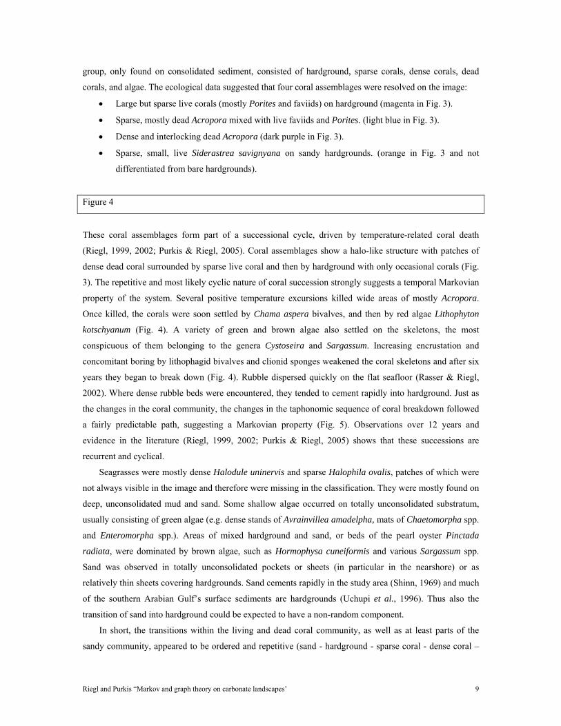
Riegl and Purkis “Markov and graph theory on carbonate landscapes’ 9
group, only found on consolidated sediment, consisted of hardground, sparse corals, dense corals, dead
corals, and algae. The ecological data suggested that four coral assemblages were resolved on the image:
• Large but sparse live corals (mostly Porites and faviids) on hardground (magenta in Fig. 3).
• Sparse, mostly dead Acropora mixed with live faviids and Porites. (light blue in Fig. 3).
• Dense and interlocking dead Acropora (dark purple in Fig. 3).
• Sparse, small, live Siderastrea savignyana on sandy hardgrounds. (orange in Fig. 3 and not
differentiated from bare hardgrounds).
Figure 4
These coral assemblages form part of a successional cycle, driven by temperature-related coral death
(Riegl, 1999, 2002; Purkis & Riegl, 2005). Coral assemblages show a halo-like structure with patches of
dense dead coral surrounded by sparse live coral and then by hardground with only occasional corals (Fig.
3). The repetitive and most likely cyclic nature of coral succession strongly suggests a temporal Markovian
property of the system. Several positive temperature excursions killed wide areas of mostly Acropora.
Once killed, the corals were soon settled by Chama aspera bivalves, and then by red algae Lithophyton
kotschyanum (Fig. 4). A variety of green and brown algae also settled on the skeletons, the most
conspicuous of them belonging to the genera Cystoseira and Sargassum. Increasing encrustation and
concomitant boring by lithophagid bivalves and clionid sponges weakened the coral skeletons and after six
years they began to break down (Fig. 4). Rubble dispersed quickly on the flat seafloor (Rasser & Riegl,
2002). Where dense rubble beds were encountered, they tended to cement rapidly into hardground. Just as
the changes in the coral community, the changes in the taphonomic sequence of coral breakdown followed
a fairly predictable path, suggesting a Markovian property (Fig. 5). Observations over 12 years and
evidence in the literature (Riegl, 1999, 2002; Purkis & Riegl, 2005) shows that these successions are
recurrent and cyclical.
Seagrasses were mostly dense Halodule uninervis and sparse Halophila ovalis, patches of which were
not always visible in the image and therefore were missing in the classification. They were mostly found on
deep, unconsolidated mud and sand. Some shallow algae occurred on totally unconsolidated substratum,
usually consisting of green algae (e.g. dense stands of Avrainvillea amadelpha, mats of Chaetomorpha spp.
and Enteromorpha spp.). Areas of mixed hardground and sand, or beds of the pearl oyster Pinctada
radiata, were dominated by brown algae, such as Hormophysa cuneiformis and various Sargassum spp.
Sand was observed in totally unconsolidated pockets or sheets (in particular in the nearshore) or as
relatively thin sheets covering hardgrounds. Sand cements rapidly in the study area (Shinn, 1969) and much
of the southern Arabian Gulf’s surface sediments are hardgrounds (Uchupi et al., 1996). Thus also the
transition of sand into hardground could be expected to have a non-random component.
In short, the transitions within the living and dead coral community, as well as at least parts of the
sandy community, appeared to be ordered and repetitive (sand - hardground - sparse coral - dense coral –

Riegl and Purkis “Markov and graph theory on carbonate landscapes’ 10
dead coral – rubble – hardground – sparse coral – etc.), thus suggesting the presence of the Markovian
property. Since these components made up the landscape, it was also evident that the steps in the ecological
and taphonomic succession should have an associated landscape expression.
Given that the observations suggested directed and probabilistic transitions among states, discrete
mathematical tools were used to model landscape dynamics: graphs allow visualization of pathways, and
Markov models allow quantification of transition dynamics.
To understand the structure of the classified map, neighbourhood relationships were extracted and a
transition frequency matrix (TFM) was obtained. Via division by row totals, the transition frequency matrix
was transformed into the observed transition probability matrix (TPM) of likelihoods of facies transitions
(Fig. 5 A) from which a weighted digraph was obtained (Fig. 5 B). On the graph, vertices had in- and
outdegrees (referring to the number of facies that either transit into each facies=indegree, or into which it
transits=outdegree) between 4 and 6. The graph had an overall frequency of d=1, since every vertex could
reach another vertex (or itself) in a minimum of one single step. The presence of self-loops made d=1 a
necessary condition (Kemeny & Snell, 1960), which was further proven by a single eigenvector of
magnitude unity (Cox & Miller, 1965).
An expected TPM was calculated from the observed TPM and with a Chi-square test significance of
differences between the matrices was evaluated. The significant differences (p<0.001) confirmed the
presence of the simple Markov property. The expected TPM was raised to higher powers (up to the fifth)
and again the observed against the expected TPM was tested for higher-order Markov property with Chi-
square tests that were significant (p<0.001). Since pixel-size would exert strong control on any higher order
Markov property, (the smaller the pixel and the bigger the patches, the higher the order), this was not
investigated further. To account for pixel-size effects, the matrix was also treated as embedded Markov
chain not allowing self transitions and the Markov property was found again (Chi-square test, p<0.05).
Figure 5
Clearly, the quantitative expression of the spatial facies neighbourhood pattern in the Arabian Gulf was
a regular Markov chain (d=1, higher powers of the matrix without zero entries). From this, a fixed
probability vector was found (Kemeny & Snell, 1960; Horn, 1975; Roberts, 1976) because if n is a row
vector and P is the s x s transition matrix, n(t+1) = n(t).P, and after m generations n(t+m)=n(t).Pm. As m
increases, n converges to a stable distribution, the fixed probability vector n*, which is the solution of s
linear equations n* = n*. P.
The fixed probability vector (FPV) expresses the likelihood with which every state is encountered
independent of the state the Markov chain is started in (Roberts, 1976). If the fixed probability vector
expresses the likelihood of successional stages occurring in space, it could also express their likelihood of
occurring through time. If a point is twice as likely to fall within stage A (or facies A), because A is twice

Riegl and Purkis “Markov and graph theory on carbonate landscapes’ 11
the size of stage (facies) B (to be precise: stage A’s spatial expression in facies A is twice the size of stage
B’s spatial expression in facies B), then through time, everything else being equal, a point will also
probabilistically be encountered twice more often in stage (facies) A than in stage (facies) B. The Law of
Large Numbers for regular Markov chains defines the FPV as representing the fraction of time that the
process can be expected to be in state sj for a large number of steps (Kemeny & Snell, 1960). From this we
propose that the spatial transitions in any landscape could be useful as a proxy for the temporal transitions
and vice versa.
If this were indeed so, the frequency of the facies (which is equivalent to the number of transitions into
and within a facies) visible in the horizontal modern landscape should be at least roughly matched by the
frequency of facies seen in outcrop, provided we were able to find equivalent modern and fossil systems
that are time-transgressive (i.e. comparable environments. It would be nonsensical to compare
environments that do not have similar spatial or ecological dynamics). So, if our conjecture was true that
the FPVs of ancient and modern vertically and horizontally evaluated sedimentologically similar systems
can be similar, we should find similar transitions and total facies frequencies both in the Fenk quarry and
the Arabian Gulf satellite image.
Figure 6
Several caveats have to be applied to this analysis. First of all, not all facies co-ocurred in the Recent and
the fossil landscapes, although many did: dense corals (fossil equivalent: coral framestone) and sparse
corals (fossil equivalent: coral/oyster floatstone, coral rudstone), as well as the sandy facies (Arabian Gulf:
sand, algae, seagrass; fossil equivalent: corallinacean calcarenite). No equivalents existed in the modern
Arabian Gulf for the Isognomon oyster banks, which acted as hardgrounds for coral settlement (the only
equivalent would be Pinctada radiata oyster beds within the Arabian Gulf algae facies, however, the
Recent oysters are much smaller than those of the Miocene) and the rhodolith facies (rhodoliths were
uncommon in the Recent study area). It was possible to directly compare the percent contribution of the
following facies: dense coral (Miocene: framestone, Recent: dense live and dense dead coral), sparse coral
(Miocene: coral rud- and floatstones; Recent: sparse corals), sandy facies (Miocene: corallinacean
calcarenite, Recent: hardgrounds, sand). Other facies correlated approximately, i.e. the Miocene Isognomon
oysterbeds were included into the hardgrounds because their dense shell-layers acted as hardground and
substrate for coral framework initiation. The Miocene marls could be compared (with some liberty) to the
Recent seagrass beds which usually occurred on mud or muddy sand.
Also sampling intensity of the outcrop and grid-size of the two-dimensional outcrop map is of equal
importance as pixel-size in the landscape. We sampled the image at 10 cm intervals (image gridded to 10
cm pixels), since no significant differences (ANOVA, F=2.43, df:5,42, p>0.05) existed between the FPVs
obtained from sampling at 50, 20, 10, 5 and 2 cm. Since we counted the transitions in the Moore
neighbourhood of each pixel, increased within-facies (self-) transitions were balanced by equally increased

Riegl and Purkis “Markov and graph theory on carbonate landscapes’ 12
among-facies transitions. More vertical pixels mean more within-facies self-transitions, but more horizontal
pixels also mean more among-facies transitions in vertically stacked sequences. For this specific section of
the analysis, we were not primarily interested in how the transition probabilities would change with
sampling intensity, but rather whether the chosen sampling intensity would provide a robust-enough FPV
that would allow unbiased comparison with the living Arabian Gulf landscape (i.e. one that would not
change with relatively minor gridding alterations). Since a wide range of sampling intervals did not
significantly change the FPV, our analysis was considered acceptable and we used a 10 cm grid.
The TPM and digraph of the Leitha Limestone are shown in Fig. 7 and Fig. 8. The FPVs (= relative
frequency of facies in the Recent Arabian Gulf and Miocene Leitha Limestone) indeed coincide where the
facies are compatible. No significant differences existed between Recent and Miocene distribution (t-test,
p<0.001, after it tested positively for normality).
Figure 7
The space-time bridge
Based on Fig. 7, the patterns of spatial and temporal facies successions (encapsulated in relative facies
frequencies as expressed by the FPV) were, at least in the chosen example, very similar. To create a model
of how facies transitions work in time and to evaluate resulting facies frequencies if transition probabilities
were changed, either the vertical or the horizontal transition matrix could be chosen for the construction of
the model. Because of better control and more information about the living spatial structure, the Recent
landscape was chosen to start with. A temporal transition digraph was constructed from the spatial
adjacency digraph by modifying in- and outdegrees whenever certain transitions were only possible in
space but not in time (or vice versa, if one wanted to use the temporal transitions to model spatial
transitions). For example, sand may directly neighbour dense coral horizontally and vertically (Fig. 5 B),
but a successional transition from sand directly into dense coral is not possible in a single step. Rather, sand
has to first pass through hardground and sparse coral stages (Fig. 8 A, B).
Constraints for the temporal Markov model were: (1) use of the same vertices (facies) in the temporal
digraph (matrix) as in the spatial digraph (matrix) (2) maintenance of the same number of vertices (=
facies). Accuracy of the derived model was assessed by (3) the FPV, which defines the likelihood of facies
encounter irrespective of starting state. Therefore, differences between the FPV from the temporal digraph
(matrix) and the actually observed size distribution of stages or facies obtained by pixel-counting the
classified satellite image should not be significant. The FPV of the temporal TPM should correspond with
the FPV of the horizontal (living, landscape) and vertical (ancient, outcrop) TPMs.
If either the temporal or spatial model was assumed to be more complex than the other, then conditions
(1) and (2) could be relaxed to let the same vertices (facies) occur but to allow additional vertices (facies) in
the matrix and FPV. The corresponding FPVs had to conform to (3), i.e. not differ in corresponding facies.
In such a case, differences between vectors could not be tested for significance due to different size.

Riegl and Purkis “Markov and graph theory on carbonate landscapes’ 13
In the case of the Arabian Gulf biostrome, the spatial model was expressed by a regular Markov chain
with eight vertices and d=1 (Fig. 5 B). Each vertex could be reached by every neighbour (or itself) in one,
or any multiple of one, steps. Translated into time, this would assume total reversibility of any process.
However, this is known not to be the case in many ecological and sedimentological processes. The FPV
only informs about the proportional share of each state’s ni occurrence. To transform the matrix of spatial
adjacencies into an ecologically and sedimentologically meaningful model of system functioning in time,
we had to take some liberties.
The digraph of spatial transitions (Fig. 5 B) showed the two previously demonstrated functional groups
in the Arabian Gulf (Fig. 3) and the Fenk outcrop: unconsolidated facies (sand and everything that grows
on sand, in our case algae and seagrass) and consolidated facies (hardground and everything that grew on it,
like algae, the coral biostrome and its degradation products such as dead corals and corals covered by
algae). Within the unconsolidated facies, sand was considered as a central node from which seagrass and
algae, that also transited into each other, could be reached. This was based on observations of seagrass
interweaved with dense algae fluctuating in time and space. The treatment of sand and its transition into
hardground was key in defining the nature of the model. It is known (Shinn, 1969; Uchupi et al., 1996) that
sand in the southern Arabian Gulf rapidly cements into hardgrounds due to the high alkalinity of the
seawater. Once consolidated, the sand turns to rock and will not return to sand in any appreciable quantity,
with the exception of parts that get ground-up to sand in higher-energy environments. Thus, in an
imaginary core through this landscape, consolidated sand will forever remain consolidated sand, since any
cover by mobile sand sheets would not be detectable in the geologic record. But in the active landscape,
hardground can very well be covered by sand and in the spatial digraph (Fig. 5 B) there is a strong (i.e.
bilateral) connection. This suggested two treatments: first considering the transition sand-hardground
reversible with the argument that when a patch of hardground is covered by sand it is functionally sand and
can revert to hardground when the sand is removed, in which case the Markov chain remains regular. This
could be considered a more biological line of argument since sand cover will make habitat unsuitable for
fauna and flora that require hardground. Second the transition sand-hardground could be considered
irreversible (the “geologic” line of argument, because even if covered by a layer of sand, the hardground
itself remains hard), which makes the Markov chain ergodic and the transient unconsolidated sediments
eventually get absorbed into the hardground-coral set. This allows exploration of two Markov models: one
regular, one ergodic.
Figure 8
When constructing the TPM of temporal dynamics in the regular model, we reordered the sequence of
vertices to make the system easier to understand (Fig. 9). The resulting matrix consisted of four
submatrices: the ‘unconsolidated’ facies (B2) in the lower right, the ‘consolidated facies’ in the upper left
(B1), transitions from B2 into B1 in the upper right (B12), and transitions between the upper left and lower
Riegl and Purkis “Markov and graph theory on carbonate landscapes’ 14
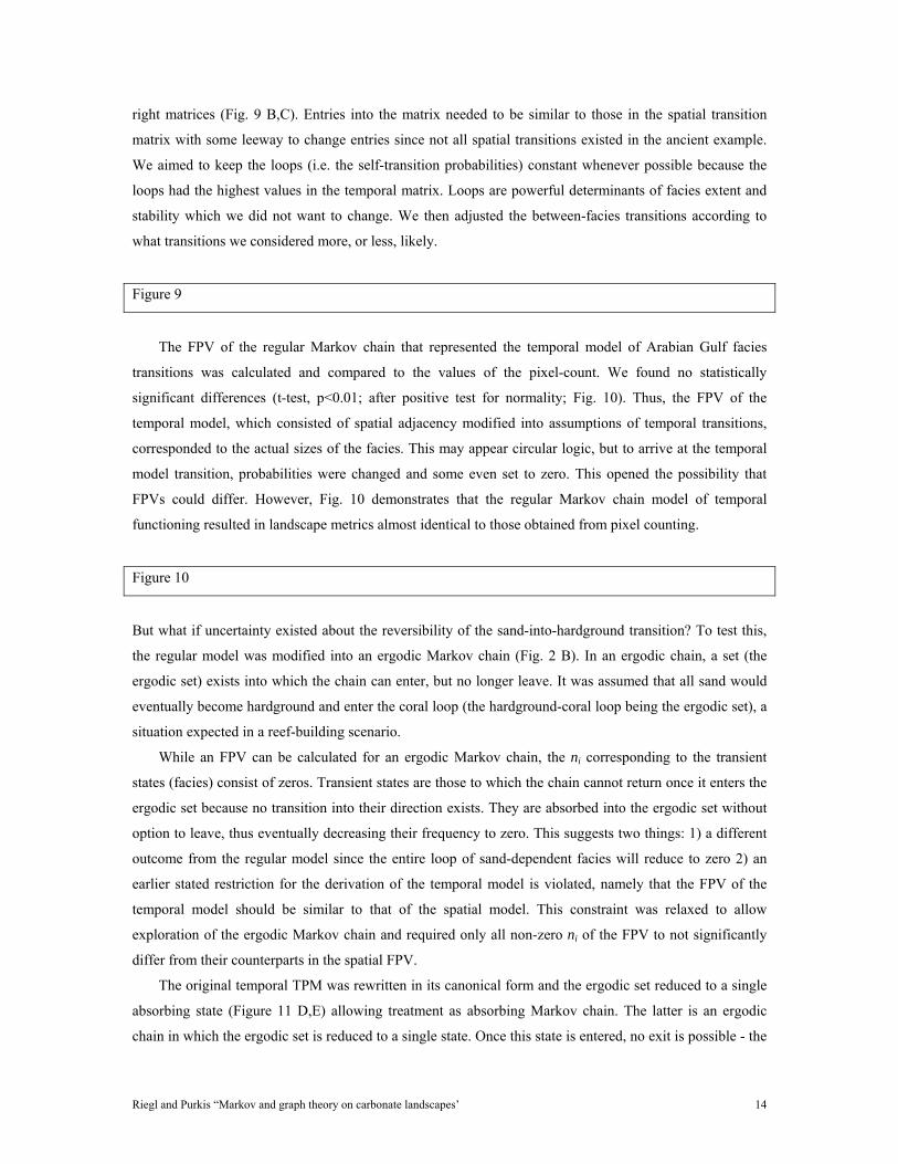
right matrices (Fig. 9 B,C). Entries into the matrix needed to be similar to those in the spatial transition
matrix with some leeway to change entries since not all spatial transitions existed in the ancient example.
We aimed to keep the loops (i.e. the self-transition probabilities) constant whenever possible because the
loops had the highest values in the temporal matrix. Loops are powerful determinants of facies extent and
stability which we did not want to change. We then adjusted the between-facies transitions according to
what transitions we considered more, or less, likely.
Figure 9
The FPV of the regular Markov chain that represented the temporal model of Arabian Gulf facies
transitions was calculated and compared to the values of the pixel-count. We found no statistically
significant differences (t-test, p<0.01; after positive test for normality; Fig. 10). Thus, the FPV of the
temporal model, which consisted of spatial adjacency modified into assumptions of temporal transitions,
corresponded to the actual sizes of the facies. This may appear circular logic, but to arrive at the temporal
model transition, probabilities were changed and some even set to zero. This opened the possibility that
FPVs could differ. However, Fig. 10 demonstrates that the regular Markov chain model of temporal
functioning resulted in landscape metrics almost identical to those obtained from pixel counting.
Figure 10
But what if uncertainty existed about the reversibility of the sand-into-hardground transition? To test this,
the regular model was modified into an ergodic Markov chain (Fig. 2 B). In an ergodic chain, a set (the
ergodic set) exists into which the chain can enter, but no longer leave. It was assumed that all sand would
eventually become hardground and enter the coral loop (the hardground-coral loop being the ergodic set), a
situation expected in a reef-building scenario.
While an FPV can be calculated for an ergodic Markov chain, the ni corresponding to the transient
states (facies) consist of zeros. Transient states are those to which the chain cannot return once it enters the
ergodic set because no transition into their direction exists. They are absorbed into the ergodic set without
option to leave, thus eventually decreasing their frequency to zero. This suggests two things: 1) a different
outcome from the regular model since the entire loop of sand-dependent facies will reduce to zero 2) an
earlier stated restriction for the derivation of the temporal model is violated, namely that the FPV of the
temporal model should be similar to that of the spatial model. This constraint was relaxed to allow
exploration of the ergodic Markov chain and required only all non-zero ni of the FPV to not significantly
differ from their counterparts in the spatial FPV.
The original temporal TPM was rewritten in its canonical form and the ergodic set reduced to a single
absorbing state (Figure 11 D,E) allowing treatment as absorbing Markov chain. The latter is an ergodic
chain in which the ergodic set is reduced to a single state. Once this state is entered, no exit is possible - the

Riegl and Purkis “Markov and graph theory on carbonate landscapes’ 15
chain is “absorbed” into it. From the canonical matrix “landscape drift” (in analogy to the “ecological drift”
of Hubbell (2001)) was calculated, which is the number of times the system resides in any transient state
(facies) sij before absorption:
N = (I-Q)-1,
where I is the absorbing matrix (an identity matrix of the appropriate dimension corresponding to Q)
and Q is the matrix of transient states. ξ is a column vector of ones and the fixation times (the time until
absorption – where time is measured in matrix steps) were calculated as
τ(N) = Nξ , with a variance of Var(τ) = (2N-I)τ-τsq ,
where τsq contains all values of τ squared. And, finally,
B = N.R
where N is the fundamental matrix and R the matrix of transient states gives the likelihood of absorption
(which is known to be 1, because the transient states reduce to zero in the FPV).
In analogy to what was done to obtain Fig. 10, the FPV was calculated (Fig. 11 G). Compared to the
values of the regular temporal model and the spatial matrix, the outcome was obviously different. Due to
absorption, no soft substrata remained and all time was spent in the hardground/coral loop. This would be
equivalent to reefbuilding dynamics, in that all free substratum would be eventually converted into
hardground on which corals would settle that would then proceed to grow generation on top of generation
to form a bioherm. This obviously was not the case in the study area, where only biostromal frameworks
(single-generation frameworks) or non-framework communities were found. Thus, the ergodic/absorbing
model did not conform to reality and was rejected. This process demonstrated that simply using the same
vertices as in the spatial adjacency matrix and adjusting transitions did not automatically lead to a temporal
model that would produce plausible results.
Facies pattern and environmental change - Landsat image analysis Arabian Gulf
If it is predicted that the vertical and/or horizontal transitions can be used to build a model of
sedimentary system functioning, then it should also be possible to make fore- or hindcasts regarding a
system’s state in different environments. These changes could be represented by modifying the
probabilities of facies transitions (i.e. the weightings of edges).
To explore this further, a shoal system at Murrawah and Al Gharbi on the Great Pearl Bank was
studied using Landsat imagery (Fig. 12). Only areas of < 8 m water depth were classified, since waters had
a relatively high particulate load and therefore did not allow adequate light penetration for remote
distinction of facies deeper than that. Deeper facies in the Arabian Gulf tend to be primarily sandy. Eight
bottom types could be delineated. Murawwah, Al Gharbi, Al Hila and Fiyya islands were surrounded by
shallow, partly emergent sands (dark purple) that also occurred on the shallowest parts of the banks. The
shallow subtidal parts of the banks were covered by mobile submerged sand and muddy sand sheets (light
blue), submerged at low tides. Deeper (<2m) parts were covered by sparse seagrass (mainly Halophila spp.

Riegl and Purkis “Markov and graph theory on carbonate landscapes’ 16
and Halodule uninervis) and algae (yellow) on sand. Dense seagrass meadows, consisting of tall Halodule
uninervis were found towards the edges of the shoals (blue), seaward of which dense algae meadows
occurred (green), consisting primarily of brown algae (Hormophysa cuneiformis, Sargassum spp.,
Cystoseira spp.). Much of the platform was surrounded by a fringe of coral biostromes (dark blue). In the
center-left of Fig. 13 (just above the text ‘Murawwah Island’) is a series of stringer-shaped bioherms partly
with algae cover.
Fig. 11
Fig 12
The position of the bottom classes relative to each other and the shoals suggested, in particular for the
biofacies, dependence on position on the bank and water depth. The simple Markov property was present in
adjacencies (Chi-square test p<0.001). The weighted digraph of the TPM is illustrated in Fig. 13 B and
shows vertices with in- and outdegrees between 1 and 5, a frequency of d=1. We encountered a regular
Markov chain.
Fig. 13
Using the approach developed earlier in this paper, little modification was needed to change the spatial
matrix into a temporal transition matrix. The spatial model was a regular Markov chain with six vertices
and d=1. Translated into time, this would assume reversibility of any process and would suggest that these
facies can all easily transit into each other, even take each other’s place depending on transition weightings.
The boundary to the deep water facies that were not evaluated because they were beyond the optical
resolution of the Landsat image, was coral. The shallow boundary was formed by emergent sand.
All vertices (facies) had strong loops (transitions to themselves, Fig. 13) suggesting that pixels in the
image classes encoding these vertices (facies) were most frequently adjacent to pixels of the same class, i.e.
they formed large, contiguous patches with a low outline/volume ratio. We surmise that what is true in
space may also be true in time. Both coral and seagrass/algae can be relatively stable on the short,
ecological time-scale operating in decades to few centuries. Transition from coral into dense algae occurs
when corals die and are overgrown by algae. The coral die-back events on decadal scales lead to higher
transition probabilities from corals to dense algae than any other facies. Similar directed temporal
transitions would occur between dense seagrass/algae and sparse seagrass/algae whenever conditions are
unfavorable (extreme hot or cold events, changes in sea-level) and between the latter and bare sand sheets.
By changing transition likelihoods in the temporal TPM, we examined how the distribution of facies
might change and basic predictions were made about effects of a changed environment, in this case sea-
level rise and fall of 1.5 to 2 m. This gentle oscillation remained within the relatively narrow depth range

Riegl and Purkis “Markov and graph theory on carbonate landscapes’ 17
over which facies were evaluated on the Landsat image (0-8 m). Sea-level was treated implicitly and the
bathymetric information did not enter into any calculation - water got “shallower” or “deeper”. So if sea-
level was considered to rise, a transition into a deeper facies could be expected in previously shallow areas.
Thus the transition probability shallow-to-deep-facies had to be increased. To simulate rises or falls in sea-
level, we modified transitions between facies thus allowing preferential changes into facies that might be
better adapted to the new environment, defined by water depth. Fig. 14 outlines the directions of anticipated
changes and the fixed-point vectors of the modified TPM (Fig. 14 B, C, Fig. 15), allowing to predict future
distribution of facies. To generate the model, the sum of all loop-values (probabilities of self-transition)
was kept constant. Then the loop values of those vertices (facies) that were assumed to shrink in the
changed environment were rounded down to the next integer decade (10, 20, 30, etc.). The amount that had
been gained by rounding-down the loops was then re-distributed over those vertices (facies) that were to be
at an advantage in the changed environment causing stronger retention in these facies. Transitions between
facies were adjusted to respect the constraint of row summability to unity. Depending on the environmental
change desired, the transition probabilities into either the neighbouring shallower or deeper facies was
increased, while transitions into facies at the same depth were kept at equal weight. This had the effect that
either the facies at the shallow extreme (emergent sand) or deep extreme (dense coral) became more
reflecting (in the sense that the chain would not transit frequently into and remain long at the extremes, thus
their frequency in the FPV would be decreased) or more absorbing (in the sense that the extremes would be
more frequently transited into and the chain would remain longer in them, increasing their frequency in the
FPV). Thus it was possible to let facies adjust in frequency at the cost of each other, depending on how sea-
level would position them on the gently changing depth ramp and whether they encountered their preferred
depth range. Since the system was bounded at the shallow and the deep ends due to the nature of the
analysis (masking of pixels deeper than dense corals) and limited space was available on the banks for
changes in facies composition, no new facies could be generated.
Fig. 14
In the rising sea-level scenario (facies transit preferentially into a neighbouring deeper-water facies,
shown in Fig. 14 by fat arrows), the shallow facies (emergent sand, submerged sand, sparse seagrass/algae)
were made to retreat strongly (Fig. 15) and the facies typically found on the bank-edges (corals, dense
algae) increased due to better availability of habitat in their preferred depth range. This is plausible since
little space exists for a landward retreat of shallow facies (the islands are not that big) and the gently
sloping edges of the platform will provide much suitable new habitat for algae and corals without much
habitat loss due to drowning. Emergent sand would be flooded and colonized by algae and seagrass. The
newly flooded areas of formerly dry land (the islands) would become shallow, at least partly emergent
sand. In the falling sea-level scenario, emergent and shallow subtidal sands would greatly expand at the
cost of the deeper facies, which would move into yet deeper areas (masked pixels) and maybe decline less

Riegl and Purkis “Markov and graph theory on carbonate landscapes’ 18
dramatically than illustrated in Fig. 15. However, since the deeper, masked areas were not included in the
analysis, a precise numeric evaluation was not possible. Within the 0-10 m depth zone the decline was
adequately represented (Fig. 15).
Fig. 15
DISCUSSION
We have explored a computationally and conceptually simple way of harnessing spatial patterns in a
landscape to extrapolate information for modifying spatial into temporal transitions. Markov chains and
weighted digraphs provided the opportunity to forecast changes in facies by manipulating transition
likelihoods obtained from lateral patterns in a living landscape. This allows translating knowledge of facies
transitions in core or outcrop (=time) for the reconstruction of ancient landscapes (=space) and vice versa
(Doveton 1994; Parks et al., 2000; Elfeki & Dekking 2001, 2005) and the frequency of facies that can be
expected in any time slice. Thus, we can improve for example the estimation of the lateral dimensions of
reservoir rocks. Our study also builds on and expands the concepts developed in Lehrmann & Rankey
(1999), who showed the value of incorporating knowledge of lateral facies extension in outcrop to obtain
improved understanding of cyclicity.
The investigated sedimentary systems were characterized by facies of fairly uniform thickness for
which we assumed comparable sedimentation rates, thus no rate-adjustments were made for translations
from space into time and vice versa. Differential sedimentation rates and their realization in Markov chains
are discussed by Parks et al. (2000) who scaled transitions by a constant relative to sedimentation rate
(Schwarzacher, 1969). Bioherms, for example, may accrete faster vertically rather than laterally, and faster
than surrounding sediments. Such a situation would lead to a stronger self-transition (loop) in the vertical
than the lateral. Additional to the method of Parks et al. (2000), the use of embedded Markov chains would
also be useful since these ignore the self-transitions that encode within-facies deposition rate. However,
such an analysis would limit itself to evaluating adjacencies and loose any information contained in the
loops. Coral frameworks investigated in this paper were mostly biostromal (i.e. coral carpets sensu Riegl &
Piller, 2000), thus not accreting faster to much greater thickness than surrounding sediments and no
corrections by loop-multiplication were deemed necessary.
The modern and the Miocene situations explored in our study have in common that both were
evaluated only in a small piece of the entire system - whatever was imaged in the Arabian Gulf and the
relatively small Miocene outcrop. The Ras Hasyan area was described from a 7x1.5 km plane area and the
Leitha Limestone from an outcrop 20m high and 60 m long. This difference in scale and the obvious
incompleteness with regards to the entire landscape need not matter since first we were uniquely interested
in the relative frequency of facies and second the living Arabian Gulf landscape has fractal properties
(Purkis et al., 2005). The correspondence of the FPVs of Miocene and living Arabian Gulf system may

Riegl and Purkis “Markov and graph theory on carbonate landscapes’ 19
suggest that, since the Miocene system was very similar (Riegl and Piller, 2000), it may also have been
fractal. Therefore, the different sizes of study areas may indeed be of no importance. Different outcrop or
map scales simply will detect patches of different sizes but in comparative proportion. Thus, in the
illustrated case here, we believe that both systems were similarly patterned in space and therefore the fixed-
point vector as the bridge between space and time would hold at all scales and between scales. This would
relieve us of the need to compare landscapes and successions of comparable sizes. In our study, facies were
at best several meters thick and a small outcrop of few hundred square-meters could be plausibly
interpreted as accommodating a comparable number of facies (bearing in mind that the assignment of facies
always remains somewhat subjective) as the moderately large modern study area of about 70 km2.
Difficulties may arise when estimating facies of vastly varying thickness, as would be expected to be
caused by variable deposition rates. While the assumption of the fractal nature of the landscape may still
hold, care would be needed to assure sampling at appropriate scales – which would have to be evaluated
using spatial statistics.
Transition weightings between facies depend strongly on environmental factors and a complex
interplay exists between ecology and sedimentology. When deriving our temporal facies models from the
spatial adjacencies, we were strongly guided by the ecology of facies-determining organisms (coral, algae,
seagrass) to decide which transitions were possible. In particular, the dynamics of the corals, as producers
of bioherms, biostromes or rubble in the Recent Arabian Gulf and the Miocene Leitha Limestone, strongly
influenced the sedimentology by producing well-defined biofacies that were directly equivalent to
sedimentary facies. Algae and seagrass interacted with the sedimentary environment in a more passive way,
presumably primarily as binders and bafflers. However, simply their presence and cover of unconsolidated
sediments would to a certain extent protect the latter from erosion, thus giving them sedimentological
relevance. Their clear ecological preferences and distribution on the banks made them useful indicators for
facies on the satellite images and proxies in the models. Dense algae clearly was found primarily on the
grainstone-dominated platform edges and as secondary cover on dead coral frameworks, while dense and
sparse seagrass was found primarily on the finer-grained bank interior (Purser, 1973; Schlager, 2005).
An obvious key environmental factor with the potential of shaping facies distribution is the depth of
the water column through which light, thermal and wave energy transit to the benthic biota and sediments.
The importance of small-scale sea-level oscillations and their influence on the distribution of facies in
shallow water is a matter of active debate (Lehrmann & Goldhammer, 1999; Rankey, 2004; Burgess,
2006). We introduced directional changes in the facies transition likelihoods to simulate sea-level, and
obtained via the fixed probability vector the expected distribution of facies in a new environment. Such
thought-experiments have the potential of increasing our understanding of both lateral as well as vertical
facies succession, however, they are only valid if the facies can indeed realistically transit into each other.
In our study area, a relatively mild depth gradient was observed (Fig. 15 D) with the potential of facies
moving relatively unhindered up and down the bank and expanding or shrinking at each other’s expense in
response to a small change in sea-level. Other than eustatic, such changes could be caused by gentle

Riegl and Purkis “Markov and graph theory on carbonate landscapes’ 20
subsidence and subsequent filling of accommodation space. If seen from this perspective, our model could
be used as a quantitative analogue to Ginsburg-type autocyclic sedimentation (Ginsburg, 1971; Hardie &
Shinn, 1986; Schlager, 2005).
As can be expected in an offshore bank setting, shallow and nearshore facies became more and more
limited in area in the rising sea-level scenario, and in the falling sea-level scenario the shallow infratidal
and the deeper facies became restricted. This disadvantage of deeper facies was caused by the model not
considering seafloor > 8 m. Interestingly, this depth is the boundary between typical high light/shallow and
low light/deeper biota and sedimentary environments in the Recent Arabian Gulf. Yet by masking, we
created an artificial lower boundary that need not exist. Facies occurring in deeper water could simply
move down–slope and therefore not require as markedly increased reflection (translated into decrease of
facies extent) at the lower boundary as in our model. However, since our bathymetric information was
derived from the same satellite image as the information about facies, it was limited to the same depth and
we resisted speculation on what lay beyond. In particular, slope geometry will have to be considered when
parameterizing such models, since it will define how facies can migrate up or down while tracking sea-
level. Any cycles generated from such a Markov model would be necessarily non-random and while it
would be a good tool to model landscapes from cores and vice versa, it would not be an adequate forward
modelling tool for questions of order and noise in sequences (Wilkinson et al., 1997, 2003; Lehrmann &
Goldhammer, 1999; Rankey, 2004; Burgess, 2006).
When using the derived temporal models to predict changes in facies, as we did for the Landsat scene
in rising/falling sea-level scenarios, the fixed probability vector gives information about the contribution of
facies in the new environment but not about the time needed to achieve this. It is possible to evaluate how
many matrix-time steps are needed (i.e. to what power the TPM needs to be raised) until a distribution of
facies close to that of the FPV is obtained. Using an absorbing model, we have shown that it is possible to
calculate time until absorption of the transient facies (Fig. 11). However, the time-scale is always one of
matrix multiplication steps and careful calibration of a matrix step’s meaning in years is required. Such
information could be obtained in outcrop by dating the length of time required for a facies transition
predicted from the spatially-derived model. In our case, we had no cores through the living Arabian Gulf
environment, nor could we obtain reliable dating from the Miocene outcrop and therefore cannot offer time
information. Clearly more work on this aspect is required.
The depth of sea-level fall and height of sea-level rise needs to be encoded in the transition
probabilities. In our case, assumptions of sea-level rise and fall were small, in the range of 1.5-2 m. The
biological, and to some degree the sedimentary environments encountered on the studied banks are
relatively sensitive depth indicators and occurred within relatively specific depth ranges (Figs 3, 12).
Therefore, they could expand and restrict at the cost of each other and no new facies had to be introduced.
Models as we presented, are limited to situations without dramatic changes in facies arrangement and
composition and require at least a certain facies-depth relationship, which is not always unequivocal
(Rankey, 2004).

Riegl and Purkis “Markov and graph theory on carbonate landscapes’ 21
The application of Markov chains to sedimentary systems or to ecological succession is not new
(Krumbein, 1967; Schwarzacher, 1969; Pielou, 1969; Horn, 1975; Usher, 1979), and its conceptual link to
Walther’s Law for the forward modelling of sedimentary landscapes has also been noted before (Doveton
1994; Parks et al., 2000; Elfeki & Dekking, 2005). What is new in our analysis is the addition of graphs for
the easy visualization of functional pathways within the system and derivation of a spatial model from the
temporal - or vice versa. This allows ecology and sedimentology to be linked, since heed can be paid to
ecological dynamics that may need to be introduced into the derived models of facies dynamics via
modified transition probabilities. This is the important new step to the existing techniques used for forward
modelling with Markov chains – the visualization of spatial relationships and the derived temporal
functioning in graphs. Rather than adapting the transition matrix via weightings by scaling factors
(Schwarzacher, 1969; Parks et al., 2000) the graph-evaluation step allows a quite realistic derivation of a
temporal matrix (or spatial matrix, depending on starting point) from the spatial matrix. The fixed point
vector is the link between the spatial and temporal models and any modification must result in statistically
similar FPVs. This essentially makes the fixed point vector a quantitative expression of Walther’s Law and
the unifying link between (matrix - and thus its encoded facies) space and time.
ACKNOWLEDGEMENTS
We thank R. N. Ginsburg for being an inspiration and an enthusiastic as well as patient teacher. He planted
more ideas in our minds than we ourselves are aware of. He taught us how to think, ask questions, and keep
an open, yet critical, mind. His contribution to our science is unrivalled. And by making us ask the “so
what?” question after every major thought or posit, he made us go and think further and better than we
would have otherwise. Work on this paper was sponsored among others by the Austrian Science
Foundation (FWF), Austrian Geological Survey, the Dolphin Energy/WWF Coral Reef Project, the Ocean
Drilling Project and NOAA grant NA16OA1443 to NCRI at NSU. E. Rankey contributed many useful
thoughts, discussions and carefully edited the manuscript. W. E. Piller helped with measured sections and
evaluating the Fenk outcrop. We thank M. Chandler, G. Rae, R. al Mubarak, Th. Abdessalaam, A. al
Cibahy and F. Launay for unwavering support during work in the Gulf. This is NCRI publication #84 and a
contribution of the NCRI Monitoring Network.
REFERENCES
ALSHARHAN, A.S. & KENDALL, C.G.C. (2003) Holocene coastal carbonates and evaporites of the southern
Arabian Gulf and their ancient analogues. Earth Sci. Reviews, 61 (3-4), 191-243.
BERGGREN, W. A., KENT, D. V., FLYNN, J. J. & VAN COUVERING, J. A. (1985) Cenozoic geochronology.
Geol. Soc. Am. Bull., 96, 1407-1418.

Riegl and Purkis “Markov and graph theory on carbonate landscapes’ 22
BUNN, A.G., URBAN, D.L., & KEITT, T.H. (2000) Landscape connectivity: a conservation application of
graph theory. J. Environ. Manag., 59, 265-278.
BURGESS, P.M. (2006) The signal and the noise: Forward modelling of allocyclic and autocyclic processes
influencing peritidal carbonate stacking patterns. J. Sed. Res., 76, 962-977.
CANTWELL, M.D., & FORMAN, R.T.T. (1993) Landscape graphs: Ecological modeling with graph theory to
detect configurations common to diverse landscapes. Landscape Ecology, 8, 239-255.
CARLE, F.S., & FOGG, G.E. (1997) Modeling spatial variability with one and multidimensial continuous-lag
Markov chains. Mathematical Geology, 29, 891-918.
CASWELL, H. (1982) Stable population structure and reproductive value for populations with complex life
cycles. Ecology, 63, 1223-1231.
CASWELL, H. (2001) Matrix population models. Sinauer Associates, Sunderland, 722 pp.
COX, D.R., & MILLER, H.D. (1965) The theory of stochastic processes. John Wiley and Sons, New York,
422 pp.
DAVIS, J.C. (2002) Statistics and data analysis in Geology. 3rd Edition, John Wiley and Sons, New York,
637 pp.
DOVETON, J.H. (1971) An application of Markov chain analysis to the Ayreshire coal measures succession.
Scott. J. Geol., 7, 11-27.
DOVETON, J.H. (1994) Theory and application of vertical variability measures from Markov chain analysis.
Computer applications in geology 3 (Eds J.M. Yarus J.M. and A.L. Chamberlain) Am. Assoc.
Petrol. Geol., 55-64.
DULLO, W.C. (1983) Fossildiagenese im miozänen Leitha-Kalk der Paratethys von Österreich: Ein Beispiel
für Faunenverschiebung durch Diageneseunterschiede: Facies 8, 112 pp.
ELFEKI, A. & DEKKING, M. (2001) A Markov chain model for subsurface characterization: theory and
applications. Mathematical Geology, 33(5), 569-589.
ELFEKI, A. & DEKKING, M. (2005). Modelling subsurface heterogeneity by coupled Markov chains:
Directional dependency, Walther’s law and entropy. Geotechn. Geol. Engineering, 23, 721-756.
EVANS, G., MURRAY, J.W., BIGGS, H.E.J., BATE, R., & BUSH, P.R. (1973) The oceanography, ecology,
sedimentology and geomorphology of parts of the Trucial Coast barrier island complex, Persian
Gulf. The Persian Gulf. Holocene carbonate sedimentation and diagenesis in a shallow
epicontinental sea. (Ed B.H. Purser). Springer, Berlin Heidelberg New York, pp. 233-278.
FLÜGEL, E. (2004) Microfacies of carbonate rock. Springer, Berlin, 976 pp.
FRIEBE, J. (1990) Lithostratigraphische Neugliederung und Sedimentologie der Ablagerungen des
Badeniens (Miozän) um die Mittelsteirische Schwelle (Steirisches Becken, Österreich): Jahrb.
Geol. BA, 133, p. 223-257.
FRIEBE, J.G. (1991) Carbonate sedimentation within a siliciclastic environment: the Leithakalk of the
Weißenegg Formation (Middle Miocene, Styrian Basin, Austria): ZB Geol. Paläont., 1, 1671-1687.
GINGERICH, P.D. (1969) Markov analysis of cyclic alluvial sediments: J. Sed. Petrol., 39, 330-332.

Riegl and Purkis “Markov and graph theory on carbonate landscapes’ 23
GINSBURG, R.N. (1957) Early diagenesis and lithification of shallow-water carbonate sediments in South
Florida. - In: Regional aspects of carbonate deposition. - SEPM Spec. Publ., 5, 80-100.
GINSBURG, R.N. (1971) Landward movement of carbonate mud: new model for regressive cycles in
carbonates (abs.). AAPG Bull., 55, 340.
GINSBURG, R.N. (1974) Introduction to comparative sedimentology of carbonates. AAPG Bull., 58(5), 781-
786.
GINSBURG, R.N. ed. (1975): Tidal deposits. A casebook of recent examples and fossil counterparts.
Springer, Berlin, 428 pp.
GINSBURG, R.N., & SHINN, E. (1994) Preferential distribution of reefs in the Florida Reef Tract: The past is
the key to the present. In: Global Aspects of Coral Reefs: Health, Hazards and History (Ed R.N.
Ginsburg). University of Miami Rosenstiel school of Marine and Atmospheric Science, Miami,
21-26.
HARDIE, L.A. & SHINN, E.A. (1986) Carbonate depositional environments, modern and ancient. Part 3 –
tidal flats. Colorado School of of Mines Quart., 80, 74 pp.
HARRIS, P.M., & KOWALIK, W.S. (1994) Satellite images of carbonate depositional settings: examples of
reservoir- and exploration-scale geological facies variation. AAPG Methods in Exploration Series,
11, 147 pp.
HETZINGER, J, HALFAR, J., RIEGL, B., & GODINEZ-ORTA, L. (2006) Sedimentology and acoustic mapping of
modern rhodolith beds on a non-tropical carbonate shelf (Gulf of California, Mexico). J. Sedim.
Res., 76, 670-682.
HORN, H.S. (1975) Markovian properties in forest succession. in. Ecology and Evolution of communities
(Eds M.L. Cody, J.M. Diamond). Harvard University Press, Cambridge Mass. pp. 196-211.
HUBBELL, S.P. (2001) The unified neutral theory of biodiversity and biogeography. Princeton Monographs
in Population Biology: 32, 375 pp.
IOSIFESCU, M. (1980) Finite Markov processes and their applications. John Wiley and Sons, New York
JAMES, N.P. (1984) Shallowing-upward sequences in carbonates. In: Facies models (Ed R.G. Walker)
Geoscience Canada Reprint Series, Kitchener, Ontario, pp. 213-228.
KEMENY, J.G., & SNELL, J.L. (1960) Finite Markov Chains. Springer Verlag, Berlin, 224 pp.
KIRKHAM, A. (1998) A Quaternary proximal foreland ramp and its continental fringe, Arabian Gulf, UAE.
In: Carbonate Ramps (Eds V.P. Wright, T.P. Burchette). Geol. Soc. (Lond.) Spec. Pub., 149, p. 15-
42.
KRUMBEIN, W.C. (1967). FORTRAN IV computer program for Markov chain experiments on geology.
Computer contributions 13, Kansas Geological Survey, Lawrence, Kansas, 38 pp.
KRUMBEIN, W.C. & GREYBULL, F.A. (1967) An introduction to statistical models in geology. McGraw Hill,
New York, 475 pp.
KRUMBEIN, W.C. & DACEY, M.F. (1969) Markov chains and embedded Markov chains in geology. Int.
Assoc. Mathemat. Geol., 1, p. 79-96.

Riegl and Purkis “Markov and graph theory on carbonate landscapes’ 24
LAMBECK, K. (1996) Shoreline reconstructions for the Arabian Gulf since the last glacial maximum. Earth
Planet Sci. Lett., 142, 43-57.
LEHRMANN, D.J. & GOLDHAMMER, R.K. (1999) Secular variation in parasequence and facies stacking
patterns of platform carbonates: a guide to application of stacking pattern analysis in strata of
diverse ages and settings. In: Advances in Carbonate Sequence Stratigraphy: Applications to
Reservoirs, Outcrops, and Models. (Eds. P.M. Harris, A.H. Saller, J.A. Simo). SEPM Spec. Pub.,
63, 51-62.
LEHRMANN, D.J. & RANKEY, E.C. (1999) Do meter-scale cycles exist? A statistical evaluation from vertical
(1-D) and lateral (2-D) patterns in shallow-marine carbonates-siliciclastics of the “fall in” strata of
the Capitan Reef, Seven Rivers Formation, Slaughter Canyon, New Mexico. In: Geologic
Framework of the Capitan Reef. (Eds. A.H. Saller, P.M. Harris, B.L. Kirkland, S.J. Mazzullo)
SEPM Spec. Pub., 65, 51-62.
LOGOFET, D.O. & LESNAYA, E.V. (2000) The mathematics of Markov models: what Markov chains can
really predict in forest successions. Ecol. Modelling, 126, 285-298.
MIALL, A.D. (1973) Markov chain analysis applied to ancient alluvial plain successions. Sedimentology,
20, 347-364.
MIDDLETON, G.V. (1973). Johannes Walther's Law of the Correlation of Facies. Geol. Soc. Am. Bull., 84,
979–988.
PAPP, A., CICHA, I., SENES, J., & STEININGER, F. (1978) M4 – Badenien (Moravien, Wielicien, Kosovien).
Chronostratigraphie und Neostratotypen. Miozän der Zentralen Paratethys: Slowakische
Akademie der Wissenschaften, Bratislava, 594 pp.
PARKS, K.P., BENTLEY, L.R., & CROWE, A.S. (2000) Capturing geological realism in stochastic simulations
of rock systems with Markov statistics and simulated annealing. J. Sed. Res., 70, p. 803-813.
PIELOU, E.C. (1969) An introduction to mathematical ecology. John Wiley and Sons, New York, 245 pp.
PILLER, W.E., & KLEEMANN, K. (1991) Middle Miocene Reefs and related facies in eastern Austria. 1)
Vienna Basin: VI International Symposium on Fossil Cnidaria including Archaeocyatha and
Porifera, Excursion Guidebook, Excursion B4, 1-28.
PILLER, W.E., & VAVRA, N. (1991) Das Tertiär im Wiener und Eisenstädter Becken: in Roetzl, R., and
Nagel, N., eds., Exkursionen im Tertiär Österreichs, Molassezone – Waschbergzone - Korneuburger
Becken - Wiener Becken - Eisenstädter Becken: Österreichische Paläontologische Gesellschaft, 161-
216.
PILLER, W.E., DECKER, K., & HAAS, M. (1996) Sedimentologie und Beckendynamik des Wiener Beckens:
Sediment 96, 11. Sedimentologentreffen, Exkursion guide, Geologische Bundesanstalt, Wien, 41 pp.
PURKIS, S.J. & PASTERKAMP, R. (2004) Integrating in situ reef-top reflectance spectra with Landsat TM
imagery to aid shallow-tropical benthic habitat mapping. Coral Reefs, 23(1), 5-25.

Riegl and Purkis “Markov and graph theory on carbonate landscapes’ 25
PURKIS, S.J., & RIEGL, B. (2005) Spatial and temporal dynamics of Arabian Gulf coral assemblages
quantified from remote-sensing and in situ monitoring data (Jebel Ali, Dubai, U.A.E.). Mar. Ecol.
Progr. Ser., 287, 99-113.
PURKIS, S.J., RIEGL, B., & ANDRÉFOUËT, S. (2005) Remote sensing of geomorphology and facies patterns
on a modern carbonate ramp (Arabian Gulf U.A.E.). J. Sed. Res., 75, 861-876.
PURKIS, S.J. (2005) A “reef-up” approach to classifying coral habitats from Ikonos imagery. IEEE Trans.
Geosci. Remote Sens., 43, 1375-1390.
PURSER, B.H. (1973) Sedimentation around bathymetric highs in the southern Persian Gulf. The Persian
Gulf. Holocene carbonate sedimentation and diagenesis in a shallow epicontinental sea. (Ed B.H.
Purser). Springer, Berlin Heidelberg New York, pp. 157-179.
PURSER, B.H. & EVANS, G. (1973) Regional sedimentation along the Trucial Coast, SE Persian Gulf. The
Persian Gulf. Holocene carbonate sedimentation and diagenesis in a shallow epicontinental sea.
(Ed B.H. Purser). Springer, Berlin Heidelberg New York, pp. 211-233.
PURSER, B.H. & SEIBOLD, E. (1973) The principal environmental factors influencing Holocene
sedimentation and diagenesis. The Persian Gulf. Holocene carbonate sedimentation and
diagenesis in a shallow epicontinental sea. (Ed B.H. Purser). Springer, Berlin Heidelberg New
York, pp. 234-269.
RANKEY, E.C. (2004) On the interpretation of shallow water carbonate facies and habitats: how much does
water depth matter? J. Sed. Res., 74, 2-6.
RANKEY, E.C., & MORGAN, J. (2002) Quantified rates of geomorphic change on a modern carbonate tidal
flat, Bahamas. Geology, 30, 583-586.
RASSER, M. W., & RIEGL, B. (2002) Holocene coral reef rubble and its binding agents. Coral Reefs, 21, 57-
72.
RIEGL, B. (1999) Coral communities in a non-reef setting in the southern Arabian Gulf (Dubai, UAE):
fauna and community structure in response to recurrent mass mortality. Coral Reefs, 18, 63-73.
RIEGL, B., KORRUBEL, J.L. & MARTIN, C. (2001) Mapping and monitoring of coral communities and their
spatial patterns using a surface-based video method from a vessel. Bulletin of Marine Science, 69,
869-880.
RIEGL, B. (2002) Effects of the 1996 and 1998 SST anomalies on corals, coral diseases and fish in the
Arabian Gulf (Dubai, UAE). Mar. Biol., 140, 29-40.
RIEGL, B. & PILLER, W.E. (2000) Biostromal coral facies – a Miocene example from the Leitha Limestone
(Austria) and its actualistic interpretation. Palaios, 15, 399-413.
ROBERTS, F.S. (1976) Discrete mathematical models. Prentice-Hall, Englewood Cliffs, 559 pp.
SCHLAGER, W. (2005) Carbonate Sedimentology and Sequence Stratigraphy, Concepts in Sedimentology
and Paleontology, 8, 200 pp.
SCHWARZACHER, W. (1969) The use of Markov chains in the study of sedimentary cycles. Mathematical
Geology, 1, 17-39.

Riegl and Purkis “Markov and graph theory on carbonate landscapes’ 26
SHEPPARD, C.R.C., PRICE, A.R.G., & ROBERTS, C.M. (1992) Marine ecology of the Arabian region:
patterns and processes in extreme tropical environments. Academic Press, London, 257 pp.
SHINN, E.A. (1969) Submarine lithification of Holocene carbonate sediments in the Persian Gulf.
Sedimentology, 12, 109-144.
STEININGER, F.F., & PILLER, W.E. (1999) Empfehlungen (Richtlinien) zur Handhabung der
stratigraphischen Nomenklatur: Courier Forschungsinstitut Senckenberg, 209, 19 pp.
STUMPF, R.P., HOLDERIED, K., & SINCLAIR, M. (2003) Determination of water depth with high-resolution
satellite imagery over variable bottom types. Limnology and Oceanography, 48, 547-556.
TOOMEY, D.F. (1981) European Fossil Reef Models. SEPM Special Publication, 30, 450 pp.
TUCKER, M.E., & WRIGHT, V.P. (1990) Carbonate sedimentology. Blackwell, Oxford, 482 pp.
TURNER, M.G., GARDNER, R.H., & O’NEILL, R.V. (2001) Landscape ecology in theory and practice.
Pattern and process. Springer, New York, 400 pp.
UCHUPI, E., SWIFT, S.A. & ROSS, D.A. (1996) Gas venting and late quarternary sedimentation in the Persian
(Arabian) Gulf. Mar. Geol., 129, 237-269.
URBAN, D., & KEITT, T. (2001) Landscape connectivity: a graph-theoretic perspective. Ecology, 85, 1205-
1218.
URBAN, D.L. (2005) Modelling ecological processes across scales. Ecology, 86, 1996-2006.
URBAN, D.L. AND WALLIN, D.O. (2002) Introduction to Markov models. In: Learning landscape ecology. A
practical guide to concepts and techniques (Eds E. Gergel, M.G. Turner). Springer, New York,
35-48.
USHER, M. B. (1979) Markovian approaches to ecological succession. J. Animal Ecology, 48, 413-426.
WARDLE, G.M. (1998) A graph theory approach to demographic loop analysis. Ecology, 79, 2539-2549.
WILGUS, C.K., HASTINS, POSAMENTIER, H., VAN WAGONER, J., ROSS, C.A., & KENDALL, C.G. ST. C.
(1989) Sea-Level Changes: An Integrated Approach. SEPM Special Publication, 42, 407 pp.
WILKINSON, B.H., DRUMMOND, C.N., ROTHMAN, E.D., & DIEDRICH, N.W. 1997. Stratal order in peritidal
carbonate sequences. J. Sed. Res., 67, 1068-1082.
WILKINSON, B.H., MERRILL, G.K., & KIVETT, S.J. 2003. Stratal order in Pennsylvanian cyclothems. Geol.
Soc. Am. Bull., 115, 1068-1087
Figure captions:
Fig. 1. (A) Study area in the Arabian Gulf. The landscape evaluated was a mixture of sandy and hardground facies with biostromal coral frameworks in a typical carbonate ramp setting. (B) Landsat Image showing location of study areas (C) Paleogeographic setting of the Leitha Limestone in the Vienna basin. An island arc on Triassic basement spanned the Alpine and Carpathian piedmont that formed the coastline around the flooded Vienna basin, which was a peripheral basin of the Paratethys epicontinental sea. On this arc of islands and shoals, Leitha limestone was deposited. Around islands, corals and shallow-water carbonate facies are found. Contour lines at 20m depth interval.
Riegl and Purkis “Markov and graph theory on carbonate landscapes’ 27
Fig. 2. Examples of graphs defined by the sets of p = 5 vertices {a,b,c,d,e} and q=5 edges {ab,bc,cd,de,eb}. The digraphs identify an ergodic set {b,c,d,e}. An ergodic set is a combination of vertices from which, once entered, there is no escape since no paths lead out of it. Therefore, once the ergodic set is entered, the transient states outside this set will never again be visited.
Fig. 3. The classified landscape in the coral biostromal system and its associated landscapes in the Arabian Gulf (Jebel Ali). The white line shows the depth cut-off (8 m), deeper pixels did not carry enough information for classification and were discarded.
Fig. 4. Ecological (A) and taphonomic (B) dynamics within the coral communities that make up the patches of coral biostrome in the Jebel Ali landscape. Modified from Purkis and Riegl (2005) where discussed in detail.
Fig. 5. (A) Spatial transition probability matrix obtained from pixel counting the classified Ikonos image. (B) The weighted digraph corresponding to the matrix in (A). Some transitions are shown as two-headed arrows, which is for graphic clarity only where the use of two single-headed arrows made the graph too crowded. In- and outdegrees of vertices vary between 4 and 6. Every vertex can reach every other vertex (including itself) in a minimum of one step and a maximum of 18 steps. Of all distances, the smallest common denominator is 1, which gives the graph period d=1. Upon proof of the Markov property (by testing observed against expected TPM), this defines a regular Markov chain.
Fig. 6. (A) Distribution of facies in the Early/Middle Miocene (Badenian) Leitha Limestone at Fenk quarry in Burgenland, Austria. (B) Transition Probability Matrix of facies in (A).
Fig. 7. Fixed Probability Vectors of Miocene and Recent facies. Differences are not significant indicating that the two chosen sedimentary systems are indeed equivalent and that the FPV provides a bridge to link spatial (living) with temporal (ancient) dynamics.
Fig. 8. Construction of the temporal digraph from the spatial digraph, obtained from the spatial TPM of Arabian Gulf and Leitha Limestone facies (Fig.5B). Edges between vertices were deleted if a facies transition could not occur (i.e. it calcarenite could not turn into sand again). Transition probabilities are adjusted to maintain row summability to unity. (A) is a regular Markov chain of the Recent Arabian Gulf situation, and assumes that sand can turn into hardground, which in turn can transit into sand again. (B) is an ergodic Markov chain with a transient set in the sandy facies (8,5,4) and an ergodic set in the hardground facies (7,3,1,2,6). This model assumes that once sand cements into hardground, it will never turn into sand again. (C) is the regular Markov chain representation of facies dynamics in the Miocene Leitha Limestone.
Fig. 9. Model of the Arabian Gulf biostrome expressed as a regular Markov chain allowing transitions into all directions, thus consisting of a single ergodic set. The sandy facies (set B1) are connected in both directions via submatrices B12 and B21 to the hardground facies (set B2) (A) weighted digraph (B) structure of the matrix, (C) the populated matrix, note that the sequence of vertices changed from Fig. 8 due to rearrangement on the digraph.
Fig. 10. Predicted frequencies of facies as obtained from the FPV of the temporal regular Markov chain, which models how facies transit into each other (i.e. how sand turns into rock and attract coral growth) in the present landscape, (hatched) compared to the actual, pixel-counted, sizes of facies in the Arabian Gulf biostromal landscape (pure colour). Differences are not significant (p<0.05) for (A) Recent Arabian Gulf (B) Miocene Leitha Limestone. Facies can be made compatible (compare Fig. 7) by lumping in the Recent model the dense corals (dead and alive) and juxtaposing them to the Miocene framestone, the Recent sparse corals and corals with algae and juxtaposing them to the Miocene coral rud- and floatstones, the sand and

Riegl and Purkis “Markov and graph theory on carbonate landscapes’ 28
the hardground (which cannot be differentiated in the Leitha Limestone). Recent seagrass and Miocene marls as well as Recent algae lawns and Miocene Oyster rudstone and rhodoliths would be equivalent.
Fig. 11. Model of the Arabian Gulf biostrome expressed first as an ergodic (A,B,C), then absorbing (D,E) Markov chain, allowing only a one-way transition between the transient states in the sandy facies set (B1) into the ergodic set of the hardground facies (B2), this one-way transition is seen in the populated matrix by zero entries in its upper right part and a transition (sub-)matrix consisting of a single entry in B21, which defines the transitions from set B1 into B2. (C) the full transition matrix. (D) the transition matrix of the system in its canonical form when the ergodic set is treated as a single absorbing state, I=absorbing state(s), Q=transient states, R=transitions between transient and absorbing states, (E) the full matrix in its canonical form. a11 (value: 0.6) is the ergodic set of vertices {1,2,6,3,7} reduced to a single absorbing state. (F) the Fixed Probability Vector. This would be a situation suggesting reef framework accretion, since all space will be occupied by corals. Transient states have value zero. Fig. 12. The analyzed image around the Murrawah and Al Gharbi banks in Abu Dhabi. Al Gharbi, Fiyya and Murrawah consist of a pre-Holocene core with Holocene sediments around. The islands are masked in both images, deep water pixels (blue band < digital number 80) were masked in the classification to avoid meaningless “water classes”. Uppermost image is the unprocessed RGB Landsat image, Middle image is the habitat classification, the lowermost image is the pseudo-bathymetry derived from attenuation in the Landsat image. The line across the Murrawah bank shows the depth profile used in Fig. 14. Coral frameworks (red) are mainly biostromal and do not break the surface but are limited to a depth range of 1.5-6m. A series of reticulate, biohermal stringer reefs that almost reach the low tide water level occur in the center of the images. Fig. 13. (A) Spatial transition probability matrix obtained from pixel counting the classified Landsat image of the Murawwah study area. From eight available classes, two (masked pixels in the ocean and on land) were excluded to concentrate on subtidal shallow facies. (B) The weighted digraph corresponding to the matrix in (A). Where rows do not sum to zero, this is a result of rounding error that did not occur in analyses, where more positions behind the comma were used. Fig. 14. If we accept that the spatial digraph is also a proxy for temporal transitions, we can predict changes in facies abundance in reaction to a changing environment by modifying the transition probabilities between vertices. (A) is the digraph of the present situation from which the changes in sea-level were derived. Facies distribution along a transect shown in Fig. 12 C is illustrated. The thickness of arrows in (B) and (C) shows the preferred direction of facies transition and the wedge underneath the digraphs thickens in the direction of preferential facies change. (B, C) Digraphs of transition changes and anticipated changed facies distribution according to the models of sea-level change. Facies frequency in the transect follow the FPVs in Fig. 15. Fig. 15. The fixed probability vectors obtained from the transition probability matrices underlying the digraphs in Fig. 14. The y axis shows proportional space cover by the facies, which is the expected distribution of facies in the rising/falling sea-level scenarios. The FPV does not per se give information about the time needed to achieve this. The amplitude of the sea-level excursion is defined in the transition probabilities. In our model, sea-level rise and fall is in the range of 1.5-2 m.

Figure 1

Figure 2
Figure 3

Figure 4

Figure 5

Figure 6

Figure 7

Figure 8

Figure 9

Figure 10

Figure 11

Figure 12

Figure 13

Figure 14

Figure 15