Markov Reward Models and Markov Decision Processes in ...
88
Markov Reward Models and Markov Decision Processes in Discrete and Continuous Time: Performance Evaluation and Optimization Alexander Gouberman and Markus Siegle Department of Computer Science Universit¨at der Bundeswehr, M¨ unchen, Germany {alexander.gouberman, markus.siegle}@unibw.de Abstract. State-based systems with discrete or continuous time are of- ten modelled with the help of Markov chains. In order to specify perfor- mance measures for such systems, one can define a reward structure over the Markov chain, leading to the Markov Reward Model (MRM) formal- ism. Typical examples of performance measures that can be defined in this way are time-based measures (e.g. mean time to failure), average en- ergy consumption, monetary cost (e.g. for repair, maintenance) or even combinations of such measures. These measures can also be regarded as target objects for system optimization. For that reason, an MRM can be enhanced with an additional control structure, leading to the formalism of Markov Decision Processes (MDP). In this tutorial, we first introduce the MRM formalism with different types of reward structures and explain how these can be combined to a performance measure for the system model. We provide running exam- ples which show how some of the above mentioned performance measures can be employed. Building on this, we extend to the MDP formalism and introduce the concept of a policy. The global optimization task (over the huge policy space) can be reduced to a greedy local optimization by exploiting the non-linear Bellman equations. We review several dynamic programming algorithms which can be used in order to solve the Bellman equations exactly. Moreover, we consider Markovian models in discrete and continuous time and study value-preserving transformations between them. We accompany the technical sections by applying the presented optimization algorithms to the example performance models. 1 Introduction State-based systems with stochastic behavior and discrete or continuous time are often modelled with the help of Markov chains. Their efficient evaluation and optimization is an important research topic. There is a wide range of application areas for such kind of models, coming especially from the field of Operations Research, e.g. economics [4, 23, 31] and health care [14, 36], Artificial Intelli- gence, e.g. robotics, planning and automated control [11, 40] and Computer Sci- ence [2, 6, 12, 13, 21, 25, 34]. In order to specify performance and dependability
Transcript of Markov Reward Models and Markov Decision Processes in ...
Markov Reward Models and Markov DecisionProcesses in Discrete and Continuous Time:Performance Evaluation and Optimization
Alexander Gouberman and Markus Siegle
Department of Computer ScienceUniversitat der Bundeswehr, Munchen, Germanyalexander.gouberman, [email protected]
Abstract. State-based systems with discrete or continuous time are of-ten modelled with the help of Markov chains. In order to specify perfor-mance measures for such systems, one can define a reward structure overthe Markov chain, leading to the Markov Reward Model (MRM) formal-ism. Typical examples of performance measures that can be defined inthis way are time-based measures (e.g. mean time to failure), average en-ergy consumption, monetary cost (e.g. for repair, maintenance) or evencombinations of such measures. These measures can also be regarded astarget objects for system optimization. For that reason, an MRM can beenhanced with an additional control structure, leading to the formalismof Markov Decision Processes (MDP).In this tutorial, we first introduce the MRM formalism with differenttypes of reward structures and explain how these can be combined to aperformance measure for the system model. We provide running exam-ples which show how some of the above mentioned performance measurescan be employed. Building on this, we extend to the MDP formalism andintroduce the concept of a policy. The global optimization task (over thehuge policy space) can be reduced to a greedy local optimization byexploiting the non-linear Bellman equations. We review several dynamicprogramming algorithms which can be used in order to solve the Bellmanequations exactly. Moreover, we consider Markovian models in discreteand continuous time and study value-preserving transformations betweenthem. We accompany the technical sections by applying the presentedoptimization algorithms to the example performance models.
1 Introduction
State-based systems with stochastic behavior and discrete or continuous time areoften modelled with the help of Markov chains. Their efficient evaluation andoptimization is an important research topic. There is a wide range of applicationareas for such kind of models, coming especially from the field of OperationsResearch, e.g. economics [4, 23, 31] and health care [14, 36], Artificial Intelli-gence, e.g. robotics, planning and automated control [11,40] and Computer Sci-ence [2, 6, 12, 13, 21, 25, 34]. In order to specify performance and dependability
2
measures for such systems, one can define a reward structure over the Markovchain, leading to the Markov Reward Model (MRM) formalism. Typical exam-ples of performance measures that can be defined in this way are time-basedmeasures (e.g. mean time to failure), average energy consumption, monetarycost (e.g. for repair, maintenance) or even combinations of such measures. Thesemeasures can also be regarded as target objects for system optimization. Forthat reason, an MRM can be enhanced with an additional control structure,leading to the formalism of Markov Decision Processes (MDP) [20]. There is ahuge number of optimization algorithms for MDPs in the literature, based ondynamic programming and linear programming [7,8,17,33] – all of them rely onthe Bellman optimality principle [5].In many applications, the optimization criteria are a trade-off between severalcompeting goals, e.g. minimization of running cost and maximization of profitat the same time. For sure, in these kinds of trade-off models, it is importantto establish an optimal policy which in most cases is not intuitive. However,there are also examples of target functions with no trade-off character (e.g. purelifetime maximization [16]) which can also lead to counterintuitive optimal poli-cies. Therefore, using MDPs for optimization of stochastic systems should notbe neglected, even if a heuristically established policy seems to be optimal.In order to build up the necessary theoretical background in this introductorytutorial, we first introduce in Sect. 2 the discrete-time MRM formalism withfinite state space and define different types of reward measures typically usedin performance evaluation, such as total reward, discounted reward and averagereward. In contrast to the majority of literature, we follow a different approachto deduce the definition of the discounted reward through a special memorylesshorizon-expected reward. We discuss properties of these measures and create afundamental link between them, which is based on the Laurent series expansionof the discounted reward (and involves the deviation matrix for Markov chains).We derive systems of linear equations used for evaluation of the reward measuresand provide a running example based on a simple queueing model, in order toshow how these performance measures can be employed.Building on this, in Sect. 3 we introduce the MDP formalism and the conceptof a policy. The global optimization task (over the huge policy space) can bereduced to a greedy local optimization by exploiting the set of non-linear Bell-man equations. We review some of the basic dynamic programming algorithms(policy iteration and value iteration) which can be used in order to solve theBellman equations. As a running example, we extend the queueing model fromthe preceding section with a control structure and compute optimal policies withrespect to several performance measures.From Sect. 4 on we switch to the continuous-time setting and present the CT-MRM formalism with a reward structure consisting of the following two differenttypes: impulse rewards which measure discrete events (i.e. transitions) and raterewards which measure continuous time activities. In analogy to the discrete-timecase, we discuss the performance measures given by the total, horizon-expected,discounted and average reward measures. In order to be able to evaluate these
3
measures, we present model transformations that can be used for discretizing theCTMRM to a DTMRM by embedding or uniformization [24]. As a third trans-formation, we define the continuization which integrates the discrete impulserewards into a continuous-time rate, such that the whole CTMRM possessesonly rate rewards. We further study the soundness of these transformations, i.e.the preservation of the aforementioned performance measures. Similar to DT-MRMs, the discounted reward measure can be expanded into a Laurent serieswhich once again shows the intrinsic structure between the measures. We ac-company Sect. 4 with a small wireless sensor network model.In Sect. 5 we finally are able to define the continuous-time MDP formalism whichextends CTMRMs with a control structure, as for discrete-time MDPs. With allthe knowledge collected in the preceding sections, the optimization algorithms forCTMDPs can be performed by MDP algorithms through time discretization. Forevaluation of the average reward measure, we reveal a slightly different versionof policy iteration [17], which can be used for the continuization transformation.As an example, we define a bridge circuit CTMDP model and optimize typicaltime-based dependability measures like mean time to failure and the availabilityof the system.Figure 1.1 shows some dependencies between the sections in this tutorial in formof a roadmap. One can read the tutorial in a linear fashion from beginning toend, but if one wants to focus on specific topics it is also possible to skip cer-tain sections. For instance, readers may wish to concentrate on Markov RewardModels in either discrete or continuous time (Sects. 2 and 4), while neglectingthe optimization aspect. Alternatively, they may be interested in the discretetime setting only, ignoring the continuous time case, which would mean to readonly Sects. 2 (on DTMRMs) and 3 (on MDPs). Furthermore, if the reader is in-terested in the discounted reward measure, then he may skip the average rewardmeasure in every subsection.Readers are assumed to be familiar with basic calculus, linear algebra and prob-ability theory which should suffice to follow most explanations and derivations.For those wishing to gain insight into the deeper mathematical structure ofMRMs and MDPs, additional theorems and proofs are provided, some of whichrequire more involved concepts such as measure theory, Fubini’s theorem or Lau-rent series. For improved readability, long proofs are moved to the Appendix inSect. 7.The material presented in this tutorial paper has been covered previously byseveral authors, notably in the books of Puterman [33], Bertsekas [7, 8], Bert-sekas/Tsitsiklis [10] and Guo/Hernandez-Lerma [17]. However, the present pa-per offers its own new points of view: Apart from dealing also with non-standardmeasures, such as horizon-expected reward measures and the unified treatmentof rate rewards and impulse rewards through the concept of continuization, thepaper puts an emphasis on transformations between the different model classesby embedding and uniformization. The paper ultimately anwers the interestingquestion of which measures are preserved by those transformations.
4
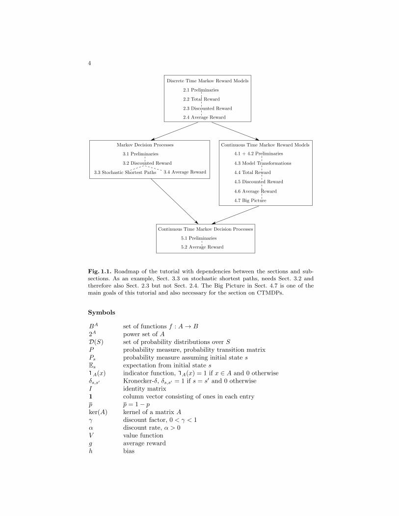
Fig. 1.1. Roadmap of the tutorial with dependencies between the sections and sub-sections. As an example, Sect. 3.3 on stochastic shortest paths, needs Sect. 3.2 andtherefore also Sect. 2.3 but not Sect. 2.4. The Big Picture in Sect. 4.7 is one of themain goals of this tutorial and also necessary for the section on CTMDPs.
Symbols
BA set of functions f : A→ B2A power set of AD(S) set of probability distributions over SP probability measure, probability transition matrixPs probability measure assuming initial state sEs expectation from initial state s1A(x) indicator function, 1A(x) = 1 if x ∈ A and 0 otherwiseδs,s′ Kronecker-δ, δs,s′ = 1 if s = s′ and 0 otherwiseI identity matrix1 column vector consisting of ones in each entryp p = 1− pker(A) kernel of a matrix Aγ discount factor, 0 < γ < 1α discount rate, α > 0V value functiong average rewardh bias
5
2 Discrete Time Markov Reward Models
2.1 Preliminaries
Definition 2.1. For a finite set S let D(S) :=δ : S → [0, 1] |
∑s∈S δ(s) = 1
be the space of discrete probability distributions over S.
Definition 2.2. A discrete-time Markov chain (DTMC) is a structureM = (S, P ) consisting of a finite set of states S (also called the state spaceof M) and a transition function P : S → D(S) which assigns to each state sthe probability P (s, s′) := (P (s)) (s′) to move to state s′ within one transition.A discrete-time Markov Reward Model (DTMRM) enhances a DTMC(S, P ) by a reward function R : S × S → R and is thus regarded as a structureM = (S, P,R).
In the definition, the rewards are defined over transitions, i.e. whenever a tran-sition from s to s′ takes place, a reward R(s, s′) is gained. Alternatively, aDTMRM can also be defined with state-based rewards R : S → R. There isa correspondence between transition-based and state-based reward models: Astate-based reward R(s) can be converted into a transition-based reward bydefining R(s, s′) := R(s) for all s′ ∈ S. On the other hand, a transition-basedreward R(s, s′) can be transformed by expectation into its state-based versionby defining R(s) :=
∑s′∈S R(s, s′)P (s, s′). Of course, this transformation can
not be inverted, but as we will see, the reward measures that we consider do notdiffer. Note that for state-based rewards there are two canonical but totally dif-ferent possibilities to define the point in time, when such a reward can be gained:either when a transition into the state or out of the state is performed. This cor-responds to the difference in the point of view for “arrivals” and “departures” ofjobs in queueing systems. When working with transition-based rewards R(s, s′)as in Definition 2.2, then such a confusion does not occur since R(s, s′) is gainedin state s after transition to s′ and thus its expected value R(s) corresponds tothe “departure” point of view. For our purposes we will mix both representionsand if we write R for a reward then it is assumed to be interpreted in a context-dependent way as either the state-based or the transition-based version.
Each bijective representation
ϕ : S → 1, 2, . . . , n , n := |S| (2.1)
of the state space as natural numbered indices allows to regard the rewards andthe transition probabilities as real-valued vectors in Rn respectively matrices inRn×n. We indirectly take such a representation ϕ, especially when we talk aboutP and R in vector notation. In this case the transition function P : S → D(S)can be regarded as a stochastic matrix, i.e. P1 = 1, where 1 = (1, . . . , 1)T isthe column vector consisting of all ones.
Example 2.1 (Queueing system). As a running example, consider a system con-sisting of a queue of capacity k and a service unit which can be idle, busy or
6
0,0,idle
0,1,busy
1,1,busy
0,0, vac
1,0,vac
1
2
3
4
5
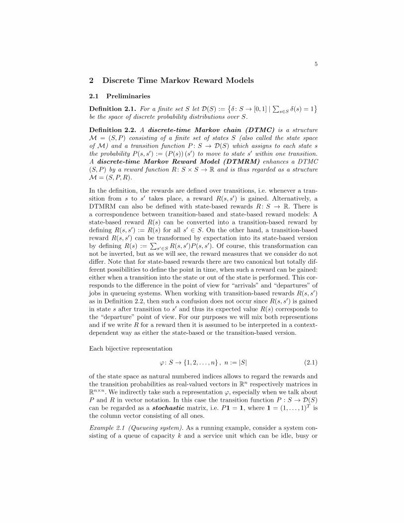
Fig. 2.1. Queueing model with queue capacity k = 1 and a service unit which can beidle, busy or on vacation. State (0, 1, busy) represents 0 jobs in the queue, 1 job inservice and server is busy. The dashed transitions represent the event that an incomingjob is discarded. The parameter values are q = 0.25, pd = 0.5, pv = 0.1 and pr = 0.25.Overlined probabilities are defined as p := 1− p.
on vacation (Fig. 2.1) [38]. A job arrives with probability q = 0.25 and gets en-queued if the queue is not full. If the server is idle and there is some job waitingin the queue, the server immediately gets busy and processes the job. At theend of each unit of service time, the server is done with the job with probabilitypd = 0.5 and can either go idle (and possibly getting the next job) or the serverneeds vacation with probability pv = 0.1. From the vacation mode the serverreturns with probability pr = 0.25. Figure 2.1 shows the model for the case ofqueue capacity k = 1, where transitions are split into regular transitions (solidlines) and transitions indicating that an incoming job gets discarded (dashedlines). The reward model is as follows: For each accomplished service a rewardof Racc = $100 is gained, regardless of whether the server moves to idle or to va-cation. However, the loss of a job during arrival causes a cost of Closs = −$1000.Therefore we consider the following state-based reward structures:
Rprofit =
00
Raccpd0
Raccpd
, Rcost =
000
ClossqprCloss (qpd + qpdpv)
, Rtotal = Rprofit +Rcost,
(2.2)where p := 1− p for some probability p. ut
There are several ways how the rewards gained for each taken transition (re-spectively for a visited state) can contribute to certain measures of interest. Intypical applications of performance evaluation, rewards are accumulated oversome time period or a kind of averaging over rewards is established. In orderto be able to define these reward measures formally, we need to provide somebasic knowledge on the stochastic state process induced by the DTMC part ofa DTMRM.
7
2.1.1 Sample SpaceFor a DTMC M = (S, P ) define Ω as the set of infinite paths, i.e.
Ω :=
(s0, s1, s2, . . . ) ∈ SN | P (si−1, si) > 0 for all i ≥ 1
(2.3)
and let B(Ω) be the Borel σ-algebra over Ω generated by the cylinder sets
C(s0, s1, . . . , sN ) := ω ∈ Ω | ωi = si ∀i ≤ N .
Each s ∈ S induces a probability space (Ω,B(Ω), Ps) with a probability distri-bution Ps : B(Ω)→ R over paths, such that for each cylinder set C(s0, . . . , sN ) ∈B(Ω)
Ps (C(s0, . . . , sN )) = δs0,sP (s0, s1)P (s1, s2) . . . P (sN−1, sN ),
where δ is the Kronecker-δ, i.e. δs,s′ = 1 if s = s′ and 0 otherwise.
Definition 2.3. The DTMC M induces the stochastic state process (Xn)n∈Nover Ω which is a sequence of S-valued random variables such that Xn(ω) := snfor ω = (s0, s1, . . . ) ∈ Ω.
Note that
Ps(Xn = s′) =∑
s1,...,sn−1
P (s, s1)P (s1, s2) . . . P (sn−2, sn−1)P (sn−1, s′) = Pn(s, s′),
where∑s1,...,sn−1
denotes summation over all tuples (s1, . . . , sn−1) ∈ Sn−1. The
process Xn also fulfills the Markov property (or memorylessness): For alls, s′, s0, s1, . . . sn−1 ∈ S it holds that
Ps0(Xn+1 = s′ | X1 = s1, . . . , Xn−1 = sn−1, Xn = s) = P (s, s′), (2.4)
i.e. if the process is in state s at the current point in time n, then the probabilityto be in state s′ after the next transition does not depend on the history ofthe process consisting of the initial state X0 = s0 and the traversed statesX1 = s1, . . . , Xn−1 = sn−1 up to time n− 1.We denote the expectation operator over (Ω,B(Ω), Ps) as Es. For a functionf : Sn+1 → R it holds
Es [f(X0, X1, . . . , Xn)] =∑
s1,...,sn
f(s, s1 . . . , sn)P (s, s1)P (s1, s2) . . . P (sn−1, sn).
In vector representation we often write E [Y ] := (Es [Y ])s∈S for the vector con-sisting of expectations of a real-valued random variable Y .
2.1.2 State ClassificationIn the following, we briefly outline the usual taxonomy regarding the classifica-tion of states for a discrete-time Markov chain M = (S, P ). The state processXn induced byM allows to classify the states S with respect to their recurrence

8
and reachability behavior. If X0 = s is the initial state then the random vari-able Ms := inf n ≥ 1 | Xn = s ∈ N ∪ ∞ is the first point in time when theprocess Xn returns to s. If along a path ω ∈ Ω the process never returns to sthen Ms(ω) = inf ∅ = ∞. If there is a positive probability to never come backto s, i.e. Ps(Ms = ∞) > 0 then the state s is called transient. Otherwise, ifPs(Ms <∞) = 1 then s is recurrent. We denote St as the set of transient statesand Sr as the set of recurrent states. A state s′ is reachable from s (denoted bys → s′), if there exists n ∈ N with Ps(Xn = s′) > 0. The notion of reachabilityinduces the (communcation) equivalence relation
s↔ s′ ⇔ s→ s′ and s′ → s.
This relation further partitions the set of recurrent states Sr into the equivalenceclasses Sri , i = 1, . . . , k such that the whole state space S can be written as the
disjoint union S =⋃ki=1 S
ri ∪ St. Each of these equivalence classes Sri is called a
closed recurrent class, since (by the communication relation) for every s ∈ Srithere are no transitions out of this class, i.e. P (s, s′) = 0 for all s′ ∈ S\Sri . For thisreason each Sri is a minimal closed subset of S, i.e. there is no proper nonemptysubset of Sri which is closed. In case a closed recurrent class consists only of onestate s, then s is called absorbing. The DTMCM is unichain if there is onlyone recurrent class (k = 1) and if in addition St = ∅ then M is irreducible. ADTMC that is not unichain will be called multichain. The queueing system inExample 2.1 is irreducible, since every state is reachable from every other state.For discrete-time Markov chains there are some peculiarities regarding the long-run behavior of the Markov chain as n → ∞. If X0 = s is the initial stateand the limit ρs(s
′) := limn→∞ Ps(Xn = s′) exists for all s′, then ρs ∈ D(S)is called the limiting distribution from s. In general this limit does not needto exist, since the sequence Ps(Xn = s′) = Pn(s, s′) might have oscillationsbetween distinct accumulation points. This fact is related to the periodicity of astate: From state s the points in time of possible returns to s are given by theset Rs := n ≥ 1 | Ps(Xn = s) > 0. If all n ∈ Rs are multiples of some naturalnumber d ≥ 2 (i.e. Rs ⊆ kd | k ∈ N) then the state s is called periodic and theperiodicity of s is the largest such integer d. Otherwise s is called aperiodicand the periodicity of s is set to 1. The periodicity is a class property and meansthat for every closed recurrent class Sri and for all s, s′ ∈ Sri the periodicity of sand s′ is the same. A Markov chain which is irreducible and aperiodic is oftencalled ergodic in the literature. As an example, a two-state Markov chain withtransition probability matrix
P =
(0 11 0
)is irreducible but not ergodic, since it is periodic with periodicity 2.One can show that a recurrent state s in a DTMC with finite state space is ape-riodic if and only if for all s′ ∈ S the sequence Pn(s, s′) converges. Therefore,the limiting distribution ρs exists (for s recurrent) if and only if s is aperiodic.In this case ρs(s
′) =∑t ρs(t)P (t, s′) for all s′, which is written in vector no-
tation by ρs = ρsP . This equation is often interpreted as the invariance (or
9
stationarity) condition: If ρs(s′) is the probability to find the system in state s′
at some point in time, then this probability remains unchanged after the systemperforms a transition. In general, there can be several distributions ρ ∈ D(S)with the invariance property ρ = ρP and any such distribution ρ is called astationary distribution. It holds that the set of all stationary distributionsforms a simplex in RS and the number of vertices of this simplex is exactlythe number of recurrent classes k. Therefore, in a unichain model M there isonly one stationary distribution ρ and if M is irreducible then ρ(s) > 0 for alls ∈ S. Since a limiting distribution is stationary it further holds that if M isunichain and aperiodic (or even ergodic), then for all initial states s the limitingdistribution ρs exists and ρs = ρ is the unique stationary distribution and thusindependent of s.We will draw on the stationary distributions (and also the periodic behavior) ofa Markov chain in Sect. 2.4, where we will outline the average reward analysis.In order to make the intuition on the average reward clear, we will also workwith the splitting S =
⋃ki=1 S
ri ∪ St into closed recurrent classes and transient
states. The computation of this splitting can be performed by the Fox-Landistate classification algorithm [15]. It finds a representation ϕ of S (see (2.1))such that P can be written as
P =
P1 0 0 . . . 0 00 P2 0 . . . 0 0...
......
. . .... 0
0 0 0 . . . Pk 0
P1 P2 P3 . . . Pk Pk+1
(2.5)
where Pi ∈ Rri×ri , Pi ∈ Rt×ri , Pk+1 ∈ Rt×t with ri := |Sri | for i = 1, . . . , k andt := |St|. The matrix Pi represents the transition probabilities within the i-th
recurrent class Sri and Pi the transition probabilities from transient states St
into Sri if i = 1, . . . , k, respectively transitions within St for i = k + 1. Everyclosed recurrent class Sri can be seen as a DTMC Mi = (Sri , Pi) by omittingincoming transitions from transient states. It holds that Mi is irreducible andthus has a unique stationary distribution ρi ∈ D(Sri) with ρi(s) > 0 for alls ∈ Sri . This distribution ρi can be extended to a distribution ρi ∈ D(S) onS by setting ρi(s) := 0 for all s ∈ S \ Sri . Note that ρi is also stationary onM. Since transient states St of M are left forever with probability 1 (into therecurrent classes), every stationary distribution ρ ∈ D(S) fulfills that ρ(s) = 0for all s ∈ St. Thus, an arbitrary stationary distribution ρ ∈ D(S) is a convex
combination of all the ρi, i.e. ρ(s) =∑ki=1 aiρi(s) with ai ≥ 0 and
∑ki=1 ai = 1.
(This forms the k-dimensional simplex with vertices ρi as mentioned above.)
2.1.3 Reward MeasureWe now consider a DTMRM M = (S, P,R) and want to describe in the fol-lowing sections several ways to accumulate the rewards R(s, s′) along pathsω = (s0, s1, . . . ) ∈ Ω. As an example, for a fixed N ∈ N ∪ ∞ (also called the
10
horizon length) we can accumulate the rewards for the first N transitions bysimple summation: the reward gained for the i-th transition is R(si−1, si) and is
summed up to∑Ni=1R(si−1, si), which is regarded as the value of the path ω for
the first N transitions. The following definition introduces the notion of a valuefor state-based models, with which we will be concerned in this tutorial.
Definition 2.4. Consider a state-based model M with state space S and a realvector space V. A reward measure R is an evaluation of the model M thatmaps M with an optional set of parameters to the value V ∈ V of the model.If V is a vector space of functions over S, i.e. V = RS = V : S → R, then avalue V ∈ V is also called a value function of the model.
Note that we consider in this definition an arbitrary state-based model, whichcan have discrete time (e.g. DTMRM or MDP, cf. Sect. 3) or continuous time(CTMRM or CTMDP, cf. Sects. 4 and 5). We will mainly consider vector spacesV which consist of real-valued functions. Beside value functions V ∈ RS whichmap every state s ∈ S to a real value V (s) ∈ R, we will also consider valuefunctions that are time-dependent. For example, if T denotes a set of time valuesthen V = RS×T consists of value functions V : S × T → R such that V (s, t) ∈ Ris the real value of state s ∈ S at the point in time t ∈ T . In typical applicationsT is a discrete set for discrete-time models (e.g. T = N or T = 0, 1, . . . , N), orT is an interval for continuous-time models (e.g. T = [0,∞) or T = [0, Tmax]).The difference between the notion of a reward measure R and its value functionV is that a reward measure can be seen as a measure type which needs additionalparameters in order to be able to formally define its value function V . Examplesfor such parameters are the horizon length N , a discount factor γ (in Sect. 2.3)or a discount rate α (in Sect. 4.5). If clear from the context, we use the notionsreward measure and value (function) interchangeably.
2.2 Total Reward Measure
We now define the finite-horizon and infinite-horizon total reward measureswhich formalize the accumulation procedure along paths by summation as men-tioned in the motivation of Definition 2.4. The finite-horizon reward measure isused as a basis upon which all the following reward measures will be defined.
Definition 2.5. LetM be a DTMRM with state process (Xn)n∈N and N <∞ afixed finite horizon length. We define the finite-horizon total value functionVN : S → R by
VN (s) := Es
[N∑i=1
R(Xi−1, Xi)
]. (2.6)
If for all states s the sequence Es[∑N
i=1 |R(Xi−1, Xi)|]
converges with N →∞,
we define the (infinite-horizon) total value function as
V∞(s) := limN→∞
VN (s).
11
In general VN (s) does not need to converge as N → ∞. For example, if allrewards for every recurrent state are strictly positive, then accumulation of pos-itive values diverges to ∞. Even worse, if the rewards have different signs thentheir accumulation can also oscillate. In order not to be concerned with suchoscillations, we impose as a stronger condition the absolute convergence for theinfinite-horizon case as in the definition.
As next we want to provide a method which helps to evaluate the total rewardmeasure for the finite and infinite horizon cases. The proof of the followingtheorem can be found in the Appendix (page 81).
Theorem 2.1 (Evaluation of the Total Reward Measure).
(i) The finite-horizon total value VN (s) can be computed iteratively through
VN (s) = R(s) +∑s′∈S
P (s, s′)VN−1(s′),
where V0(s) := 0 for all s ∈ S.
(ii) If the infinite-horizon total value V∞(s) exists, then it solves the system oflinear equations
V∞(s) = R(s) +∑s′∈S
P (s, s′)V∞(s′). (2.7)
We formulate the evaluation of the total value function in vector notation:
VN = R+ PVN−1 =
N∑i=1
P i−1R. (2.8)
For the infinite-horizon total value function it holds
V∞ = R+ PV∞ respectively (I − P )V∞ = R. (2.9)
Note that Theorem 2.1 states that if V∞ exists, then it solves (2.9). On theother hand the system of equations (I−P )X = R with the variable X may haveseveral solutions, since P is stochastic and thus the rank of I−P is not full. Thenext proposition shows a necessary and sufficient condition for the existence ofV∞ in terms of the reward function R. Furthermore, it follows that if V∞ existsthen V∞(s) = 0 on all recurrent states s and V∞ is also the unique solution to(I − P )X = R with the property that X(s) = 0 for all recurrent states s. Aproof (for aperiodic Markov chains) can be found in the Appendix on page 81.
Proposition 2.1. For a DTMRM (S, P,R) let S =⋃ki=1 S
ri ∪ St be the par-
titioning of S into k closed recurrent classes Sri and transient states St. Theinfinite-horizon total value function V∞ exists if and only if for all i = 1, . . . , kand for all s, s′ ∈ Sri it holds that
R(s, s′) = 0.
12
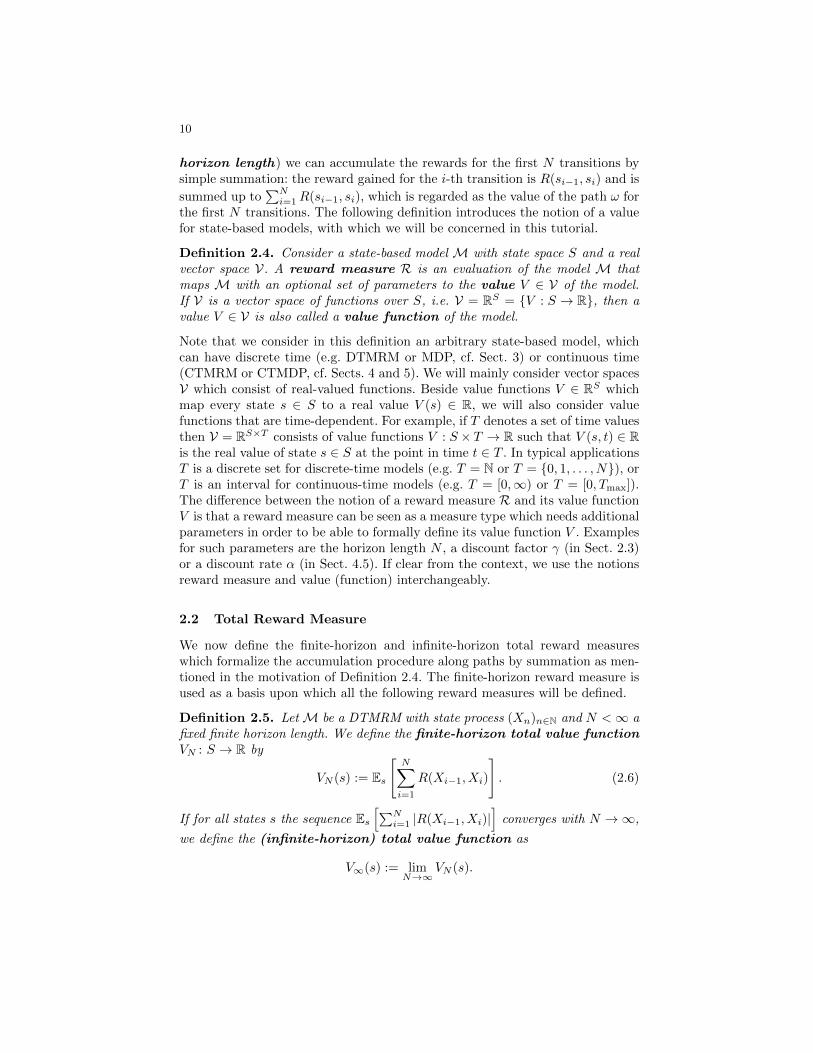
Example 2.2. Let us go back to the queueing model introduced in Example 2.1.The finite-horizon total value function for the first 30 transitions and rewardfunction R := Rtotal is shown in Fig. 2.2 for the initial state sinit = (0, 0, idle).
5 10 15 20 25 30N
-40
-20
20
40
VN
Fig. 2.2. Finite-horizon total value function with horizon length N = 30 for the queue-ing model in Example 2.1 and initial state sinit = (0, 0, idle).
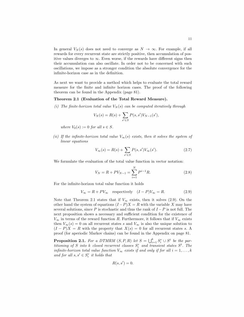
As one can see, at the beginning the jobs need some time to fill the system(i.e. both the queue and the server) and thus the expected accumulated rewardincreases. But after some time steps the high penalty of Closs = −$1000 fordiscarding a job outweighs the accumulation of the relatively small rewardRacc =$100 for accomplishing a job and the total value decreases. The infinite-horizontotal value does not exist in this model, since VN (sinit) diverges to −∞. However,in case the total reward up to the first loss of a job is of interest, one canintroduce an auxiliary absorbing state loss with reward 0, which represents thatan incoming job has been discarded (Fig. 2.3).
0,0idle
0,1busy
1,1busy
0,0vac
1,0vac
loss
1 3 5
2 4 6
Fig. 2.3. Queueing model enhanced with an auxiliary absorbing state ’loss’ represent-ing the loss of an incoming job due to a full queue.
Since the single recurrent state loss in this DTMRM has reward 0, the total valuefunction exists and fulfills (2.7) (respectively (2.9)) with R(s) := Rprofit(s) for

13
s 6= loss (see (2.2)) and R(loss) := 0. Note that I −P has rank 5 since P definesan absorbing state. From R(loss) = 0 it follows that the total value function V∞is the unique solution for (2.7) with the constraint V∞(loss) = 0 and is given by
V∞ ≈ (1221.95, 980.892, 1221.95, 659.481, 950.514, 0)T. ut
2.3 Horizon-expected and Discounted Reward Measure
In order to be able to evaluate and compare the performance of systems in whichthe total value does not exist, we need other appropriate reward measures. Inthis and the following subsection, we will present two other typically used rewardmeasures: the discounted and the average reward measure. Roughly speaking,the average reward measures the derivation of the total value with respect to thehorizon length N , i.e. its average growth. The discounted measure can be usedif the horizon length for the system is finite but a priori unknown and can beassumed as being random (and memoryless). In order to define the discountedreward measure, we first introduce the more general horizon-expected rewardmeasure.
Definition 2.6. Let M = (S, P,R) be a DTMRM and consider a random hori-zon length N for M, i.e. N is a random variable over N that is independent ofthe state process Xn ofM. Let V(N) denote the random finite-horizon total value
function that takes values inVn ∈ RS | n ∈ N
. Define the horizon-expected
value function by
V (s) := E[V(N)(s)
],
if the expectation exists for all s ∈ S, i.e. |V(N)(s)| has finite expectation.
In order to be formally correct, the random variable V(N)(s) is the conditional ex-
pectation V(N)(s) = Es[∑N
i=1R(Xi−1, Xi) | N]
and thus if N = n then V(N)(s)
takes the value Es[∑N
i=1R(Xi−1, Xi) | N = n]
=Es [∑ni=1R(Xi−1, Xi)] = Vn(s).
By the law of total expectation it follows that
V (s) = E
[Es
[N∑i=1
R(Xi−1, Xi) | N
]]= Es
[N∑i=1
R(Xi−1, Xi)
],
i.e. V (s) is a joint expectation with respect to the product of the probabilitymeasures of N and all the Xi.
The following lemma presents a natural sufficient condition that ensures theexistence of the horizon-expected value function.
Lemma 2.1. If the random horizon length N has finite expectation E [N ] <∞then V (s) exists.
14
Proof. Since the state space is finite there exists C ∈ R such that |R(s, s′)| ≤ C∀s, s′ ∈ S. Therefore
|Vn(s)| ≤ Es
[n∑i=1
|R(Xi−1, Xi)|
]≤ n · C
and thus
E[|V(N)(s)|
]=
∞∑n=0
|Vn(s)| · P (N = n) ≤ C · E [N ] <∞. ut
In many applications the horizon length is considered to be memoryless, i.e.P (N > n+m | N > m) = P (N > n) and is therefore geometrically distributed.This fact motivates the following definition.
Definition 2.7. For γ ∈ (0, 1) let N be geometrically distributed with parameter1 − γ, i.e. P (N = n) = γn−1(1 − γ) for n = 1, 2, . . . . In this case the horizon-expected value function is called discounted value function with discountfactor γ (or just γ-discounted value function) and is denoted by V γ .
As for the total value function in Sect. 2.2 we can explicitly compute the dis-counted value function:
Theorem 2.2 (Evaluation of the Discounted Reward Measure). For adiscount factor γ ∈ (0, 1) it holds that
V γ(s) = limn→∞
Es
[n∑i=1
γi−1R(Xi−1, Xi)
]. (2.10)
Furthermore, V γ is the unique solution to the system of linear equations
V γ(s) = R(s) + γ∑s′∈S
P (s, s′)V γ(s′) (2.11)
which is written in vector notation as
(I − γP )V γ = R.
Proof. Let N be geometrically distributed with parameter γ. By conditionalexpectation we get
V γ(s) = E
[Es
[N∑i=1
R(Xi−1, Xi) | N
]]=
∞∑n=1
Es
[n∑i=1
R(Xi−1, Xi)
]P (N = n)
= (1− γ)
∞∑i=1
Es [R(Xi−1, Xi)]
∞∑n=i
γn−1 =
∞∑i=1
Es [R(Xi−1, Xi)] γi−1,
which gives (2.10). The derivation of the linear equations (2.11) is completelyanalogous to the total case by comparing (2.10) to (2.6) (see proof of Theorem2.1). Since I − γP has full rank for γ ∈ (0, 1) the solution is unique. ut

15
Equation (2.10) yields also another characterization of the discounted rewardmeasure. Along a path ω = (s0, s1, s2, . . . ) the accumulated discounted rewardis R(s0, s1) + γR(s1, s2) + γ2R(s2, s3) + . . . . The future rewards R(si, si+1) arereduced by the factor γi < 1 in order to express some kind of uncertainty aboutthe future reward value (e.g. induced by inflation). In many applications, thediscounted reward measure is used with a high discount factor close to 1 whichstill avoids possible divergence of the infinite-horizon total value. Qualitativelyspeaking, for high γ < 1 the sequence γi decreases for the first few points in timei slowly, but exponentially to 0. If we assume that the rewards R(s) are close toeach other for each state s, then the rewards accumulated within the first fewtime steps approximately give the discounted value.
Remark 2.1. Note that the discounted value function can be equivalently char-acterized as an infinite-horizon total value function by adding an absorbing andreward-free final state abs to the state space S such that abs is reachable fromany other state with probability 1 − γ and any other transition probability ismultiplied with γ (see Fig. 2.4). Since abs is eventually reached on every pathwithin a finite number of transitions with probability 1 and has reward 0, itcharacterizes the end of the accumulation procedure. The extended transitionprobability matrix P ′ ∈ R(|S|+1)×(|S|+1) and the reward vector R′ ∈ R|S|+1 aregiven by
P ′ =
(γP (1− γ)10 1
)and R′ =
(R0
),
where 1 = (1, . . . , 1)T . Since abs is the single recurrent state and R(abs) = 0 itfollows by Proposition 2.1 that V∞ exists. Furthermore, it satisfies (I−P ′)V∞ =R′ and because V∞(abs) = 0 it is also the unique solution with this property.
On the other hand (V γ , 0)T
is also a solution and thus V∞ = (V γ , 0)T
.
s''s'
s
abss''s'
s
Fig. 2.4. Equivalent characterization of the γ-discounted reward measure as a totalreward measure by extending the state space with an absorbing reward-free state.
Example 2.3. As an example we analyze the queueing model from Example 2.1with respect to the discounted reward measure. Figure 2.5 shows V γ(s) for theinital state sinit = (0, 0, idle) as a function of γ. As we see, for small valuesof γ the discounted values are positive, since the expected horizon length 1
1−γis also small and thus incoming jobs have a chance to be processed and notdiscarded within that time. However for γ approaching 1, the expected horizonlength gets larger and the accumulation of the negative reward Closs = −$1000for discarding jobs in a full queue prevails. ut

16
0.6 0.7 0.8 0.9 1.0g
-400
-300
-200
-100
V g
Fig. 2.5. Discounted reward V γ(sinit) as a function of γ for the queueing model inExample 2.1 and initial state sinit = (0, 0, idle).
2.4 Average Reward Measure
We now provide another important reward measure for the case that the horizonlength is infinite (and not random as assumed in Sect. 2.3). We assume for thissection that the reader is familiar with the concept of periodicity as presentedin Sect. 2.1.2. If for a DTMRM M = (S, P,R) the infinite-horizon total valuefunction V∞ does not exist, then either VN (s) diverges to ±∞ for some state sor VN (s) is oscillating over time. The problem with this measure is that V∞ in-finitely often collects the rewards and sums them all up. Instead of building sucha total accumulation, one can also measure the system by considering the gainedrewards only per time step. As an example, consider an ergodic modelM in thelong run with limiting distribution ρ := ρs given by ρs(s
′) := limn→∞ Pn(s, s′)for an arbitrary intial state s. Then in steady-state the system is rewarded ateach time step with ρR =
∑s ρ(s)R(s) ∈ R, i.e. an average of all the rewards
R(s) weighted by the probability ρ(s) that the system occupies state s in steady-state. But averaging the rewards R(s) shall not be restricted to only those modelsM for which a limiting distribution exists. First of all, the limiting distributionρs can depend on the initial state s, if M has several closed recurrent classes.More important, the limiting distribution might even not exist, as one can seefor the periodic model with
P =
(0 11 0
)and R =
(24
).
However, in this case one would also expect an average reward of 3 for each timestep and for every state, since P is irreducible and has the unique stationarydistribution ρ = (0.5, 0.5). This means that the average reward measure shallalso be applicable to models for which the limiting distribution does not exist.Instead of computing an average per time step in steady-state, one can alsothink of calculating an average in the long-run by accumulating for each horizonlength N the total value VN and dividing it by the time N . The limit of the
17
sequence of these finite horizon averages establishes the desired long-run aver-age. As we will see in Proposition 2.2, this long-run average always converges,independent of the structure of the underyling DTMRM. Furthermore, in casethe limiting distribution exists then the steady-state average and the long-runaverage coincide and thus the long-run average fulfills the desired requirementsfrom the motivation.
Definition 2.8. The average reward measure (or gain) of a DTMRM withvalue function g(s) is defined by
g(s) := limN→∞
1
NVN (s)
if the limit exists.
In the following, we summarize well-known results from linear algebra whichfirst of all directly imply that the average reward exists (at least for finite statespaces) and furthermore also allow us to provide methods for its evaluation.
Definition 2.9. For a stochastic matrix P define the limiting matrices P∞
and P ∗ as:
P∞ := limN→∞
PN and P ∗ := limN→∞
1
N
N∑i=1
P i−1,
if the limits exist. (P ∗ is the Cesaro limit of the sequence P i.)
Suppose that P ∗ exists. Then the average reward can be computed by
g = P ∗R, (2.12)
since by (2.8) it holds that
g(s) = limN→∞
1
NVN (s) = lim
N→∞
1
N
N∑i=1
(P i−1R
)(s) = (P ∗R) (s).
Note also that if P∞ exists, then the i-th row in P∞ (with i = ϕ(s), see (2.1))represents the limiting distribution ρi of the model, given that the initial state ofthe system is s. By the motivation from above it should also hold that g(s) = ρiR.The following proposition relates these two quantities to each other. We referfor proof to [33].
Proposition 2.2. Consider a DTMC M = (S, P ) with finite state space.
(i) The limiting matrix P ∗ exists.(ii) If P∞ exists, then P ∗ = P∞.
(iii) If P is aperiodic then P∞ exists and if in addition P is unichain (or ergodic)with limiting distribution ρ then ρP = ρ and P∞ has identical rows ρ, i.e.
P ∗ = P∞ = 1ρ,
where 1 = (1, . . . , 1)T is the column vector consisting of all ones.
18
From Proposition 2.2(ii) it follows that the definition of the average reward cor-responds to its motivation from above in the case that the limiting distributionρi exists for all i. However, in the case of periodic DTMRMs (when the limitingdistribution is not available), Proposition 2.2(i) ensures that at least P ∗ existsand due to (2.12) this is sufficient for the computation of the average reward.
Remark 2.2. The limiting matrix P ∗ satisfies the equalities
PP ∗ = P ∗P = P ∗P ∗ = P ∗. (2.13)
P ∗ can be computed by partitioning the state space S = ∪ki=1Sri ∪St into closed
recurrent classes Sri and transient states St which results in a representation of Pas in (2.5). Let the row vector ρi ∈ Rri denote the unique stationary distributionof Pi, i.e. ρiPi = ρi. Then
P ∗ =
P ∗1 0 0 . . . 0 00 P ∗2 0 . . . 0 0...
......
. . .... 0
0 0 0 . . . P ∗k 0
P ∗1 P ∗2 P ∗3 . . . P ∗k 0
(2.14)
where P ∗i = 1ρi has identical rows ρi ∈ Rri and P ∗i = (I − Pk+1)−1PiP∗i
consists of trapping probabilities from transient states into the i-th recurrentclass. It follows that the average reward g is constant on each recurrent class,i.e. g(s) = gi := ρiRi for all s ∈ Sri where Ri ∈ Rri is the vector of rewards onSri . On transient states the average reward g is a weighted sum of all the gi withweights given by the trapping probabilities.
We want to provide another method to evaluate the average reward measure,because it will be useful for the section on MDPs. This method relies on the keyaspect of a Laurent series decomposition which also links together the three pro-posed measures total reward, discounted reward and average reward. Considerthe discounted value V γ = (I − γP )−1R as a function of γ (cf. Theorem 2.2). Ifthe total value function V∞ = (I − P )−1R exists then V γ converges to V∞ asγ 1. But what happens if V∞ diverges to ∞ or −∞? In this case V γ has apole singularity at γ = 1 and can be expanded into a Laurent series. Roughlyspeaking, a Laurent series generalizes the concept of a power series for (differ-entiable) functions f with poles, i.e. points c at the boundary of the domain off with limx→c f(x) = ±∞. In such a case, f can be expanded in some neigh-borhood of c into a function of the form
∑∞n=−N an(x − c)n for some N ∈ N
and an ∈ R, which is a sum of a rational function and a power series. In ourcase, since γ 7→ V γ might have a pole at γ = 1, the Laurent series is of the formV γ =
∑∞n=−N an(γ − 1)n for γ close to 1. The coefficients an in this expansion
are given in Theorem 2.3 in the sequel which can be deduced from the followingLemma. A proof for the lemma can be found in [33].
Lemma 2.2 (Laurent Series Expansion). For a stochastic matrix P thematrix (I − P + P ∗) is invertible. Let
H := (I − P + P ∗)−1 − P ∗.
19
There exists δ > 0 such that for all 0 < ρ < δ the Laurent series of the matrix-valued function ρ 7→ (ρI + (I − P ))−1 is given by
(ρI + (I − P ))−1 = ρ−1P ∗ +
∞∑n=0
(−ρ)nHn+1.
Theorem 2.3 (Laurent Series of the Discounted Value Function). LetM = (S, P,R) be a DTMRM. For a discount factor γ < 1 close to 1 writeγ(ρ) := 1
1+ρ where ρ = 1−γγ > 0 and consider the discounted value V γ(ρ) as a
function of ρ.
(i) The Laurent series of ρ 7→ V γ(ρ) at 0 is given (for small ρ > 0) by
V γ(ρ) = (1 + ρ)
(ρ−1g +
∞∑n=0
(−ρ)nHn+1R
), (2.15)
where g is the average reward.(ii) It holds that
V γ =1
1− γg + h+ f(γ) (2.16)
where h := HR and f is some function with limγ1
f(γ) = 0. Furthermore,
g = limγ1
(1− γ)V γ .
Proof. (i) We apply the Laurent series from Lemma 2.2 as follows:
V γ = (I − γP )−1R = (1 + ρ)(ρI + (I − P ))−1R
= (1 + ρ)
(ρ−1P ∗R+
∞∑n=0
(−ρ)nHn+1R
)
and the claim follows from (2.12). Furthermore, by substituting γ = (1 + ρ)−1
V γ =1
γ
(γ
1− γg + h+
∞∑n=1
(γ − 1
γ
)nHn+1R
)=
1
1− γg + h+ f(γ)
where f(γ) :=1− γγ
h+
∞∑n=1
(γ − 1
γ
)nHn+1R and f(γ)→ 0 when γ 1 such
that (ii) follows. ut
The vector h in (2.16) is called the bias for the DTMRM. We provide an equiva-lent characterization for h that allows a simpler interpretation of the term “bias”as some sort of deviation. If the reward function R is replaced by the averagereward g, such that in every state s the average reward g(s) is gained instead of
R(s), then the finite horizon total reward is given by GN (s) := Es[∑N
i=1 g(Xi)],

20
where Xi is the state process. In this case ∆N := VN − GN describes the de-viation in accumulation between the specified reward R and its correspondingaverage reward g = P ∗R within N steps. By (2.8) it holds that
∆N =
N−1∑n=0
Pn(R− g) =
N−1∑n=0
(Pn − P ∗)R.
Note that Pn − P ∗ = (P − P ∗)n for all n ≥ 1 which follows from (2.13) and∑nk=0(−1)k
(nk
)= 0 applied on (P−P ∗)n =
∑nk=0
(nk
)Pn−k(−P ∗)k. If we assume
that ∆N converges for any reward function R then∑∞n=0(P − P ∗)n converges
and it holds that∑∞n=0(P − P ∗)n = (I − (P − P ∗))−1. It follows
limN→∞
∆N =∞∑n=0
(Pn − P ∗)R =
((I − P ∗) +
∞∑n=1
(P − P ∗)n)R =( ∞∑
n=0
(P − P ∗)n − P ∗)R =
((I − (P − P ∗))−1 − P ∗
)R = HR = h.
Therefore, the bias h(s) is exactly the long-term deviation between VN (s) andGN (s) as N →∞. This means that the value h(s) is the excess in the accumu-lation of rewards beginning in state s until the system reaches its steady-state.Remember that g is constant on recurrent classes. Thus, for a recurrent state s
it holds that GN (s) = Es[∑N
i=1 g(Xi)]
= g(s)N is linear in N and g(s)N +h(s)
is a linear asymptote for VN (s) as N →∞, i.e. VN (s)− (g(s)N +h(s))→ 0 (seeFig. 2.6). The matrix H is often called the deviation matrix for the DTMRMsince it maps any reward function R to the corresponding long-term deviationrepresented by the bias h = HR.
5 10 15 20N
- 5
5
10
15
20
Fig. 2.6. Interpretation of the bias h(s) as the limit of the deviation VN (s) − GN (s)as N →∞. For a recurrent state s it holds that GN (s) = g(s)N .
Another characterization for the bias can be given by considering ∆N as afinite-horizon total value function for the average-corrected rewards R − g, i.e.

21
∆N (s) = Es[∑N
i=1 (R(Xi)− g(Xi))]. For this reason the bias h is a kind of
infinite-horizon total value function for the model (S, P,R− g) 1.In the above considerations we have assumed that ∆N converges (for any re-ward function R), which is guaranteed if the DTMRM is aperiodic [33]. On theother hand, one can also construct simple periodic DTMRMs for which ∆N isoscillating. For this reason, there is a similar interpretation of the bias h if theperiodicity of P is averaged out (by the Cesaro limit). This is related to thedistinction between the two limiting matrices P∞ and P ∗ from Definition 2.9and goes beyond the scope of this tutorial. In Sect. 4 we will introduce the av-erage reward for continuous-time models (where periodicity is not a problem)and define the deviation matrix H by a continuous-time analogon of the discreterepresentation H =
∑∞n=0(Pn − P ∗).
Remark 2.3. In the Laurent series expansion of V γ respectively V γ(ρ) as in (2.15)the vector value Hn+1R for n ≥ 0 is often called the n-bias of V γ and thereforethe bias h = HR is also called the 0-bias. We will see in Sect. 3.4 (and especiallyRemark 3.6) that these values play an important role in the optimization ofMDPs with respect to the average reward and the n-bias measures.
We now provide some methods for computing the average reward based on thebias h of a DTMRMM = (S, P,R). IfM is ergodic then from Proposition 2.2 itholds that P ∗ = 1ρ and thus the average reward g = P ∗R = 1(ρR) is constantlyρR for each state. In the general case (e.g. M is multichain or periodic), thefollowing theorem shows how the bias h can be involved into the computationof g. The proof is based on the following equations that reveal some furtherconnections between P ∗ and H:
P ∗ = I − (I − P )H and HP ∗ = P ∗H = 0. (2.17)
These equations can be deduced from the defining equation for H in Lemma 2.2together with (2.13).
Theorem 2.4 (Evaluation of the Average Reward Measure). The aver-age reward g and the bias h satisfy the following system of linear equations:(
I − P 0I I − P
)(gh
)=
(0R
). (2.18)
Furthermore, a solution (u, v) to this equation implies that u = P ∗R = g is theaverage reward and v differs from the bias h up to some w ∈ ker(I − P ), i.e.v − w = h.
1 Note that in Definition 2.5 we restricted the existence of the infinite-horizon totalvalue function to an absolute convergence of the finite-horizon total value function∆N . By Proposition 2.1 this is equivalent to the fact that the rewards are zero onrecurrent states. For the average-corrected model this restriction is in general notsatisfied. The reward function R − g can take both positive and negative values onrecurrent states which are balanced out by the average reward g such that ∆N isconverging (at least as a Cesaro limit).
22
Proof. We first show that g and h are solutions to (2.18). From PP ∗ = P ∗ itfollows that Pg = PP ∗R = P ∗R = g and from (2.17) we have
(I − P )h = (I − P )HR = (I − P ∗)R = R− g
and thus (g, h) is a solution to (2.18). Now for an arbitrary solution (u, v) to(2.18) it follows that
(I−P+P ∗)u=(I−P )u+P ∗u+P ∗(I−P )v=(I−P )u+P ∗(u+(I−P )v) = 0+P ∗R.
Since I − P + P ∗ is invertible by Lemma 2.2, we have
u = (I − P + P ∗)−1P ∗R =((I − P + P ∗)−1 − P ∗ + P ∗
)P ∗R = HP ∗R+ P ∗R.
From (2.17) it holds that HP ∗ = 0 and thus u = P ∗R = g. Furthermore, sinceboth h and v fulfill (2.18) it follows that
(I − P )v = R− g = (I − P )h
and thus w := v − h ∈ ker(I − P ), such that h = v − w. ut
From (2.18) it holds that h = (R− g) +Ph, which reflects the motivation of thebias h as a total value function for the average-corrected model (S, P,R − g).Furthermore, the theorem shows that the equation h = (R − u) + Ph is onlysolvable for u = g. This means that there is only one choice for u in order tobalance out the rewards R such that the finite-horizon total value function ∆N
for the model (S, P,R− u) converges (as a Cesaro limit).
Remark 2.4. Assume that S =⋃ki=1 S
ri ∪St is the splitting of the state space of
M into closed recurrent classes Sri and transient states St.
(i) As we saw from (2.12) and (2.14) one can directly compute g from the split-ting of S. Equation (2.18) shows that such a splitting is not really necessary.However, performing such a splitting (e.g. by the Fox-Landi algorithm [15])for the computation of g by P ∗R can be more efficient than simply solving(2.18) [33].
(ii) In order to compute g from (2.18) it is enough to compute the bias h up toker(I − P ). The dimension of ker(I − P ) is exactly the number k of closedrecurrent classes Sri . Hence, if the splitting of S is known, then v(s) can beset to 0 for some arbitrary chosen state s in each recurrent class Sri (leadingto a reduction in the number of equations in Theorem 2.4).
(iii) In order to determine the bias h, it is possible to extend (2.18) toI − P 0 0I I − P 00 I I − P
uvw
=
0R0
. (2.19)
It holds that if (u, v, w) is a solution to (2.19) then u = g and v = h [33].In a similar manner, one can also establish a system of linear equations inorder to compute the n-bias values (see Remark 2.3), i.e. the coefficients inthe Laurent series of the discounted value function V γ(ρ).
23
The following corollary drastically simplifies the evaluation of the average rewardfor the case of unichain models M = (S, P,R). In this case, the state space canbe split to S = Sr ∪ St and consists of only one closed recurrent class Sr.
Corollary 2.1. For a unichain model (S, P,R) the average reward g is constanton S. More precisely, g = g01 for some g0 ∈ R and in order to compute g0 onecan either solve
g01 + (I − P )h = R (2.20)
or compute g0 = ρR, where ρ is the unique stationary distribution of P .
The proof is obvious and we leave it as an exercise to the reader.
Note that (2.20) is a reduced version of (2.18) since (I−P )g = 0 for all constantg. Many models in applications are unichain or even ergodic (i.e. irreducible andaperiodic), thus the effort for the evaluation of the average reward is reducedby (2.20). If it is a priori not known if a model is unichain or multichain, theneither a model classification algorithm can be applied (e.g. Fox-Landi [15]) orone can directly solve (2.18). In the context of MDPs an analogous classificationinto unichain and multichain MDPs is applicable. We will see in Sect. 3.4 thatTheorem 3.8 describes an optimization algorithm, which builds upon (2.18). Incase the MDP is unichain, this optimization algorithm can also be built uponthe simpler equation (2.20), thus gaining in efficiency. However, the complexityfor the necessary unichain classification is shown to be NP-hard [39]. We referfor more information on classification of MDPs to [19].
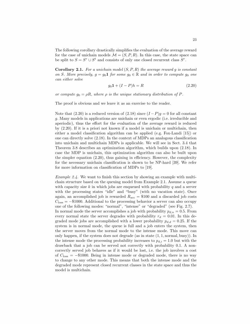
Example 2.4. We want to finish this section by showing an example with multi-chain structure based on the queuing model from Example 2.1. Assume a queuewith capacity size k in which jobs are enqueued with probability q and a serverwith the processing states “idle” and “busy” (with no vacation state). Onceagain, an accomplished job is rewarded Racc = $100 and a discarded job costsCloss = −$1000. Additional to the processing behavior a server can also occupyone of the following modes: “normal”, “intense” or “degraded” (see Fig. 2.7).In normal mode the server accomplishes a job with probability pd,n = 0.5. Fromevery normal state the server degrades with probability rd = 0.01. In this de-graded mode jobs are accomplished with a lower probability pd,d = 0.25. If thesystem is in normal mode, the queue is full and a job enters the system, thenthe server moves from the normal mode to the intense mode. This move canonly happen, if the system does not degrade (as in state (1, 1,normal,busy)). Inthe intense mode the processing probability increases to pd,i = 1.0 but with thedrawback that a job can be served not correctly with probability 0.1. A non-correctly served job behaves as if it would be lost, i.e. the job involves a costof Closs = −$1000. Being in intense mode or degraded mode, there is no wayto change to any other mode. This means that both the intense mode and thedegraded mode represent closed recurrent classes in the state space and thus themodel is multichain.
24
0,0,normal
idle
0,1,normalbusy
1,1,normalbusy
0,0,intense
idle
0,1,intense
busy
1,1,intense
busy
0,0,degraded
idle
0,1,degraded
busy
1,1,degraded
busy
1 2 3
4 5 6
7 8 9
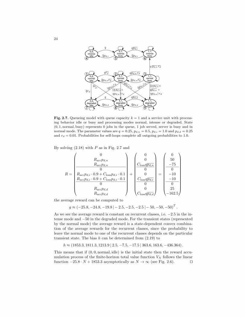
Fig. 2.7. Queueing model with queue capacity k = 1 and a service unit with process-ing behavior idle or busy and processing modes normal, intense or degraded. State(0, 1, normal, busy) represents 0 jobs in the queue, 1 job served, server is busy and innormal mode. The parameter values are q = 0.25, pd,n = 0.5, pd,i = 1.0 and pd,d = 0.25and rd = 0.01. Probabilities for self-loops complete all outgoing probabilities to 1.0.
By solving (2.18) with P as in Fig. 2.7 and
R =
0Raccpd,nRaccpd,n
0Raccpd,i · 0.9 + Closspd,i · 0.1Raccpd,i · 0.9 + Closspd,i · 0.1
0Raccpd,dRaccpd,d
+
00
Clossqpd,n00
Clossqpd,i00
Clossqpd,d
=
050−75
0−10−10
025
−162.5
the average reward can be computed to
g ≈ (−25.8,−24.8,−19.8 − 2.5,−2.5,−2.5 − 50,−50,−50)T.
As we see the average reward is constant on recurrent classes, i.e. −2.5 in the in-tense mode and −50 in the degraded mode. For the transient states (representedby the normal mode) the average reward is a state-dependent convex combina-tion of the average rewards for the recurrent classes, since the probability toleave the normal mode to one of the recurrent classes depends on the particulartransient state. The bias h can be determined from (2.19) to
h ≈ (1853.3, 1811.3, 1213.9 2.5,−7.5,−17.5 363.6, 163.6,−436.364) .
This means that if (0, 0,normal, idle) is the initial state then the reward accu-mulation process of the finite-horizon total value function VN follows the linearfunction −25.8 ·N + 1853.3 asymptotically as N →∞ (see Fig. 2.6). ut
25
3 Markov Decision Processes
This section is devoted to Markov Decision Processes with discrete time. Section3.1 provides the necessary definitions and terminology, and Sect. 3.2 introducesthe discounted reward measure as the first optimization criterion. We presentits most important properties and two standard methods (value iteration andpolicy iteration) for computing the associated optimal value function. Depend-ing on the reader’s interest, one or both of the following two subsections may beskipped: Stochastic Shortest Path Problems, the topic of Sect. 3.3, are specialMDPs together with the infinite-horizon total reward measure as optimizationcriterion. The final subsection (Sect. 3.4) addresses the optimization of the aver-age reward measure for MDPs, where we involve the bias into the computationof the average-optimal value function.
3.1 Preliminaries
We first state the formal definition of an MDP and then describe its executionsemantics. Roughly speaking, an MDP extends the purely stochastic behavior ofa DTMRM by introducing actions, which can be used in order to control statetransitions.
Definition 3.1. A discrete-time Markov Decision Process (MDP) is astructureM = (S,Act, e, P,R), where S is the finite state space, Act 6= ∅ a finiteset of actions, e : S → 2Act \ ∅ the action-enabling function, P : S×Act→ D(S)an action-dependent transition function and R : S × Act × S → R the action-dependent reward function. We denote P (s, a, s′) := (P (s, a))(s′).
From a state s ∈ S an enabled action a ∈ e(s) must be chosen which inducesa probability distribution P (s, a) over S to target states. If a transition to s′
takes place then a reward R(s, a, s′) is gained and the process continues in s′.In analogy to DTMRMs we denote R(s, a) :=
∑s′∈S P (s, a, s′)R(s, a, s′) as the
expected reward that is gained when action a has been chosen and a transitionfrom state s is performed. The mechanism which chooses an action in every stateis called a policy. In the theory of MDPs there are several possibilities to definepolicies. In this tutorial, we restrict to the simplest type of policy.
Definition 3.2. A policy is a function π : S → Act with π(s) ∈ e(s) for alls ∈ S. Define Π ⊆ ActS as the set of all policies.
A policy π of an MDPM resolves the non-deterministic choice between actionsand thus reduces M into a DTMRM Mπ := (S, Pπ, Rπ), where
Pπ(s, s′) := P (s, π(s), s′) and Rπ(s, s′) := R(s, π(s), s′).
Remark 3.1. In the literature one often finds more general definitions of policiesin which the choice of an action a in state s does not only depend on the currentstate s but also
26
– on the history of both the state process and the previously chosen actionsand
– can be randomized, i.e. the policy prescribes for each state s a probabilitydistribution π(s) ∈ D(e(s)) over all enabled actions and action a is chosenwith probability (π(s))(a).
The policy type as in Definition 3.2 is often referred to “stationary Markoviandeterministic”. Here, deterministic is in contrast to randomized and means thatthe policy assigns a fixed action instead of some probability distribution overactions. A policy is Markovian, if the choice of the action does not depend on thecomplete history but only on the current state and point in time of the decision.A Markovian policy is stationary, if it takes the same action a everytime it visitsthe same state s and is thus also independent of time. For simplicity we stick tothe type of stationary Markovian deterministic policies as in Definition 3.2 sincethis is sufficient for the MDP optimization problems we discuss in this tutorial.The more general types of policies are required if e.g. the target function to beoptimized is of a finite-horizon type or if additional constraints for optimizationare added to the MDP model (see also Remark 3.3).
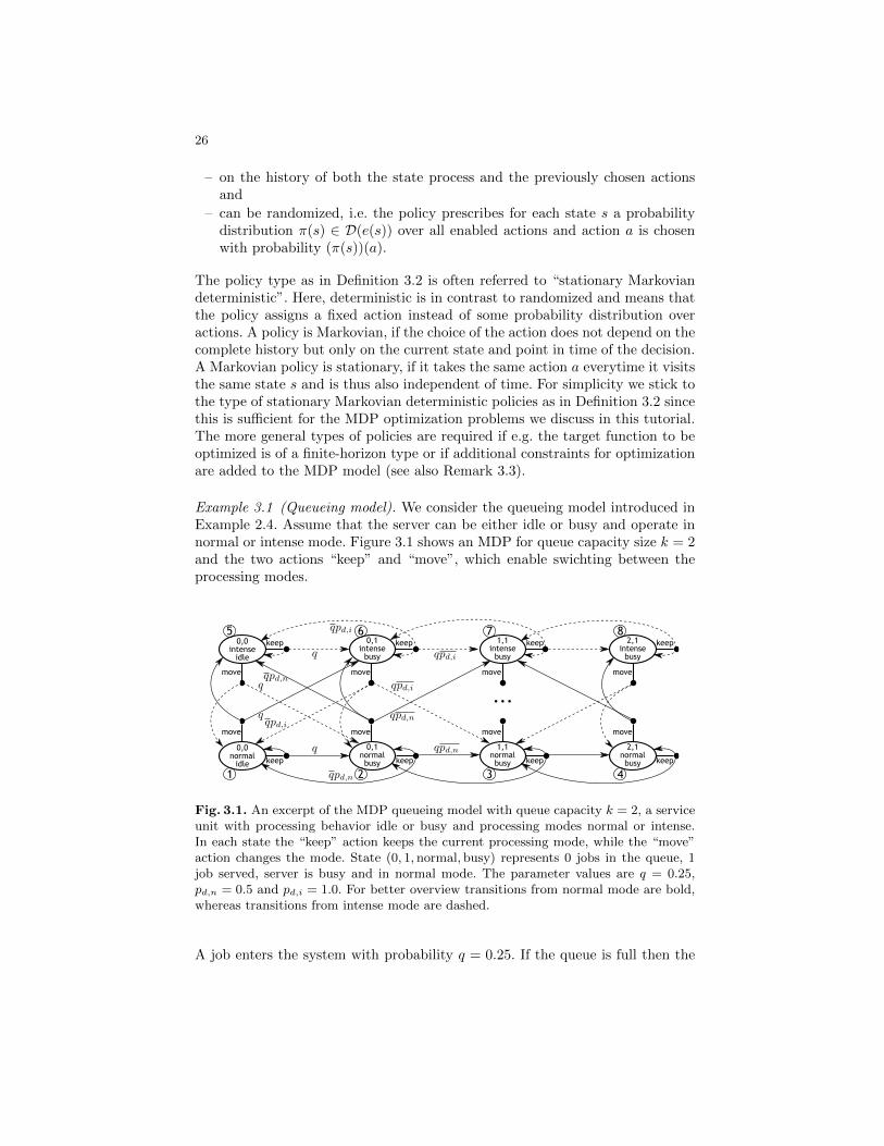
Example 3.1 (Queueing model). We consider the queueing model introduced inExample 2.4. Assume that the server can be either idle or busy and operate innormal or intense mode. Figure 3.1 shows an MDP for queue capacity size k = 2and the two actions “keep” and “move”, which enable swichting between theprocessing modes.
0,0normalidle
0,1normalbusy
1,1normalbusy
move
keep keep keep
2,1normalbusy keep
0,0intenseidle
0,1intensebusy
1,1intensebusy
move
keep 2,1intensebusy
move movemove
move
keep keep keep
move move
...
5 6 7
1 2 3 4
8
Fig. 3.1. An excerpt of the MDP queueing model with queue capacity k = 2, a serviceunit with processing behavior idle or busy and processing modes normal or intense.In each state the “keep” action keeps the current processing mode, while the “move”action changes the mode. State (0, 1, normal, busy) represents 0 jobs in the queue, 1job served, server is busy and in normal mode. The parameter values are q = 0.25,pd,n = 0.5 and pd,i = 1.0. For better overview transitions from normal mode are bold,whereas transitions from intense mode are dashed.
A job enters the system with probability q = 0.25. If the queue is full then the
27
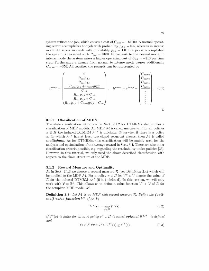
system refuses the job, which causes a cost of Closs = −$1000. A normal operat-ing server accomplishes the job with probability pd,n = 0.5, whereas in intensemode the server succeeds with probability pd,i = 1.0. If a job is accomplishedthe system is rewarded with Racc = $100. In contrast to the normal mode, inintense mode the system raises a higher operating cost of Cint = −$10 per timestep. Furthermore a change from normal to intense mode causes additionallyCmove = −$50. All together the rewards can be represented by
Rkeep =
0Raccpd,nRaccpd,n
Raccpd,n + Clossqpd,nCint
Raccpd,i + Cint
Raccpd,i + Cint
Raccpd,i + Clossqpd,i + Cint
, Rmove = Rkeep +
Cmove
Cmove
Cmove
Cmove
0000
. (3.1)
ut
3.1.1 Classification of MDPsThe state classification introduced in Sect. 2.1.2 for DTMRMs also implies aclassification of MDP models. An MDPM is called unichain, if for all policiesπ ∈ Π the induced DTMRM Mπ is unichain. Otherwise, if there is a policyπ, for which Mπ has at least two closed recurrent classes, then M is calledmultichain. As for DTMRMs, this classification will be mainly used for theanalysis and optimization of the average reward in Sect. 3.4. There are also otherclassification criteria possible, e.g. regarding the reachability under policies [33].However, in this tutorial, we only need the above described classification withrespect to the chain structure of the MDP.
3.1.2 Reward Measure and OptimalityAs in Sect. 2.1.3 we choose a reward measure R (see Definition 2.4) which willbe applied to the MDP M. For a policy π ∈ Π let V π ∈ V denote the value ofR for the induced DTMRM Mπ (if it is defined). In this section, we will onlywork with V = RS . This allows us to define a value function V ∗ ∈ V of R forthe complete MDP model M.
Definition 3.3. Let M be an MDP with reward measure R. Define the (opti-mal) value function V ∗ of M by
V ∗(s) := supπ∈Π
V π(s), (3.2)
if V ∗(s) is finite for all s. A policy π∗ ∈ Π is called optimal if V π∗
is definedand
∀s ∈ S ∀π ∈ Π : V π∗(s) ≥ V π(s). (3.3)
28
Note that in the definition of V ∗ the supremum is taken in a state-dependentway. Furthermore, since the state and action spaces are finite, the policy spaceΠ is finite as well. Therefore, the supremum in the above definition is indeed amaximum. It follows that if for all π ∈ Π the value V π(s) is defined and finitethen V ∗(s) is also finite for all s.In case R is the infinite-horizon total reward measure, we allow in contrastto Definition 2.5 the value V π(s) to converge improperly to −∞. Taking thesupremum in (3.2) doesn’t care of this kind of convergence, if there is at leastone policy providing a finite value V π(s). The same holds for (3.3) since hereV π∗
has to exist in the sense of Definition 2.5 (and thus be finite).Note further that through the definition of an optimal policy it is not clear if anoptimal policy π∗ exists, since π∗ has to fulfill the inequality in (3.3) uniformlyover all states. Definition 3.3 gives rise to the following natural question: Underwhich conditions does an optimal policy π∗ exist and how is it related to theoptimal value V ∗? These questions will be answered in the following subsections.
3.2 Discounted Reward Measure
We first address the above mentioned questions in the case of the discountedreward measure with discount factor γ ∈ (0, 1), since this measure is analyticallysimpler to manage than the infinite-horizon or the average reward measure.For motivation, let us first provide some intuition on the optimization problem.Assume we have some value function V : S → R and we want to check whether Vis optimal or alternatively in what way can we modify V in order to approach theoptimal value V ∗. When in some state s one has a choice between enabled actionsa ∈ e(s), then for each of these actions one can perform a look-ahead step andcomputeQ(s, a) := R(s, a)+γ
∑s′∈S P (s, a, s′)V (s′). The valueQ(s, a) combines
the reward R(s, a) gained for the performed action and the expectation over thevalues V (s′) for the transition to the target state s′ induced by action a. If nowQ(s, a′) > V (s) for some a′ ∈ e(s) then clearly one should improve V by theupdated value V (s) := Q(s, a′) or even better choose the best improving actionand set V (s) := maxa∈e(s)Q(s, a). This update procedure can be formalized byconsidering the Bellman operator T : RS → RS which assigns to each valuefunction V ∈ RS its update T V := T (V ) ∈ RS defined by
(T V )(s) := maxa∈e(s)
R(s, a) + γ
∑s′∈S
P (s, a, s′)V (s′)
.
Note that T is a non-linear operator on the vector space RS , since it involvesmaximization over actions. If we proceed iteratively, a sequence of improvingvalue functions V is generated and the hope is that this sequence convergencesto the optimal value function V ∗. In case V is already optimal, there should beno strict improvement anymore possible. This means that for every state s thevalue V (s) is maximal among all updates Q(s, a), a ∈ e(s) on V (s), i.e.
V (s) = maxa∈e(s)
R(s, a) + γ
∑s′∈S
P (s, a, s′)V (s′)
. (3.4)
29
This non-linear fixed-point equation V = T V is also known as the Bellmanoptimality equation and we have to solve it, if we want to detemine V ∗.The following Theorem 3.1 establishes results on existence and uniqueness ofsolutions to this equation. Furthermore, it also creates a connection between theoptimal value function V ∗ and optimal policies π∗.
Theorem 3.1 (Existence Theorem). Consider an MDP (S,Act, e, P,R) andthe discounted reward measure with discount factor γ ∈ (0, 1).
(i) There exists an optimal value (V γ)∗
which is the unique fixed point of T ,i.e. the Bellman optimality equation holds:
(V γ)∗
= T (V γ)∗. (3.5)
(ii) There exists an optimal policy π∗ and it holds that (V γ)π∗
= (V γ)∗.
(iii) Every optimal policy π∗ can be derived from the optimal value (V γ)∗
by
π∗(s) ∈ argmaxa∈e(s)
R(s, a) + γ
∑s′∈S
P (s, a, s′) (V γ)∗
(s′)
.
The complete proof can be found in [33]. The key ingredient for this proof relieson the following lemma, which provides an insight into the analytical propertiesof the Bellman operator T .
Lemma 3.1. (i) T is monotonic, i.e. if U(s) ≤ V (s) for all s ∈ S then(T U)(s) ≤ (T V )(s) for all s.
(ii) T is a contraction with respect to the maximum norm ||V || := maxs∈S |V (s)|,i.e. there exists q ∈ R with 0 ≤ q < 1 such that
||T U − T V || ≤ q||U − V ||.
The constant q is called Lipschitz constant and one can choose q := γ.
Remark 3.2. Lemma 3.1(ii) allows to apply the Banach fixed point theorem onthe contraction T which ensures existence and uniqueness of a fixed point Vfix.Furthermore the sequence
Vn+1 := T Vn (3.6)
converges to Vfix for an arbitrary initial value function V0 ∈ RS . From the mono-tonicity property of T it can be shown that the sequence in (3.6) also convergesto the optimal value (V γ)
∗and thus Vfix = (V γ)
∗.
Writing (3.5) in component-wise notation yields exactly the Bellman optimalityequation (3.4) as motivated, for which (V γ)
∗is the unique solution. Note that
(V γ)∗
is defined in (3.2) by a maximization over the whole policy space Π, i.e.for each state s all policies π ∈ Π have to be considered in order to establishthe supremum. In contrast, the Bellman optimality equation reduces this globaloptimization task into a local state-wise optimization over the enabled actionsa ∈ e(s) for every s ∈ S. Note also that from Theorem 3.1 one can deduce that
30
T ((V γ)π∗
) = (V γ)π∗
, such that an optimal policy π∗ can be also considered asa “fixed-point” of the Bellman operator T . However, an optimal policy does notneed to be unique.
From the Bellman equation (3.4) several algorithms based on fixed-point itera-tion can be derived which can be used in order to compute the optimal policytogether with its value function. The following value iteration algorithm is basedon (3.6). Its proof can be found in the Appendix on page 82.
Theorem 3.2 (Value Iteration). For an arbitrary initial value function V0 ∈RS define the sequence of value functions
Vn+1(s) := (T Vn) (s) = maxa∈e(s)
R(s, a) + γ
∑s′∈S
P (s, a, s′)Vn(s′)
.
Then Vn converges to (V γ)∗. As a termination criterion choose ε > 0 and con-
tinue iterating until ||Vn+1 − Vn|| < 1−γ2γ ε and let
πε(s) ∈ argmaxa∈e(s)
R(s, a) + γ
∑s′∈S
P (s, a, s′)Vn+1(s′)
. (3.7)
Then ||V πε − (V γ)∗ || < ε.
The value iteration algorithm iterates on the vector space RS of value functions.From an arbitrary value function an improving policy can be generated by (3.7).In contrast, the following policy iteration algorithm iterates on the policy spaceΠ. From a policy π its value can be generated the other way round by solving asystem of linear equations.
Theorem 3.3 (Policy Iteration). Let π0 ∈ Π be an initial policy. Define thefollowing iteration scheme.
1. Policy evaluation: Compute the value V πn of πn by solving
(I − γPπn)V πn = Rπn
and define the set of improving actions
An+1(s) := argmaxa∈e(s)
R(s, a) + γ
∑s′∈S
P (s, a, s′)V πn(s′)
.
Termination: If πn(s) ∈ An+1(s) for all s then πn is an optimal policy.2. Policy improvement: Otherwise choose an improving policy πn+1 such
that πn+1(s) ∈ An+1(s) for all s ∈ S.
The sequence of values V πn is non-decreasing and policy iteration terminateswithin a finite number of iterations.
31
Proof. By definition of πn+1 it holds for all s that
V πn+1(s) = maxa∈e(s)
R(s, a) + γ
∑s′∈S
P (s, a, s′)V πn(s′)
≥ R(s, πn(s)) + γ
∑s′∈S
P (s, πn(s), s′)V πn(s′) = V πn(s).
Since there are only finitely many policies and the values V πn are non-decreasing,policy iteration terminates in a finite number of iterations. Clearly, if πn(s) ∈An+1(s) for all s then πn is optimal, since
V πn(s) = maxa∈e(s)
R(s, a) + γ
∑s′∈S
P (s, a, s′)V πn(s′)
= (T V πn) (s).
The conclusion follows by Theorem 3.1. ut
Both presented algorithms value iteration and policy iteration create a converg-ing sequence of value functions. For value iteration we mentioned in Remark 3.2that the generated sequence Vn+1 = T Vn converges to the fixed point of T whichis also the global optimal value (V γ)
∗of the MDP since T is monotonic. Same
holds for the sequence V πn in policy iteration, since V πn is a fixed-point of T forsome n ∈ N and thus V πn = (V γ)
∗. The convergence speed of these algorithms
is in general very slow. Value iteration updates in every iteration step the valuefunction Vn on every state. This means especially that states s that in the cur-rent iteration step do not contribute to a big improvement |Vn+1(s)− Vn(s)| intheir value will be completely updated like every other state. However, it can beshown that convergence in value iteration can also be guaranteed, if every stateis updated infinitely often [37]. Thus, one could modify the order of updates tostates regarding their importance or contribution in value improvement (asyn-chronous value iteration).Policy iteration on the other hand computes at every iteration step the exactvalue V πn of the current considered policy πn, by solving a system of linearequations. If πn is not optimal, then after improvement to πn+1 the effort forthe accurate computation of V πn is lost. Therefore, the algorithms value iterationand policy iteration just provide a foundation for potential algorithmic improve-ments. Examples for such improvements are relative value iteration, modifiedpolicy iteration or action elimination [33]. Of course, heuristics which use model-dependent meta-information can also be considered in order to provide a goodinitial value V0 or initial policy π0.Note that MDP optimization underlies the curse of dimensionality: The explo-sion of the state space induces an even worse explosion of the policy space since|Π| ∈ O
(|Act||S|
). There is a whole branch of Artificial and Computational
Intelligence, which develops learning algorithms and approximation methodsfor large MDPs (e.g. reinforcement learning [37], evolutionary algorithms [29],heuristics [28] and approximate dynamic programming [8, 10,26,27,32]).
32
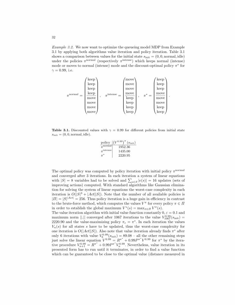
Example 3.2. We now want to optimize the queueing model MDP from Example3.1 by applying both algorithms value iteration and policy iteration. Table 3.1shows a comparison between values for the initial state sinit = (0, 0,normal, idle)under the policies πnormal (respectively πintense) which keeps normal (intense)mode or moves to normal (intense) mode and the discount-optimal policy π∗ forγ = 0.99, i.e.
πnormal =
keepkeepkeepkeepmovemovemovemove
, πintense =
movemovemovemovekeepkeepkeepkeep
, π∗ =
keepkeepkeepmovemovemovekeepkeep
.
Table 3.1. Discounted values with γ = 0.99 for different policies from initial statesinit = (0, 0, normal, idle).
policy(V 0.99
)π(sinit)
πnormal 1952.36πintense 1435.00π∗ 2220.95
The optimal policy was computed by policy iteration with initial policy πnormal
and converged after 3 iterations. In each iteration a system of linear equationswith |S| = 8 variables had to be solved and
∑s∈S |e(s)| = 16 updates (sets of
improving actions) computed. With standard algorithms like Gaussian elimina-tion for solving the system of linear equations the worst-case complexity in eachiteration is O(|S|3 + |Act||S|). Note that the number of all available policies is|Π| = |S||Act| = 256. Thus policy iteration is a huge gain in efficiency in contrastto the brute-force method, which computes the values V π for every policy π ∈ Πin order to establish the global maximum V ∗(s) = maxπ∈Π V
π(s).The value iteration algorithm with initial value function constantly 0, ε = 0.1 andmaximum norm ||.|| converged after 1067 iterations to the value V 0.99
1067(sinit) =2220.90 and the value-maximizing policy πε = π∗. In each iteration the valuesVn(s) for all states s have to be updated, thus the worst-case complexity forone iteration is O(|Act||S|). Also note that value iteration already finds π∗ afteronly 6 iterations with value V 0.99
6 (sinit) = 89.08 – all the other remaining stepsjust solve the linear equation V 0.99 = Rπ
∗+ 0.99Pπ
∗V 0.99 for π∗ by the itera-
tive procedure V 0.99n+1 = Rπ
∗+ 0.99Pπ
∗V 0.99n . Nevertheless, value iteration in its
presented form has to run until it terminates, in order to find a value functionwhich can be guaranteed to be close to the optimal value (distance measured in
33
maximum norm). Furthermore, it is a priori not known at which iteration stepthe optimization phase stops, i.e. the actions not improvable anymore. ut
Remark 3.3. (i) One of the main theorems in Markov Decision Theory states(at least for the models we consider in this tutorial) that if one searchesfor an optimal value function within the broader space of randomized andhistory-dependent policies, then an optimal policy is still stationary Marko-vian deterministic, i.e. lies within Π (see also Remark 3.1). This is the reasonwhy we stick in this introductory tutorial from beginning to the smaller pol-icy space Π.
(ii) An MDP problem can also be transformed to a linear programming problem,such that methods coming from the area of linear optimization can be appliedto solve MDPs [33]. In its generality, a linear optimization formulation alsoallows to add further constraints to the set of linear constraints inducedby the Bellman equation. An MDP model with an additional set of linearconstraints is also known as a Constrained MDP [1]. It can be shown that inthis case stationary Markovian deterministic policies π ∈ Π can indeed beoutperformed in their value by randomized and history-dependent policies.Also note that history-dependent policies can also be better then stationaryMarkovian deterministic policies in the finite-horizon case.
3.3 Stochastic Shortest Paths
We now address the problem of optimizing MDPs with respect to the infinite-horizon total reward measure. In contrast to the discounted case, the existenceof an optimal value in general can not be guaranteed. In case it exists, it isdifficult to provide convergence criteria for dynamic programming algorithms.Therefore, in literature one finds existence results and convergence criteria onlyfor special classes of MDPs with respect to this measure. In the following, weshow only one frequently used application for this type of measure.
Definition 3.4. A stochastic shortest path problem (SSP) is an MDP(S,Act, e, P,R) with an absorbing and reward-free state goal ∈ S, i.e. for allpolicies π ∈ Π it holds
Pπ(goal, goal) = 1 and Rπ(goal) = 0.
Typically, in SSPs the goal is to minimize costs and not to maximize rewards(see Definition 3.3). Of course, maximization of rewards can be transformed toa minimization of costs, where costs are defined as negative rewards. Note thatwe allow for rewards (and therefore also for costs) to have both a positive and anegative sign. In order to be consistent with the rest of this tutorial, we stick inthe following to the maximization of rewards. For being able to provide resultson the existence of optimal solutions, we have to define the notion of a properpolicy.
34
Definition 3.5. A policy π is called proper if there is m ∈ N such that underπ the goal state can be reached from every state with positive probability withinm steps, i.e.
∃m ∈ N ∀s ∈ S : (Pπ)m(s, goal) > 0.
A policy is called improper if it is not proper.
Define the Bellman operator T : RS → RS by
(T V )(s) := maxa∈e(s)
R(s, a) +
∑s′∈S
P (s, a, s′)V (s′)
.
In analogy to the discounted case it holds that T is monotonic (see Lemma 3.1).But the contraction property with respect to the maximum norm is in general notsatisfied. However, Bertsekas and Tsitsiklis proved for typical SSPs the existenceand uniqueness of optimal values and the existence of optimal policies [9, 10].
Theorem 3.4 (Existence Theorem). Consider an SSPM = (S,Act, e, P,R)with infinite-horizon total reward measure. Further assume that there exists aproper policy πp ∈ Π and for every improper policy πi there exists s ∈ S suchthat V πi∞ (s) = −∞.
(i) There exists an optimal value V ∗∞ which is the unique fixed point of T , i.eT V ∗∞ = V ∗∞.
(ii) There exists an optimal policy π∗ and it holds that V π∗
∞ = V ∗∞.(iii) Every optimal policy π∗ can be derived from the optimal value V ∗∞ by
π∗(s) ∈ argmaxa∈e(s)
R(s, a) +
∑s′∈S
P (s, a, s′)V ∗∞(s′)
.
The dynamic programming algorithms value iteration and policy iteration aspresented for discounted MDPs (Theorems 3.2 and 3.3) can be applied for SSPsin an analogous way and are shown in Theorems 3.5 and 3.6. The most importantdifference is the termination criterion in value iteration, which in contrast to thediscounted case uses a weighted maximum norm in order to measure the distancebetween the iterated values and the optimal value. The proofs for both theoremscan be found in [8, 10].
Theorem 3.5 (Value Iteration). Consider an SSP M with the assumptionsfrom Theorem 3.4. Let V0(s) be an arbitrary value function with V0(goal) = 0.Define the sequence
Vn+1(s) := (T Vn) (s) = maxa∈e(s)
R(s, a) +
∑s′∈S
P (s, a, s′)Vn(s′)
.
(i) Vn converges to V ∗.
35
(ii) If every policy is proper, then there exists ξ ∈ RS with ξ(s) ≥ 1 for all s ∈ S,such that T is a contraction with respect to the ξ-weighted maximum norm||.||ξ defined by
||V ||ξ := maxs∈S
|V (s)|ξ(s)
.
As Lipschitz constant q for contraction of T choose q := maxs∈Sξ(s)−1ξ(s) . For
a given ε > 0 stop value iteration when ||Vn+1 − Vn||ξ < 1−q2q ε and choose
πε(s) ∈ argmaxa∈e(s)
R(s, a) +
∑s′∈S
P (s, a, s′)Vn+1(s′)
.
Then ||V πε − V ∗||ξ < ε.
In the following, we want to briefly outline, how ξ(s) can be determined. Consideran arbitrary policy π. Since π is proper by assumption, the expected number oftransitions t(s) from s to goal is finite. If π is the single available policy, thentake ξ(s) := t(s). In case there are more policies available, it could be the case,that there exists another policy which enlarges for some state s the expectednumber of transitions towards goal. Thus ξ(s) can be chosen as the maximalexpected number of transitions to goal among all policies. In order to computeξ exactly, a modified SSP can be considered: Define a reward R(s, a) which actsas a counter for the number of transitions to goal, i.e. each state s 6= goal isrewarded R(s, a) := 1 independent of a ∈ e(s) and the goal state is rewarded 0.Choose ξ as the optimal solution to the induced Bellman equation:
ξ(s) = 1 + maxa∈e(s)
∑s′∈S
P (s, a, s′)ξ(s′)
for s 6= goal and ξ(goal) = 0. (3.8)
Note that if we allow improper policies πi in the termination check of Theorem3.5 then by definition of πi there is some state si from which goal is reached withprobability 0. In this case the Bellman equation (3.8) is not solvable, since anysolution ξ would imply that ξ(si) =∞. The proof for the termination criterionin Theorem 3.5 is completely analogous to the proof of Theorem 3.2 (see Ap-pendix, page 82). It holds that for every policy π the linear operator Tπ definedby TπV = Rπ + PπV is also a contraction with respect to ||.||ξ and Lipschitzconstant q as defined in Theorem 3.5.
For completeness we also state the policy iteration algorithm which is directlytransfered from the discounted case as in Theorem 3.3 by setting the discountfactor γ := 1. We omit the proof since it is analogous.
Theorem 3.6 (Policy Iteration). Let π0 ∈ Π an arbitrary initial policy. De-fine the following iteration scheme.
1. Policy evaluation: Compute the value V πn of πn by solving
(I − Pπn)V πn = Rπn with V πn(goal) = 0
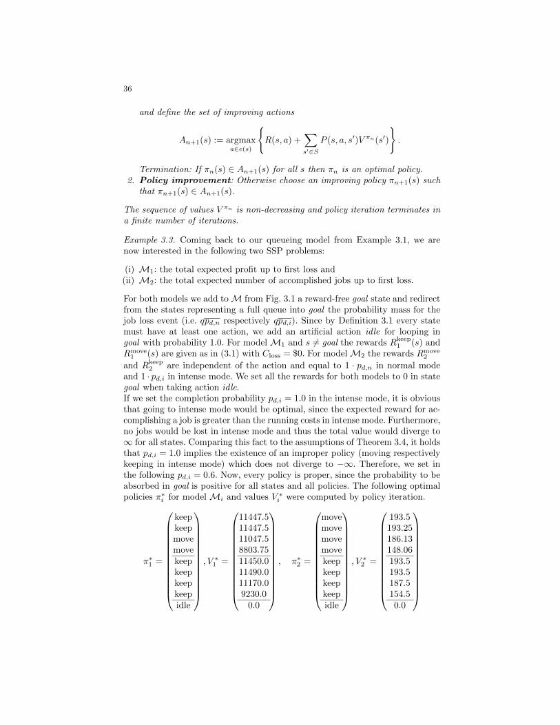
36
and define the set of improving actions
An+1(s) := argmaxa∈e(s)
R(s, a) +
∑s′∈S
P (s, a, s′)V πn(s′)
.
Termination: If πn(s) ∈ An+1(s) for all s then πn is an optimal policy.2. Policy improvement: Otherwise choose an improving policy πn+1(s) such
that πn+1(s) ∈ An+1(s).
The sequence of values V πn is non-decreasing and policy iteration terminates ina finite number of iterations.
Example 3.3. Coming back to our queueing model from Example 3.1, we arenow interested in the following two SSP problems:
(i) M1: the total expected profit up to first loss and(ii) M2: the total expected number of accomplished jobs up to first loss.
For both models we add toM from Fig. 3.1 a reward-free goal state and redirectfrom the states representing a full queue into goal the probability mass for thejob loss event (i.e. qpd,n respectively qpd,i). Since by Definition 3.1 every statemust have at least one action, we add an artificial action idle for looping ingoal with probability 1.0. For modelM1 and s 6= goal the rewards Rkeep
1 (s) andRmove
1 (s) are given as in (3.1) with Closs = $0. For modelM2 the rewards Rmove2
and Rkeep2 are independent of the action and equal to 1 · pd,n in normal mode
and 1 · pd,i in intense mode. We set all the rewards for both models to 0 in stategoal when taking action idle.If we set the completion probability pd,i = 1.0 in the intense mode, it is obviousthat going to intense mode would be optimal, since the expected reward for ac-complishing a job is greater than the running costs in intense mode. Furthermore,no jobs would be lost in intense mode and thus the total value would diverge to∞ for all states. Comparing this fact to the assumptions of Theorem 3.4, it holdsthat pd,i = 1.0 implies the existence of an improper policy (moving respectivelykeeping in intense mode) which does not diverge to −∞. Therefore, we set inthe following pd,i = 0.6. Now, every policy is proper, since the probability to beabsorbed in goal is positive for all states and all policies. The following optimalpolicies π∗i for model Mi and values V ∗i were computed by policy iteration.
π∗1 =
keepkeepmovemovekeepkeepkeepkeepidle
, V ∗1 =
11447.511447.511047.58803.7511450.011490.011170.09230.0
0.0
, π∗2 =
movemovemovemovekeepkeepkeepkeepidle
, V ∗2 =
193.5193.25186.13148.06193.5193.5187.5154.50.0
37
Note also that if value iteration is applied, then the maximal expected numberξ(s) of transitions from s to goal is given as the optimal solution of the SSP in(3.8) by
ξ = (790.0, 785.0, 752.5, 596.25, 790.0, 786.0, 758.0, 622.0, 0.0) .
Therefore, the Lipschitz constant q = 0.9988 can be chosen, which is very highand makes value iteration in the ξ-weighted maximum norm terminating verylate. Thus, the termination criterion in the ξ-weighted norm is a theoreticalguarantee, but in general not applicable in practice. ut
We finish the section on the infinite-horizon total reward measure with an out-look to other typical total value problems discussed in [33].
Remark 3.4. Beside SSPs one also often considers the following model types:
(i) Positive models: For each state s there exists a ∈ e(s) with R(s, a) ≥ 0and for all policies π the value V π(s) <∞ (this assumption can be relaxed).
(ii) Negative models: For each state s all rewards R(s, a) ≤ 0 and there existsa policy π with V π(s) > −∞ for all s.
In a positive model the goal is to maximize the accumulation of positive rewardstowards∞. The model assumptions make this possible, since in every state thereis at least one non-negative reward available and the accumulation does notdiverge to ∞. In contrast, the goal in a negative model is to maximize negativerewards, i.e. to minimize costs towards 0. The value iteration algorithm for bothmodels is the same as in Theorem 3.5, but without convergence criteria. Thepolicy iteration algorithm however differs from the policy iteration for SSPs. Ina positive model, the initial policy π0 has to be chosen suitable with Rπ0(s) ≥ 0.Furthermore, in the policy evaluation phase the solutions to the linear equationV = Rπ +PπV for a policy π spans up a whole subspace of RS . In this subspacea minimal solution Vmin ≥ 0 has to be chosen in order to perform the policyimprovement phase on Vmin. In contrast, in a negative model, the initial policyπ0 has to fulfill V π0 > −∞ and in the policy evaluation phase the maximalnegative solution has to be computed. Puterman shows in [33] that for bothmodel types value iteration converges for V0 = 0, but convergence of policyiteration is only assured for positive models.
3.4 Average Reward Measure
We now come to the final part of the MDP section, which is devoted to theoptimization of the average reward measure. As a reminder, let us consider for themoment a discrete-time Markov Reward Model M = (S, P,R). From Theorem2.4 we know that if g is the average reward of M then g = Pg. On the otherhand, the average reward cannot be uniquely determined by this single equation.Any solution u to u = Pu defines a further linear equation u+ (I − P )v = R inv. If this additional equation is solvable, then and only then u = g is the average
38
reward. In this case the bias h is one of the possible solutions to the secondequation (and unique modulo ker(I − P )). We write both of these equations inthe fixed-point form
g = Pg and h = (R+ Ph)− g. (3.9)
Also remember, that ifM is unichain, then by Corollary 2.1 the equation g = Pgcan be simplified to “g is constant”.We are concerned in this section with the optimization of the average rewardfor an MDP M = (S,Act, e, P,R). Surely, every policy π ∈ Π of M induces aDTMRMMπ = (S, Pπ, Rπ) and we can compute for each π the average rewardgπ as described above. By Definition 3.3 the optimal average value function isg∗(s) = supπ∈Π g
π(s) and in case an optimal policy π∗ exists then gπ∗(s) ≥ gπ(s)
for all s and all π. In analogy to the previous sections, it is possible to establishBellman equations which reduce the global optimization task over all policiesπ ∈ Π to a local state-wise search over actions e(s) for all states s. Since theformal derivation of these Bellman equations is slightly involved, we just statethem and refer for proof to [33]. Define for each of the two linear fixed-pointequations in (3.9) the Bellman operators Tav : RS → RS and T gbias : RS → RS(parametrized by g ∈ RS) as follows:
(Tavg)(s) := maxa∈e(s)
∑s′∈S
P (s, a, s′)g(s′)
(3.10)
(T gbiash)(s) := maxa∈eg(s)
R(s, a) +
∑s′∈S
P (s, a, s′)h(s′)
− g(s) (3.11)
where eg(s) :=
a ∈ e(s) | g(s) =
∑s′∈S
P (s, a, s′)g(s′)
.
The corresponding Bellman optimality equations for the average reward are justthe fixed-point equations of these operators and read as
g(s) = maxa∈e(s)
∑s′∈S
P (s, a, s′)g(s′)
(3.12)
h(s) = maxa∈eg(s)
R(s, a) +
∑s′∈S
P (s, a, s′)h(s′)
− g(s). (3.13)
Equations (3.12) and (3.13) are referred to as the first and the second optimalityequation. In order to provide an intuition for these equations, assume for themoment that there is an optimal policy π∗ with gπ
∗= g∗ and moreover that
the MDP M is unichain. In this case, the average reward gπ(s) is a constantfunction for any policy π and thus the first optimality equation does not yieldany further restriction since it is satisfied for every constant function g. Only thesecond equation takes the reward values R(s, a) into account that are needed in
39
order determine their average. For each policy π the average reward gπ and thebias hπ satisfy
hπ(s) = (Rπ(s)− gπ(s)) +∑s′∈S
Pπ(s, s′)hπ(s′),
i.e. the bias hπ is the total value function for the DTMRM with average-correctedrewards Rπ(s) − gπ(s). Since this holds especially for π = π∗, the second op-timality equation can be seen as a Bellman equation for maximizing the totalvalue function for the MDP model with rewards R(s, a)− g∗(s). In other words,if π is an arbitrary policy then the DTMRM with rewards R(s, π(s)) − g∗(s)has a total value function if and only if g∗(s) is the average reward for theDTMRM (S, Pπ, Rπ) and this holds especially for π = π∗. In case M is mul-tichain, then gπ
∗(s) is only constant on recurrent classes of Mπ∗ , whereas if
s is transient then gπ∗(s) is a weighted sum over all those average rewards on
recurrent classes. This means that gπ∗
has to fulfill gπ∗
= Pπ∗gπ∗
in additionand thus gπ
∗is a solution to the first optimality equation. Since both Bellman
equations are nested and have to be satisfied simultaneously, it is possible toreduce the set of actions e(s) in the second equation to the maximizing ac-tions eg(s) = argmaxa∈e(s)
∑s′∈S P (s, a, s′)g(s′)
for a solution g of the first
equation. Note that in case of unichain models it holds that eg(s) = e(s) for all s.
The following theorem formalizes the explanations in the motivation above andconnects the Bellman equations to the optimal value and optimal policies. Werefer for proof to [33].
Theorem 3.7 (Existence Theorem). Consider an MDPM=(S,Act, e, P,R)with average reward measure.
(i) The average optimal value function g∗ is a solution to (3.12), i.e g∗ = Tavg∗.
For g = g∗ there exists a solution h to (3.13), i.e. h = T g∗
biash. If g and h aresolutions to (3.12) and (3.13) then g = g∗.
(ii) There exists an optimal policy π∗ and it holds that gπ∗
= g∗.(iii) For any solution h to (3.13) with g = g∗ an optimal policy π∗ can be derived
from
π∗(s) ∈ argmaxa∈eg∗ (s)
R(s, a) +
∑s′∈S
P (s, a, s′)h(s′)
.
As a special case of part (iii) in this theorem it holds that if for a policy π theaverage reward gπ and the bias hπ solve the Bellman optimality equations, thenπ is optimal. In contrast to the discounted and total reward cases, the conversedoes not hold. This means that if a policy π is optimal then gπ and hπ are notnecessary solutions to the Bellman equations.The following policy iteration algorithm, can be applied in order to compute theoptimal average reward g∗ as well as an optimal policy π∗. A proof can be foundin [33].
40
Theorem 3.8 (Policy Iteration). Let π0 ∈ Π be an initial policy. Define thefollowing iteration scheme:
1. Policy evaluation: Compute a solution (gπn , hπn , w)T
toI − Pπn 0 0I I − Pπn 00 I I − Pπn
gπnhπn
w
=
0Rπn
0
. (3.14)
Define
Gn+1(s) := argmaxa∈e(s)
∑s′∈S
P (s, a, s′)gπn(s′)
.
2. Policy improvement: If πn(s) 6∈ Gn+1(s) for some s then choose an im-proving policy πn+1 with πn+1(s) ∈ Gn+1(s) and go to the policy evaluationphase. Otherwise if πn(s) ∈ Gn+1(s) for all s then define
Hn+1(s) := argmaxa∈egπn (s)
R(s, a) +
∑s′∈S
P (s, a, s′)hπn(s′)
.
If πn(s) 6∈ Hn+1(s) for some s then choose an improving policy πn+1 suchthat πn+1(s) ∈ Hn+1(s) and go to the policy evaluation phase.Termination: If πn(s) ∈ Hn+1(s) for all s then πn is an optimal policy.
The values gπn are non-decreasing and policy iteration terminates in a finitenumber of iterations with an optimal policy πn and optimal average value gπn .
Note that (3.14) corresponds to (2.19) instead of (2.18) for the following reason:For each policy π (2.18) provides a unique solution gπ to the average reward, butin general the bias hπ cannot be uniquely determined. Policy iteration can beassured to converge if the bias hπn is computed for each iterated policy πn [33].As described in Remark 2.4(iii) this can be done by solving (2.19), i.e. the equa-tion v + (I − Pπn)w = 0 in addition to (2.18) for which v = hπn is the uniquesolution. There are also other possibilities to assure convergence of policy it-eration by solving only (2.18) and fixing a scheme that chooses a solution v tog+(I−P )v = R in order to prevent cycles in policy iteration (see Remark 2.4(ii)).
Before showing the application of policy iteration on our queueing model runningexample, we first state the following remark regarding some algorithmic aspects.
Remark 3.5. (i) During policy iteration the action set egπn(s)
can be replacedby the whole action set e(s) – this leads to the so-called modified optimal-ity equations. The convergence and the optimality of the solution in policyiteration are not influenced by this replacement.
(ii) In the policy improvement phase, there are two jumps to the policy evalua-tion phase, which represent two nested cycles of evaluation and improvementphases. First, a policy πn has to be found, which solves the first optimality
41
equation. Then in a nested step, πn is tested on the second optimality equa-tion. If πn can be improved by a better policy πn+1 with actions from Hn+1
then πn+1 has to be sent back to the first evaluation and improvement cycleuntil it again solves the first optimality equation, and so on.
(iii) As already mentioned in the introducing motivation, if it is a priori knownthat the MDP is unichain, i.e. for all policies there is only one closed re-current class of states, then the optimal average reward is constant and thefirst optimality equation is automatically satisfied (see Corollary 2.1). Thisreduces the complexity of policy iteration, since only the second optimalityequation has to be considered for optimization.
(iv) We skip the value iteration algorithm in this tutorial since it is exactlythe same as for the discounted case (Theorem 3.2) with γ := 1. It can beproven that the sequence Vn+1−Vn converges to the optimal average rewardg∗, if for every (optimal) policy the transition matrix is aperiodic [33]. Theaperiodicity constraint is not a restriction, since every periodic DTMRM canbe made aperiodic, by inserting self-loops with strictly positive probabilityfor every state. (The reward function has to be transformed accordingly.)However, [33] presents a termination criterion for value iteration only formodels with g∗(s) constant for all s (e.g. unichain models).
Example 3.4. Consider the queueing MDP model from Example 3.1. We wantto compute the optimal average value function for the queueing model withparameters q = 0.25, pd,n = 0.5 and pd,i = 1.0 and the reward structure asspecified in (3.1). Note that the model is multichain, since the policy that takesthe action keep in every state induces a DTMRM with two recurrent classes.Policy iteration converges after three iterations (with initial policy π0 whichkeeps in normal mode or moves to it from intense mode) and results in thefollowing optimal policy π∗, optimal average value g∗ = gπ
∗and bias hπ
∗:
π∗ =
keepkeepkeepmovemovemovekeepkeep
, gπ
∗=
22.722.722.722.722.722.722.722.7
, hπ
∗=
−49.441.395.338.7−59.440.6130.3220.0
.
Thus, the optimal policy induces a DTMRM that is unichain with constantoptimal average reward 22.7. The finite-horizon total value function V π
∗
N fromstate (0, 0,normal, idle) increases asymptotically with 22.7 ·N −49.4 as N →∞.
ut
We conclude the MDP section by a further remark, which presents a short out-look on other optimization criteria that are applicable for MDPs.
42
Remark 3.6. The average reward considers reward accumulation in the long-run. Therefore, it is not very sensitive in the selection between policies with thesame average reward: If two policies have the same long-run average reward butdifferent short-run rewards, then one would prefer among all policies with thesame average reward such a policy that also maximizes the short-run rewardaccumulation. This idea leads to the so-called bias (or more general n-biasor n-discount) optimization criteria, which belongs to the class of sensitivediscount optimality criteria. In more detail, policies π ∈ Π are comparedregarding their Laurent series expansions (2.15)
(V γ)π
= a−1gπ + a0H
πRπ + a1 (Hπ)2Rπ + . . . ,
where ai are constants (depending only on γ) and HπRπ = hπ is the bias, whichrepresents the excess in reward accumulation up to steady-state. Now if a subsetof policies Π∗−1 ⊆ Π maximize gπ then this subset can be further refined to areduced subset Π∗0 ⊆ Π∗−1 by maximizing the bias hπ for π ∈ Π∗−1 in additionto the average reward gπ. If Π∗0 still consists of more then one policy, then onecan proceed iteratively and compare the higher order n-bias terms sequentially.Note that the n-bias reward measure specifies the vector space V of value func-tions as V =
V : S → Rn+1
and values can be compared in Definition 3.3 by
lexicographic order.The most sensitive optimization criterion is the Blackwell optimality crite-rion, which selects a policy π∗, such that the entire Laurent series expansion(i.e. the complete discounted value) is maximal among the discounted values forall policies and for all discount factors high enough, i.e.
∃γ∗ ∈ [0, 1) ∀γ ∈ [γ∗, 1) ∀π ∈ Π : (V γ)π∗ ≥ (V γ)
π.
It can be shown, that Blackwell optimal policies exist and a Blackwell optimalpolicy is n-bias optimal for all n [33]. Furthermore, such a policy can be computedby proceeding with the policy space reduction as described above until some Π∗nconsists of only one policy, which is Blackwell optimal (or if n ≥ |S|−2 then Π∗nis a set of Blackwell optimal policies).
43
4 Continuous Time Markov Reward Models
In both DTMRMs and MDPs time is discrete, i.e. it proceeds in a step by stepmanner. However, this is unrealistic for many applications – one rather wishesto work with a continuous notion of time. Therefore, in this and the followingsection, we study continuous-time models. Since we stick to the principle of mem-orylessness, it will turn out that the state sojourn times follow an exponentialdistribution (as opposed to the geometrically distributed sojourn times in thediscrete-time setting).
4.1 Preliminaries
Definition 4.1. A continuous-time Markov chain (CTMC) is a structureM = (S,Q) with finite state space S and generator function Q : S×S → R suchthat Q(s, s′) ≥ 0 for s′ 6= s and
∑s′∈S Q(s, s′) = 0 for all s. A continuous-
time Markov Reward Model (CTMRM) is a structure (S,Q, i, r) whichenhances a CTMC (S,Q) by a reward structure consisting of an impulse rewardfunction i : S × S → R for transitions with i(s, s) = 0 for all s ∈ S and a ratereward function r : S → R for states.
From state s ∈ S each quantity Q(s, s′) with s′ 6= s defines an event which occursafter a random amount of time τs,s′ ∈ R ∪ ∞ to trigger. If Q(s, s′) > 0 thenτs,s′ is exponentially distributed with rate Q(s, s′) and otherwise if Q(s, s′) = 0then we set τs,s′ :=∞. For a fixed s ∈ S all these times τs,s′ are independent andconcurrently enabled. Therefore, they define a race among each other and onlythat τs,s′0 which triggers first, within a finite amount of time (i.e. τs,s′0 ≤ τs,s′
for all s′ ∈ S), wins the race. In this case the system performs a transitionfrom s to s′0 6= s and collects the impulse reward i(s, s′0) ∈ R. The time τsthat the system resides in state s (up to transition) is called the sojourn timeand fulfills τs = min τs,s′ | s′ 6= s. While the system is in state s the ratereward r(s) is accumulated proportionally to the sojourn time τs. Thus, theaccumulated reward in s for the sojourn time including the transition to states′0 is given by R(s) := i(s, s′0) + r(s)τs. The quantity E(s) :=
∑s′ 6=sQ(s, s′) is
called the exit rate in state s and by definition of the generator function Q itholds that E(s) = −Q(s, s) ≥ 0. If E(s) > 0 then there is some state s′ withQ(s, s′) > 0 and due to the race condition it holds that τs is exponentially dis-tributed with rate E(s). The transition probability P (s, s′) is the probability
that τs,s′ wins the race and is given by P (s, s′) = P (τs,s′ = τs) = Q(s,s′)E(s) . Oth-
erwise, if E(s) = 0 (or all Q(s, s′) = 0) then τs = ∞ and state s is absorbing.In this case we set P (s, s′) := δs,s′ , i.e. P (s, s′) = 1 if s′ = s and P (s, s′) = 0 ifs′ 6= s. The function P : S → D(S) with (P (s))(s′) := P (s, s′) is called the em-bedded transition probability function. The model (S, P ) can be consideredas a discrete-time Markov chain, which models the transitions of the underlyingCTMC and abstracts from the continuous time information. Similarly to DT-MRMs, i(s) :=
∑s′ 6=s P (s, s′)i(s, s′) will denote the state-based version of the
transition-based impulse reward i(s, s′), i.e. i(s) is the expected impulse reward
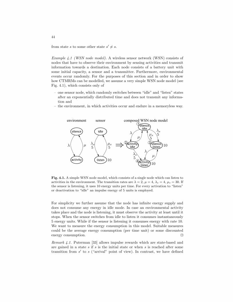
44
from state s to some other state s′ 6= s.
Example 4.1 (WSN node model). A wireless sensor network (WSN) consists ofnodes that have to observe their environment by sensing activities and transmitinformation towards a destination. Each node consists of a battery unit withsome initial capacity, a sensor and a transmitter. Furthermore, environmentalevents occur randomly. For the purposes of this section and in order to showhow CTMRMs can be modelled, we assume a very simple WSN node model (seeFig. 4.1), which consists only of
– one sensor node, which randomly switches between “idle” and “listen” statesafter an exponentially distributed time and does not transmit any informa-tion and
– the environment, in which activities occur and endure in a memoryless way.
silence
environment sensor
activity
idle
listen
silence,idle
activity,idle
composed WSN node model
activity,listen
silence,listen
1
2 3
4
Fig. 4.1. A simple WSN node model, which consists of a single node which can listen toactivities in the environment. The transition rates are λ = 2, µ = 4, λs = 4, µs = 30. Ifthe sensor is listening, it uses 10 energy units per time. For every activation to “listen”or deactivation to “idle” an impulse energy of 5 units is employed.
For simplicity we further assume that the node has infinite energy supply anddoes not consume any energy in idle mode. In case an environmental activitytakes place and the node is listening, it must observe the activity at least until itstops. When the sensor switches from idle to listen it consumes instantaneously5 energy units. While if the sensor is listening it consumes energy with rate 10.We want to measure the energy consumption in this model. Suitable measurescould be the average energy consumption (per time unit) or some discountedenergy consumption. ut
Remark 4.1. Puterman [33] allows impulse rewards which are state-based andare gained in a state s if s is the initial state or when s is reached after sometransition from s′ to s (“arrival” point of view). In contrast, we have defined
45
transition-based impulse rewards i(s, s′) that are gained when state s is left, i.e.a transition from s to s′ is performed (“departure” point of view). Therefore,the impulse reward can be considered state-based as the expectation i(s) =∑s′ 6=s i(s, s
′)P (s, s′) over transition probabilities. When considering the infinite-horizon total reward measure or the average reward measure, then both points ofview lead to the same value functions and thus their distinction doesn’t matterin this case. However, this difference is important when we are dealing with thefinite-horizon total reward measure and the discounted reward measure.
Before being able to define and evaluate reward measures for the continuous-time case, we have to provide more theoretical background. The next section isdevoted to this.
4.2 Probability Space for CTMCs
In the following, we want to formalize the transition behavior of a CTMCM =(S,Q) that we have informally introduced in Sect. 4.1. For this reason, we firstdefine a suitable sample space Ω together with a Borel σ-algebra B(Ω) consistingof those measurable events for which we will assign probabilities. Subsequently,we will define several stochastic processes upon Ω that are all induced by theCTMC M. These processes will allow us to define a time-dependent transitionprobability matrix, which in turn will play an important role for the definitionof reward measures for a CTMRM.
4.2.1 Sample SpaceSince continuous time plays a role for these measures, we put this informationalong with the state space S into the sample space. Define the sample space Ω ⊆(S× (0,∞])N as the set of infinite paths of the form ω = (s0, t0, s1, t1, s2, t2, . . . )such that for all i ∈ N:
(E(si) > 0⇒ Q(si, si+1) > 0 ∧ ti <∞) ∨ (E(si) = 0⇒ si+1 = si ∧ ti =∞) .
Roughly speaking, ω represents a sample path, where ti <∞ is the finite sojourntime in a non-absorbing state si or otherwise if si is absorbing then for all j ≥ iit holds that tj =∞ and sj = si. A sample path ω = (s0, t0, s1, t1, . . . ) can alsobe considered as a jump function ω : [0,∞) → S that is constantly s0 for allt ∈ [0, t0) and if t0 6= ∞ then ω jumps to state s1 6= s0 at t0 and ω(t) = s1
for all t ∈ [t0, t0 + t1). If t1 6= ∞ then ω has a next jump to state s2 6= s1
at t0 + t1 and so on, until there is eventually a first index i with ti = ∞ andtherefore ω(t) = si for all t ≥
∑i−1k=0 tk. In order to define a probability space
over Ω we transform Ω to the set Path of finite absorbing and infinite paths asdefined in [3]. Let ψ : Ω → Path be the transformation that drops the artificialrepetitions of absorbing states, i.e.
ψ(s0, t0, s1, t1, . . . ) :=
(s0, t0, s1, t1, . . . ), if ∀k ∈ N : tk <∞(s0, t0, s1, t1, . . . , sl), l := min k | tk =∞ <∞
46
where min ∅ := ∞. Note that in the definition of ψ the two cases are disjoint.Since ψ is bijective the probability space (Path,F(Path),Prα) as defined in [3](where α ∈ D(S) is a distribution over initial states) induces for each s ∈ S aprobability space (Ω,B(Ω), Ps) in a canonical way:
B(Ω) := A ⊆ Ω | ψ(A) ∈ F(Path) and Ps := Prδs ψ,
where we choose α := δs with δs(s′) := δs,s′ (i.e. s is the initial state). Before
moving on, we want to mention that both sample spaces Ω and Path are equiv-alent, since ψ is bijective (and measurable by definition of B(Ω)). The samplespace Path allows for an intuitive interpretation of sample paths ω regarded asjump functions ω : [0,∞)→ S as described above. Every jump function that isconstant on intervals of positive length has at most a finite or countably infinitenumber of jumps – this distinction is encoded in the sample paths of Path. How-ever, this differentiation of cases would directly be transferred to a correspondingdifferentiation in the definition of stochastic processes that we will introduce inthe sequel. For this reason, we have chosen Ω as the sample space which em-bedds these cases already in its definition and thus does not lead to an overloadof notation in the definition of these processes.
4.2.2 Induced Stochastic ProcessesThe CTMC M = (S,Q) induces a number of stochastic processes over Ω. Forω = (s0, t0, s1, t1, . . . ) ∈ Ω define the
(i) discrete-time state process (Xn)n∈N by
Xn(ω) := sn
(ii) sojourn time (τn)n∈N, where
τn(ω) := tn ≤ ∞
(iii) total elapsed time (Tn)n∈N for the first n transitions as
Tn(ω) :=
n−1∑i=0
τi(ω)
(iv) number of transitions (Nt)0≤t<∞ up to time t as
Nt(ω) := max n | Tn(ω) ≤ t ∈ N
(note that with probability 1 the maximum is taken over a finite set andthus Nt is almost surely finite, i.e. P (Nt <∞) = 1)
(v) continuous-time state process (Zt)0≤t<∞, where
Zt(ω) := XNt(ω)(ω),
i.e. Zt is the state of the system at point in time t ≥ 0.
47
Remark 4.2. For all t ∈ [0,∞) and n ∈ N the following equalities of events hold:
Nt = n = Tn ≤ t < Tn+1 and Nt ≥ n = Tn ≤ t .
The discrete-time state process Xn represents the n-th visited state (or an ab-sorbing state) and it fulfills the discrete-time Markov property as in (2.4), i.e.for all s, s0, s1, . . . sk ∈ S and 0 < n1 < · · · < nk < n
Ps0(Xn = s | Xn1= s1, . . . , Xnk = sk) = Ps0(Xn = s | Xnk = sk).
From Zt(ω) = XNt(ω)(ω) and Nt(ω) non-decreasing for all ω it follows that thecontinuous-time state process Zt also fulfills the Markov property, which readsas a continuous time version:
Ps0(Zt = s | Zt1 = s1, . . . , Ztk = sk) = Ps0(Zt = s | Ztk = sk)
for all s, s0, s1, . . . sk ∈ S and 0 ≤ t1 < · · · < tk < t. Thus given knowledgeabout the state Ztk = sk of the process for any arbitrary point in time tk < t,then the process Zt does not depend on its history comprising the visited statesbefore time tk. It further holds that Zt is homogeneous in time, i.e. the followingproperty holds:
Ps0(Zt+t′ = s′ | Zt = s) = Ps(Zt′ = s′).
As in Sect. 2 we fix a representation of the state space S through indices1, 2, . . . , n , n := |S| such that functions S → R can be represented by vec-tors in Rn and functions S × S → R as matrices in Rn×n. Define the transientprobability matrix P (t) as
P (t)(s, s′) := Ps(Zt = s′). (4.1)
The matrix P (t) is stochastic for all t ≥ 0 and fulfills the property
P (t+ t′) = P (t)P (t′) ∀t, t′ ≥ 0,
which reads componentwise as P (t+ t′)(s, s′) =∑u P (t)(s, u) ·P (t′)(u, s′). This
means that from state s the probability to be in state s′ after t+ t′ time units isthe probability to be in some arbitrary state u ∈ S after t time units and traversefrom there within further t′ time units to state s′. It can be shown that all entriesof P (t) are differentiable for all t ≥ 0 and P (t) is related to the generator matrixQ of the CTMC by the Kolmogorov differential equations
d
dtP (t) = QP (t) and
d
dtP (t) = P (t)Q, (4.2)
which read in componentwise notation as
d
dt(P (t)(s, s′)) =
∑u
Q(s, u) · P (t)(u, s′) =∑v
P (t)(s, v) ·Q(v, s′).
All solutions to these equations are of the form P (t) = eQt since P (0) = I isthe identity matrix, where for a matrix A the quantity eA denotes the matrixexponential that is given by eA =
∑∞k=0
1k!A
k.
48
4.2.3 State ClassificationAs in Sect. 2.1.2 there is also a classification of states in case of continuous timeMarkov chains. Since this taxonomy is almost the same as in the discrete-timecase, we only present it very briefly. The most important difference is that inthe continuous-time setup there is no notion for periodicity of states and it canbe shown that the matrix P (t) converges as t→∞ (for finite state spaces). Wedenote the limit by P ∗ := limt→∞ P (t). Note that in Definition 2.9 we denotedthe corresponding discrete-time limiting matrix as P∞ and its time-averagedversion as P ∗ and mentioned in Proposition 2.2 that they both coincide if P∞
exists. Since the existence of this limit in the continuous-time case is alwaysguaranteed, we call this limit directly P ∗ instead of P∞ in order to use similarnotation. One can show that P ∗ is stochastic and fulfills the invariance conditions
P ∗P (t) = P (t)P ∗ = P ∗P ∗ = P ∗.
Therefore, the probability distribution P ∗(s, ·) ∈ D(S) in each row of P ∗ is astationary distribution and since P (t)(s, ·)→ P ∗(s, ·) as t→∞ it is also thelimiting distribution from state s. Furthermore, it holds that
P ∗Q = QP ∗ = 0,
which can be derived from (4.2) and ddtP (t)→ 0 as t→∞.
Let the random variable Ms ∈ (0,∞] denote the point in time when the stateprocess Zt returns to s for the first time (given Z0 = s). A state s is tran-sient if Ps(Ms = ∞) > 0 or equivalently P ∗(s, s) = 0. In the other case,if Ps(Ms <∞) = 1 then s is called recurrent and it holds equivalently thatP ∗(s, s) > 0. It can be shown that there is always at least one recurrent stateif the state space is finite. A state s′ is reachable from s if P (t)(s, s′) > 0 forsome t ≥ 0. The states s and s′ are communicating if s′ is reachable from sand s is reachable from s′. This communication relation is an equivalence rela-tion and partitions the set of recurrent states into closed recurrent classes.Therefore, the state space partitions into S =
⋃ki=1 S
ri ∪ St, where St denotes
the set of transient states and Sri is a closed recurrent class for all i = 1, . . . , k.For s, s′ ∈ Sri in the same recurrent class it holds that P ∗(s, s′) > 0. As in thediscrete-time case P ∗ can be represented by
P ∗ =
P ∗1 0 0 . . . 0 00 P ∗2 0 . . . 0 0...
......
. . .... 0
0 0 0 . . . P ∗k 0
P ∗1 P ∗2 P ∗3 . . . P ∗k 0
(4.3)
where P ∗i has identical rows for the stationary distribution in class Sri and P ∗icontains the trapping probabilities from transient states St into Sri . If a closedrecurrent class consists of only one state s, then s is called absorbing. A CTMCis unichain if k = 1 and multichain if k ≥ 2. A unichain CTMC is calledirreducible or ergodic if St = ∅.
49
4.3 Model Transformations
In this section we present a set of model transformations, which will allow us to
– unify the different types of rewards (impulse reward and rate reward) in thereward accumulation process (“Continuization”) and
– relate some continuous-time concepts to discrete-time Markov Reward Mod-els from Sect. 2 (“Embedding” and “Uniformization”).
These transformations simplify the evaluation process of all the reward measuresand map the computation of the value functions for continuous-time models tothe discrete-time case.
4.3.1 EmbeddingAs mentioned in Sect. 4.1, a CTMC (S,Q) defines for all states s, s′ ∈ S theembedded transition probabilities P (s, s′). The structure (S, P ) can be con-sidered as a discrete-time Markov chain and it induces on the sample spaceΩ′ :=
(s0, s1, s2, . . . ) ∈ SN | P (si−1, si) > 0 for all i ≥ 1
as in (2.3) the state
process X ′n (by Definition 2.3) given by X ′n(s0, s1, . . . ) = sn. This stochasticprocess is related to the discrete-time state process Xn : Ω → S by abstractingaway from the time information, i.e. for all n ∈ N
Xn(s0, t0, s1, t1, . . . ) = X ′n(s0, s1, . . . ).
This equation establishes the connection to DTMCs and thus Xn can be con-sidered as the state process of the DTMC (S, P ). Therefore, (S, P ) is also calledthe embedded discrete-time Markov chain and Xn is the embedded stateprocess of the CTMC (S,Q).Now consider a CTMRM (S,Q, i, r) and define a function R : S × S → R whereR(s, s′) denotes the expected accumulated rate reward r(s) in state s over timeincluding the impulse reward i(s, s′) gained for transition from s to some otherstate s′ 6= s (as in Sect. 4.1). If s is non-absorbing, then the sojourn time τs ins is exponentially distributed with rate E(s) > 0 and R(s, s′) is given by
R(s, s′) := i(s, s′) +r(s)
E(s). (4.4)
Otherwise, if s is absorbing, the embedding is only possible if r(s) = 0 and inthis case we define R(s, s′) := 0 for all s′.It is very important to note that if we consider a reward measure on the CTMRMwith value function V and a corresponding reward measure on the transformedDTMRM with value function V ′, then it is of course desirable that V = V ′, i.e.the transformation should be value-preserving. This allows to compute thevalue V by applying the theory and algorithms for the discrete-time models aspresented in Sect. 2. However, as we will see, such a model transformation needsin general the reward measure itself as input in order to be value-preserving.As an example, the integration of the rate reward r(s) into the reward R(s, s′)
50
is performed by total expectation over an infinite time-horizon, which gives the
term r(s)E(s) . If one considers a finite horizon for the continuous-time model, then
R(s, s′) as defined is obviously not the appropriate reward gained in state s inthe embedded discrete-time model.
4.3.2 UniformizationWe have seen in Sect. 4.1 that the quantities Q(s, s′) for s′ 6= s can be re-garded as rates of exponentially distributed transition times τs,s′ . All thesetransition events define a race and only the fastest event involves a transi-tion to another state s′ 6= s. We can manipulate this race, by adding to theset of events τs,s′ | s′ 6= s of a state s an auxiliary exponentially distributedevent τs,s with an arbitrary positive rate L(s) > 0 that introduces a self-loop(i.e. a transition from s to s), if it wins the race. The time up to transition isτs := min τs,s′ | s′ ∈ S and it is exponentially distributed with increased exit
rate E(s) := E(s) + L(s). The probability that τs,s wins the race can be com-
puted to P (τs,s ≤ τs,s′ ∀s′ ∈ S) = L(s)
E(s)= 1 + Q(s,s)
E(s)and for all s′0 6= s it holds
that P (τs,s′0 ≤ τs,s′ ∀s′ ∈ S) = Q(s,s′)
E(s). We can add such events τs,s to a set
of states s and thus increase the exit rates for all these states simultaneously.Moreover, we can choose an arbitrary µ > 0 with max E(s) | s ∈ S ≤ µ < ∞(called uniformization rate) such that E(s) ≡ µ is constant for all s ∈ S. Theuniformization rate µ allows to define a transformation to the µ-uniformizedDTMRM Mµ := (S, Pµ, Rµ) where a transition from s to s′ in Mµ capturesthe event that τs,s′ wins the race and thus
Pµ(s, s′) := δs,s′ +Q(s, s′)
µ. (4.5)
Note that the probability to eventually leave state s to a state s′ 6= s is exactlythe embedded transition probability P (s, s′) =
∑∞i=0 P
µ(s, s)iPµ(s, s′). The re-ward Rµ(s, s′) combines the accumulated rate reward in state s and the impulsereward up to transition to some state s′. In the CTMRM the rate reward r(s)is accumulated for the complete sojourn time in s. Since self-loops are possiblein the uniformized DTMRM the accumulation process stops when an arbitrarytransition occurs. The expected value of the accumulated rate reward up to tran-sition is given by r(s) · 1
µ . Furthermore, the impulse reward i(s, s′) is only gained
if a transition to another state s′ 6= s takes place. But since i(s, s) = 0 for alls ∈ S by Definition 4.1 it follows that for all s, s′ ∈ S the total uniformizedreward Rµ(s, s′) is given by
Rµ(s, s′) := i(s, s′) +r(s)
µ. (4.6)
This equation is similar to (4.4) with the difference that the exit rate E(s) isreplaced by the uniformization rate µ ≥ E(s). A further difference comes intothe picture when considering the accumulation of these rewards. Both rewards
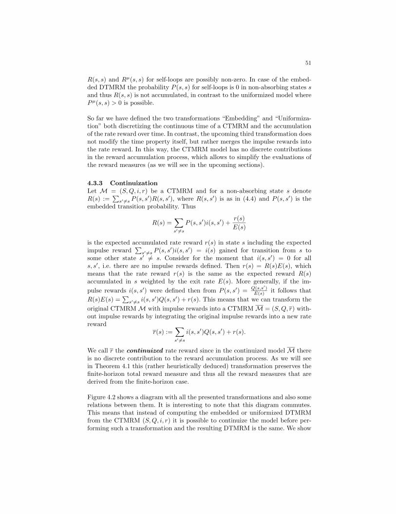
51
R(s, s) and Rµ(s, s) for self-loops are possibly non-zero. In case of the embed-ded DTMRM the probability P (s, s) for self-loops is 0 in non-absorbing states sand thus R(s, s) is not accumulated, in contrast to the uniformized model wherePµ(s, s) > 0 is possible.
So far we have defined the two transformations “Embedding” and “Uniformiza-tion” both discretizing the continuous time of a CTMRM and the accumulationof the rate reward over time. In contrast, the upcoming third transformation doesnot modify the time property itself, but rather merges the impulse rewards intothe rate reward. In this way, the CTMRM model has no discrete contributionsin the reward accumulation process, which allows to simplify the evaluations ofthe reward measures (as we will see in the upcoming sections).
4.3.3 ContinuizationLet M = (S,Q, i, r) be a CTMRM and for a non-absorbing state s denoteR(s) :=
∑s′ 6=s P (s, s′)R(s, s′), where R(s, s′) is as in (4.4) and P (s, s′) is the
embedded transition probability. Thus
R(s) =∑s′ 6=s
P (s, s′)i(s, s′) +r(s)
E(s)
is the expected accumulated rate reward r(s) in state s including the expectedimpulse reward
∑s′ 6=s P (s, s′)i(s, s′) = i(s) gained for transition from s to
some other state s′ 6= s. Consider for the moment that i(s, s′) = 0 for alls, s′, i.e. there are no impulse rewards defined. Then r(s) = R(s)E(s), whichmeans that the rate reward r(s) is the same as the expected reward R(s)accumulated in s weighted by the exit rate E(s). More generally, if the im-
pulse rewards i(s, s′) were defined then from P (s, s′) = Q(s,s′)E(s) it follows that
R(s)E(s) =∑s′ 6=s i(s, s
′)Q(s, s′) + r(s). This means that we can transform the
original CTMRMM with impulse rewards into a CTMRMM = (S,Q, r) with-out impulse rewards by integrating the original impulse rewards into a new ratereward
r(s) :=∑s′ 6=s
i(s, s′)Q(s, s′) + r(s).
We call r the continuized rate reward since in the continuized model M thereis no discrete contribution to the reward accumulation process. As we will seein Theorem 4.1 this (rather heuristically deduced) transformation preserves thefinite-horizon total reward measure and thus all the reward measures that arederived from the finite-horizon case.
Figure 4.2 shows a diagram with all the presented transformations and also somerelations between them. It is interesting to note that this diagram commutes.This means that instead of computing the embedded or uniformized DTMRMfrom the CTMRM (S,Q, i, r) it is possible to continuize the model before per-forming such a transformation and the resulting DTMRM is the same. We show
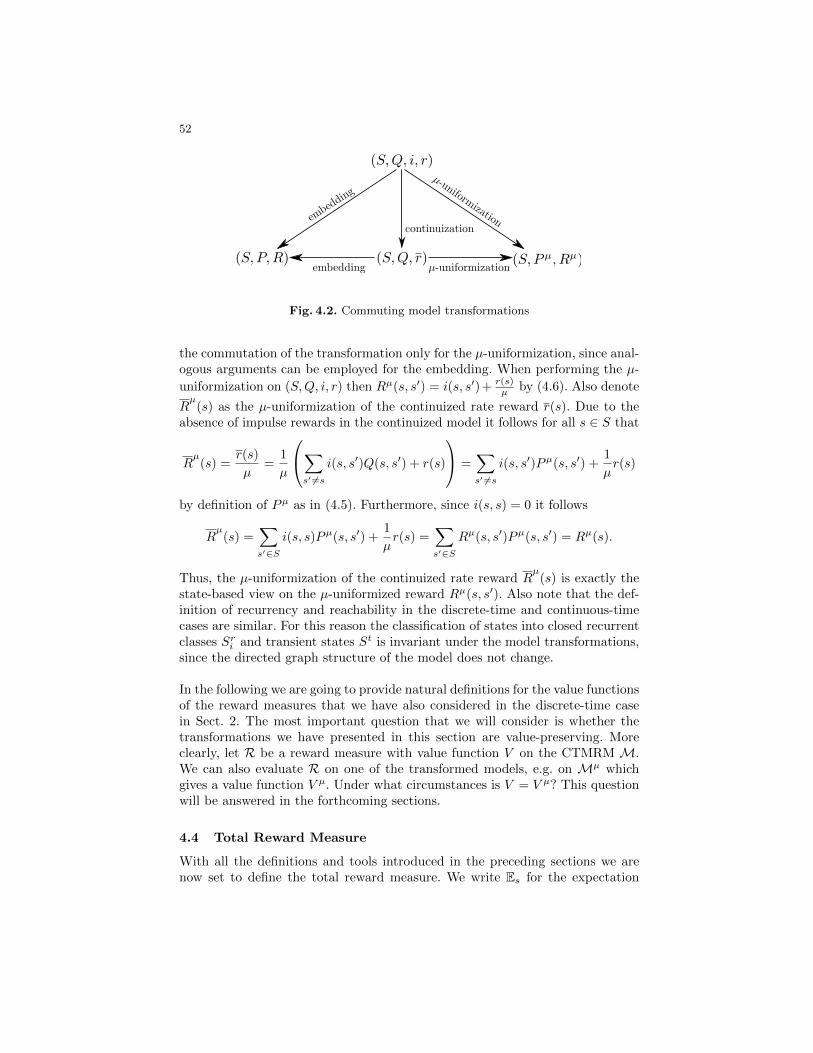
52
Fig. 4.2. Commuting model transformations
the commutation of the transformation only for the µ-uniformization, since anal-ogous arguments can be employed for the embedding. When performing the µ-
uniformization on (S,Q, i, r) then Rµ(s, s′) = i(s, s′)+ r(s)µ by (4.6). Also denote
Rµ(s) as the µ-uniformization of the continuized rate reward r(s). Due to the
absence of impulse rewards in the continuized model it follows for all s ∈ S that
Rµ(s) =
r(s)
µ=
1
µ
∑s′ 6=s
i(s, s′)Q(s, s′) + r(s)
=∑s′ 6=s
i(s, s′)Pµ(s, s′) +1
µr(s)
by definition of Pµ as in (4.5). Furthermore, since i(s, s) = 0 it follows
Rµ(s) =
∑s′∈S
i(s, s)Pµ(s, s′) +1
µr(s) =
∑s′∈S
Rµ(s, s′)Pµ(s, s′) = Rµ(s).
Thus, the µ-uniformization of the continuized rate reward Rµ(s) is exactly the
state-based view on the µ-uniformized reward Rµ(s, s′). Also note that the def-inition of recurrency and reachability in the discrete-time and continuous-timecases are similar. For this reason the classification of states into closed recurrentclasses Sri and transient states St is invariant under the model transformations,since the directed graph structure of the model does not change.
In the following we are going to provide natural definitions for the value functionsof the reward measures that we have also considered in the discrete-time casein Sect. 2. The most important question that we will consider is whether thetransformations we have presented in this section are value-preserving. Moreclearly, let R be a reward measure with value function V on the CTMRM M.We can also evaluate R on one of the transformed models, e.g. on Mµ whichgives a value function V µ. Under what circumstances is V = V µ? This questionwill be answered in the forthcoming sections.
4.4 Total Reward Measure
With all the definitions and tools introduced in the preceding sections we arenow set to define the total reward measure. We write Es for the expectation
53
operator if X0 = s (or Z0 = s) is the initial state. For a random variable Y wealso write E[Y ] for the function s 7→ Es [Y ] ∈ R, respectively for the vector inR|S| consisting of the expected values Es[Y ].
Definition 4.2. Let T ∈ R, T ≥ 0 be some finite real time horizon and NT therandom number of transitions up to time T . The finite-horizon total valuefunction is defined as
VT (s) := Es
[NT∑k=1
i(Xk−1, Xk)
]+ Es
[∫ T
0
r(Zt) dt
], (4.7)
if both expectations exist. If furthermore the expectations Es[∑NT
k=1 |i(Xk−1, Xk)|]
and Es[∫ T
0|r(Zt)| dt
]converge as T → ∞, then we also define the (infinite-
horizon) total value function as
V∞(s) := limT→∞
VT (s).
In (4.7) the rate reward r(Zt) in state Zt is continuously accumulated over thetime interval [0, T ] by integration, whereas the impulse rewards i(Xk−1, Xk) forthe NT transitions from states Xk−1 to Xk for k = 1, . . . , NT are discretely ac-cumulated via summation. Note that the upper bound NT = max n | Tn ≤ Tin the summation is random. If ω = (s0, t0, s1, t1, . . . ) ∈ Ω then NT (ω) ∈ N and
the random variable∑NTk=1 i(Xk−1, Xk) takes the value
∑NT (ω)k=1 i(sk−1, sk) ∈ R.
Furthermore, NT has finite expectation (see Lemma 7.3 in the Appendix). Sincethe state space is finite there exists C ≥ 0 such that |r(s)| ≤ C and |i(s, s′)| ≤ Cfor all s, s′ ∈ S. Therefore
Es
[∣∣∣∣∣∫ T
0
r(Zt) dt
∣∣∣∣∣]≤ C ·T <∞ and Es
[∣∣∣∣∣NT∑k=1
i(Xk−1, Xk)
∣∣∣∣∣]≤ C ·E [NT ] <∞
such that VT (s) is defined for all T ≥ 0. In the prerequisites for the definition ofthe total value function V∞ we require a more restrictive absolute convergence.However, this property is quite natural since it is equivalent to the (joint) inte-grability of the function r(Zt) : [0,∞)×Ω → R with respect to the probabilitymeasure Ps on Ω for the expectation Es and the Lebesgue measure for the inte-gral over [0,∞).Note that Es [r(Zt)] =
∑s′ Ps(Zt = s′)r(s′) is the s-th row of the vector P (t)r.
If we assume that i(s, s′) = 0 for all s, s′ ∈ S then the finite-horizon total valuefunction VT ∈ RS regarded as a vector in R|S| can be computed by
VT = E
[∫ T
0
r(Zt) dt
]=
∫ T
0
P (t)r dt. (4.8)
The following theorem generalizes this computation for the case with impulserewards i(s, s′). Furthermore, it explains why the continuization transformationas defined in Sect. 4.3.3 preserves the finite-horizon total reward measure. There-fore, this can be considered as the main theorem in the section on CTMRMs.
54
Theorem 4.1 (Value Preservation of Continuization).For a CTMRM M = (S,Q, i, r) let M = (S,Q, r) be its continuization with
r(s) =∑s′ 6=s
i(s, s′)Q(s, s′) + r(s).
For the finite-horizon total value function it holds that
VT (s) = Es
[∫ T
0
r(Zt) dt
].
VT can be computed by
VT =
∫ T
0
P (t)r dt,
which reads in componentwise notation as
VT (s) =∑s′∈S
r(s′)
∫ T
0
P (t)(s, s′) dt.
Proof. In (4.8) we have already shown the statement for the integral term in thedefinition of VT in (4.7). It remains to show the statement for the summationterm. We have already mentioned that NT has finite expectation. By Lemma7.1 in the Appendix and the law of total expectation it follows for an arbitraryinitial state s0 ∈ S that
Es0
[NT∑k=1
i(Xk−1, Xk)
]=
∞∑k=1
Es0 [i(Xk−1, Xk)]Ps0(NT ≥ k) =
∞∑k=1
∑s,s′
i(s, s′)Ps0(Xk−1 = s,Xk = s′)Ps0(NT ≥ k) =∑s,s′
i(s, s′)nT (s, s′),
where
nT (s, s′) :=Es0
[NT∑k=1
1Xk−1=s,Xk=s′
]=
∞∑k=1
Ps0(Xk−1 = s,Xk = s′)Ps0(NT ≥ k)
is the expected number of transitions from s to s′ up to time T from initial states0. If we can show that
nT (s, s′) = Q(s, s′) ·∫ T
0
Ps0(Zt = s) dt
then we are done. The proof for this equation is outsourced to the Appendix.There, in Lemma 7.2 we present a proof which uses the uniformization methodand in Remark 7.2 we sketch a more direct proof without the detour with uni-formization which relies on facts from queueing theory. ut
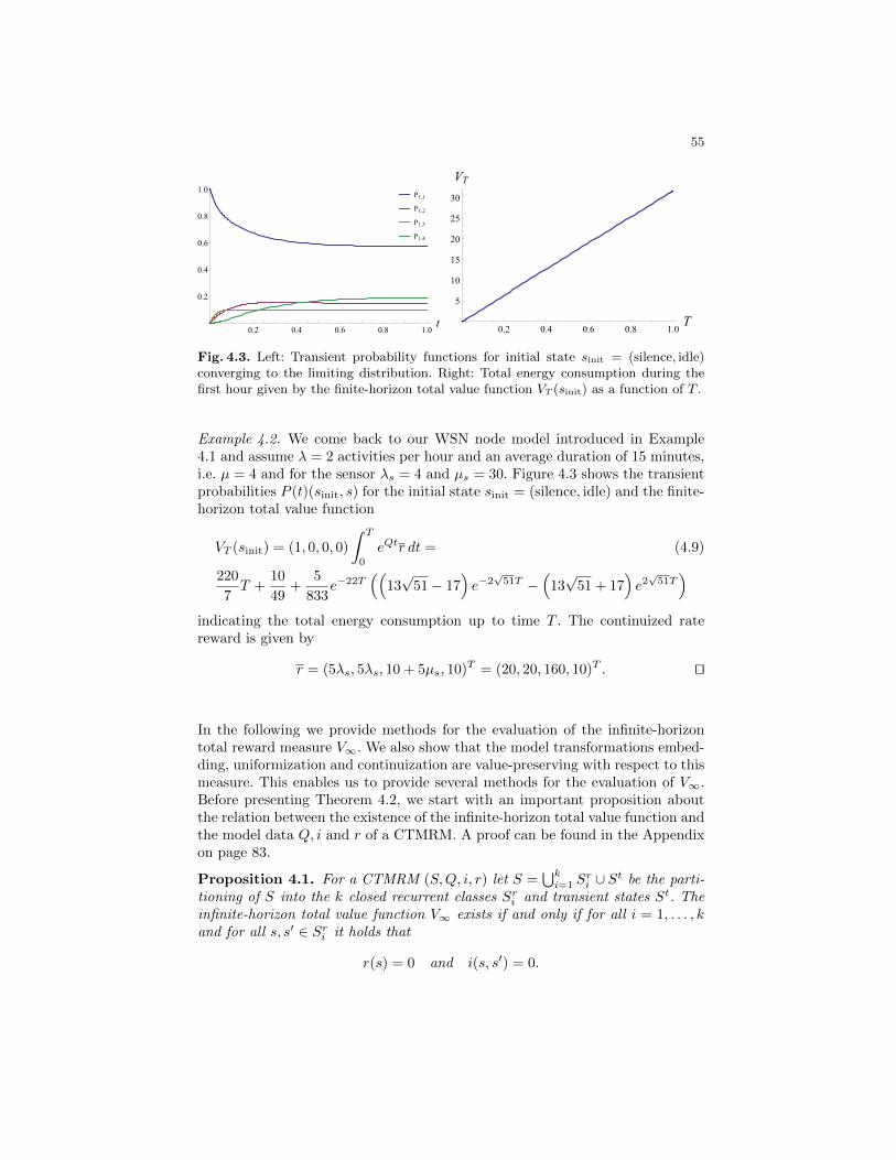
55
P1,1
P1,2
P1,3
P1,4
0.2 0.4 0.6 0.8 1.0t
0.2
0.4
0.6
0.8
1.0
0.2 0.4 0.6 0.8 1.0T
5
10
15
20
25
30
VT
Fig. 4.3. Left: Transient probability functions for initial state sinit = (silence, idle)converging to the limiting distribution. Right: Total energy consumption during thefirst hour given by the finite-horizon total value function VT (sinit) as a function of T .
Example 4.2. We come back to our WSN node model introduced in Example4.1 and assume λ = 2 activities per hour and an average duration of 15 minutes,i.e. µ = 4 and for the sensor λs = 4 and µs = 30. Figure 4.3 shows the transientprobabilities P (t)(sinit, s) for the initial state sinit = (silence, idle) and the finite-horizon total value function
VT (sinit) = (1, 0, 0, 0)
∫ T
0
eQtr dt = (4.9)
220
7T +
10
49+
5
833e−22T
((13√
51− 17)e−2√
51T −(
13√
51 + 17)e2√
51T)
indicating the total energy consumption up to time T . The continuized ratereward is given by
r = (5λs, 5λs, 10 + 5µs, 10)T = (20, 20, 160, 10)T . ut
In the following we provide methods for the evaluation of the infinite-horizontotal reward measure V∞. We also show that the model transformations embed-ding, uniformization and continuization are value-preserving with respect to thismeasure. This enables us to provide several methods for the evaluation of V∞.Before presenting Theorem 4.2, we start with an important proposition aboutthe relation between the existence of the infinite-horizon total value function andthe model data Q, i and r of a CTMRM. A proof can be found in the Appendixon page 83.
Proposition 4.1. For a CTMRM (S,Q, i, r) let S =⋃ki=1 S
ri ∪ St be the parti-
tioning of S into the k closed recurrent classes Sri and transient states St. Theinfinite-horizon total value function V∞ exists if and only if for all i = 1, . . . , kand for all s, s′ ∈ Sri it holds that
r(s) = 0 and i(s, s′) = 0.
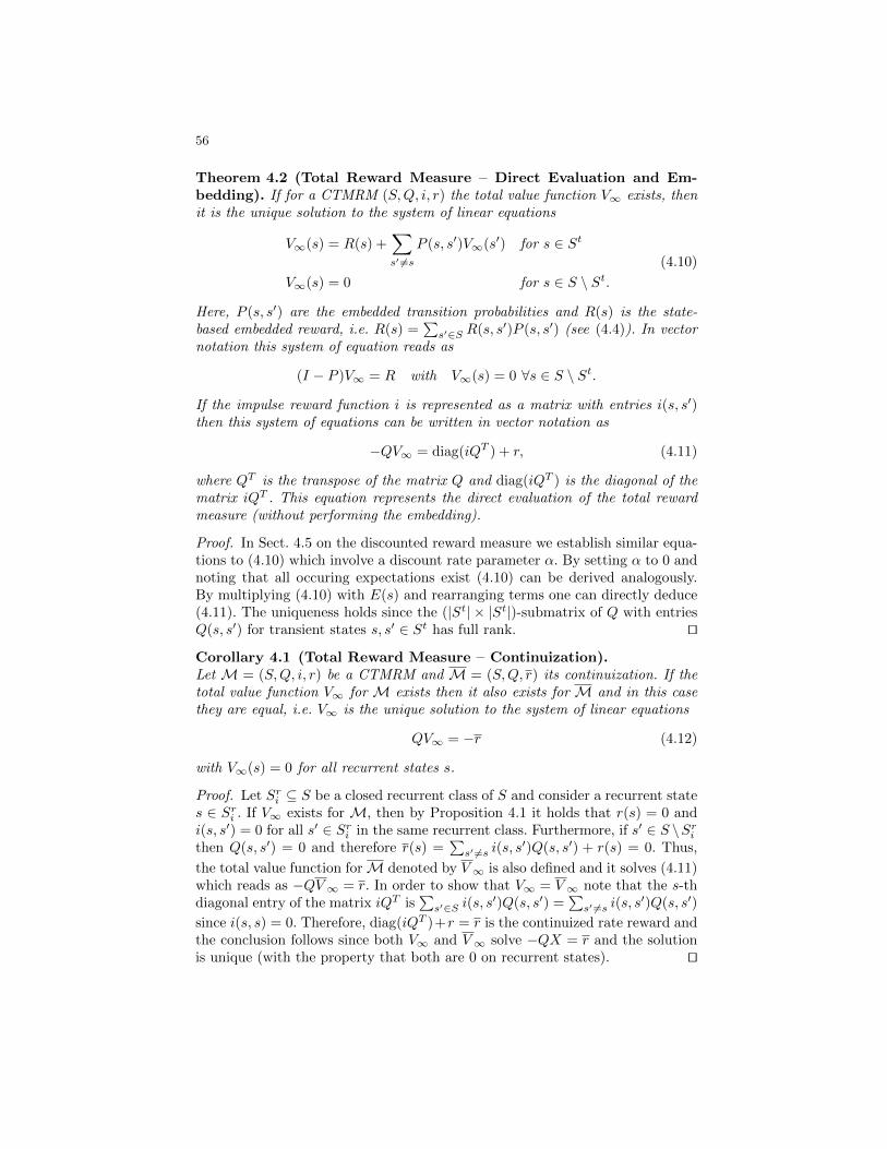
56
Theorem 4.2 (Total Reward Measure – Direct Evaluation and Em-bedding). If for a CTMRM (S,Q, i, r) the total value function V∞ exists, thenit is the unique solution to the system of linear equations
V∞(s) = R(s) +∑s′ 6=s
P (s, s′)V∞(s′) for s ∈ St
V∞(s) = 0 for s ∈ S \ St.(4.10)
Here, P (s, s′) are the embedded transition probabilities and R(s) is the state-based embedded reward, i.e. R(s) =
∑s′∈S R(s, s′)P (s, s′) (see (4.4)). In vector
notation this system of equation reads as
(I − P )V∞ = R with V∞(s) = 0 ∀s ∈ S \ St.
If the impulse reward function i is represented as a matrix with entries i(s, s′)then this system of equations can be written in vector notation as
−QV∞ = diag(iQT ) + r, (4.11)
where QT is the transpose of the matrix Q and diag(iQT ) is the diagonal of thematrix iQT . This equation represents the direct evaluation of the total rewardmeasure (without performing the embedding).
Proof. In Sect. 4.5 on the discounted reward measure we establish similar equa-tions to (4.10) which involve a discount rate parameter α. By setting α to 0 andnoting that all occuring expectations exist (4.10) can be derived analogously.By multiplying (4.10) with E(s) and rearranging terms one can directly deduce(4.11). The uniqueness holds since the (|St| × |St|)-submatrix of Q with entriesQ(s, s′) for transient states s, s′ ∈ St has full rank. ut
Corollary 4.1 (Total Reward Measure – Continuization).Let M = (S,Q, i, r) be a CTMRM and M = (S,Q, r) its continuization. If thetotal value function V∞ for M exists then it also exists for M and in this casethey are equal, i.e. V∞ is the unique solution to the system of linear equations
QV∞ = −r (4.12)
with V∞(s) = 0 for all recurrent states s.
Proof. Let Sri ⊆ S be a closed recurrent class of S and consider a recurrent states ∈ Sri . If V∞ exists for M, then by Proposition 4.1 it holds that r(s) = 0 andi(s, s′) = 0 for all s′ ∈ Sri in the same recurrent class. Furthermore, if s′ ∈ S \Srithen Q(s, s′) = 0 and therefore r(s) =
∑s′ 6=s i(s, s
′)Q(s, s′) + r(s) = 0. Thus,
the total value function forM denoted by V∞ is also defined and it solves (4.11)which reads as −QV∞ = r. In order to show that V∞ = V∞ note that the s-thdiagonal entry of the matrix iQT is
∑s′∈S i(s, s
′)Q(s, s′) =∑s′ 6=s i(s, s
′)Q(s, s′)
since i(s, s) = 0. Therefore, diag(iQT )+r = r is the continuized rate reward andthe conclusion follows since both V∞ and V∞ solve −QX = r and the solutionis unique (with the property that both are 0 on recurrent states). ut
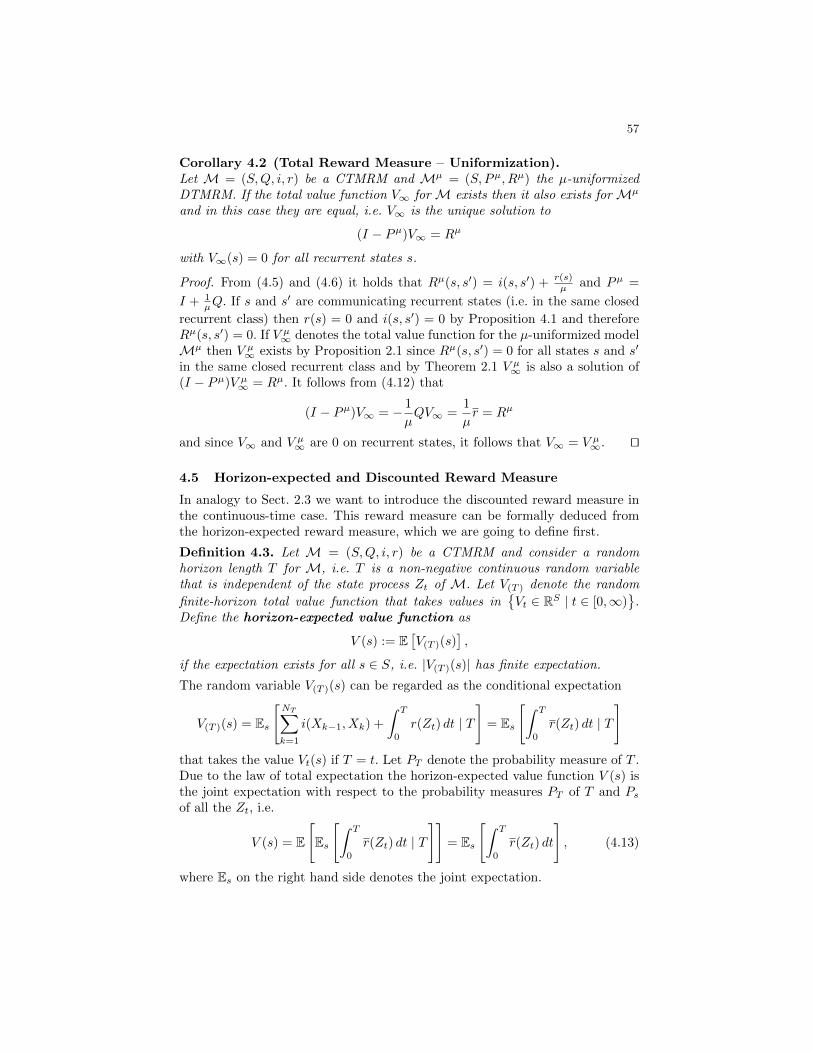
57
Corollary 4.2 (Total Reward Measure – Uniformization).Let M = (S,Q, i, r) be a CTMRM and Mµ = (S, Pµ, Rµ) the µ-uniformizedDTMRM. If the total value function V∞ for M exists then it also exists for Mµ
and in this case they are equal, i.e. V∞ is the unique solution to
(I − Pµ)V∞ = Rµ
with V∞(s) = 0 for all recurrent states s.
Proof. From (4.5) and (4.6) it holds that Rµ(s, s′) = i(s, s′) + r(s)µ and Pµ =
I + 1µQ. If s and s′ are communicating recurrent states (i.e. in the same closed
recurrent class) then r(s) = 0 and i(s, s′) = 0 by Proposition 4.1 and thereforeRµ(s, s′) = 0. If V µ∞ denotes the total value function for the µ-uniformized modelMµ then V µ∞ exists by Proposition 2.1 since Rµ(s, s′) = 0 for all states s and s′
in the same closed recurrent class and by Theorem 2.1 V µ∞ is also a solution of(I − Pµ)V µ∞ = Rµ. It follows from (4.12) that
(I − Pµ)V∞ = − 1
µQV∞ =
1
µr = Rµ
and since V∞ and V µ∞ are 0 on recurrent states, it follows that V∞ = V µ∞. ut
4.5 Horizon-expected and Discounted Reward Measure
In analogy to Sect. 2.3 we want to introduce the discounted reward measure inthe continuous-time case. This reward measure can be formally deduced fromthe horizon-expected reward measure, which we are going to define first.
Definition 4.3. Let M = (S,Q, i, r) be a CTMRM and consider a randomhorizon length T for M, i.e. T is a non-negative continuous random variablethat is independent of the state process Zt of M. Let V(T ) denote the random
finite-horizon total value function that takes values inVt ∈ RS | t ∈ [0,∞)
.
Define the horizon-expected value function as
V (s) := E[V(T )(s)
],
if the expectation exists for all s ∈ S, i.e. |V(T )(s)| has finite expectation.
The random variable V(T )(s) can be regarded as the conditional expectation
V(T )(s) = Es
[NT∑k=1
i(Xk−1, Xk) +
∫ T
0
r(Zt) dt | T
]= Es
[∫ T
0
r(Zt) dt | T
]that takes the value Vt(s) if T = t. Let PT denote the probability measure of T .Due to the law of total expectation the horizon-expected value function V (s) isthe joint expectation with respect to the probability measures PT of T and Psof all the Zt, i.e.
V (s) = E
[Es
[∫ T
0
r(Zt) dt | T
]]= Es
[∫ T
0
r(Zt) dt
], (4.13)
where Es on the right hand side denotes the joint expectation.
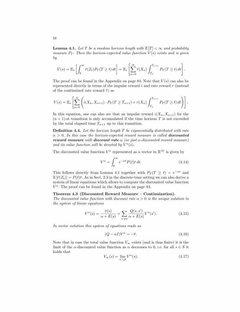
58
Lemma 4.1. Let T be a random horizon length with E [T ] <∞ and probabilitymeasure PT . Then the horizon-expected value function V (s) exists and is givenby
V (s) = Es[∫ ∞
0
r(Zt)PT (T ≥ t) dt]
= Es
[ ∞∑n=0
r(Xn)
∫ Tn+1
Tn
PT (T ≥ t) dt
].
The proof can be found in the Appendix on page 84. Note that V (s) can also berepresented directly in terms of the impulse reward i and rate reward r (insteadof the continuized rate reward r) as
V (s) = Es
[ ∞∑n=0
(i(Xn, Xn+1) · PT (T ≥ Tn+1) + r(Xn)
∫ Tn+1
Tn
PT (T ≥ t) dt
)].
In this equation, one can also see that an impulse reward i(Xn, Xn+1) for the(n + 1)-st transition is only accumulated if the time horizon T is not exceededby the total elapsed time Tn+1 up to this transition.
Definition 4.4. Let the horizon length T be exponentially distributed with rateα > 0. In this case the horizon-expected reward measure is called discountedreward measure with discount rate α (or just α-discounted reward measure)and its value function will be denoted by V α(s).
The discounted value function V α represented as a vector in R|S| is given by
V α =
∫ ∞0
e−αtP (t)r dt. (4.14)
This follows directly from Lemma 4.1 together with PT (T ≥ t) = e−αt andE [r(Zt)] = P (t)r. As in Sect. 2.3 in the discrete-time setting we can also derive asystem of linear equations which allows to compute the discounted value functionV α. The proof can be found in the Appendix on page 84.
Theorem 4.3 (Discounted Reward Measure – Continuization).The discounted value function with discount rate α > 0 is the unique solution tothe system of linear equations
V α(s) =r(s)
α+ E(s)+∑s′ 6=s
Q(s, s′)
α+ E(s)V α(s′). (4.15)
In vector notation this system of equations reads as
(Q− αI)V α = −r. (4.16)
Note that in case the total value function V∞ exists (and is thus finite) it is thelimit of the α-discounted value function as α decreases to 0, i.e. for all s ∈ S itholds that
V∞(s) = limα0
V α(s). (4.17)
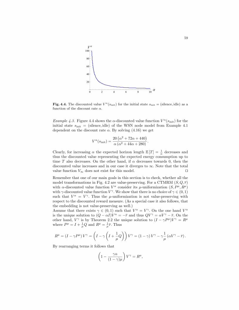
59
0 2 4 6 8 10Α
20
40
60
80
100V
Α
Fig. 4.4. The discounted value V α(sinit) for the initial state sinit = (silence, idle) as afunction of the discount rate α.
Example 4.3. Figure 4.4 shows the α-discounted value function V α(sinit) for theinitial state sinit = (silence, idle) of the WSN node model from Example 4.1dependent on the discount rate α. By solving (4.16) we get
V α(sinit) =20(α2 + 72α+ 440
)α (α2 + 44α+ 280)
.
Clearly, for increasing α the expected horizon length E [T ] = 1α decreases and
thus the discounted value representing the expected energy consumption up totime T also decreases. On the other hand, if α decreases towards 0, then thediscounted value increases and in our case it diverges to ∞. Note that the totalvalue function V∞ does not exist for this model. ut
Remember that one of our main goals in this section is to check, whether all themodel transformations in Fig. 4.2 are value-preserving. For a CTMRM (S,Q, r)with α-discounted value function V α consider its µ-uniformization (S, Pµ, Rµ)with γ-discounted value function V γ . We show that there is no choice of γ ∈ (0, 1)such that V α = V γ . Thus the µ-uniformization is not value-preserving withrespect to the discounted reward measure. (As a special case it also follows, thatthe embedding is not value-preserving as well.)Assume that there exists γ ∈ (0, 1) such that V α = V γ . On the one hand V α
is the unique solution to (Q − αI)V α = −r and thus QV γ = αV γ − r. On theother hand, V γ is by Theorem 2.2 the unique solution to (I − γPµ)V γ = Rµ
where Pµ = I + 1µQ and Rµ = 1
µr. Thus
Rµ = (I − γPµ)V γ =
(I − γ
(I +
1
µQ
))V γ = (1− γ)V γ − γ 1
µ(αV γ − r) .
By rearranging terms it follows that(1− γα
(1− γ)µ
)V γ = Rµ,
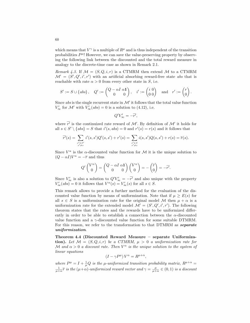
60
which means that V γ is a multiple of Rµ and is thus independent of the transitionprobabilities Pµ! However, we can save the value-preserving property by observ-ing the following link between the discounted and the total reward measure inanalogy to the discrete-time case as shown in Remark 2.1.
Remark 4.3. If M = (S,Q, i, r) is a CTMRM then extend M to a CTMRMM′ = (S′, Q′, i′, r′) with an artificial absorbing reward-free state abs that isreachable with rate α > 0 from every other state in S, i.e.
S′ := S ∪ abs , Q′ :=
(Q− αI α1
0 0
), i′ :=
(i 00 0
)and r′ :=
(r0
).
Since abs is the single recurrent state inM′ it follows that the total value functionV ′∞ for M′ with V ′∞(abs) = 0 is a solution to (4.12), i.e.
Q′V ′∞ = −r′,
where r′ is the continuized rate reward of M′. By definition of M′ it holds forall s ∈ S′ \ abs = S that i′(s, abs) = 0 and r′(s) = r(s) and it follows that
r′(s) =∑s′∈S′s′ 6=s
i′(s, s′)Q′(s, s′) + r′(s) =∑s′∈Ss′ 6=s
i(s, s′)Q(s, s′) + r(s) = r(s).
Since V α is the α-discounted value function for M it is the unique solution to(Q− αI)V α = −r and thus
Q′(V α
0
)=
(Q− αI α1
0 0
)(V α
0
)= −
(r0
)= −r′.
Since V ′∞ is also a solution to Q′V ′∞ = −r′ and also unique with the propertyV ′∞(abs) = 0 it follows that V α(s) = V ′∞(s) for all s ∈ S.
This remark allows to provide a further method for the evaluation of the dis-counted value function by means of uniformization. Note that if µ ≥ E(s) forall s ∈ S is a uniformization rate for the original model M then µ + α is auniformization rate for the extended model M′ = (S′, Q′, i′, r′). The followingtheorem states that the rates and the rewards have to be uniformized differ-ently in order to be able to establish a connection between the α-discountedvalue function and a γ-discounted value function for some suitable DTMRM.For this reason, we refer to the transformation to that DTMRM as separateuniformization.
Theorem 4.4 (Discounted Reward Measure – separate Uniformiza-tion). Let M = (S,Q, i, r) be a CTMRM, µ > 0 a uniformization rate forM and α > 0 a discount rate. Then V α is the unique solution to the system oflinear equations
(I − γPµ)V α = Rµ+α,
where Pµ = I + 1µQ is the µ-uniformized transition probability matrix, Rµ+α =
1µ+αr is the (µ+α)-uniformized reward vector and γ = µ
µ+α ∈ (0, 1) is a discount
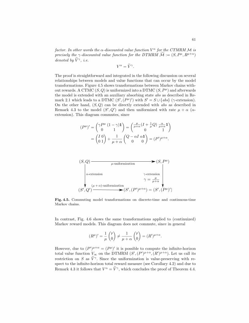
61
factor. In other words the α-discounted value function V α for the CTMRMM isprecisely the γ-discounted value function for the DTMRM M := (S, Pµ, Rµ+α)
denoted by V γ , i.e.
V α = V γ .
The proof is straightforward and integrated in the following discussion on severalrelationships between models and value functions that can occur by the modeltransformations. Figure 4.5 shows transformations between Markov chains with-out rewards. A CTMC (S,Q) is uniformized into a DTMC (S, Pµ) and afterwardsthe model is extended with an auxiliary absorbing state abs as described in Re-mark 2.1 which leads to a DTMC (S′, (Pµ)′) with S′ = S ∪abs (γ-extension).On the other hand, (S,Q) can be directly extended with abs as described inRemark 4.3 to the model (S′, Q′) and then uniformized with rate µ + α (α-extension). This diagram commutes, since
(Pµ)′ =
(γPµ (1− γ)1
0 1
)=
( µµ+α (I + 1
µQ) αµ+α1
0 1
)=
(I 00 1
)+
1
µ+ α
(Q− αI α1
0 0
)= (P ′)µ+α.
Fig. 4.5. Commuting model transformations on discrete-time and continuous-timeMarkov chains.
In contrast, Fig. 4.6 shows the same transformations applied to (continuized)Markov reward models. This diagram does not commute, since in general
(Rµ)′ =1
µ
(r0
)6= 1
µ+ α
(r0
)= (R′)µ+α.
However, due to (P ′)µ+α = (Pµ)′ it is possible to compute the infinite-horizontotal value function V∞ on the DTMRM (S′, (P ′)µ+α, (R′)µ+α). Let us call its
restriction on S as V γ . Since the uniformization is value-preserving with re-spect to the infinite-horizon total reward measure (see Corollary 4.2) and due to
Remark 4.3 it follows that V α = V γ , which concludes the proof of Theorem 4.4.
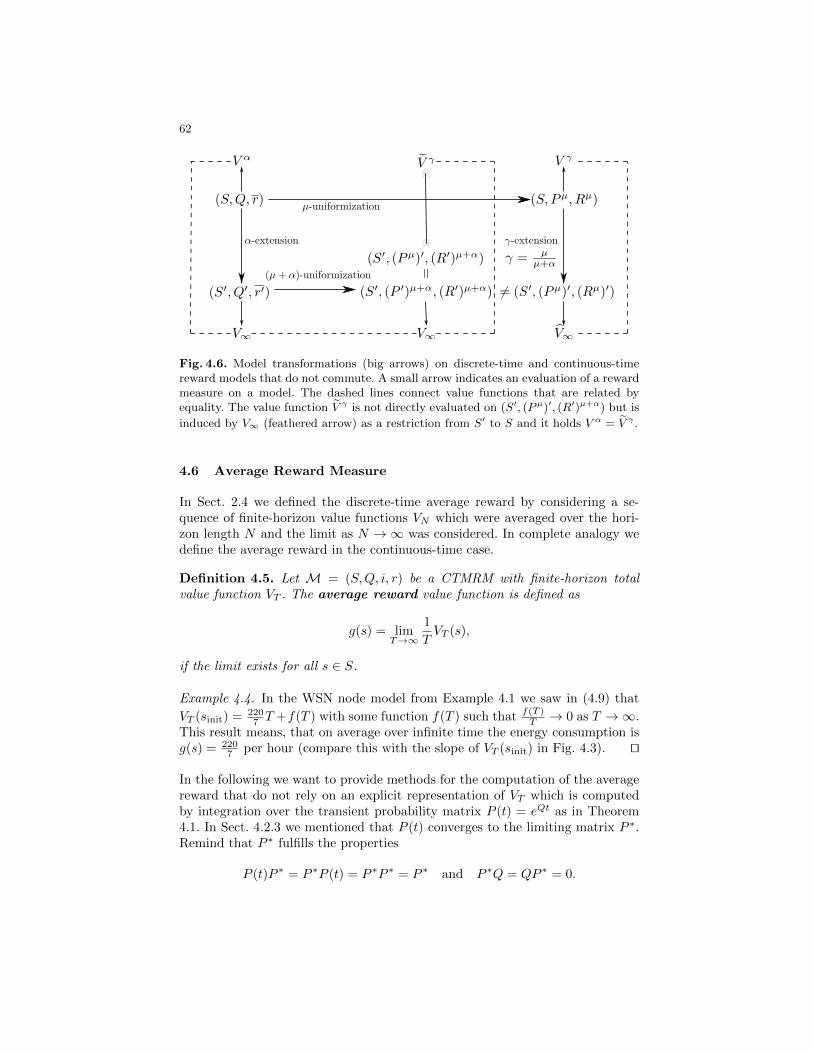
62
Fig. 4.6. Model transformations (big arrows) on discrete-time and continuous-timereward models that do not commute. A small arrow indicates an evaluation of a rewardmeasure on a model. The dashed lines connect value functions that are related byequality. The value function V γ is not directly evaluated on (S′, (Pµ)′, (R′)µ+α) but is
induced by V∞ (feathered arrow) as a restriction from S′ to S and it holds V α = V γ .
4.6 Average Reward Measure
In Sect. 2.4 we defined the discrete-time average reward by considering a se-quence of finite-horizon value functions VN which were averaged over the hori-zon length N and the limit as N →∞ was considered. In complete analogy wedefine the average reward in the continuous-time case.
Definition 4.5. Let M = (S,Q, i, r) be a CTMRM with finite-horizon totalvalue function VT . The average reward value function is defined as
g(s) = limT→∞
1
TVT (s),
if the limit exists for all s ∈ S.
Example 4.4. In the WSN node model from Example 4.1 we saw in (4.9) that
VT (sinit) = 2207 T +f(T ) with some function f(T ) such that f(T )
T → 0 as T →∞.This result means, that on average over infinite time the energy consumption isg(s) = 220
7 per hour (compare this with the slope of VT (sinit) in Fig. 4.3). ut
In the following we want to provide methods for the computation of the averagereward that do not rely on an explicit representation of VT which is computedby integration over the transient probability matrix P (t) = eQt as in Theorem4.1. In Sect. 4.2.3 we mentioned that P (t) converges to the limiting matrix P ∗.Remind that P ∗ fulfills the properties
P (t)P ∗ = P ∗P (t) = P ∗P ∗ = P ∗ and P ∗Q = QP ∗ = 0.

63
Proposition 4.2. Let r be the continuized rate reward of a CTMRM (S,Q, i, r).Then the average reward can be computed by
g = P ∗r.
Proof. By Theorem 4.1 it holds that
g = limT→∞
1
TVT = lim
T→∞
1
T
∫ T
0
P (t)r dt.
Fix two states s and s′ and consider the monotonically increasing function
h(T ) :=∫ T
0P (t)(s, s′) dt ≥ 0. If h(T ) is unbounded it follows by the rule of
l’Hospital that
limT→∞
h(T )
T= limT→∞
P (T )(s, s′) = P ∗(s, s′).
In the other case if h(T ) is bounded then clearly P (t)(s, s′) converges to 0. Butthis is only the case if either s and s′ are in different closed recurrent classes ors′ is transient and in both cases it holds that P ∗(s, s′) = 0. Thus from
limT→∞
h(T )
T= 0 = P ∗(s, s′)
the conclusion follows. ut
As in Sect. 2.4 we also show another possibility to evaluate the average rewardwhich does not rely on the computation of P ∗ and will be used in the subsequentsection on CTMDPs. For this reason we define the notion of a deviation matrixH and a bias h in the continuous-time case.
Definition 4.6. For a CTMRM M = (S,Q, i, r) define the deviation matrixH as
H :=
∫ ∞0
(P (t)− P ∗) dt,
where integration is performed componentwise. Further define
h := Hr =
∫ ∞0
(P (t)r − g) dt
as the bias of M.
Note that Q, H and P ∗ satisfy the following equations:
QH = HQ, P ∗ = I +QH and HP ∗ = P ∗H = 0. (4.18)
That can be easily derived by the Kolmogorov equations (4.2).In the following, we connect the discounted and the average reward measures.Consider for a fixed s ∈ S the discounted value V α(s) as a function of α ≥ 0.Then V α(s) might have a pole at α = 0 and can be extended as a Laurent seriesin α. For more information on the Laurent series expansion in continuous timewe refer to Theorem 7.1 in the Appendix. This theorem directly induces theLaurent series decomposition of the α-discounted value function as is stated inthe following corollary.
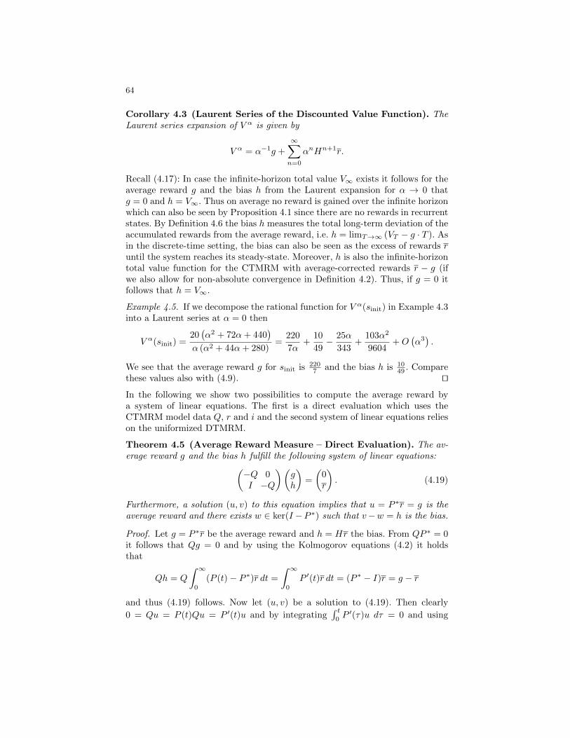
64
Corollary 4.3 (Laurent Series of the Discounted Value Function). TheLaurent series expansion of V α is given by
V α = α−1g +
∞∑n=0
αnHn+1r.
Recall (4.17): In case the infinite-horizon total value V∞ exists it follows for theaverage reward g and the bias h from the Laurent expansion for α → 0 thatg = 0 and h = V∞. Thus on average no reward is gained over the infinite horizonwhich can also be seen by Proposition 4.1 since there are no rewards in recurrentstates. By Definition 4.6 the bias h measures the total long-term deviation of theaccumulated rewards from the average reward, i.e. h = limT→∞ (VT − g · T ). Asin the discrete-time setting, the bias can also be seen as the excess of rewards runtil the system reaches its steady-state. Moreover, h is also the infinite-horizontotal value function for the CTMRM with average-corrected rewards r − g (ifwe also allow for non-absolute convergence in Definition 4.2). Thus, if g = 0 itfollows that h = V∞.
Example 4.5. If we decompose the rational function for V α(sinit) in Example 4.3into a Laurent series at α = 0 then
V α(sinit) =20(α2 + 72α+ 440
)α (α2 + 44α+ 280)
=220
7α+
10
49− 25α
343+
103α2
9604+O
(α3).
We see that the average reward g for sinit is 2207 and the bias h is 10
49 . Comparethese values also with (4.9). ut
In the following we show two possibilities to compute the average reward bya system of linear equations. The first is a direct evaluation which uses theCTMRM model data Q, r and i and the second system of linear equations relieson the uniformized DTMRM.
Theorem 4.5 (Average Reward Measure – Direct Evaluation). The av-erage reward g and the bias h fulfill the following system of linear equations:(
−Q 0I −Q
)(gh
)=
(0r
). (4.19)
Furthermore, a solution (u, v) to this equation implies that u = P ∗r = g is theaverage reward and there exists w ∈ ker(I −P ∗) such that v−w = h is the bias.
Proof. Let g = P ∗r be the average reward and h = Hr the bias. From QP ∗ = 0it follows that Qg = 0 and by using the Kolmogorov equations (4.2) it holdsthat
Qh = Q
∫ ∞0
(P (t)− P ∗)r dt =
∫ ∞0
P ′(t)r dt = (P ∗ − I)r = g − r
and thus (4.19) follows. Now let (u, v) be a solution to (4.19). Then clearly
0 = Qu = P (t)Qu = P ′(t)u and by integrating∫ t
0P ′(τ)u dτ = 0 and using
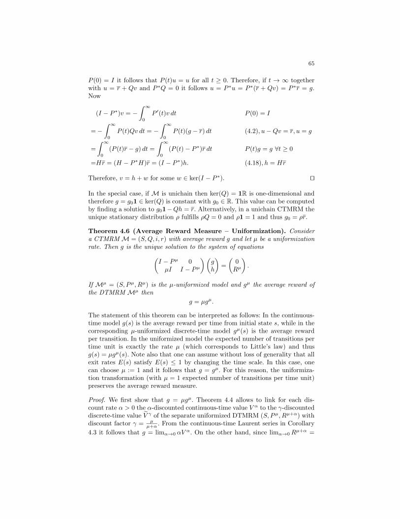
65
P (0) = I it follows that P (t)u = u for all t ≥ 0. Therefore, if t → ∞ togetherwith u = r + Qv and P ∗Q = 0 it follows u = P ∗u = P ∗(r + Qv) = P ∗r = g.Now
(I − P ∗)v = −∫ ∞
0
P ′(t)v dt P (0) = I
=−∫ ∞
0
P (t)Qv dt = −∫ ∞
0
P (t)(g − r) dt (4.2), u−Qv = r, u = g
=
∫ ∞0
(P (t)r − g) dt =
∫ ∞0
(P (t)− P ∗)r dt P (t)g = g ∀t ≥ 0
=Hr = (H − P ∗H)r = (I − P ∗)h. (4.18), h = Hr
Therefore, v = h+ w for some w ∈ ker(I − P ∗). ut
In the special case, if M is unichain then ker(Q) = 1R is one-dimensional andtherefore g = g01 ∈ ker(Q) is constant with g0 ∈ R. This value can be computedby finding a solution to g01−Qh = r. Alternatively, in a unichain CTMRM theunique stationary distribution ρ fulfills ρQ = 0 and ρ1 = 1 and thus g0 = ρr.
Theorem 4.6 (Average Reward Measure – Uniformization). Considera CTMRM M = (S,Q, i, r) with average reward g and let µ be a uniformizationrate. Then g is the unique solution to the system of equations(
I − Pµ 0µI I − Pµ
)(gh
)=
(0Rµ
).
If Mµ = (S, Pµ, Rµ) is the µ-uniformized model and gµ the average reward ofthe DTMRM Mµ then
g = µgµ.
The statement of this theorem can be interpreted as follows: In the continuous-time model g(s) is the average reward per time from initial state s, while in thecorresponding µ-uniformized discrete-time model gµ(s) is the average rewardper transition. In the uniformized model the expected number of transitions pertime unit is exactly the rate µ (which corresponds to Little’s law) and thusg(s) = µgµ(s). Note also that one can assume without loss of generality that allexit rates E(s) satisfy E(s) ≤ 1 by changing the time scale. In this case, onecan choose µ := 1 and it follows that g = gµ. For this reason, the uniformiza-tion transformation (with µ = 1 expected number of transitions per time unit)preserves the average reward measure.
Proof. We first show that g = µgµ. Theorem 4.4 allows to link for each dis-count rate α > 0 the α-discounted continuous-time value V α to the γ-discounteddiscrete-time value V γ of the separate uniformized DTMRM (S, Pµ, Rµ+α) withdiscount factor γ = µ
µ+α . From the continuous-time Laurent series in Corollary
4.3 it follows that g = limα→0 αVα. On the other hand, since limα→0R
µ+α =
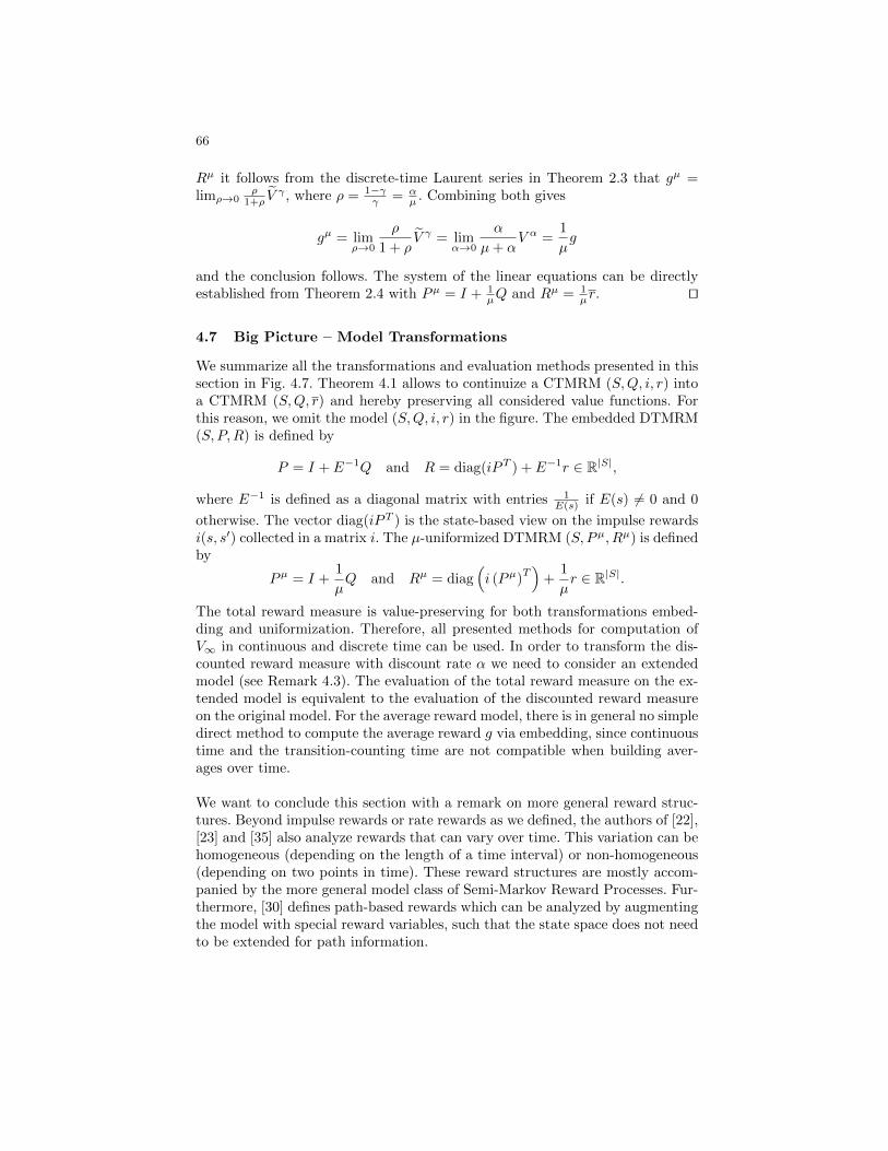
66
Rµ it follows from the discrete-time Laurent series in Theorem 2.3 that gµ =limρ→0
ρ1+ρ V
γ , where ρ = 1−γγ = α
µ . Combining both gives
gµ = limρ→0
ρ
1 + ρV γ = lim
α→0
α
µ+ αV α =
1
µg
and the conclusion follows. The system of the linear equations can be directlyestablished from Theorem 2.4 with Pµ = I + 1
µQ and Rµ = 1µr. ut
4.7 Big Picture – Model Transformations
We summarize all the transformations and evaluation methods presented in thissection in Fig. 4.7. Theorem 4.1 allows to continuize a CTMRM (S,Q, i, r) intoa CTMRM (S,Q, r) and hereby preserving all considered value functions. Forthis reason, we omit the model (S,Q, i, r) in the figure. The embedded DTMRM(S, P,R) is defined by
P = I + E−1Q and R = diag(iPT ) + E−1r ∈ R|S|,
where E−1 is defined as a diagonal matrix with entries 1E(s) if E(s) 6= 0 and 0
otherwise. The vector diag(iPT ) is the state-based view on the impulse rewardsi(s, s′) collected in a matrix i. The µ-uniformized DTMRM (S, Pµ, Rµ) is definedby
Pµ = I +1
µQ and Rµ = diag
(i (Pµ)
T)
+1
µr ∈ R|S|.
The total reward measure is value-preserving for both transformations embed-ding and uniformization. Therefore, all presented methods for computation ofV∞ in continuous and discrete time can be used. In order to transform the dis-counted reward measure with discount rate α we need to consider an extendedmodel (see Remark 4.3). The evaluation of the total reward measure on the ex-tended model is equivalent to the evaluation of the discounted reward measureon the original model. For the average reward model, there is in general no simpledirect method to compute the average reward g via embedding, since continuoustime and the transition-counting time are not compatible when building aver-ages over time.
We want to conclude this section with a remark on more general reward struc-tures. Beyond impulse rewards or rate rewards as we defined, the authors of [22],[23] and [35] also analyze rewards that can vary over time. This variation can behomogeneous (depending on the length of a time interval) or non-homogeneous(depending on two points in time). These reward structures are mostly accom-panied by the more general model class of Semi-Markov Reward Processes. Fur-thermore, [30] defines path-based rewards which can be analyzed by augmentingthe model with special reward variables, such that the state space does not needto be extended for path information.
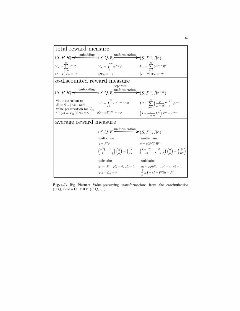
67
Fig. 4.7. Big Picture: Value-preserving transformations from the continuization(S,Q, r) of a CTMRM (S,Q, i, r).
68
5 Continuous Time Markov Decision Processes
In this section we merge both model types MDP and CTMRM together into aCTMDP model. This section is rather short, because all of the necessary workhas been already done in the preceding sections. For this reason, we establishconnections to the previous results. Moreover, we also present an additionalmethod for the computation of the average reward which directly works onCTMDPs.
5.1 Preliminaries and Retrospection
Definition 5.1. A continuous-time Markov Decision Process (CTMDP)is a structureM = (S,Act, e,Q, i, r), where S is a finite state space, Act a finiteset of actions, e : S → 2Act \∅ the action-enabling function, Q : S×Act×S → Ran action-dependent generator function, i : S×Act×S → R the action-dependentimpulse reward function with i(s, a, s) = 0 for all a ∈ e(s) and r : S × Act → Rthe action-dependent rate reward function.
Completely analogous to Sect. 3 we define the set of policies
Π := π : S → Act | π(s) ∈ e(s) .
Applying π to a CTMDP M induces a CTMRM Mπ = (S,Qπ, iπ, rπ), where
Qπ(s, s′) := Q(s, π(s), s′), iπ(s, s′) := i(s, π(s), s′) and rπ(s) := r(s, π(s)).
A reward measure R for the CTMDP M induces for each policy π a value V π
for Mπ.
Definition 5.2. Let M be a CTMDP with reward measure R and for eachπ ∈ Π let V π be the value of π with respect to R. The value V ∗ of M is definedas
V ∗(s) := supπ∈Π
V π(s).
A policy π∗ ∈ Π is called optimal if
∀s ∈ S ∀π ∈ Π : V π∗(s) ≥ V π(s).
In order to optimize the CTMDP we can transform M by embedding or uni-formization into an MDP and by continuization into another CTMDP. The trans-formations follow the Big Picture as presented in Sect. 4.7 (Fig. 4.7) with thedifference that all action-dependent quantities (i.e. Q, i and r) are transformed inan action-wise manner. The following theorem states that these transformationspreserve both the optimal value and the optimal policies.
Theorem 5.1. LetM be a CTMDP with policy space Π, optimal value V ∗ anda set of optimal policies Π∗ ⊆ Π. Further let M be a transformed model (MDP
or CTMDP) as in Fig. 4.7 with policy space Π, value V ∗ and optimal policies
Π∗ ⊆ Π. ThenV ∗ = V ∗ and Π∗ = Π∗.
69
Proof. Note that V ∗ and V ∗ are defined over policies, i.e.
V ∗ = supπ∈Π
V π and V ∗ = supπ∈Π
V π.
All the transformations in Fig. 4.7 do not transform S, Act and e, thus Π = Π.Furthermore, for each π ∈ Π the transformations preserve the value V π, i.e.V π = V π and thus V ∗ = supπ∈Π V
π = supπ∈Π Vπ = V ∗. In order to show that
Π∗ = Π∗ let π∗ ∈ Π∗. Then for all s and for all π ∈ Π by definition of π∗ itholds that
V π∗(s) ≥ V π(s) = V π(s) and V π
∗(s) = V π
∗(s).
and therefore π∗ is optimal for M , i.e. π∗ ∈ Π∗. In complete analogy it followsthat Π∗ ⊆ Π∗ and the equality for the sets of optimal policies follows. ut
5.2 Average Reward Measure
All the necessary work has already been done for analyzing CTMDPs by trans-formation to MDPs. It remains to provide optimality equations for the averagereward and algorithms which can be used directly on CTMDPs. Consider aCTMDP (S,Act, e,Q, i, r) with average reward measure and let
r(s, a) =∑s′ 6=s
i(s, a, s′)Q(s, a, s′) + r(s, a)
denote the continuized rate reward. Define the Bellman operators Bav : RS → RSand Bgbias : RS → RS (parametrized by g ∈ RS) as follows:
(Bavg)(s) := maxa∈e(s)
∑s′∈S
Q(s, a, s′)g(s′)
(Bgbiash)(s) := maxa∈eg(s)
r(s, a) +
∑s′∈S
Q(s, a, s′)h(s′)
− g(s)
where eg(s) :=
a ∈ e(s) |
∑s′∈S
Q(s, a, s′)g(s′) = 0
These operators look similar to the Bellman operators (3.10) and (3.11) in thediscrete-time case. The difference is that instead of searching for fixed-points weneed to search for zeros of Bav and Bgbias (see (4.19)). This gives the first and thesecond Bellman optimality equations
maxa∈e(s)
∑s′∈S
Q(s, a, s′)g(s′)
= 0 (5.1)
maxa∈eg(s)
r(s, a) +
∑s′∈S
Q(s, a, s′)h(s′)
− g(s) = 0. (5.2)
70
The following existence theorem is the analogue version of Theorem 5.2 fordiscrete-time MDPs.
Theorem 5.2 (Existence Theorem).
(i) The average optimal value function g∗ is a solution to (5.1), i.e Bavg∗ = 0.
For g = g∗ there exists a solution h to (5.2), i.e. Bg∗
biash = 0. If g and h aresolutions to (5.1) and (5.2) then g = g∗.
(ii) There exists an optimal policy π∗ and it holds that gπ∗
= g∗.(iii) For any solution h to (5.2) with g = g∗ an optimal policy π∗ can be derived
from
π∗(s) ∈ argmaxa∈eg∗ (s)
r(s, a) +
∑s′∈S
Q(s, a, s′)h(s′)
.
For a direct proof we refer to [17]. We propose here another proof sketch basedon uniformization and its value-preserving property.
Proof. Without loss of generality we assume that E(s, a) ≤ 1 and set the uni-formization rate µ := 1 such that the uniformization is value-preserving. Theµ-uniformized MDP is given by Mµ = (S,Act, e, Pµ, Rµ) where
Pµ(s, a, s′) = δs,s′ +Q(s, a, s′) and Rµ(s, a) = r(s, a).
If (gµ)∗ denotes the optimal average reward forMµ then by Theorem 5.1 it holdsthat g∗ = (gµ)∗. Since finding a fixed point of some operator T is equivalent tofinding a zero of the operator B = T − id, where id is the identity operator, part(i) follows. Furthermore, Theorem 3.7 guarantees the existence of an optimalpolicy for Mµ and by Theorem 5.1 also for M such that parts (ii) and (iii)follow. ut
We restate the policy iteration algorithm from [17] since our CTMDP model asintroduced in Definition 5.1 allows also impulse rewards.
Theorem 5.3 (Policy Iteration). Let M = (S,Act, e,Q, i, r) be a CTMDPand r(s, a) the continuized rate reward. For an initial policy π0 ∈ Π define thefollowing iteration scheme:
1. Policy evaluation: Compute a solution (gπn , hπn , w)T
to−Qπn 0 0I −Qπn 00 I −Qπn
gπnhπn
w
=
0rπn
0
2. Policy improvement: Define for each state s the set of improving actions
Bn+1(s) :=
a ∈ e(s) |∑s′ Q(s, a, s′)gπn(s′) > 0 ∨
(∑s′ Q(s, a, s′)gπn(s′) = 0⇒ r(s, a) +
∑s′ Q(s, a, s′)hπn(s′) > gπn(s))
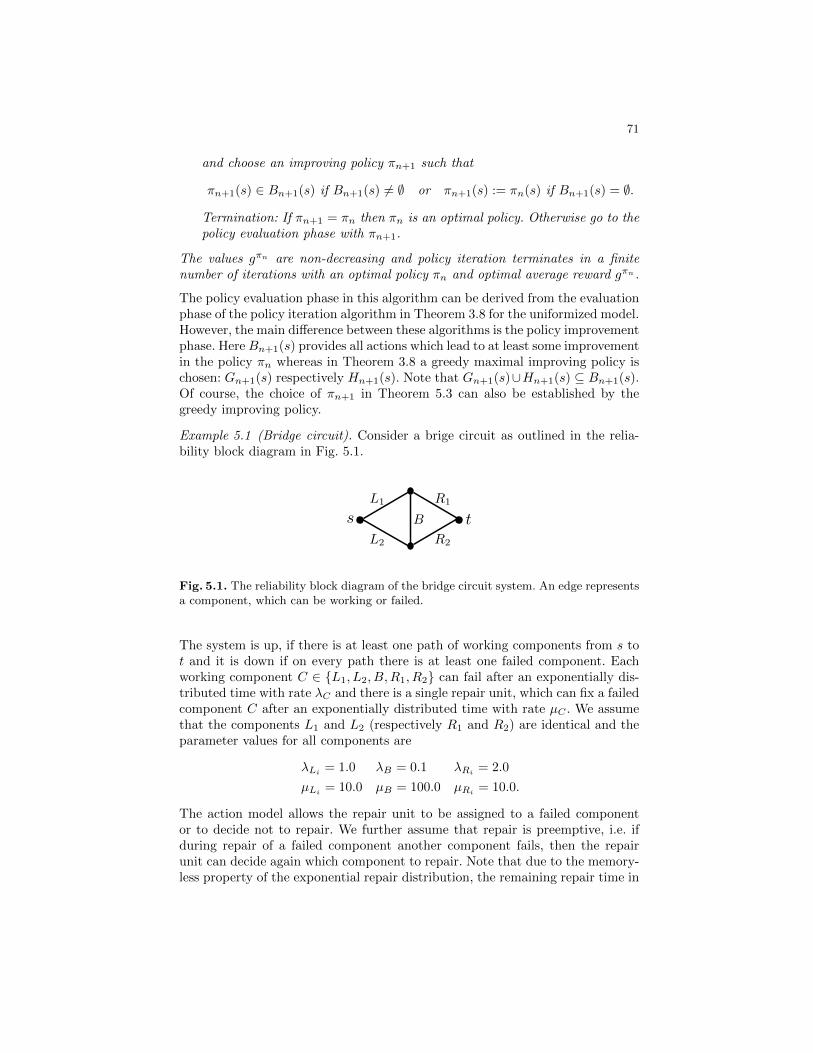
71
and choose an improving policy πn+1 such that
πn+1(s) ∈ Bn+1(s) if Bn+1(s) 6= ∅ or πn+1(s) := πn(s) if Bn+1(s) = ∅.
Termination: If πn+1 = πn then πn is an optimal policy. Otherwise go to thepolicy evaluation phase with πn+1.
The values gπn are non-decreasing and policy iteration terminates in a finitenumber of iterations with an optimal policy πn and optimal average reward gπn .
The policy evaluation phase in this algorithm can be derived from the evaluationphase of the policy iteration algorithm in Theorem 3.8 for the uniformized model.However, the main difference between these algorithms is the policy improvementphase. HereBn+1(s) provides all actions which lead to at least some improvementin the policy πn whereas in Theorem 3.8 a greedy maximal improving policy ischosen: Gn+1(s) respectively Hn+1(s). Note that Gn+1(s)∪Hn+1(s) ⊆ Bn+1(s).Of course, the choice of πn+1 in Theorem 5.3 can also be established by thegreedy improving policy.
Example 5.1 (Bridge circuit). Consider a brige circuit as outlined in the relia-bility block diagram in Fig. 5.1.
Fig. 5.1. The reliability block diagram of the bridge circuit system. An edge representsa component, which can be working or failed.
The system is up, if there is at least one path of working components from s tot and it is down if on every path there is at least one failed component. Eachworking component C ∈ L1, L2, B,R1, R2 can fail after an exponentially dis-tributed time with rate λC and there is a single repair unit, which can fix a failedcomponent C after an exponentially distributed time with rate µC . We assumethat the components L1 and L2 (respectively R1 and R2) are identical and theparameter values for all components are
λLi = 1.0 λB = 0.1 λRi = 2.0
µLi = 10.0 µB = 100.0 µRi = 10.0.
The action model allows the repair unit to be assigned to a failed componentor to decide not to repair. We further assume that repair is preemptive, i.e. ifduring repair of a failed component another component fails, then the repairunit can decide again which component to repair. Note that due to the memory-less property of the exponential repair distribution, the remaining repair time in

72
order to complete the repair does not depend on the elapsed time for repair. Wewant to find optimal repair policies, in order to pursue the following two goals:
(G1): maximize the MTTF (mean time to failure)(G2): maximize the availability (i.e. the fraction of uptime in the total time).
Figure 5.2 shows an excerpt of the state space (with 32 states), which we applyto both goals (G1) and (G2). Note that for both measures (MTTF and avail-ability) we define the reward structure which consists only of the rate reward r,which is 1 on up states and 0 on down states. The difference between both goalsaffects the state space as follows: For (G1) the 16 down states are absorbing(for every policy), while for (G2) a repair of failed components is also allowed indown system states.
11111
idle
01111 10111 11011 11101 11110
01011repL1repB
idle
00011 01001 01010
Fig. 5.2. State space of the bridge circuit CTMDP model. State encoding 01011 repre-sents (from left to right) that L1 has failed, L2 is working, B has failed, R1 is workingand R2 is working. From every state where at least some component has failed, thereare repair actions and from each state there is also the idle action indicating that therepair unit can choose not to repair. Shadowed states represent down system states.
We optimize (G1) by transforming the CTMDP by embedding into a discrete-time SSP (S, P,R) (cf. Definition 3.4 and Fig. 4.7) and hereby aggregate allabsorbing down states to the goal state for the SSP. By embedding transforma-tion, the reward R(s, a) is the expected sojourn time in state s under action a
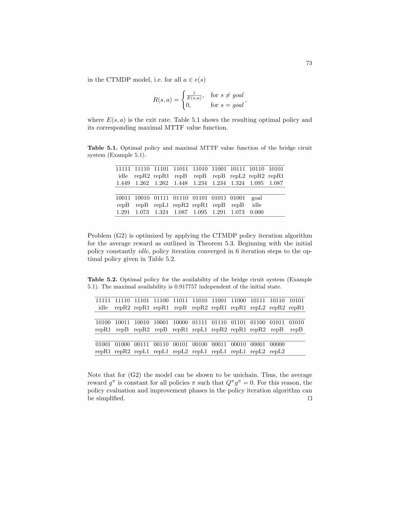
73
in the CTMDP model, i.e. for all a ∈ e(s)
R(s, a) =
1
E(s,a) , for s 6= goal
0, for s = goal,
where E(s, a) is the exit rate. Table 5.1 shows the resulting optimal policy andits corresponding maximal MTTF value function.
Table 5.1. Optimal policy and maximal MTTF value function of the bridge ciruitsystem (Example 5.1).
11111 11110 11101 11011 11010 11001 10111 10110 10101idle repR2 repR1 repB repB repB repL2 repR2 repR1
1.449 1.262 1.262 1.448 1.234 1.234 1.324 1.095 1.087
10011 10010 01111 01110 01101 01011 01001 goalrepB repB repL1 repR2 repR1 repB repB idle1.291 1.073 1.324 1.087 1.095 1.291 1.073 0.000
Problem (G2) is optimized by applying the CTMDP policy iteration algorithmfor the average reward as outlined in Theorem 5.3. Beginning with the initialpolicy constantly idle, policy iteration converged in 6 iteration steps to the op-timal policy given in Table 5.2.
Table 5.2. Optimal policy for the availability of the bridge ciruit system (Example5.1). The maximal availability is 0.917757 independent of the initial state.
11111 11110 11101 11100 11011 11010 11001 11000 10111 10110 10101idle repR2 repR1 repR1 repB repR2 repR1 repR1 repL2 repR2 repR1
10100 10011 10010 10001 10000 01111 01110 01101 01100 01011 01010repR1 repB repR2 repB repR1 repL1 repR2 repR1 repR2 repB repB
01001 01000 00111 00110 00101 00100 00011 00010 00001 00000repR1 repR2 repL1 repL1 repL2 repL1 repL1 repL1 repL2 repL2
Note that for (G2) the model can be shown to be unichain. Thus, the averagereward gπ is constant for all policies π such that Qπgπ = 0. For this reason, thepolicy evaluation and improvement phases in the policy iteration algorithm canbe simplified. ut
74
6 Conclusion and Outlook
In this tutorial, we presented an integrated picture of MRMs and MDPs overfinite state spaces for both discrete and continuous time. The theory and appli-cation area for this kind of models is very popular and broad. For this reason, wejust focussed on the fundamentals of the theory. We reviewed the most impor-tant basic facts from literature, which are inevitable for a deeper understandingof Markovian models. Furthermore, we set up the theory step by step fromdiscrete-time MRMs up to continuous-time MDPs and pointed out importantlinks between these theories. We also connected these models by a number ofmodel transformations and highlighted their properties. In order to show the ap-plicability of these models, we introduced small prototypical examples, comingfrom the domain of performance and dependability evaluation and optimization.Of course, many current applications in the optimization of dependable systemssuffer from the curse of dimensionality. However, there are established tech-niques which can be used in order to overcome this curse and make evaluationand optimization for large practical models accessible, e.g. approximate solutions(e.g. approximate dynamic programming), simulative approaches (reinforcementlearning) or the use of structured models. There are also several important ex-tensions to the Markov model types we could not address in this introductorytutorial, such as partially observable MDPs (used especially in the area of AI),denumerable state and action spaces (e.g. for queueing systems) or even contin-uous state and action spaces (leading directly to control theory).
75
7 Appendix
7.1 Lemmata and Remarks
Lemma 7.1.
(i) Let N be a non-negative discrete random variable with expected value and(an)n∈N a bounded sequence. Then
E
[N∑n=0
an
]=
∞∑n=0
anP (N ≥ n).
(ii) Let T be a non-negative continuous random variable with expected value anda : [0,∞)→ R an integrable and bounded function. Then
E
[∫ T
0
a(t) dt
]=
∫ ∞0
a(t)P (T ≥ t) dt.
Proof. We show only (i) – the proof for (ii) is analogous when summation isreplaced by integration. Since an is bounded and E [N ] =
∑∞n=0 P (N ≥ n) <∞
it follows that∑∞n=0 anP (N ≥ n) converges absolutely. From
∞∑n=0
anP (N ≥ n) =
∞∑n=0
∞∑k=n
anP (N = k) =
∞∑n=0
∞∑k=0
anP (N = k)1k≥n(n, k)
we can interchange both infinite summations by the Fubini theorem. It follows
∞∑n=0
anP (N ≥ n) =
∞∑k=0
∞∑n=0
anP (N = k)1n≤k(n, k)
=
∞∑k=0
k∑n=0
anP (N = k) = E
[N∑n=0
an
]. ut
Remark 7.1. As presented in Sect. 4.2.2 a CTMC M = (S,Q) induces thestochastic processes Xn, τn, Tn, Nt and Zt. If we fix a uniformization rate µ > 0then M also induces the uniformized stochastic processes Xn, τn, Tn, Ntand Zt over Ω = (S × (0,∞])N. Here Xn is the n-th visited state in the uni-
formized DTMC and τn is the time up to transition in state Xn, i.e. all τnare independent and exponentially distributed with rate µ. Moreover, the totalelapsed time Tn :=
∑n−1k=0 τk for the first n transitions is Erlang distributed with
n phases and rate µ and the number Nt := maxn | Tn(ω) ≤ t of (uniformized)transitions up to time t ≥ 0 is Poisson distributed with parameter µt. Notealso that Zt := XNt
= XNt = Zt for all t ≥ 0. Thus, when uniformization isconsidered as adding exponentially distributed self-loop transitions to states ofthe CTMC M, then the continuous-time state process Zt is not modified atall. Therefore, the probability measures Ps of the CTMC for all s ∈ S are leftinvariant under uniformization and especially the transient probability matrixP (t) as defined in (4.1). ut
76
Lemma 7.2. Consider a CTMCM= (S,Q) with discrete-time and continuous-time state processes Xn and Zt. Let
nT (s, s′) := Es0
[NT∑k=1
1Xk−1=s,Xk=s′
]
be the expected number of transitions from state s to state s′ 6= s within the timeinterval [0, T ] from a fixed initial state X0 = s0. Then
nT (s, s′) = Q(s, s′)
∫ T
0
Ps0(Zt = s) dt. (7.1)
Proof. If s is absorbing then clearly (7.1) holds and we can assume in the fol-lowing that E(s) > 0. We abbreviate in the following the notation by E := Es0and P := Ps0 . Define
nT (s) :=∑s′ 6=s
nT (s, s′) = E
[NT∑k=1
1Xk−1=s
]=
∞∑k=1
P (Xk−1 = s)P (NT ≥ k)
as the number of complete visits to state s, such that s has been left before timeT . From P (Xk−1 = s,Xk = s′) = P (Xk = s′|Xk−1 = s)P (Xk−1 = s) it followsthat
nT (s, s′) = P (s, s′)
∞∑k=1
P (Xk−1 = s)P (NT ≥ k) = P (s, s′)nT (s),
where P (s, s′) = δs,s′ + Q(s,s′)E(s) is the embedded transition probability. We use
uniformization as means for proof with a uniformization rate µ ≥ maxs∈S E(s).
Let Xk, τk, Tk and Nt be the uniformized stochastic processes as defined in
Remark 7.1. Then Tk is Erlang distributed with density fTk(t) = e−µt µktk−1
(k−1)! for
t ≥ 0 and Nt has the Poisson probabilities P (Nt = k) = e−µt (µt)k
k! . The totalaccumulated time for complete visits in s up to time T fulfills
1
E(s)E
[NT∑k=1
1Xk−1=s
]=
1
µE
NT∑k=1
1Xk−1=s
and therefore
nT (s) =E(s)
µE
NT∑k=1
1Xk−1=s
77
is a fraction of the number of uniformized transitions up to time T from state sto some arbitrary state s′. It follows that
nT (s) =E(s)
µE
NT∑k=1
1Xk−1=s
=E(s)
µ
∞∑k=1
P (Xk−1 = s)P (NT ≥ k)
=E(s)
µ
∞∑k=0
P (Xk = s)P (Tk+1 ≤ T )
=E(s)
µ
∞∑k=0
P (Xk = s)
∫ T
0
e−µtµk+1tk
k!dt
= E(s)
∫ T
0
e−µt∞∑k=0
P (Xk = s)(µt)k
k!dt = E(s)
∫ T
0
P (Zt = s) dt
since
P (Zt = s) =
∞∑k=0
P (Zt = s | Nt = k)P (Nt = k) =
∞∑k=0
P (Xk = s)e−µt(µt)k
k!.
Thus, (7.1) follows from P (s, s′) = Q(s,s′)E(s) for s′ 6= s and nT (s, s′) =P (s, s′)nT (s).
ut
Remark 7.2. In the proof of Lemma 7.2, we have applied uniformization as adetour in order to show that
nT (s, s′) = Q(s, s′)
∫ T
0
Ps0(Zt = s) dt.
There is also a more direct way to show this equation by an argument that is usedin the proof of the PASTA property (“Poisson Arrivals See Time Averages”) [41].The PASTA property is a tool that is frequently used in the theory of queueingsystems. Consider a system that is represented by the Markov chainM = (S,Q)with state process Zt for t ≥ 0 and fix two states s and s′ with Q(s, s′) > 0.Let τs,s′ be the exponentially distributed time with rate Q(s, s′) that governsthe transition from s to s′ as shown in Sect. 4.1. Further define an independent
sequence of such random variables τ(n)s,s′ , n ∈ N with same distribution as τs,s′ .
Then the process At := maxn |∑n−1k=0 τ
(k) ≤ t
is a Poisson process with rate
Q(s, s′) and is regarded as a stream of arriving jobs to the system. Since τs,s′
is memoryless it holds that when the system is in state s and an arrival occursthen the system performs a transition to s′. Therefore, the counting processYt :=
∑Ntk=1 1Xk−1=s,Xk=s′ is precisely the number of arrivals of At to the
system (up to time t) that find the system in state s. Further let Ut := 1Zt=sbe the process that indicates whether the system is in state s at time t. Itholds that Yt can be represented as a stochastic Riemann-Stiltjes integral of theprocess Ut with respect to the arrival process At, i.e. for all T ≥ 0 it holds
78
that YT =∫ T
0Ut dAt with probability 1. Note that for each t ≥ 0 the set of
future increments At+s −As | s ≥ 0 and the history of the indicator processUs | 0 ≤ s ≤ t are independent. Thus the “lack of anticipation assumption” asneeded for [41] is satisfied and it follows that
nT (s, s′) = Es0 [YT ] = Q(s, s′) · Es0
[∫ T
0
Ut dt
]= Q(s, s′)
∫ T
0
Ps0(Zt = s) dt.
ut
Lemma 7.3. Let T be a non-negative continuous random horizon length for aCTMRMM = (S,Q, i, r) and independent of the state process Zt ofM. Furtherlet NT = max n | Tn ≤ T be the random number of transitions up to time T .If the k-th moment of T exists, then it also exists for NT .
In order to prove this theorem we need the following definition.
Definition 7.1. For two random variables X and Y with distributions FX andFY we say that X is stochastically smaller then Y (denoted by X Y ) ifFX(x) ≥ FY (x) for all x ∈ R.
It follows that if X Y then E [g(X)] ≤ E [g(Y )] for a monotonically increasingfunction g.
Proof. Let Xn, τn, Tn and Nt be the stochastic processes as defined in Sect. 4.2.2.Further choose µ := max E(s) | s ∈ S as a uniformization rate and Xn, τn, Tnand Nt the uniformized processes as in Remark 7.1. First we show thatNT NT :From µ ≥ E(s) for all s it follows that τn τn for all n and thus Tn Tn.Therefore
NT = maxn | Tn ≤ T maxn | Tn ≤ T = NT
and thus E[NkT ] ≤ E[Nk
T ]. In order to show that E[NkT ] is finite we show E[Nk
T ] <
∞. It holds that P (NT = n) = P (Tn ≤ T < Tn+1) and therefore
E[NkT ] =
∞∑n=0
nkP (Tn ≤ T < Tn+1).
We show that the sequence P (Tn ≤ T < Tn+1) is decreasing fast enough.
P (Tn ≤ T < Tn+1) =
∫ ∞z=0
fT (z)
∫ z
v=0
fTn(v)
∫ ∞u=z−v
fτn(u) du dv dz =∫ ∞z=0
fT (z)
∫ z
v=0
fTn(v)e−µ(z−v) dv dz =
∫ ∞z=0
fT (z)e−µz∫ z
v=0
µnvn−1
(n− 1)!dv dz =∫ ∞
z=0
fT (z)e−µz(µz)n
n!dz.
Therefore
E[NkT ] =
∞∑n=0
nk∫ ∞z=0
fT (z)e−µz(µz)n
n!dz =
∫ ∞z=0
fT (z)E[Nkz ] dz,
79
where Nz is the number of uniformized transitions up to time z which is Pois-son distributed with parameter µz. Now the k-th moment g(z) := E[Nk
z ] is apolynomial in z of degree k and therefore
E[NkT ] =
∫ ∞z=0
g(z)fT (z) dz <∞,
as a polynomial of degree k in the moments of T . ut
Remark 7.3. In the case k = 1 it holds that E[NT ] = µE [T ] represents exactlyLittle’s law: If jobs enter a queue at rate µ and if their mean residence time inthe queue is E [T ], then there are on average µE [T ] jobs in the queue. For k ≥ 2
the theorem generalizes Little’s law and allows to compute E[NT ] analyticallysince the coefficients of g can be computed analytically.
7.2 Laurent Series Expansion for Continuous Time Models
Proposition 7.1. Let Q ∈ Rn×n be the generator matrix of a CTMC over afinite state space and P (t) = eQt the transient probability matrix. Then theCTMC is exponentially ergodic, i.e. there exists δ > 0 and L > 0, such that
||P (t)− P ∗|| ≤ Le−δt
for all t ≥ 0, where ||A|| := maxi∑j |Ai,j | is the matrix maximum norm.
In [18] an equivalent statement is described for finite state DTMCs. We transferand modify the proof to the continuous-time case.
Proof. Since Pi,j(t)→ P ∗i,j for all i, j, it follows that for an arbitrary fixed ε > 0there exists T > 0, such that for all i∑
j
|Pi,j(T )− P ∗i,j | ≤ e−ε < 1
and therefore ||P (T ) − P ∗|| ≤ e−ε. Now split t = ntT + st with nt ∈ N andst ∈ [0, T ).
||P (t)− P ∗|| = ||P (T )ntP (st)− P ∗|| P (s+ t) = P (s)P (t)
= || (P (T )nt − P ∗) (P (st)− P ∗) || P (t)P ∗ = P ∗, P ∗P ∗ = P ∗
≤ ||P (T )nt − P ∗|| · ||P (st)− P ∗|| subadditivity of norm
= || (P (T )− P ∗)nt || · ||P (st)− P ∗||≤ ||P (T )− P ∗||nt · ||P (st)− P ∗||≤ e−εnt ||P (st)− P ∗||= e−εt/T eεst/T ||P (st)− P ∗||.
Defining
δ :=ε
Tand L := sup
s∈[0,T )
(eεs/T ||P (s)− P ∗||
)<∞
gives ||P (t)− P ∗|| ≤ Le−δt. ut
80
Define the transient deviation matrix ∆(t) := P (t)−P ∗ and the total deviationmatrix H :=
∫∞0∆(t) dt (componentwise integration). From Proposition 7.1 it
follows that the integral defining H converges since ||∆(t)|| ≤ Le−δt.
Theorem 7.1. For α > 0 let W (α) :=∫∞
0e−αtP (t) dt be the Laplace transform
of P (t). Then there exists δ > 0, such that for all 0 < α < δ the Laurent seriesof W (α) is given by
W (α) = α−1P ∗ +
∞∑n=0
(−α)nHn+1.
Proof. Since P (t)P ∗ = P ∗P (t) = P ∗P ∗ = P ∗ it follows that ∆(t+s) = ∆(t)∆(s)for all s, t ≥ 0. Now
W (α) =
∫ ∞0
e−αt(P (t)− P ∗ + P ∗) dt
= α−1P ∗ +
∫ ∞0
e−αt∆(t) dt
= α−1P ∗ +
∫ ∞0
( ∞∑n=0
(−αt)n
n!
)∆(t) dt
= α−1P ∗ +
∞∑n=0
(−α)n∫ ∞
0
tn
n!∆(t) dt,
where the last equality follows from Lebesgue’s dominated convergence theorem,
since for all i, j the sequence∑Nn=0
(−αt)nn! ∆i,j(t) can be dominated by the inte-
grable function Ce(α−δ)t (for δ > 0 from Proposition 7.1 and some C > 0) forall 0 < α < δ. We show by induction that∫ ∞
0
tn
n!∆(t) dt = Hn+1. (7.2)
For n = 0 this is true by definition of H. Let (7.2) be true for an arbitrary n ∈ N.Then∫ ∞
0
tn+1
(n+ 1)!∆(t) dt =
∫ ∞0
(∫ t
0
sn
n!ds
)∆(t) dt =
∫ ∞0
sn
n!
∫ ∞s
∆(t) dt ds
=
∫ ∞0
sn
n!
∫ ∞0
∆(s+ t) dt ds =
∫ ∞0
sn
n!∆(s)
∫ ∞0
∆(t) dt ds
=
(∫ ∞0
sn
n!∆(s) ds
)H = Hn+1
and the Laurent series follows. ut
81
7.3 Collection of Proofs
Proof (of Theorem 2.1). (i) For an arbitary s0 ∈ S it holds
VN (s0) = Es0
[N∑i=1
R(Xi−1, Xi)
]=
∑s1,...,sN
((N∑i=1
R(si−1, si)
)N∏i=1
P (si−1, si)
)
=∑s1
P (s0, s1)
(R(s0, s1)
∑s2,...,sN
N∏i=2
P (si−1, si) +
∑s2,...,sN
N∑i=2
R(si−1, si)
N∏i=2
P (si−1, si)
).
Now since∑s1R(s0, s1)P (s0, s1) = R(s0) and for each s1 ∈ S it holds that
∑s2,...,sN
N∏i=2
P (si−1, si) = 1 and
∑s2,...,sN
(N∑i=2
R(si−1, si)
)N∏i=2
P (si−1, si) = Es1
[N∑i=2
R(Xi−1, Xi)
]= VN−1(s1)
it follows thatVN (s0) = R(s0) +
∑s1
P (s0, s1)VN−1(s1).
In case V∞ exists then V∞(s) = limN→∞ VN (s) for all s ∈ S and statement (ii)follows from (i) by taking the limit on both sides. ut
Proof (of Proposition 2.1). We are going to sketch a proof for this fact in casethe Markov chain is aperiodic. Since V∞ exists for the model (S, P,R) if andonly if it exists for (S, P, |R|) we can assume without loss of generality thatR(s, s′) ≥ 0 for all s, s′ ∈ S. Note that here |R| has to be interpreted as thetransition-based reward function with |R|(s, s′) := |R(s, s′)|. The reason is thatthe state-based view on the absolute reward values
∑s′∈S P (s, s′)|R(s, s′)| in
general differs from |∑s′∈S P (s, s′)R(s, s′)| which is the absolute value of the
state-based view on the reward values!“⇒”: Assume that V∞ exists and R(s, s′) > 0 for some states s, s′ ∈ Sri and thusR(s) =
∑s′∈S P (s, s′)R(s, s′) > 0. For all k ∈ N it holds that Es [R(Xk−1, Xk)]
is the reward gained for the k-th transition when starting in s. Therefore
Es [R(Xk−1, Xk)] =∑s′∈S
P k−1(s, s′)∑s′′∈S
P (s′, s′′)R(s′, s′′)
=∑s′∈S
P k−1(s, s′)R(s′) ≥ P k−1(s, s)R(s).
Since P is aperiodic and s is recurrent it follows that P k−1(s, s) converges toρs(s) > 0, where ρs is the limiting distribution from s (see Sect. 2.1.2). Therefore
82
the sequence Es[∑N
k=1 |R(Xk−1, Xk)|]≥∑Nk=1 P
k−1(s, s)R(s) is unbounded,
which is a contradiction to the existence of V∞.“⇐”: Assume that R(s, s′) = 0 for all s, s′ ∈ Sri and all i = 1, . . . , k. Weanticipate a result from Proposition 2.2 in Sect. 2.4, which states that the limitingmatrix P∞ := limn→∞ Pn exists since P is aperiodic. In [18] it is shown that Pis geometric ergodic, i.e. there exists n0 ∈ N, c > 0 and β < 1 such that
||Pn − P∞|| ≤ cβn
for all n ≥ n0, where ||.|| is the maximum norm. (This result as stated holds forunichain models, but it can also be directly extended to the multichain case).First of all, we want to show that P∞R = 0, i.e. for all s ∈ S it holds that
(P∞R)(s) =∑s′∈S
P∞(s, s′)∑s′′∈S
P (s′, s′′)R(s′, s′′) = 0.
If s ∈ Sri is recurrent then we only have to consider those terms in the summationfor which s′ and s′′ are in the same closed recurrent class Sri . But since boths′, s′′ ∈ Sri it follows that R(s′, s′′) = 0 and thus (P∞R)(s) = 0. On the otherhand if s ∈ St is transient then P∞(s, s′) = 0 for all s′ ∈ St and otherwise if s′ isrecurrent then again P (s′, s′′) = 0 or R(s′, s′′) = 0 dependent on whether s′ ands′′ are in the same closed recurrent class. (Compare this also to the representationof P∞ = P ∗ in (2.14).) Combining together it follows for all s ∈ S and k ≥ n0+1that
Es [R(Xk−1, Xk)] =∑s′∈S
P k−1(s, s′)∑s′′∈S
P (s′, s′′)R(s′, s′′) =∑s′∈S
P k−1(s, s′)R(s′)
≤ maxs∈S
∑s′∈S
P k−1(s, s′)R(s′)
= ||P k−1R|| = ||P k−1R− P∞R|| ≤ cβk−1||R||.
Therefore
Es
[N∑k=1
R(Xk−1, Xk)
]≤
N∑k=1
cβk−1||R||
converges as N →∞ since β < 1. ut
Proof (of Theorem 3.2). The convergence of Vn to (V γ)∗
has been already re-marked in Remark 3.2. It further holds
||V πε − (V γ)∗ || ≤ ||V πε − Vn+1||+ ||Vn+1 − (V γ)
∗ ||.
From (2.11) it follows that for every policy π the linear operator Tπ definedby TπV := Rπ + γPπV is also a contraction with the same Lipschitz constantq := γ < 1 as for T . Let V πε = TπεV πε be the fixed point of Tπε . By definition ofπε in (3.7) (i.e. πε(s) is a maximizing action) it follows that TπεVn+1 = T Vn+1.Thus, for the first term it holds
||V πε − Vn+1|| ≤ ||V πε − T Vn+1||+ ||T Vn+1 − Vn+1||= ||TπεV πε − TπεVn+1||+ ||T Vn+1 − T Vn||≤ q||V πε − Vn+1||+ q||Vn+1 − Vn||.
83
Therefore||V πε − Vn+1|| ≤
q
1− q||Vn+1 − Vn||.
In analogy it follows for the second term
||Vn+1 − (V γ)∗ || ≤ q||Vn − (V γ)
∗ || ≤ q(||Vn − Vn+1||+ ||Vn+1 − (V γ)
∗ ||)
and thus||Vn+1 − (V γ)
∗ || ≤ q
1− q||Vn+1 − Vn||.
By combining the inequalities together it follows that
||V πε − (V γ)∗ || ≤ 2q
1− q||Vn+1 − Vn||.
Hence the conclusion follows from ||Vn+1 − Vn|| < 1−γ2γ ε for q = γ. ut
Proof (of Proposition 4.1). The proof is analogous to the proof of Proposition 2.1in the discrete-time setting. By Definition 4.2 the value function V∞ is defined
if and only if it holds for all s ∈ S that both terms Es[∑NT
k=1 |i(Xk−1, Xk)|]
and
Es[∫ T
0|r(Zt)| dt
]converge as T → ∞. For simplicity, we only sketch the proof
for the rate reward. Without loss of generality we assume that r(s) ≥ 0 for alls ∈ S.“⇒”: V∞ is defined if and only if
∫ T0Es [r(Zt)] dt converges with T → ∞ and
thus Es [r(Zt)] → 0 as t → ∞. But if s is recurrent then limt→∞ P (t)(s, s) =P ∗(s, s) > 0 and from Es [r(Zt)] =
∑s′∈S P (t)(s, s′)r(s′) ≥ P (t)(s, s)r(s) it
follows that r(s) = 0.“⇐”: Let r(s) = 0 for all recurrent states s. As in the discrete-time case, one canshow that the transient probability matrix P (t) of the finite-state CTMC (S,Q)is exponentially ergodic, i.e. there exists L > 0 and δ > 0 such that ||P (t)−P ∗|| ≤Le−δt for all t ≥ 0 where ||.|| is the maximum norm (see Proposition 7.1). Wefirst show that
(P ∗r)(s) =∑s′∈S
P ∗(s, s′)r(s′) = 0
for all s ∈ S (see also the representation of P ∗ in (4.3)). If s ∈ Sri is recurrentthen P ∗(s, s′) = 0 if s′ ∈ S \ Sri and r(s′) = 0 if s′ ∈ Sri . Otherwise, if s ∈ St istransient then P ∗(s, s′) = 0 for all transient states s′ ∈ St and r(s′) = 0 for allrecurrent states s′ ∈ S \ St. It follows for all s ∈ S that
Es
[∫ T
0
r(Zt) dt
]=
∫ T
0
∑s′∈S
P (t)(s, s′)r(s′) dt ≤∫ T
0
||P (t)r|| dt
=
∫ T
0
||P (t)r − P ∗r|| dt ≤∫ T
0
Le−δt||r|| dt
converges as T →∞. ut
84
Proof (of Lemma 4.1). We show the first equality by regarding the representa-tion of V (s) in (4.13) as a total expectation. We can interchange both expecta-tions in the middle term by the Fubini theorem (or law of total expectation),i.e.
V (s) = E
[Es
[∫ T
0
r(Zt) dt | T
]]= Es
[E
[∫ T
0
r(Zt) dt | Zt
]].
Here E[∫ T
0r(Zt) dt | Zt
]is a conditional expectation given knowledge of all
the Zt for t ≥ 0, i.e. it is a random variable over Ω that takes the values
E[∫ T
0r(Zt(ω)) dt
]for ω ∈ Ω. Since the state space is finite it holds that the
map t 7→ r(Zt(ω)) is bounded for all ω ∈ Ω and it follows by Lemma 7.1 that
V (s) = Es[∫ ∞
0
r(Zt)PT (T ≥ t) dt].
For the second equality of V (s) in Lemma 4.1 note that Zt(ω) = XNt(ω)(ω) andNt(ω) piecewise constant in t for all ω ∈ Ω. Therefore r(Zt(ω)) = r(Xn(ω)) forall t ∈ [Tn(ω), Tn+1(ω)) and it follows that
Es[∫ ∞
0
r(Zt)PT (T ≥ t) dt]
= Es
[ ∞∑n=0
r(Xn)
∫ Tn+1
Tn
PT (T ≥ t) dt
]. ut
Proof (of Theorem 4.3). Equation (4.16) can be established by multipliying(4.15) with α + E(s) and using E(s) = −Q(s, s) when rearranging terms.Thus we only have to show (4.15). If s is absorbing then Q(s, s′) = 0 for alls′, E(s) = 0 and P (t)(s, s′) = δs,s′ . The conclusion follows from (4.14) since
V α(s) =∫∞
0r(s)e−αt dt = r(s)
α . Assume in the following that s is non-absorbingand thus E(s) > 0. From Lemma 4.1 it holds that
V α(s) = Es
[ ∞∑n=0
r(Xn)
∫ Tn+1
Tn
e−αt dt
]= Es
[ ∞∑n=0
e−αTnr(Xn)
∫ τn
0
e−αt dt
],
since Tn+1 = Tn + τn. Define R(Xn, τn) := r(Xn)∫ τn
0e−αt dt. Because τ0 given
X0 = s is exponentially distributed with rate E(s) > 0 it follows by Lemma 7.1that
Es [R(X0, τ0)] =r(s)
α+ E(s)
85
and thus
V α(s) = Es
[ ∞∑n=0
e−α∑n−1k=0 τkR(Xn, τn)
]
= Es [R(X0, τ0)] + Es
[e−ατ0
∞∑n=1
e−α∑n−1k=1 τkR(Xn, τn)
]
=r(s)
α+ E(s)+ Es
[e−ατ0
∞∑n=0
e−α∑n−1k=0 τk+1R(Xn+1, τn+1)
]
=r(s)
α+ E(s)+ E
[e−ατ0V α(X1) | X0 = s
],
where V α(X1) is the random variable representing the discounted value whenthe process starts in X1. Now since V α(X1) is independent of τ0 (given X0 = s)it follows that
E[e−ατ0V α(X1) | X0 = s
]= E
[e−ατ0 | X0 = s
]E [V α(X1) | X0 = s]
=
∫ ∞0
e−αt · E(s)e−E(s)t dt ·∑s′ 6=s
V α(s′)P (s, s′) =E(s)
α+ E(s)
∑s′ 6=s
V α(s′)P (s, s′)
=∑s′ 6=s
Q(s, s′)
α+ E(s)V α(s′),
where the last equation follows from Q(s, s′) = P (s, s′)E(s). ut
86
References
1. E. Altman. Constrained Markov Decision Processes. Chapman & Hall, 1999.2. E. Altman. Applications of Markov Decision Processes in Communication Net-
works. In E. A. Feinberg and A. Shwartz, editors, Handbook of Markov DecisionProcesses, volume 40 of International Series in Operations Research & Manage-ment Science, pages 489–536. Springer US, 2002.
3. C. Baier, B. Haverkort, H. Hermanns, and J.-P. Katoen. Model-Checking Al-gorithms for Continuous-Time Markov Chains. IEEE Transactions on SoftwareEngineering, 29(6):524–541, 6 2003.
4. N. Bauerle and U. Rieder. Markov Decision Processes with Applications to Finance.Springer Berlin Heidelberg, 2011.
5. R. Bellman. Dynamic Programming. Princeton University Press, Princeton, NJ,USA, 1957.
6. L. Benini, A. Bogliolo, G. A. Paleologo, and G. De Micheli. Policy Optimizationfor Dynamic Power Management. IEEE Transactions on Computer-Aided Designof Integrated Circuits and Systems, 18:813–833, 1998.
7. D. Bertsekas. Dynamic Programming and Optimal Control, Volume I. AthenaScientific, 3 edition, 1995, revised in 2005.
8. D. Bertsekas. Dynamic Programming and Optimal Control, Volume II. AthenaScientific, 4 edition, 1995, revised in 2012.
9. D. Bertsekas and J. Tsitsiklis. An analysis of stochastic shortest path problems.Mathematics of Operations Research, 16(3):580–595, 1991.
10. D. Bertsekas and J. Tsitsiklis. Neuro-Dynamic Programming. Athena Scientific,1st edition, 1996.
11. A. Beynier and A. I. Mouaddib. Decentralized Markov decision processes for han-dling temporal and resource constraints in a multiple robot system. In Proceedingsof the 7th International Symposium on Distributed Autonomous Robotic System(DARS), 2004.
12. G. Bolch, S. Greiner, H. de Meer, and K. S. Trivedi. Queueing Networks andMarkov Chains - Modelling and Performance Evaluation with Computer ScienceApplications. Wiley, 2 edition, 2006.
13. A. R. Cassandra. A survey of POMDP applications. In Working Notes of AAAI1998 Fall Symposium on Planning with Partially Observable Markov Decision Pro-cesses, pages 17–24, 1998.
14. F. J. Diz, M. A. Palacios, and M. Arias. MDPs in medicine: opportunities andchallenges. Decision Making in Partially Observable, Uncertain Worlds: ExploringInsights from Multiple Communities (IJCAI Workshop), 2011.
15. B. L. Fox and D. M. Landi. An algorithm for identifying the ergodic subchains andtransient states of a stochastic matrix. Communications of the ACM, 11(9):619–621, 09 1968.
16. A. Gouberman and M. Siegle. On Lifetime Optimization of Boolean Parallel Sys-tems with Erlang Repair Distributions. In Operations Research Proceedings 2010 -Selected Papers of the Annual International Conference of the German OperationsResearch Society, pages 187–192. Springer, 01 2011.
17. X. Guo and O. Hernandez-Lerma. Continuous-Time Markov Decision Processes -Theory and Applications. Springer, 2009.
18. B. Heidergott, A. Hordijk, and M. Van Uitert. Series Expansions For Finite-State Markov Chains. Probability in the Engineering and Informational Sciences,21(3):381–400, July 2007.
87
19. Z. Hou, J. A. Filar, and A. Chen, editors. Markov Processes and Controlled MarkovChains. Springer, 2002.
20. R. A. Howard. Dynamic Programming and Markov Processes. John Wiley & Sons,New York, NY, 1960.
21. Q. Hu and W. Yue. Markov Decision Processes with their Applications. Springer,2008.
22. J. Janssen and R. Manca. Markov and Semi-Markov Reward Processes. In AppliedSemi-Markov Processes, pages 247–293. Springer US, 2006.
23. J. Janssen and R. Manca. Semi-Markov Risk Models for Finance, Insurance andReliability. Springer, 2007.
24. A. Jensen. Markoff chains as an aid in the study of Markoff processes. SkandinaviskAktuarietidskrift, 36:87–91, 1953.
25. S. Stidham Jr. and R. Weber. A survey of Markov decision models for control ofnetworks of queues. Queueing Systems, 13(1-3):291–314, 1993.
26. S. Mahadevan. Learning Representation and Control in Markov Decision Processes:New Frontiers. Foundations and Trends in Machine Learning, 1(4):403–565, 2009.
27. S. Mahadevan and M. Maggioni. Proto-value Functions: A Laplacian Frameworkfor Learning Representation and Control in Markov Decision Processes. Journalof Machine Learning Research, 8:2169–2231, 2007.
28. Mausam and A. Kolobov. Planning with Markov Decision Processes: An AI Per-spective. Synthesis Lectures on Artificial Intelligence and Machine Learning. Mor-gan & Claypool Publishers, 2012.
29. S. Momtazi, S. Kafi, and H. Beigy. Solving Stochastic Path Problem: ParticleSwarm Optimization Approach. In N. T. Nguyen, L. Borzemski, A. Grzech, andM. Ali, editors, New Frontiers in Applied Artificial Intelligence - 21st InternationalConference on Industrial, Engineering and Other Applications of Applied Intelli-gent Systems, volume 5027 of Lecture Notes in Computer Science, pages 590–600.Springer, 2008.
30. W. D. Obal and W. H. Sanders. State-space support for path-based reward vari-ables. In Proceedings of the third IEEE international performance and dependabilitysymposium on International performance and dependability symposium, IPDS ’98,pages 233–251. Elsevier Science Publishers B. V., 1999.
31. J. T. Ott. A Markov Decision Model for a Surveillance Application and Risk-Sensitive Markov Decision Processes. PhD thesis, Karlsruhe Institute of Technol-ogy, 2010.
32. W. B. Powell. Approximate Dynamic Programming - Solving the Curses of Dimen-sionality. Wiley, 2007.
33. M. L. Puterman. Markov Decision Processes - Discrete Stochastic Dynamic Pro-gramming. John Wiley & Sons INC., 1994.
34. Q. Qiu and M. Pedram. Dynamic power management based on continuous-timeMarkov decision processes. In Proceedings of the 36th annual ACM/IEEE DesignAutomation Conference, DAC ’99, pages 555–561. ACM, 1999.
35. W. H. Sanders and J.F. Meyer. A Unified Approach for Specifying Measuresof Performance, Dependability, and Performability. Dependable Computing forCritical Applications, 4:215238, 1991.
36. A.J. Schaefer, M.D. Bailey, S.M Shechter, and M.S. Roberts. Modeling medicaltreatment using Markov decision processes. In M.L. Brandeau, F. Sainfort, andW.P. Pierskalla, editors, Operations research and health care, International Seriesin Operations Research & Management Science, volume 70, pages 593–612. KluwerAcademic Publishers, 2005.
88
37. R. S. Sutton and A. G. Barto. Reinforcement Learning: An Introduction. A Brad-ford Book, MIT Press, March 1998.
38. K. S. Trivedi and M. Malhotra. Reliability and Performability Techniques andTools: A Survey. In Messung, Modellierung und Bewertung von Rechen- und Kom-munikationssystemen, Informatik aktuell, pages 27–48. Springer Berlin Heidelberg,1993.
39. J. N. Tsitsiklis. NP-Hardness of checking the unichain condition in average costMDPs. Operations Research Letters, 35(3):319–323, 05 2007.
40. D. J. White. A Survey of Applications of Markov Decision Processes. The Journalof the Operational Research Society, 44(11):1073–1096, 1993.
41. R. W. Wolff. Poisson Arrivals See Time Averages. Operations Research, 30(2):223–231, 1982.