MapReduce TSQR: using Apache Hadoop for Large-scale QR

Decompositions of Tall and Skinny Matrices

Austin R. Bensonarbenson@berkeley.edu

University of California, BerkeleyMath 221: Advanced Matrix Computations, Fall 2011

Instructor: Professor James Demmel

December 8, 2011

1 Motivation

The QR decomposition is one of the most common matrix decompositions in scientific computing.QR is one of the most common methods for solving least squares problems [9]. In many situations,we get overdetermined problems, i.e., when the number of rows is larger than the number ofcolumnsx. We refer to these matrices as tall and skinny (TS) and thus we have tall and skinnyQR decompositions. In this project, we look at two TSQR algorithms, one that uses the TSQRalgorithm by Demmel et al. [8] and one that uses Cholesky QR. See sections 2 and 3.

With current trends towards “large data”, we face a challenge in scaling our software to handlemore information. MapReduce is a programming model for application developers to scale code.Apache Hadoop [11] is a software framework for running MapReduce programs. Companies likeGoogle, Facebook, IBM, and Microsoft have adopted these frameworks [12]. A major reason forthe adoption of Hadoop and similar software is reliability: failed nodes in the cluster do not resultin a failed job. We investigate the relationship between performance and faults in section 9.

In this project, we use Hadoop for computing QR decompositions using NERSC’s Magellancloud testbed [14]. The ideas and code for this project are derived from similar work by Constantineand Gleich [6] [10]. We investigate large matrices on the order of 500 GB in size, which necessitatesa cluster, rather than a single computer. Sections 4,5, and 6 discuss implementation. Sections 6,7, and 9 detail performance results. Lastly, section 8 looks at numerical stability.

2 TSQR

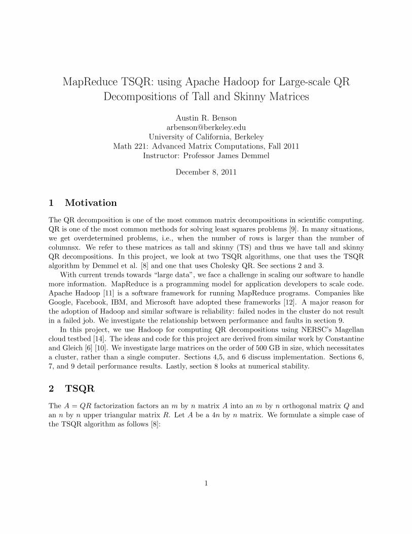
The A = QR factorization factors an m by n matrix A into an m by n orthogonal matrix Q andan n by n upper triangular matrix R. Let A be a 4n by n matrix. We formulate a simple case ofthe TSQR algorithm as follows [8]:

1

A =

A1

A2

A3

A4

=

Q1R1

Q2R2

Q3R3

Q4R4

→

R1

R2

R3

R4

=

�Q5R5

Q6R6

�→

�R5

R6

�= Q7R7. (1)

Each intermediate QiRi factorization is a local factorization. Ai and Qi are n by n for i =1, 2, 3, 4, Qi is 2n by n for i = 5, 6 and Q7 is 4n by n. Ri is n by n for i = 1, 2, ..., 7. The QRdecomposition is given by A = QR7, where Q is constructed from the Qi by equation 2:

Q =

Q1

Q2

Q3

Q4

�Q5

Q6

�Q7 (2)

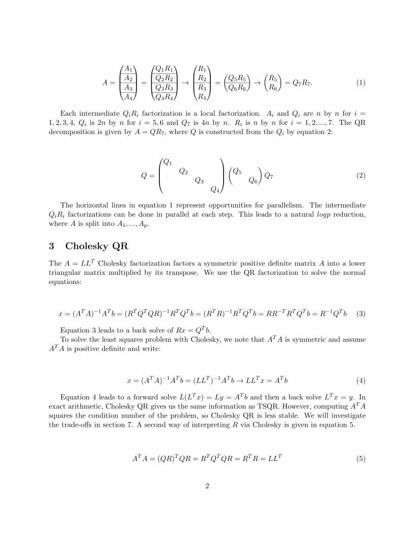
The horizontal lines in equation 1 represent opportunities for parallelism. The intermediateQiRi factorizations can be done in parallel at each step. This leads to a natural logp reduction,where A is split into A1, ..., Ap.

3 Cholesky QR

The A = LLT Cholesky factorization factors a symmetric positive definite matrix A into a lowertriangular matrix multiplied by its transpose. We use the QR factorization to solve the normalequations:

x = (ATA)−1AT b = (RTQTQR)−1RTQT b = (RTR)−1RTQT b = RR−TRTQT b = R−1QT b (3)

Equation 3 leads to a back solve of Rx = QT b.To solve the least squares problem with Cholesky, we note that ATA is symmetric and assume

ATA is positive definite and write:

x = (ATA)−1AT b = (LLT )−1AT b → LLTx = AT b (4)

Equation 4 leads to a forward solve L(LTx) = Ly = AT b and then a back solve LTx = y. Inexact arithmetic, Cholesky QR gives us the same information as TSQR. However, computing ATAsquares the condition number of the problem, so Cholesky QR is less stable. We will investigatethe trade-offs in section 7. A second way of interpreting R via Cholesky is given in equation 5.

ATA = (QR)TQR = RTQTQR = RTR = LLT (5)

2

4 Applying the MapReduce model to QR

In general, the Map Reduce model follows an iterative three-step process using key-value pairs.Let ki and vi represent keys and values, respectively, for i = 1, 2, 3. Then we can represent thethree-step process by the composition of three functions:

(k1, v1)map−−→ (k2, v2)

combine−−−−−→ (k2, v2)reduce−−−−→ (k3, v3)

For simplicity, we will ignore the combine step and only consider the map and reduce steps:

(k1, v1)map−−→ (k2, v2)

reduce−−−−→ (k3, v3)

v2 is treated as a list of values emitted by the map function all corresponding to a given key.We will use the following notation to indicate how many map and reduce tasks are used in a giveniteration:

(k1, v1)map−−→nm

(k2, v2)reduce−−−−→nr

(k3, v3) (6)

Equation 6 indicates that there are nm map tasks and nr reduce tasks. We will let max indicatethat the maximum available tasks will be used.

We will denote the MapReduce model for TSQR and Cholesky QR by MRTSQR and MRCQR,respectively.

4.1 MRTSQR

The parallelism for TSQR is evident in the parallel local QR decompositions in section 2. MRTSQRuses both the map and reduce steps to perform local QR decompositions on leftover intermediateRi. The functions look like:

(k,Ai)QR−−→ (k,Ri)

QR−−→ (k,Ri).

Each map and reduce task outputs one intermediate Ri. In order to combine the results fromthe distributed reduce tasks, we introduce a second iteration:

(k,Ai)QR−−−→max

(k,Ri)QR−−−→max

(k,Ri)identity−−−−−→max

(k,Ri)QR−−→1

(i, R). (7)

A visual interpretation of equation 7 is given in Figure 1.

3

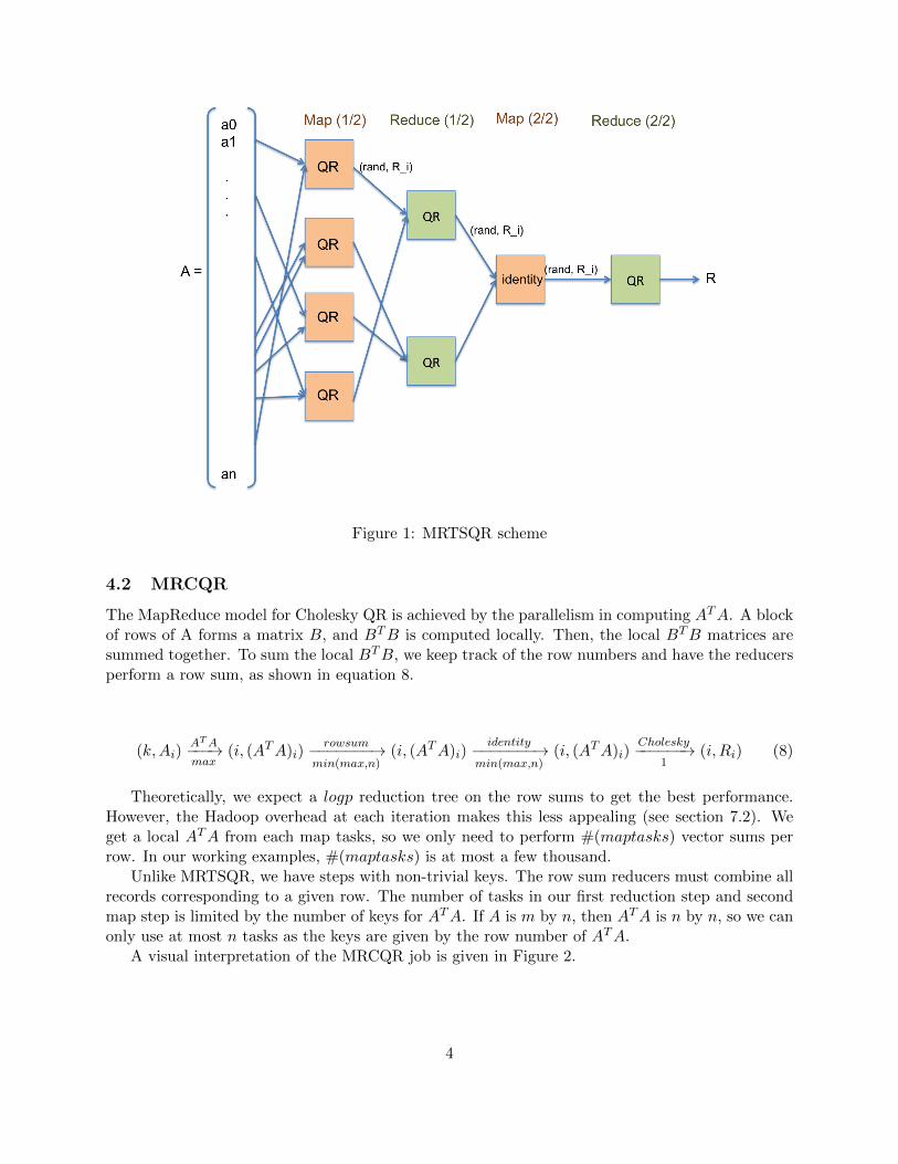
Figure 1: MRTSQR scheme

4.2 MRCQR

The MapReduce model for Cholesky QR is achieved by the parallelism in computing ATA. A blockof rows of A forms a matrix B, and BTB is computed locally. Then, the local BTB matrices aresummed together. To sum the local BTB, we keep track of the row numbers and have the reducersperform a row sum, as shown in equation 8.

(k,Ai)ATA−−−→max

(i, (ATA)i)rowsum−−−−−−−→

min(max,n)(i, (ATA)i)

identity−−−−−−−→min(max,n)

(i, (ATA)i)Cholesky−−−−−−→

1(i, Ri) (8)

Theoretically, we expect a logp reduction tree on the row sums to get the best performance.However, the Hadoop overhead at each iteration makes this less appealing (see section 7.2). Weget a local ATA from each map tasks, so we only need to perform #(maptasks) vector sums perrow. In our working examples, #(maptasks) is at most a few thousand.

Unlike MRTSQR, we have steps with non-trivial keys. The row sum reducers must combine allrecords corresponding to a given row. The number of tasks in our first reduction step and secondmap step is limited by the number of keys for ATA. If A is m by n, then ATA is n by n, so we canonly use at most n tasks as the keys are given by the row number of ATA.

A visual interpretation of the MRCQR job is given in Figure 2.

4

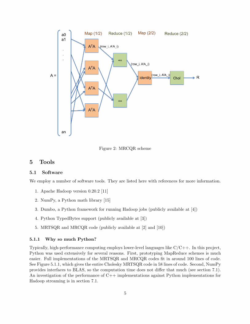
Figure 2: MRCQR scheme

5 Tools

5.1 Software

We employ a number of software tools. They are listed here with references for more information.

1. Apache Hadoop version 0.20.2 [11]

2. NumPy, a Python math library [15]

3. Dumbo, a Python framework for running Hadoop jobs (publicly available at [4])

4. Python TypedBytes support (publicly available at [3])

5. MRTSQR and MRCQR code (publicly available at [2] and [10])

5.1.1 Why so much Python?

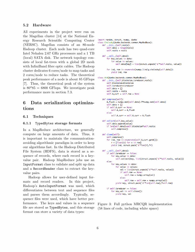
Typically, high-performance computing employs lower-level languages like C/C++. In this project,Python was used extensively for several reasons. First, prototyping MapReduce schemes is mucheasier. Full implementations of the MRTSQR and MRCQR codes fit in around 100 lines of code.See Figure 5.1.1, which gives the entire Cholesky MRTSQR code in 58 lines of code. Second, NumPyprovides interfaces to BLAS, so the computation time does not differ that much (see section 7.1).An investigation of the performance of C++ implementations against Python implementations forHadoop streaming is in section 7.1.

5

5.2 Hardware

Figure 3: Full python MRCQR implementation(58 lines of code, including white space)

All experiments in the project were run onthe Magellan cluster [14] at the National En-ergy Research Scientific Computing Center(NERSC). Magellan consists of an 80-nodeHadoop cluster. Each node has two quad-coreIntel Nehalen 2.67 GHz processors and a 1 TB(local) SATA disk. The network topology con-sists of local fat-trees with a global 2D meshwith InfiniBand fibre optic cables. The Hadoopcluster dedicates 6 cores/node to map tasks and2 cores/node to reduce tasks. The theoreticalpeak performance of a node is about 85 GFlops[7]. Thus, the theoretical peak of the systemis 80*85 = 6800 GFlops. We investigate peakperformance more in section 7.3.

6 Data serialization optimiza-

tions

6.1 Techniques

6.1.1 TypedBytes storage formats

In a MapReduce architecture, we generallycompute on large amounts of data. Thus, itis important to maintain the communication-avoiding algorithmic paradigm in order to keepour algorithms fast. In the Hadoop DistributedFile System (HDFS), data is stored as a se-quence of records, where each record is a key-value pair. Hadoop MapReduce jobs use anInputFormat class to validate and split up dataand a RecordReader class to extract the key-value pairs.

Hadoop allows for user-defined input for-mats and record readers. In this project,Hadoop’s AutoInputFormat was used, whichdifferentiates between text and sequence filesand parses them accordingly. Typically, se-quence files were used, which have better per-formance. The keys and values in a sequencefile are stored as TypedBytes, and this storageformat can store a variety of data types:

6

(a) TypedBytes List (b) TypedBytes String

Figure 4: Simplified models of TypedBytes data structures

• Fixed-length data types: Byte, Bool, Int,Long, Float, Double

• Variable-length data types: Bytes, String,Vector, List

In this project, we evaluated performance differences from these data types. The originalimplementation by Constantine and Gleich [6] uses a TypedBytes List format, which maintains thelist structure in the record. In order to reduce the amount of metadata moved by Hadoop jobs, aTypedBytes String format was used. The python struct module allows for reading and writingthis data type (see [2], [10] for implementation details). Figure 4 illustrates the difference betweena TypedBytes List and TypedBytes String. See section 6.2 for performance results.

6.1.2 Row packing

The second type of data serialization used is row packing. Typically, we store the matrix with onerow per record. For very skinny matrices, it can be beneficial to store multiple rows in one record.For the experiments in section 6.2, we look at matrices with 4, 10, and 200 rows.

6.2 Experiments and Performance

Experiments were performed on three different matrices: (1) 20 billion by 4 (∼600 GB), (2) 800million by 10 (∼60 GB), (3) 200 million by 200 (∼300 GB). Tests were performed 5 times, repre-sented by the x-axis as trials in Figures 5, 6, and 7. We expect that each matrix will benefit fromthe TypedBytes String format. We also expect that matrices with a smaller number of columns willbenefit more from packed rows. These experiments were performed with the MRTSQR algorithm.

All three matrices benefited extraordinarily from the switch from a TypedBytes List to a Type-dBytes String storage format. Speedups from this optimization were approximately 1.7-2x. Packedrows also resulted in significant speedups. With the 20 billion by 4 matrix, packing two rows perrecord resulted in an additional 20% performance increase, and packing four rows per record re-sulted in another additional 20%. With the 800 million by 10 matrix, we see that packing two rowper record increased performance, but packing four rows per record resulted in erratic performance.With the 200 million by 2 matrix, packing two rows per record left the performance approximatelyunchanged.

7

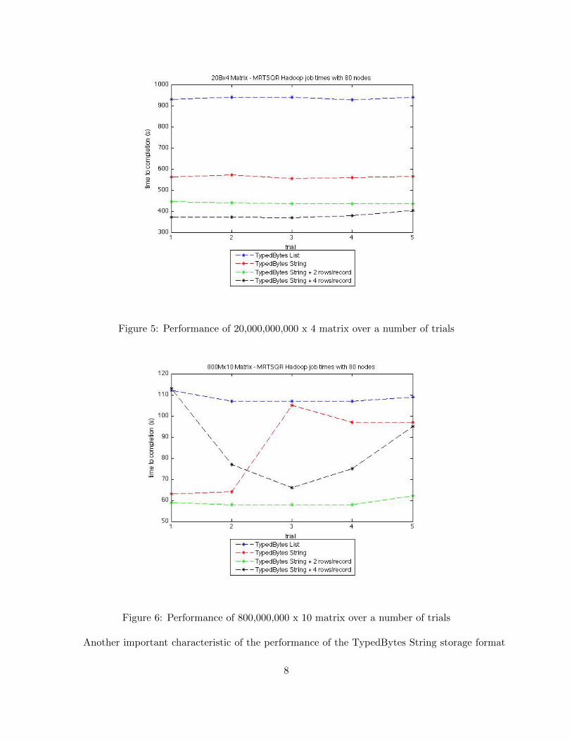
Figure 5: Performance of 20,000,000,000 x 4 matrix over a number of trials

Figure 6: Performance of 800,000,000 x 10 matrix over a number of trials

Another important characteristic of the performance of the TypedBytes String storage format

8

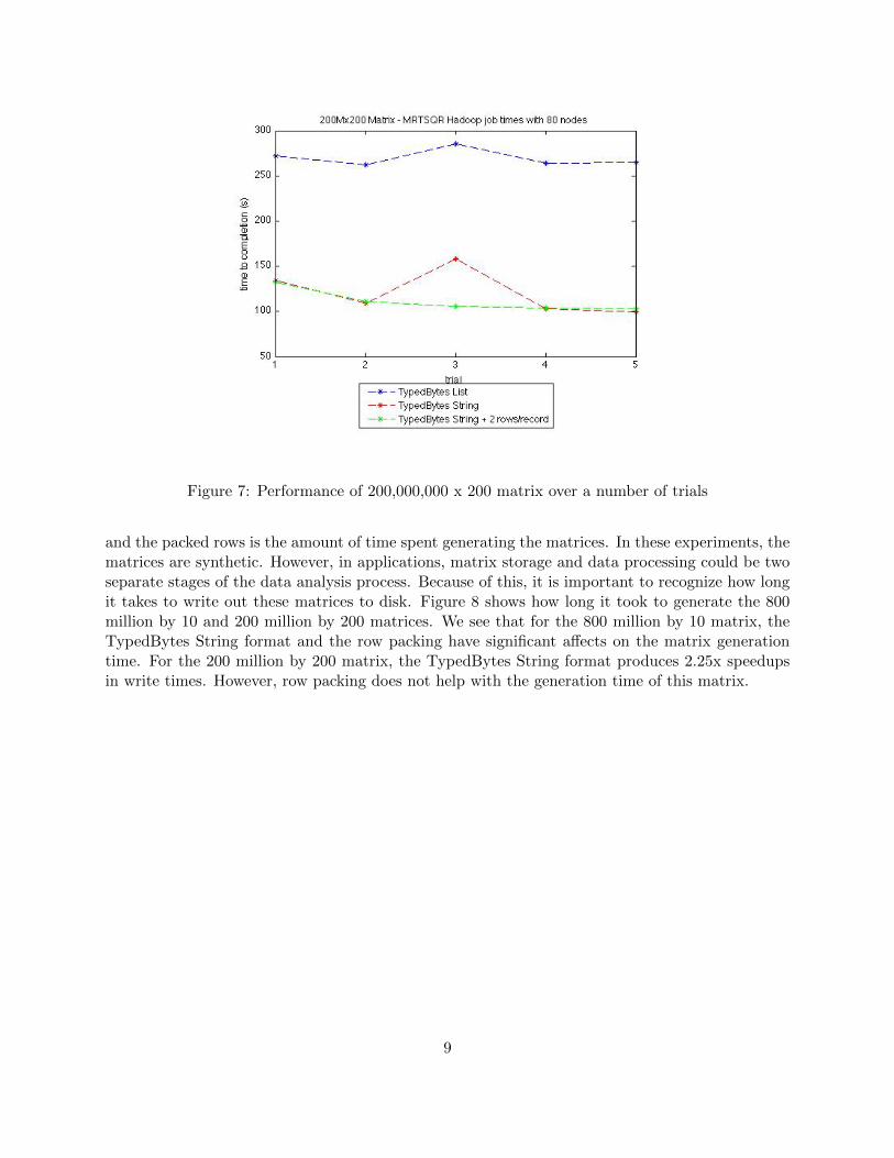
Figure 7: Performance of 200,000,000 x 200 matrix over a number of trials

and the packed rows is the amount of time spent generating the matrices. In these experiments, thematrices are synthetic. However, in applications, matrix storage and data processing could be twoseparate stages of the data analysis process. Because of this, it is important to recognize how longit takes to write out these matrices to disk. Figure 8 shows how long it took to generate the 800million by 10 and 200 million by 200 matrices. We see that for the 800 million by 10 matrix, theTypedBytes String format and the row packing have significant affects on the matrix generationtime. For the 200 million by 200 matrix, the TypedBytes String format produces 2.25x speedupsin write times. However, row packing does not help with the generation time of this matrix.

9

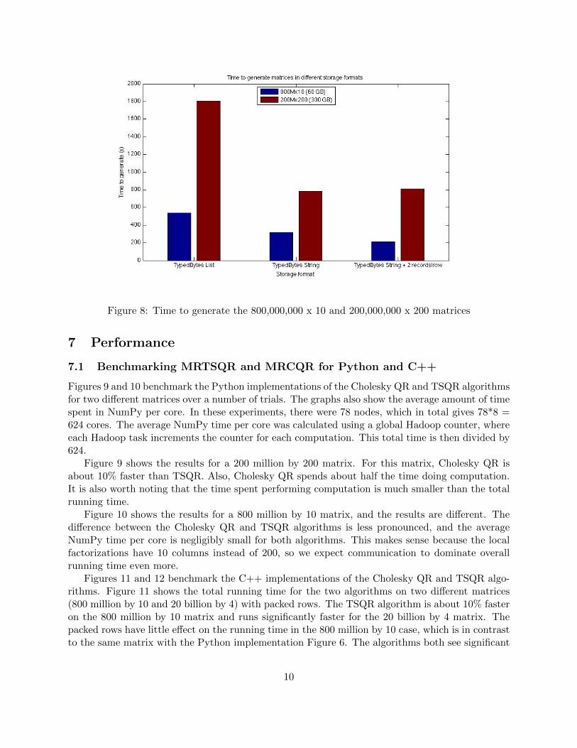
Figure 8: Time to generate the 800,000,000 x 10 and 200,000,000 x 200 matrices

7 Performance

7.1 Benchmarking MRTSQR and MRCQR for Python and C++

Figures 9 and 10 benchmark the Python implementations of the Cholesky QR and TSQR algorithmsfor two different matrices over a number of trials. The graphs also show the average amount of timespent in NumPy per core. In these experiments, there were 78 nodes, which in total gives 78*8 =624 cores. The average NumPy time per core was calculated using a global Hadoop counter, whereeach Hadoop task increments the counter for each computation. This total time is then divided by624.

Figure 9 shows the results for a 200 million by 200 matrix. For this matrix, Cholesky QR isabout 10% faster than TSQR. Also, Cholesky QR spends about half the time doing computation.It is also worth noting that the time spent performing computation is much smaller than the totalrunning time.

Figure 10 shows the results for a 800 million by 10 matrix, and the results are different. Thedifference between the Cholesky QR and TSQR algorithms is less pronounced, and the averageNumPy time per core is negligibly small for both algorithms. This makes sense because the localfactorizations have 10 columns instead of 200, so we expect communication to dominate overallrunning time even more.

Figures 11 and 12 benchmark the C++ implementations of the Cholesky QR and TSQR algo-rithms. Figure 11 shows the total running time for the two algorithms on two different matrices(800 million by 10 and 20 billion by 4) with packed rows. The TSQR algorithm is about 10% fasteron the 800 million by 10 matrix and runs significantly faster for the 20 billion by 4 matrix. Thepacked rows have little effect on the running time in the 800 million by 10 case, which is in contrastto the same matrix with the Python implementation Figure 6. The algorithms both see significant

10

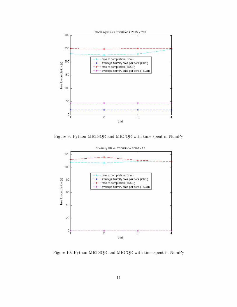
Figure 9: Python MRTSQR and MRCQR with time spent in NumPy

Figure 10: Python MRTSQR and MRCQR with time spent in NumPy

11

speedups due to the packed rows of the 20 billion by 4 matrix.Figure 12 looks at the average LAPACK time per core, i.e. the amount of time spent in

computation per core. Interestingly, the TSQR algorithm spends less time in computation than theCholesky QR algorithm. However, we also see variations in the computation time across differentpacked rows. Note that the average time spent in LAPACK per core is less than 0.1 seconds inall cases, so variations could be due to errors in timing, or function call overhead. The CholeskyQR algorithm makes several thousand more calls to LAPACK. The algorithm calls dsyrk for ATA,daxpy for row sums, and dpotrf for Cholesky. TSQR only makes calls to dgeqrf.

Figure 11: C++ MRTSQR and MRCQR total job times

12

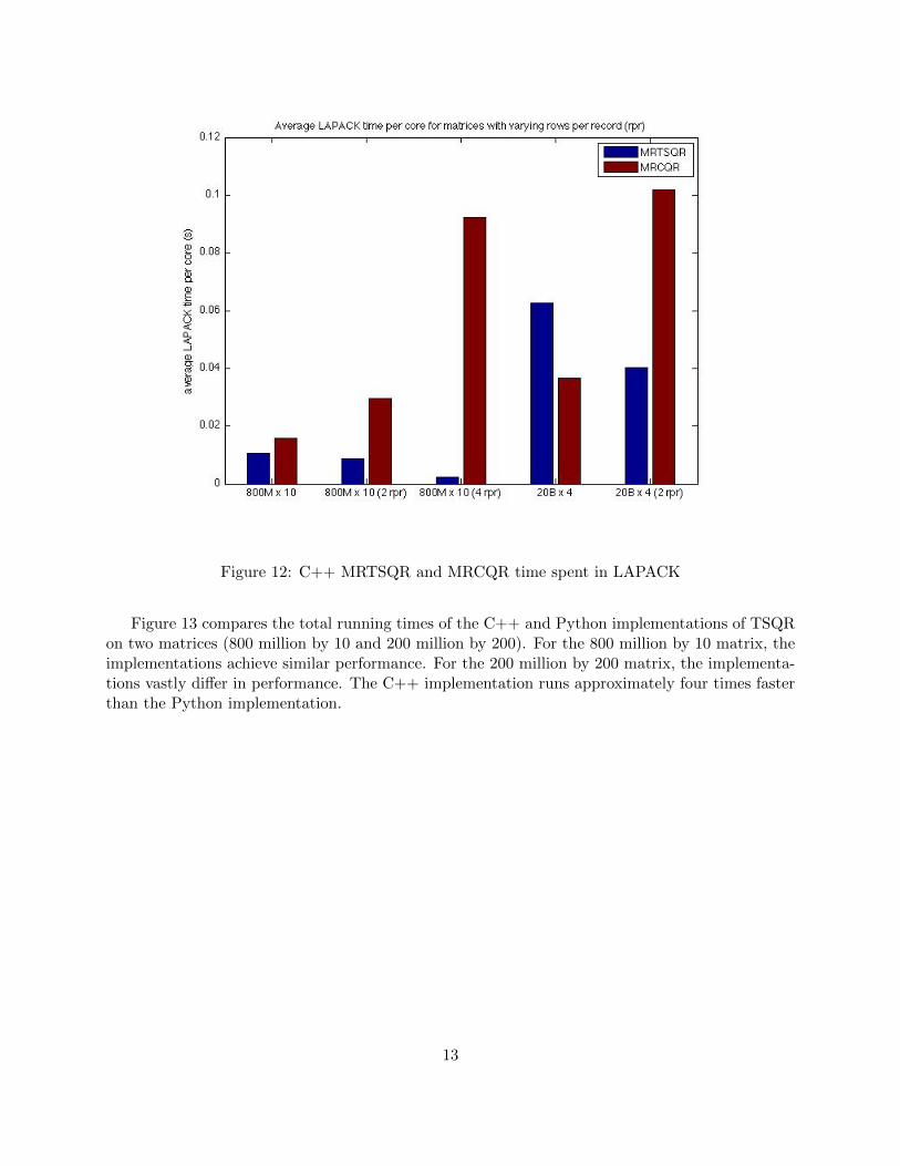
Figure 12: C++ MRTSQR and MRCQR time spent in LAPACK

Figure 13 compares the total running times of the C++ and Python implementations of TSQRon two matrices (800 million by 10 and 200 million by 200). For the 800 million by 10 matrix, theimplementations achieve similar performance. For the 200 million by 200 matrix, the implementa-tions vastly differ in performance. The C++ implementation runs approximately four times fasterthan the Python implementation.

13

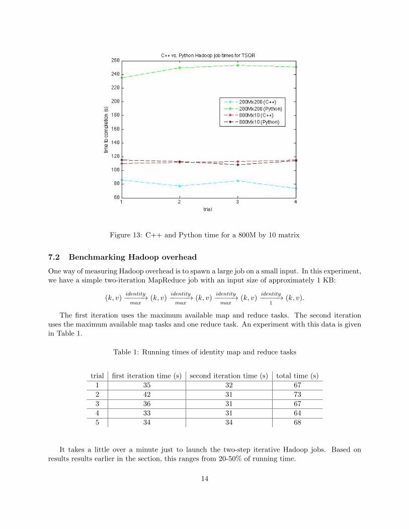
Figure 13: C++ and Python time for a 800M by 10 matrix

7.2 Benchmarking Hadoop overhead

One way of measuring Hadoop overhead is to spawn a large job on a small input. In this experiment,we have a simple two-iteration MapReduce job with an input size of approximately 1 KB:

(k, v)identity−−−−−→max

(k, v)identity−−−−−→max

(k, v)identity−−−−−→max

(k, v)identity−−−−−→

1(k, v).

The first iteration uses the maximum available map and reduce tasks. The second iterationuses the maximum available map tasks and one reduce task. An experiment with this data is givenin Table 1.

Table 1: Running times of identity map and reduce tasks

trial first iteration time (s) second iteration time (s) total time (s)1 35 32 672 42 31 733 36 31 674 33 31 645 34 34 68

It takes a little over a minute just to launch the two-step iterative Hadoop jobs. Based onresults results earlier in the section, this ranges from 20-50% of running time.

14

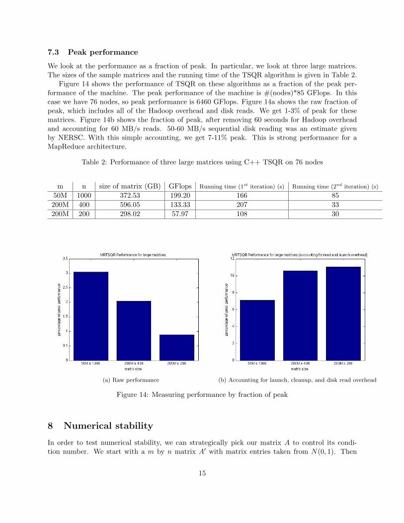
7.3 Peak performance

We look at the performance as a fraction of peak. In particular, we look at three large matrices.The sizes of the sample matrices and the running time of the TSQR algorithm is given in Table 2.

Figure 14 shows the performance of TSQR on these algorithms as a fraction of the peak per-formance of the machine. The peak performance of the machine is #(nodes)*85 GFlops. In thiscase we have 76 nodes, so peak performance is 6460 GFlops. Figure 14a shows the raw fraction ofpeak, which includes all of the Hadoop overhead and disk reads. We get 1-3% of peak for thesematrices. Figure 14b shows the fraction of peak, after removing 60 seconds for Hadoop overheadand accounting for 60 MB/s reads. 50-60 MB/s sequential disk reading was an estimate givenby NERSC. With this simple accounting, we get 7-11% peak. This is strong performance for aMapReduce architecture.

Table 2: Performance of three large matrices using C++ TSQR on 76 nodes

m n size of matrix (GB) GFlops Running time (1st iteration) (s) Running time (2nd iteration) (s)

50M 1000 372.53 199.20 166 85200M 400 596.05 133.33 207 33200M 200 298.02 57.97 108 30

(a) Raw performance (b) Accounting for launch, cleanup, and disk read overhead

Figure 14: Measuring performance by fraction of peak

8 Numerical stability

In order to test numerical stability, we can strategically pick our matrix A to control its condi-tion number. We start with a m by n matrix A� with matrix entries taken from N(0, 1). Then

15

we compute A� = Q�R�. Q� also has matrix entries from N(0, 1). Let D be a diagonal matrixwith Djj > 0. We then take a n by n matrix A with matrix entries from N(0, 1) and computeA = QR. Finally, let A = Q�DQ. This is precisely the SVD of A, so we get the condition number by:

κ(A) =σmax

σmin=

maxj Djj

minj Djj[9].

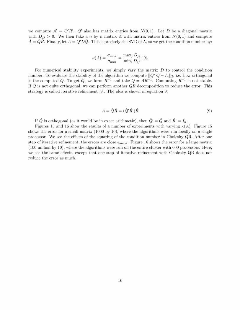
For numerical stability experiments, we simply vary the matrix D to control the conditionnumber. To evaluate the stability of the algorithm we compute ||QTQ− In||2, i.e. how orthogonalis the computed Q. To get Q, we form R−1 and take Q = AR−1. Computing R−1 is not stable.If Q is not quite orthogonal, we can perform another QR decomposition to reduce the error. Thisstrategy is called iterative refinement [9]. The idea is shown in equation 9:

A = QR = (Q�R�)R (9)

If Q is orthogonal (as it would be in exact arithmetic), then Q� = Q and R� = In.Figures 15 and 16 show the results of a number of experiments with varying κ(A). Figure 15

shows the error for a small matrix (1000 by 10), where the algorithms were run locally on a singleprocessor. We see the effects of the squaring of the condition number in Cholesky QR. After onestep of iterative refinement, the errors are close �mach. Figure 16 shows the error for a large matrix(100 million by 10), where the algorithms were run on the entire cluster with 600 processors. Here,we see the same effects, except that one step of iterative refinement with Cholesky QR does notreduce the error as much.

16

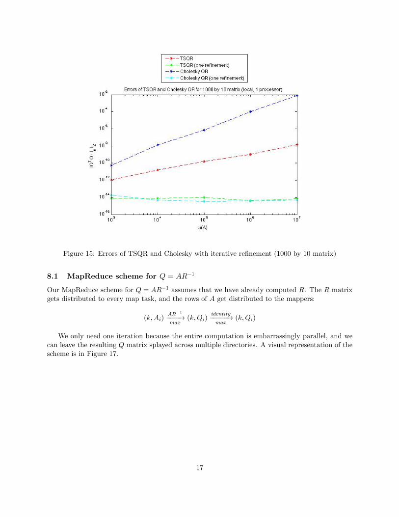
Figure 15: Errors of TSQR and Cholesky with iterative refinement (1000 by 10 matrix)

8.1 MapReduce scheme for Q = AR−1

Our MapReduce scheme for Q = AR−1 assumes that we have already computed R. The R matrixgets distributed to every map task, and the rows of A get distributed to the mappers:

(k,Ai)AR−1

−−−−→max

(k,Qi)identity−−−−−→max

(k,Qi)

We only need one iteration because the entire computation is embarrassingly parallel, and wecan leave the resulting Q matrix splayed across multiple directories. A visual representation of thescheme is in Figure 17.

17

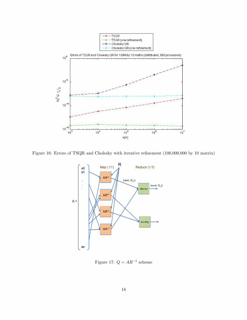
Figure 16: Errors of TSQR and Cholesky with iterative refinement (100,000,000 by 10 matrix)

Figure 17: Q = AR−1 scheme

18

9 Fault tolerance

The central benefit to scientific computing in cloud environments is stability. In Hadoop, failedtasks are restarted 3 times by default, and this is a tunable parameter [11]. This provides the userwith the comfort that a single point of failure will not derail entire jobs. Furthermore, consistentlyfailing nodes are “blacklisted” and not included in future jobs.

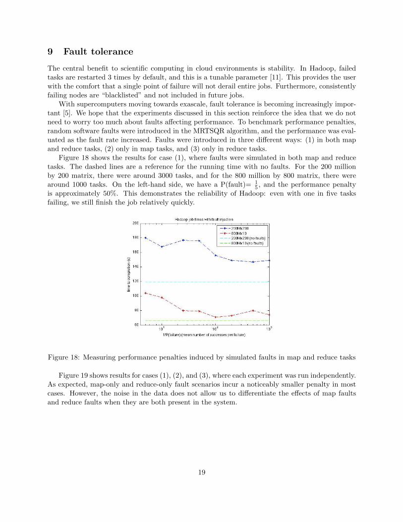
With supercomputers moving towards exascale, fault tolerance is becoming increasingly impor-tant [5]. We hope that the experiments discussed in this section reinforce the idea that we do notneed to worry too much about faults affecting performance. To benchmark performance penalties,random software faults were introduced in the MRTSQR algorithm, and the performance was eval-uated as the fault rate increased. Faults were introduced in three different ways: (1) in both mapand reduce tasks, (2) only in map tasks, and (3) only in reduce tasks.

Figure 18 shows the results for case (1), where faults were simulated in both map and reducetasks. The dashed lines are a reference for the running time with no faults. For the 200 millionby 200 matrix, there were around 3000 tasks, and for the 800 million by 800 matrix, there werearound 1000 tasks. On the left-hand side, we have a P(fault)= 1

5 , and the performance penaltyis approximately 50%. This demonstrates the reliability of Hadoop: even with one in five tasksfailing, we still finish the job relatively quickly.

Figure 18: Measuring performance penalties induced by simulated faults in map and reduce tasks

Figure 19 shows results for cases (1), (2), and (3), where each experiment was run independently.As expected, map-only and reduce-only fault scenarios incur a noticeably smaller penalty in mostcases. However, the noise in the data does not allow us to differentiate the effects of map faultsand reduce faults when they are both present in the system.

19

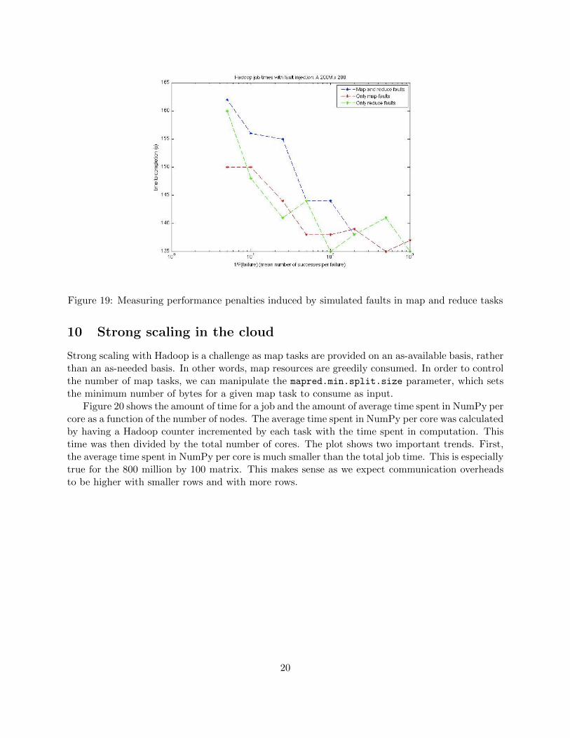
Figure 19: Measuring performance penalties induced by simulated faults in map and reduce tasks

10 Strong scaling in the cloud

Strong scaling with Hadoop is a challenge as map tasks are provided on an as-available basis, ratherthan an as-needed basis. In other words, map resources are greedily consumed. In order to controlthe number of map tasks, we can manipulate the mapred.min.split.size parameter, which setsthe minimum number of bytes for a given map task to consume as input.

Figure 20 shows the amount of time for a job and the amount of average time spent in NumPy percore as a function of the number of nodes. The average time spent in NumPy per core was calculatedby having a Hadoop counter incremented by each task with the time spent in computation. Thistime was then divided by the total number of cores. The plot shows two important trends. First,the average time spent in NumPy per core is much smaller than the total job time. This is especiallytrue for the 800 million by 100 matrix. This makes sense as we expect communication overheadsto be higher with smaller rows and with more rows.

20

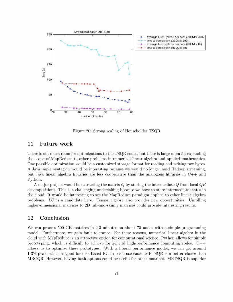
Figure 20: Strong scaling of Householder TSQR

11 Future work

There is not much room for optimizations to the TSQR codes, but there is large room for expandingthe scope of MapReduce to other problems in numerical linear algebra and applied mathematics.One possible optimization would be a customized storage format for reading and writing raw bytes.A Java implementation would be interesting because we would no longer need Hadoop streaming,but Java linear algebra libraries are less cooperative than the analogous libraries in C++ andPython.

A major project would be extracting the matrix Q by storing the intermediate Q from local QRdecompositions. This is a challenging undertaking because we have to store intermediate states inthe cloud. It would be interesting to see the MapReduce paradigm applied to other linear algebraproblems. LU is a candidate here. Tensor algebra also provides new opportunities. Unrollinghigher-dimensional matrices to 2D tall-and-skinny matrices could provide interesting results.

12 Conclusion

We can process 500 GB matrices in 2-3 minutes on about 75 nodes with a simple programmingmodel. Furthermore, we gain fault tolerance. For these reasons, numerical linear algebra in thecloud with MapReduce is an attractive option for computational science. Python allows for simpleprototyping, which is difficult to achieve for general high-performance computing codes. C++allows us to optimize these prototypes. With a liberal performance model, we can get around1-3% peak, which is good for disk-based IO. In basic use cases, MRTSQR is a better choice thanMRCQR. However, having both options could be useful for other matrices. MRTSQR is superior

21

in terms of numerical stability, as expected.

13 Acknowledgements

Thanks to Professor David Gleich for project ideas, software help, and answering numerous ques-tions. Thanks to Professor Jim Demmel for teaching the course and for project ideas. Thanks toGrey Ballard for being the course GSI and for answering questions in office hours. Lastly, thanks tothe NERSC team (in particular, Lavanya Ramakrishnan and Iwona Sakrejda) for answering severalquestions.

References

[1] The Apache Software Foundation. MapReduce Tutorial. 2008.

� http://hadoop.apache.org/common/docs/current/mapred tutorial.html �

[2] Austin Benson. MapReduce TSQR code. � https://github.com/arbenson/mrtsqr �

[3] Klaas Bosteels. TypedBytes. � https://github.com/klbostee/typedbytes �

[4] Klaas Bosteels. Dumbo. � https://github.com/klbostee/dumbo �

[5] Franck Cappello. Fault Tolerance in Petascale/Exascale Systems: Current Knowledge, Chal-lenges and Research Opportunities. The International Journal of High Performance Computing

Applications 23.3, (2009): 212–222.

[6] Paul G. Constantine and David F. Gleich. Tall and skinny QR factorizations in MapReducearchitectures. In Proceedings of the second international workshop on MapReduce and its ap-

plications, MapReduce ’11, pages 43-50, New York, NY, USA, 2011. ACM.

[7] Shane Corder. High Performance Linpack on Xeon 5500 v. Opteron 2400. 16June 2009. � http://www.advancedclustering.com/company-blog/high-performance-linpack-on-xeon-5500-v-opteron-2400.html �. Accessed 11 November 2011.

[8] James Demmel, Laura Grigori, Mark F. Hoemmen, and Julien Langou. Communication-optimal parallel and sequential QR and LU factorizations. UCB/EECS-2008-89. August 2008.

[9] James Demmel. Applied Numerical Linear Algebra. SIAM. 1997.

[10] David Gleich. MapReduce TSQR code. � https://github.com/dgleich/mrtsqr �

[11] Hadoop version 0.20. � http://hadoop.apache.org/ �

[12] Hadoop Wiki: PoweredBy. � http://wiki.apache.org/hadoop/PoweredBy �

[13] Herodotos Herodotou. Hadoop Performance Models. Technical Report, CS-2011-05. Duke Uni-versity. May 2011.

[14] Magellan at NERSC. � http://magellan.nersc.gov �

[15] Eric Jones, Travis Oliphant, Pearu Peterson and others. SciPy: Open Source Scientific Toolsfor Python. 2001. � http://www.scipy.org �

22