Mapping Land Use Systems at global and regional scales for
70
LADA LANDDEGRADATION ASSESSMENTIN DRYLANDS MAPPING LAND USE SYSTEMS AT GLOBAL AND REGIONAL SCALES FOR LAND DEGRADATION ASSESSMENT ANALYSIS Version 1.1 LADA PROJECT
Transcript of Mapping Land Use Systems at global and regional scales for

LADA
LANDDEGRADATIONASSESSMENTIN DRYLANDS
MAPPING LAND USE SYSTEMS AT GLOBAL AND REGIONAL SCALES FOR LAND DEGRADATION ASSESSMENT ANALYSIS
Version 1.1
LADAP R O J E C T

Cover photos:above: Ch. Errathbelow: LADA project
Cover design:Simone Morini

FOOD AND AGRICULTURE ORGANIZATION OF THE UNITED NATIONSRome, 2013
LANDDEGRADATIONASSESSMENTIN DRYLANDS
general coordinatorsFreddy Nachtergaele and Riccardo Biancalani
FAO, Rome, Italy
authorsFreddy Nachtergaele
Monica Petri
editorAnne Woodfine
MAPPING LAND USE SYSTEMS AT GLOBAL AND REGIONALSCALES FOR LAND DEGRADATION ASSESSMENT ANALYSIS
Version 1.1

This work was originally published online by the Food and Agriculture Organization of the United Nations in 2011.
The designations employed and the presentation of material in this information product do not imply the expression of any opinion whatsoever on the part of the Food and Agriculture Organization of the United Nations (FAO) concerning the legal or development status of any country, territory, city or area or of its authorities, or concerning the delimitation of its frontiers or boundaries. The mention of specific companies or products of manufacturers, whether or not these have been patented, does not imply that these have been endorsed or recommended by FAO in preference to others of a similar nature that are not mentioned.
The views expressed in this information product are those of the author(s) and do not necessarily reflect the views or policies of FAO.
ISBN 978-92-5-107568-5 (print)E-ISBN 978-92-5-107569-2 (PDF)
© FAO 2011, 2013
FAO encourages the use, reproduction and dissemination of material in this information product. Except where otherwise indicated, material may be copied, downloaded and printed for private study, research and teaching purposes, or for use in non-commercial products or services, provided that appropriate acknowledgement of FAO as the source and copyright holder is given and that FAO’s endorsement of users’ views, products or services is not implied in any way.
All requests for translation and adaptation rights, and for resale and other commercial use rights should be made via www.fao.org/contact-us/licence-request or addressed to [email protected].
FAO information products are available on the FAO website (www.fao.org/publications) and can be purchased through [email protected].

CO
NTE
NTS
Acknowledgements v
Acronyms and abbreviations vi
1 Introduction 11.1 Land Degradation Assessment in Drylands project
and Land Use Systems 11.2 The ecosystem-Land Use System information base 21.3 Base data and data quality 81.4 From a global to a national Land Use Systems map 9
2 Global Ecosystems and Land Use Systems 112.1 Land cover 122.2 Irrigation 122.3 Urban areas 132.4 Protected areas 142.5 Presence of livestock in the Land Use Systems 142.6 Forest use in the Land Use Systems 152.7 Technical procedure to obtain the major Land Use Systems 15
3 The major ecosystems 173.1 Global base maps used 173.2 Procedure 18
4 The land use attributes 214.1 Dominant livestock types 214.2 Dominant crop types 214.3 Small-scale irrigation 224.4 Crop management index 22
5 Biophysical attributes of ecosystems 235.1 Temperature regime class 235.2 Length of growing period class 235.3 Dominant soil unit 235.4 Terrain information 24
6 Socio-economic attributes of Land Use Systems 256.1 Population density 256.2 Poverty 26
iv LAND DEGRADATION ASSESSMENT IN DRYLANDS (LADA) PROJECT
Annexes1 Input and output maps in Land Use Systems method 272 Livestock presence in Land Use Systems 413 Dominant crop type in Land Use Systems 494 Technical specifications 55
References 75

Acknowledgements
vLAND DEGRADATION ASSESSMENT IN DRYLANDS (LADA) PROJECT
This report draws heavily on the earlier work of John Dixon, Hubert George and others who made considerable progress in improving the sub-national land use information in FAO and whose intellectual efforts in this field are herewith gratefully acknowledged. The work would have been impossible without the ongoing work in various sections of FAO that improved the individual databases used – in particular: John Latham (land cover and poverty); Tim Robinson and Gianluca Franceschini (livestock). Support, suggestions and comments received from Dominique Lantieri, Leslie Lipper and other members of the Stratification Task Force is also gratefully acknowledged. The report has benefited enormously from comments and suggestions received from the national LADA coordinators and their collaborators – in particular; Dirk Pretorius, Dethie Ndiaye, Jia Xiaoxia, Michael Laker, Andres Ravelo and Hedi Hamrouni, who are especially thanked for their constructive criticism of earlier versions.

Acronyms and abbreviations
CIESIN Centre for International Earth Science Information Network CRU Climate Research Unit (of the University of East Anglia)
DPSIR Drivers-Pressure-State-Impact-ResponseFAO Food and Agriculture Organization of the United Nations
GPCC Global Precipitation Climatology Centre GRUMP Global Rural Urban Mapping Programme
IUCN International Union for the Conservation of NatureLADA Land Degradation Assessment in Drylands
LGP length of growing periodLUS land use system
MDG Millennium Development GoalN-LUS national-land use system
PET potential evapotranspirationSLM sustainable land management
TLU tropical livestock unitUNEP United Nations Environment Programme
UNESCO-MAP United Nations Educational, Scientific and Cultural Organization– Man and the Biosphere Programme
WCMC World Conservation Monitoring CentreWOCAT World Overview of Conservation Approaches and Technologies
vi LAND DEGRADATION ASSESSMENT IN DRYLANDS (LADA) PROJECT

Introduction
CH
APT
ER1
1.1 Land Degradation Assessment in Drylands projectand Land Use Systems
The objective of the Land Degradation Assessment in Drylands (LADA) project was to develop tools and methods to assess and quantify the nature, extent, severity and impacts of land degradation on dryland ecosystems, watersheds and river basins, carbon storage and biological diversity at a range of spatial and temporal scales. This builds the national, regional and international capacity to analyze, design, plan and implement interventions to mitigate land degradation and establish sustainable land use and management practices.
To achieve this objective, LADA has developed standardized and improved methods for dryland degradation assessment, with guidelines for their implementation at a range of spatial and / or temporal scales. The LADA methods enable users to assess the regional and global baseline land degradation situation with the view to highlighting the areas at greatest risk. These assessments were supplemented by detailed local assessments that focused on the root causes of land degradation and on local (traditional and adapted) technologies for the mitigation of land degradation. Areas where land degradation is well controlled were included in the analysis in order to develop ‘best practice’ guidelines and the results widely disseminated in various media. The project was intended to make an innovative generic contribution to methodologies and monitoring systems for land degradation, supplemented by empirically-derived lessons from the six main partner countries involved in Phase 1 of the project (Argentina, China, Cuba, Senegal, South Africa and Tunisia) for up-scaling to countries within their regional remit.

MAPPING LAND USE SYSTEMS AT GLOBAL AND REGIONAL SCALES FOR LAND DEGRADATION ASSESSMENT ANALYSISVersion 1.1
2 LAND DEGRADATION ASSESSMENT IN DRYLANDS (LADA) PROJECT
Land degradation can be defined as a long term loss of ecosystem functions over time, as perceived by the land users. The relationship between land degradation and land use is clear, as land use implicitly includes the way farmers and pastoralists use and manage the land, which can inherently change it for the better and / or the worse. Knowledge of local biophysical and socio-economic conditions is needed to explain and relate the land use to land degradation and vice versa. The methodology presented here describes the principles to map land use and inventory related ecosystems and more detailed crop or livestock information at a global scale. Refinements of this methodology are required when applied at more detailed (i.e. larger) scale, but the linkage with the overall global Land Use System can be maintained. This linkage allows a more reliable extrapolation of results from local to national and from national to global scale.
1.2 The ecosystem-Land Use System information base
Land use, defined as the sequence of operations carried-out with the purpose of obtaining goods and services from the land, can be characterized by the actual goods and services obtained as well as by the particular management interventions undertaken by the land users. Land use is generally determined by socio-economic market forces, also the biophysical constraints and potentials imposed by the ecosystems in which they occur. At the regional and global scale, information on land use can be indirectly derived from agricultural census data, land cover information and from maps of the biophysical resources. Few global databases are available that allow the characterization of the land management interventions themselves (e.g. information on mechanization or fertilizer use are often only available as national statistics): in
fact only for irrigation, livestock presence and protected areas are consistent global databases available which allow refinement of the mapping and characterization of land use.
Land use is the single most important driver of land degradation as it focuses on interventions on the land which directly affect its status and impacts on goods and services. To characterize land use in a systematic and harmonized way allows the evaluation of the various aspects of land degradation, particularly when information on related ecosystem characteristics (on which land degradation has a major impact by affecting the good and services provided by each system) and socio-economic attributes of the area (which are often the indirect cause of land degradation) are associated with it.
Previous efforts to characterize land use globally were incomplete or fragmented. These include:
p The farming system maps produced by Dixon et al. (2001) covered the developing world only and were too generalized to be of practical use within countries. However, the farming system scheme developed appears to be a valid scheme to define global and regional land use classes;
p The Global Land Cover dataset (GLC-2000, JRC) and Globcover (2008), although providing global coverage at much higher resolution than the farming systems map (described above), recognizes only the land cover aspect and has not attempted to further characterize land use in terms of crops, goods and services or management interventions;
p Other efforts have attempted to distribute national agricultural statistics in a rational way based on bio-physical conditions and the actual land cover (IIASA, 2007; You and Wood, 2006; Monfreda et al., 2008);

3LAND DEGRADATION ASSESSMENT IN DRYLANDS (LADA) PROJECT
CHAPTER 1 Introduction
p Global thematic databases at sub-national level exist for agricultural crops and livestock;
p Agro-MAPS (FAO/IFPRI/SAGE, 2006) provides sub-national statistics on crop production, area harvested and yields in a systematic way, but the information is fragmented in time and space, it is also limited to agricultural crops. A similar situation exists with livestock (ILRI global livestock production systems (Thornton et al., 2002) and the FAO global per species livestock density database (Wint and Robinson, 2007);
p F-CAM (George and Petri, 2006) proposed a scheme that followed the principles applied by Dixon et al. (2001), but used a more systematic approach and consistent geo-referenced databases.
LADA adapted and applied a similar scheme at global and regional levels, putting emphasis on the role of ecosystems in land use systems and making a more clear distinction between what can be mapped (units) and what can be consulted and related to these units and their use as attributes.
The overall scheme to characterize land use systems is reproduced in Table 1. There is no single accepted nomenclature for land use. As there are links with the scheme from Dixon et al.(2001), it is tempting to use the word “farming systems”, but this does not fit well with forest based activities, or with the non-agricultural uses of land. The term Land Production Systems has also been proposed but this over-emphasizes the productive functions of land as compared to the environmental services it may render. Therefore in the following discussion the more generic term “Land Use Systems” is used.
It is important to note that the database provided includes all individual characteristics aggregated to a 5 arc minutes grid. However, in order to graphically represent land use systems, certain groupings and simplifications are proposed here that are further documented in the sections that follow.

MAPPING LAND USE SYSTEMS AT GLOBAL AND REGIONAL SCALES FOR LAND DEGRADATION ASSESSMENT ANALYSISVersion 1.1
4 LAND DEGRADATION ASSESSMENT IN DRYLANDS (LADA) PROJECT
LAND USE SYSTEMS Climaticecosystem(s)
Land use
Attributes
ID # Ecosystembased on land cover
Major land use Ecosystem[1]
(includingtemperatureregime class[2]
Livestocktype
Dominantcrop type or group
1 Forest Virgin
2 Protected
3 with agricultural activities Crop type
4 with moderate or high livestock density Livestock type
5 Agro forestry[5] Crop type
6 Plantations[5] Crop type
7 Grasslands Unmanaged
8 Protected
9 Low livestock density Livestock type
10 Moderate livestock density Livestock type
11 High livestock density Livestock type
12 Stable fed[5] Livestock type
13 Shrubs Unmanaged
14 Protected
15 Low livestock density Livestock type
16 Moderate livestock density Livestock type
17 High livestock density Livestock type
18 Stable fed[5] Livestock type
19Agriculturalland
Rainfed crops (Subsistence/Commercial)
Livestock type Crop type
20 Crops and mod. intensive livestock density Livestock type Crop type
21 Crops and intensive livestock density Livestock type Crop type
22Crops with large scale irrigation and mod. intensive or higher livestock density
Livestock type Crop type
23 Large scale irrigation (>25% pixel size) Crop type
24 Protected

5LAND DEGRADATION ASSESSMENT IN DRYLANDS (LADA) PROJECT
CHAPTER 1 Introduction
Land use Biophysical Socio economic
Attributes Attributes Attributes
Smallscale
irrigation
Crop management
index
LGP class[3] Dominantsoil unit
Terrainclass
Slopeclass
Populationdensity
Povertyindex
Yes/No L-M-H[4]
Yes/No L-M-H
Yes/No L-M-H
Yes/No L-M-H
Yes/No L-M-H
Yes/No L-M-H
Yes/No L-M-H
L-M-H
L-M-H

MAPPING LAND USE SYSTEMS AT GLOBAL AND REGIONAL SCALES FOR LAND DEGRADATION ASSESSMENT ANALYSISVersion 1.1
6 LAND DEGRADATION ASSESSMENT IN DRYLANDS (LADA) PROJECT
In the context of LADA, the land use system approach to land degradation assessment has as a guiding principle that land use is the major driving force of land degradation. Mapping of land use systems was therefore a major activity within the project at global and national level, where land use units are considered the basic
units in which land degradation and land improvements are mapped (FAO-WOCAT, 2011). Land degradation status, causes and impacts are further modified by the ecosystem and socio-economic factors in which land use takes place. These factors are therefore associated with the land use system as a whole.
LAND USE SYSTEMS Climaticecosystem(s)
Land use
Attributes
ID # Ecosystembased on land cover
Major land use Ecosystem[1]
(includingtemperatureregime class[2]
Livestocktype
Dominantcrop type or group
25 Urban land Livestock type
26 Wetlands Not used / not managed
27 Protected
28 Mangrove
29 with agricultural activities Livestock type Crop type
30 Sparselyvegetatedareas
Unmanaged
31 Protected
32 Low livestock density Livestock type
33 with mod. or higher livestock density Livestock type
34 Bare areas Unmanaged
35 Protected
36 Low livestock density Livestock type
37 with mod. livestock density Livestock type
38 Openwater
Unmanaged
39 Protected
40 Inland fisheries
[1] Warm tropics; Cool tropics; Subtropics; Mediterranean; Temperate; Boreal; Polar; Deserts, Drylands, Sub-humid, Humid, Per-humid, Mountainous
[2] See column 3 in Table 2[3] Hyperarid, Arid, Dry semi arid, Moist semi arid, Sub-humid, Humid and Per-humid[4] L=low; M= Medium; H= High[5] Not available

7LAND DEGRADATION ASSESSMENT IN DRYLANDS (LADA) PROJECT
CHAPTER 1 Introduction
The accuracy of the mapping of land use systems and their associated characteristics depends on the scale and the resolution of the available information, which varies from global to regional to national. The methodology outlined here refers to the first two levels only (global, regional) but with emphasis on the global principles.
Preliminary results of applying these global principles by South Africa (Pretorius, 2009), Tunisia (Direction Générale de l’Aménagement et la Conservation des Terres Agricoles, 2008), China (LADA team, 2008), Argentina (Ravelo, 2010) and Senegal (CSE, 2008) indicate that at the national level, refinements of these global
Land use Biophysical Socio economic
Attributes Attributes Attributes
Smallscale
irrigation
Crop management
index
LGP class[3] Dominantsoil unit
Terrainclass
Slopeclass
Populationdensity
Povertyindex
L-M-H

MAPPING LAND USE SYSTEMS AT GLOBAL AND REGIONAL SCALES FOR LAND DEGRADATION ASSESSMENT ANALYSISVersion 1.1
8 LAND DEGRADATION ASSESSMENT IN DRYLANDS (LADA) PROJECT
principles are certainly possible. However, a good balance is required between the level of detail and the practical purpose of the exercise which remains to serve as units in which land degradation and land improvements is to be assessed.
As explained by George and Petri (2006), the descriptions of the farming systems as given by Dixon et al. (2001) were first taken as a guideline to define land use systems. However, this approach proved to be too complex and did not result in readily recognizable land use units within countries, nor did certain major subdivisions have either a direct or indirect link with land degradation. Therefore a much simpler scheme is proposed at the global unit level, which allows for accessing the characterization of the land use and ecosystem attributes on-line and in GIS format. In this way, as all layers are present in the database and are connected to the final units obtained, no information is lost. It also allows the user to include some of these factors at national level and refine them to create more detailed national land use information systems at higher resolution / larger scale.
Dixon et al. (ibid.) recognized different land use systems and correlations with the resource base in the different regions in the world. The same principle was applied in LADA and regional rules were used to reflect the cultural and historical differences in land use in various areas of the world, particularly concerning livestock.
1.3 Base data and data quality
Data quality was and remains a major concern. Putting together global data layers of variable quality and different resolutions / scales by simple overlay is a risky exercise, which is bound to result in some erroneous conclusions being drawn on the land use systems practiced. Major problems with the individual databases used are
well known (FAO, 2005); the main ones are discussed below.
GLC-2000: the global land cover dataset is an essential layer which distinguishes, at the highest level, if land use systems are forest, crop or grassland based. Any error here will result in errors in the end-product. Based on a limited number of tests in LADA countries, the accuracy of GLC-2000 is variable as Senegal and South Africa found it lacking in several areas, while China considered it a good base product.
Agro-Maps: crop dominance and cropping patterns are derived from this database (a joint product prepared by FAO, IFPRI and Sage), which provides sub-national statistics on areas, yields and production of specific crops. Although not fully comprehensive, it is the best global product available. In general, perennial crop information is very scarce in this database. Moreover, as administrative areas are used as the geographical units, the level of detail of the results information is variable (compare, for example, Ethiopia, which has a large number of very small sub administrative units, with many other countries in Africa where districts are often large).
Livestock data: the livestock data are available at a relatively high resolution (3 arc minutes grid) but much of it has been obtained by modelling rather than actual inventories. The reliability of the modelling exercise and its variation is unknown, but was found to have a reasonable level of accuracy in some LADA pilot countries, notably China and South Africa.
The Ecosystem and Biophysical resource base:although the individual resource base layers are relatively uniform in scale, some of the underlying data were obtained from less detailed databases (e.g. climate data), while others (e.g. terrain) were difficult to use to distinguish land use systems. Given the smaller scale and the different national

9LAND DEGRADATION ASSESSMENT IN DRYLANDS (LADA) PROJECT
CHAPTER 1 Introduction
traditions used to classify “climatic ecosystems”, it was determined that these and other resource base information should be used as attributes of the land use system, rather than using their boundaries to delineate LUS.
Socio economic attributes: worldwide and even within countries, socio-economic data are the most scarcely available datasets. Population data are by far the most comprehensive but typically only re-surveyed every 10 years, while others such as poverty are scarce globally and often sensitive nationally.
1.4 From a global to a national Land Use Systems map
Regardless of the certain unreliability and low resolution of global datasets, a reasonable estimate of the prevailing national land use systems can be prepared, as is illustrated in the following sections. However verification of each database layer has been undertaken by the LADA countries to eliminate gross errors or to fill major gaps at the same scale / resolution of the global LUS map. This will probably result in changes in the boundaries and further refining of the information contained in each pixel.
LADA countries have created national land use system maps at a larger scale. This enabled the creation of sub-systems of land use within the different classes, also the introduction of land use factors that cannot be distinguished at global scale because of lack of data or because they can only be detected / mapped at larger scale. In particular, this concerns factors such as:
p Land tenure and size of farms: large areas in a country may be reserved for commercial large farms, which are quite distinct from other areas which are mostly used for small-holder farming.
p Forest management and exploitation:little can be done at global scale to characterize forest management, because most data are only available at the country level. Countries which have the geo-referenced information available at the sub-national level may be able to distinguish different forms of forest exploitation (e.g. firewood gathering).
p Water resources and irrigation: apart from the irrigation map (see Figure 1.2 in Annex 1), little is known about other sources of water; their availability and use at the global level (inter alia rivers, underground water reservoirs). It may be possible at sub-national scale to delineate areas which make use of this resource.
p Fertilizer use, mechanization and other inputs: although some more detailed information on fertilizer use by crop gathered by FAO for several countries (FAO, 2004) is available, the country coverage is incomplete. If data are available, the LUS units can be subdivided for these factors at the national scale.
p The climatic system, socio-economic and resource base factors: information is available as attribute information. Uniform land use systems may show different degradation features as a function of the soil and terrain in which they occur. If one is able to map these factors, they may be used to subdivide major LUS units in the national LUS map.
It is advisable to keep in mind the legibility of the maps produced from this type of overlay exercise and carefully consider that when a factor characterizing a specific land use system is added, the complexity of the map produced

MAPPING LAND USE SYSTEMS AT GLOBAL AND REGIONAL SCALES FOR LAND DEGRADATION ASSESSMENT ANALYSISVersion 1.1
10 LAND DEGRADATION ASSESSMENT IN DRYLANDS (LADA) PROJECT
is exponentially increased. The national land use systems map provides the core units for the evaluation and mapping of land degradation and land improvements, therefore increasing the number of units results in a heavier workload for completing the QM questionnaire (CDE et al.,2011).

Global Ecosystems andLand Use Systems
CH
APT
ER2
An ecosystem is a complete community of living organisms and the non-living materials of their surroundings. Thus, its components include plants, animals and micro-organisms; also soil, rocks and minerals; as well as the surrounding water sources and the local atmosphere. The size of ecosystems varies tremendously. An ecosystem could be an entire rain forest, covering a geographical area larger than many nations, or it could be a puddle or a backyard garden. The components of an ecosystem are therefore soil resources, water resources, vegetative and other biological resources, also climatic resources. Although there is a general agreement what an ecosystem is, there is little consensus on how to map these consistently at a global scale. Those that show least variability at a global scale and for which consistent data are available are the vegetation (land cover) and the climatic resources. In the present approach, vegetation and climatic resources have been distinguished and a number of (partly overlapping) climatically determined ecosystems defined (inter alia deserts, drylands, mountains and the tropics). As far as land degradation and land use are concerned, it is obvious that these climatic conditions provide a biophysical context, however this is not sufficient to explain land use and land degradation. This is the reason why they are considered here as attributes rather than as factors which inherently delimit land use systems.
On the other hand, land cover -based ecosystems such as forests, grasslands or urban lands have much closer links to actual land use, as this is the highest category wherein land management takes place and has therefore been used as a delineation of the land use system.

MAPPING LAND USE SYSTEMS AT GLOBAL AND REGIONAL SCALES FOR LAND DEGRADATION ASSESSMENT ANALYSISVersion 1.1
12 LAND DEGRADATION ASSESSMENT IN DRYLANDS (LADA) PROJECT
Within these land cover-based ecosystems, one can distinguish a limited number of sub-divisions which directly reflect land use practices or the purpose for which the land is used. Listed in order of increasing intensity of use, one can distinguish:
No use/unmanaged: Pristine natural systems which are untouched or barely influenced by human interventions. These lands can be further subdivided according to their major land cover class.
Protected use: where legal provisions severely limit the use that can be made of the land, this is often the case where eco- or cultural tourism is promoted, such as in national parks or heritage sites.
Pastoralism: the rearing of livestock for meat, milk and hides often occurs in grasslands but can also be practiced together with crop production (crops-grazing) in agricultural lands and in some cases in forested areas. The intensity of the usage can be deduced from the livestock density within an ecosystem, but varies from region to region.
Rainfed croplands: this is the major agricultural system worldwide.
Irrigated crop lands: this is the agricultural system that assures a large part of crop production worldwide. Given the resolution of imagery used, only large-scale irrigation schemes can be consistently mapped at the global level. Small-scale irrigation, when present, is used as an attribute for the land use system units concerned.
Plantations: these are often associated with fruit crops or forest plantations, but are difficult to map at a global level due to the lack of a consistent comprehensive database, although some crops such as olives, grapes, coffee and fruit
trees etc., are generally grown in plantations. At the national level, plantations are easier to distinguish and should be included (e.g. South Africa and Tunisia).
To guarantee homogeneity between layers, all maps are re-sampled on a uniform 5 arc minute basis.
2.1 Land cover
The Global Land Cover 2000 (GLC-2000) map, prepared by the Joint Research Centre ( Joint Research Centre, 2005; FAO, 2005), was simplified to 8 classes by reclassification of the 16 original classes (Table 2). The resulting map is presented in Figure 1.1 of Annex 1.
2.2 Irrigation
A global irrigation map was produced by the University of Frankfurt in cooperation with FAO (Siebert et al., 2007). This shows the global importance of irrigated agricultural land, which comprises less than one-fifth of the total cropped area of the world but produces about two-fifths of the world’s food. At the same time, irrigation accounts for about 70 % of the global water withdrawals and for about 90% of the global consumptive water use. In order to analyze irrigated crop production and the related irrigation water requirements at the global scale, a digital global map of irrigated areas has been developed, which indicates the areas that were equipped for irrigation (not actually irrigated) in the year 2000.
The first global map of irrigated areas was developed at the Centre for Environmental Systems Research, University of Kassel in 1999. The map described the fraction of each 0.5 degree cell area that was equipped for irrigation

13LAND DEGRADATION ASSESSMENT IN DRYLANDS (LADA) PROJECT
CHAPTER 2 Global Ecosystems and Land Use Systems
around 1995. The currently available global map of irrigated areas (version 4.0.1, February 2007) is a version of the above map which has been updated in cooperation with the Land and Water Development Division of the Food and Agriculture Organization of the United Nations (FAO) for all countries worldwide by using a new mapping methodology and also improved source data. The map shows the area within each 5 min cell (area 9.25 km by 9.25 km at the equator) that was equipped for irrigation around year 2000 (see Figure 1.2 in Annex 1).
The information aggregated at 5 arc minutes gives a vital indicator for actual land use systems. The map presents the information on the proportion (%) of areas within each cell which are equipped for irrigation and also of the hectares equipped. The map of percentages has
been used by LADA. In evaluating the cell as “low intensity irrigated agriculture”, a threshold value had to be chosen (from 5 to 25%). All areas equipped for irrigation above 25% were defined “large-scale irrigated agriculture”. Those with an area extent between 5 and 25 % were flagged as having this as an attribute.
2.3 Urban areas
The urban-rural population coverage was created by using a mass-conserving algorithm called GRUMP (Global Rural Urban Mapping Programme), developed by the Centre for International Earth Science Information Network (CIESIN), that reallocates population statistics into urban areas, within each administrative unit. In particular the data inputs are the administrative
TABLE 2 Reclassification of GLC 2000 classes into classes used for global land use
Reclassified classesbased on land cover 2000
Original class in GLC-2000
Forests Tree cover, broadleaved, deciduous, closed and open.Tree cover, needle leaved, evergreen, needle-leaved deciduous.Tree cover, mixed leaf type.Mosaic tree cover / other natural vegetation.Tree cover, ....
Grasslands Herbaceous cover open and closed.
Shrubs Shrub cover, closed-open, evergreen.Shrub cover, closed-open, deciduous.
Cropland and mosaic cropland Cultivated and managed areas.Mosaic cropland/tree cover / other natural vegetation.Mosaic cropland/shrub/grassland.
Wetlands Tree cover, regularly flooded, fresh water.Tree cover, regular flooded, saline water.Regularly flooded shrub and/or herbaceous cover.
Sparse shrub and sparse herbaceous Sparse shrub and sparse herbaceous.
Bare areas Sparse bush or sparse herbaceous cover. Bare areas, snow and ice, artificial surfaces and associated areas.
Open water Water bodies.

MAPPING LAND USE SYSTEMS AT GLOBAL AND REGIONAL SCALES FOR LAND DEGRADATION ASSESSMENT ANALYSISVersion 1.1
14 LAND DEGRADATION ASSESSMENT IN DRYLANDS (LADA) PROJECT
polygons, containing the total population for each administrative unit and the populated urban extents. The reallocation process works iteratively, so that the output urban and rural proportions match, as closely as possible, the UN ones.
The input data for the GRUMP is a database based on administrative population data and a global database of cities and towns (points). Based on the data available and applying UN growth rates, population was estimated for the year 1990, 1995 and 2000.
The GRUMP urban mask represents an attempt to delineate extents associated with human settlements globally. All the sources of urban extent (the Night-time Lights dataset for the period 1994–1995, the DCW Populated Places polygons and Tactical Pilotage Charts) were combined in order to obtain the maximum possible urban extents for each country.
The initial beta version at 30 arc seconds resolution of the map of urban population was simplified to a single class map (mask of urban areas) and later re-sampled to 5 arc minutes (see Figure 1.3 in Annex 1).
Urban areas, although occupying relatively small proportions of land (each pixel is about 80-100 km2) are a specific land use that is vital to be recognized. The implication of urban areas for land degradation issues (sealing) is obvious. However, only major and extensive cities are mapped due to the scale of map used.
2.4 Protected areas
The World Conservation Monitoring Centre (WCMC) and UNEP have prepared a coverage of protected areas worldwide that includes national sites with known boundary, national sites without IUCN category, sites within other
International Conventions and Agreements with known boundary, wetlands of international importance (Ramsar Sites), World Heritage Sites and UNESCO-MAB Biosphere Reserves. The data where originally published at the scale 1: 1 000 000.
Although the type of land use in these protected areas may vary widely and the level of protection is also not uniform, it was thought important to distinguish these areas from other land uses. Particularly in Africa where large wildlife reserves are present, the distinction is useful in terms of land use and land degradation implications. The locations of protected areas of the world are show in Figure 1.4 of Annex 1, sub-divided into those with extents less than or greater than 10 000 ha.
2.5 Presence of livestock in the Land Use Systems
The procedure uses the tropical livestock unit (TLU) density as an indicator of the intensity of livestock husbandry within a land use unit. Digital geo-referenced data on the presence of cattle and small ruminant livestock species were used to derive the TLU.
To establish appropriate thresholds within the livestock data, a comparison with the map of “Global livestock production systems” (Thornton et al., 2002) has been undertaken.
Data and data sources used were the following:
Cattle density and small ruminants (sheep + goats) from Wint and Robinson, 2007: (lat/long, WGS84, 3 arc minutes);Global livestock production systems by Thornton et al., 2002: (lat/long, WGS84, 3 arc minutes);

15LAND DEGRADATION ASSESSMENT IN DRYLANDS (LADA) PROJECT
CHAPTER 2 Global Ecosystems and Land Use Systems
Global land cover 2000 ( JRC, 2005) : (lat/long, WGS84, 30 arc seconds).
A detailed explanation of how to obtain classes of livestock density is provided in Annex 2. Figure 1.5 in Annex 1 illustrates livestock densities worldwide.
2.6 Forest use in the Land Use Systems
The assessment of uses in forested areas is based on population (GRUMP, CIESIN 2004) and livestock presence. The detailed method for livestock areas definition is available in Annex 2.Different typologies of use in forest are defined as reported in the following table:
2.7 Technical procedure to obtain the major Land Use Systems
In order to transform the GLC-2000 land cover classes into major land use systems, a number of steps were required that make use of the additional layers (coverages) of information, notably the urban information coverage, the global irrigation coverage and the livestock density coverage. The various land use systems are identified using a stepwise approach, as illustrated below.
Step 1: Simplify the land classes of GLC-2000 to 8 basic classes (forests, grasslands,
shrubs, crops and crop mosaics (agricultural land), wetlands, spare shrubs & herbaceous, bare areas and open water. In addition, use the urban layer to overlay and overrule the existing land cover and identify an urban land use system. These are the nine major subdivisions of the Land Use System classification system (Table 4).
Step 2: Overlay the remaining areas with the irrigated area database and classify any pixel in which irrigation occupies more than 25 % of the pixel as irrigated agricultural land (a subclass of agricultural land).
Step 3: Overlay the remaining land with the protected area layer and classify all land within the protected areas as a protected land cover (e.g. protected forest or grassland).
Step 4: Calculate the livestock intensity of each pixel using the procedure explained in Annex 2.
TABLE 4 Main LUS classes and total areal extents
Main LUS Class Area (km2)
%
Forestry 40 441 370 30,4
Grasslands 12 320 680 9,3
Shrubs 13 116 080 9,9
Agriculture 23 221 183 17,5
Urban 3 502 900 2,6
Wetlands 4 067 544 3,1
Sparselyvegetated areas
10 502 493 7,9
Bare areas 22 723 230 17,1
Water 3 120 192 2,3
TABLE 3 Typologies of use in forests
Forest class Factors
Protected forests Protected areas
Managed forest Population above 0
Grazing forest Moderate of higher livestock presence
No use All other forest areas

MAPPING LAND USE SYSTEMS AT GLOBAL AND REGIONAL SCALES FOR LAND DEGRADATION ASSESSMENT ANALYSISVersion 1.1
16 LAND DEGRADATION ASSESSMENT IN DRYLANDS (LADA) PROJECT
Step 5: For the 4 classes of grassland, shrubs, sparse shrub & herbaceous and bare areas follow the procedure below:1. High livestock density
intensive livestock rearing2. Moderate livestock density
moderately intensive pastoral system
3. Low livestock density extensive grazing
4. No livestock unmanaged grassland / shrubs / sparse shrubs & herbaceous / bare areas
Step 6: For wetlands and agricultural land if the overlay with livestock indicates a moderate or high livestock density consider the land use system as a combination of forestry (or wetlands) and livestock rearing or crops mixed with grazing alternatively.
Step 7: For forests, sub-divisions are introduced due to livestock and agricultural activities presence (the latest approximated using population presence).
Step 8: For forests, the remaining sub-divisions are virgin forests, agroforestry and plantations (no distinction can be made at a world level). For grassland and shrub the presence of stable fed cannot be mapped at a global level. For agriculture, the remaining subclass is rainfed agriculture. For wetlands, there remain two possibilities: mangroves and unmanaged.
Step 9: Classify all open water areas as inland fisheries.
The final result is the LADA Global Map of Land Use Systems (see Figure 1.6 in Annex 1). The Land Use Systems are then further characterized by a number of biophysical and socio-economic attributes that are attached to the LUS units.

The Major Ecosystems
CH
APT
ER3
Apart from land cover, ecosystems are mainly characterized by climate, terrain and by type of soil. These attributes are classified in a systematic manner in the LUS approach.
3.1 Global base maps used
p The Global Agro-Ecological Zoning (GAEZ, (FAO / IIASA, 2010) study provides maps of thermal regimes and the length of the available growing period (LGP), also of slopes and terrain. These can be combined to indicate major, climatically determined ecosystems.
p Based on altitude and slope (derived from digital elevation model), an arbitrary difference can be made between mountainous (between 800 and 1500 m having slopes >5 %, between 1500 and 2500 m having slopes >2 % and above 1500 m) and non-mountainous areas.
p The latest Harmonized World Soil Database (HWSD, FAO et al. 2008) provides information on soil types and soil characteristics. This can be used to further characterize the ecosystem.

MAPPING LAND USE SYSTEMS AT GLOBAL AND REGIONAL SCALES FOR LAND DEGRADATION ASSESSMENT ANALYSISVersion 1.1
18 LAND DEGRADATION ASSESSMENT IN DRYLANDS (LADA) PROJECT
3.2 Procedure
Step 1: Determine the temperature regime of the ecosystemBased on actual temperature distribution throughout the year, seven major classes of temperature regimes are characterized: warm tropics, cool tropics, subtropics, Mediterranean (also based on moisture concentration in winter), temperate, boreal and polar (Table 5).
Step 2: Determine the moisture regime of the ecosystemThe map of the total length (number of days) of the growing period (LGP) was prepared by FAO / IIASA (2010 and Fischer, 2009), using averages
from the database of the Climate Research Unit of the University of East Anglia (CRU) plus average precipitation from the Global Precipitation Climatology Centre (GPCC).
Under rainfed conditions, the beginning of the LGP is linked to the start of the rainy season when mean temperatures are above 5ºC. For establishing crops, 0.4 – 0.5 times the level of reference evapo-transpiration is considered sufficient to meet water requirements of dryland crops (FAO 1978-81, 1992).
Table 6 recognizes five moisture regimes: deserts (hyper arid), drylands, sub-humid, humid and per-humid.
TABLE 5 Temperature regime classification
Thermal regime Temperature and rainfall regime
TropicsAll months with monthly mean level above 18°C
Warm TropicalAll months have mean temperature over 20°C
Cool TropicalOne or more months with mean temperature less thanr 20°C
SubtropicsOne or more months with monthly mean temperatures, below 18°C but above 5°C and 8-12 months above 10°C
SubtropicsNorthern hemisphere: P/PET in April-September ≥P/PET in October-March. Southern hemisphere: P/PET in October-March ≥ P/PET in April-September
MediterraneanNorthern hemisphere: P/PET in October-March ≥ P/PET in April-September. Southern hemisphere: P/PET in April-September ≥ P/PET in October-March
TemperateAt least one month with monthly mean temperatures, below 5°C, four or more months above 10°C and 4-7 months above 10°C
TemperateNo subdivisions (could be done on the basis of continentality)
BorealAt least one month with monthly mean temperatures, below 5°C and 1-3 months above 10°C
BorealNo subdivision (could be done on the basis of continentality)
PolarAll months with monthly mean temperatures, below 10°C
Polar

19LAND DEGRADATION ASSESSMENT IN DRYLANDS (LADA) PROJECT
CHAPTER 3 The Major Ecosystems
Step 3: Split ecosystems in drylands areas and humid areasDetermine if a dryland or a humid ecosystem occurs. Ecosystems are defined as follows:1/ Polar ecosystems are undifferentiated;2/ All Boreal areas are defined as drylands;3/ Areas with LGP less than 60 days are defined as deserts;4/ Temperate, Mediterranean and Subtropical areas are defined as either Drylands or Humid; 5/ Drylands are defined as occurring in areas with LGP below 180 days. All remaining areas are classified as Humid;6/ Cool tropics are undifferentiated;7/ Warm tropics are sub-classified by all LGP classes defined in Table 6.
Maps of the individual layers are available on-line and the information is displayed in the attribute table of the Land Use Systems map (Figure 1.6 in Annex1).
A map defining the major climatic ecosystems, which combines the simplified temperature and moisture regimes is available in Figure 1.7 Annex 1. The distribution worldwide is tabulated below.
Step 4: Include the major soil unit and its associated soil propertiesSoils are a main component of the ecosystem and their effect on its functions and the goods
and processes on-going in the system should not be underestimated. The Harmonized World Soil Database (HWSD) readily provides at a global level and with high resolution (30 arc seconds or approximately 1km by 1km) information on soil type and 15 soil properties in top- and subsoil (Figure 1.9 in Annex 1). The HWSD (FAO / IIASA / ISRIC / JRC and C-AS - 2008) can be readily queried for any parameter and exported in GIS format. Given the many combinations possible (29 soil units, 14 texture classes, a number of soil fertility classes etc....), only the base map with the main soil type is provided as an attribute and it is up to the user to select one or more of the soil properties associated with it in HWSD to further characterize the ecosystem at more detailed scales.
Table 6 Reclassification of length of growing period (LGP) days (FAO/IIASA, 2010)
Definition Number ofLGP days
Deserts < 60
Drylands 60 – 180
Sub humid 180 – 270
Humid 270 - 330
Per-humid > 330
(see LGP map in Figure 1.8 of Annex 1)
Table 7 Ecosystem classes
Ecosystemclass
Area (km2)
%
Polar 9 966 060 7,4
Boreal drylands 20 742 000 15,4
Temperature humid 7 485 630 5,6
Temperate drylands 15 959 100 11,9
Mediterranean humid 1 729 900 1,3
Mediterranean drylands 1 858 630 1,4
Subtopical humid 2 881 990 2,1
Subtropical drylands 3 958 410 2,9
Cool Tropic mixed 3 709 310 2,8
Warm Tropics perhumid 5 516 010 4,1
Warm Tropics humid 8 167 770 6,1
Warm Tropics sub-humid 13 243 900 9,9
Warm Tropics drylands 10 658 900 7,9
Deserts 28 415 300 21,2

The Land Use attributes
CH
APT
ER4
Four different types of information on land use and land use practices are provided in the attribute table:
p dominant livestock type;p dominant crop type(s); p presence of small scale irrigation;p a crop management index.
Databases and a summary of the procedure followed are given below.
4.1 Dominant livestock types
The same database used for the livestock density calculation is used (see section 2.5). A differentiation is made between cattle, small ruminants (goats and sheep), pigs and poultry. The methodology to obtain these is explained in Annex 2.
4.2 Dominant crop types
Dominant crops are defined on the basis of their harvested areas within the administrative unit in the Agro-MAPS database (FAO, 2006). The dominant crops are the crops with the greatest extent of harvested area; these are summed until 70% of the total harvested area is reached. If the number of crops needed to reach 70% is more than 3, then the crop combination in the administrative unit is defined as “MIXED”.

MAPPING LAND USE SYSTEMS AT GLOBAL AND REGIONAL SCALES FOR LAND DEGRADATION ASSESSMENT ANALYSISVersion 1.1
22 LAND DEGRADATION ASSESSMENT IN DRYLANDS (LADA) PROJECT
This procedure is automated in the online version of Agro-MAPS’ program and has been used to determine the dominant crop and crop groups in all administrative districts for which data were available in Agro-MAPS.
Note that crop combinations “wheat-tomatoes” and “tomatoes-wheat”, both showing the same crops as dominant, are listed alphabetically in the same single dominant crop combination (“tomatoes-wheat”).
The same procedure is used for determining the dominant crop-group combinations, using FAO crop groups as listed in Annex 3.
Where no data are present in Agro-MAPS, the crop considered is the one with the highest production within the 5 minute pixel in the Beta version of the IFPRI database (Wood and You, 2006). The procedure used is explained in detail in Annex 3.
The maps are presented in Figure 1.11 of Annex 1.
4.3 Small-scale irrigation
Where irrigation is present in an area occupying 5 to 25 % of the pixel as indicated in the irrigation database (section 2.2), this is flagged as small-scale irrigation in the attribute database.
4.4 Crop management index
Intensity of agriculture (cropped) land use systems can be deduced using the crop statistics present in FAOSTAT (IIASA, 2009). The management index is estimated by comparison of down-scaled year 2000 yields (international price weights of 2000/2001) with potential low input yields. Ratios of less than 1.0 represent areas where current yield levels are below its potential at low level input and management circumstances. High management factor ratios represent a higher intensity of agricultural activities and therefore a pollution risk.

Biophysical attributes of ecosystems
CH
APT
ER5
A number of biophysical attributes can be displayed, which provide more information on the local conditions in each land use system. These are a refinement of the climatic ecosystem classes as defined in section 3.
5.1 Temperature regime class
The actual temperature distribution and characteristics as given in Table 5 can be displayed as an attribute.
5.2 Length of growing period class
The precise length of the growing period (LGP) in 30 day classes is indicated basing on data from FAO / IIASA 2010. A corresponding moisture class as given in Table 6 is attached to the information (see Figure 1.8 of Annex 1).
5.3 Dominant soil unit
The dominant soil unit is derived from the Harmonized World Soil Database (FAO/IIASA/ISRIC/JRC and C-AS, 2008) and links potentially to 15 soil properties when used in combination with the land use system map. The map is presented in Figure 1.9 of Annex 1.

MAPPING LAND USE SYSTEMS AT GLOBAL AND REGIONAL SCALES FOR LAND DEGRADATION ASSESSMENT ANALYSISVersion 1.1
24 LAND DEGRADATION ASSESSMENT IN DRYLANDS (LADA) PROJECT
5.4 Terrain information
The input map for the combining procedure is based on the elevation and on the median slope class produced within FAO / IIASA / ISRIC / JRC and C-AS (2008) under “Terrain data”. The median elevation and slope class of 30-arcsec pixels was calculated from slopes at 3-sec SRTM data. For latitudes north of 60° N and south of 60° S, slope classes are determined as before from GTOPO30 data. Data were originally in 30” resolution and were re-sampled at 5’.
In the slope dataset, data were originally group in the following classes: Unclassified, 0-0,5%, 0,5-2%, 2-5%, 5-8%, 8-16%, 16-30%, 30-45%, > 45%. A simplified map is presented in Figure 1.10 of Annex1.
Based on altitude and slope, a further attribute was implemented. An arbitrary difference is made between mountainous (between 800 and 1500 m having slopes >5 %, between 1500 and 2500 m having slopes >2 % and above 1500 meters) and non-mountainous areas. All other areas are considered plains or plateaus.

Socio-economic attributes of Land Use Systems
CH
APT
ER6
At a global and regional level, it is necessary to generalize to a great extent as sub-national socio-economic factors are seldom available or mapped. For the purposes of LADA, two socio-economic factors were retained that were considered to have a direct influence on the actual land use. It was realized that in national and local studies these are the factors that will have to be refined considerably (land tenure, market access etc.).
6.1 Population density
The urban-rural population grid was created by using a mass-conserving algorithm called GRUMP (Global Rural Urban Mapping Programme), developed by CIESIN (Centre for International Earth Science Information Network), that reallocates population statistics into urban areas, within each administrative unit. In particular, the data inputs are the administrative polygons, containing the total population for each admin. unit and the populated urban extents. The reallocation process works iteratively in order that the output urban and rural proportions match, when possible, the UN ones. (See section 2.3 for detailed explanation.)
Young et al. (2000) found a very close correlation between the extent of and the severity of land degradation as mapped in GLASOD and the population density in most countries. This contradicts some case studies (e.g. Machakos, Kenya in Tiffen and Mortimore, 1992), which have shown positive effects of higher population density on land degradation. An example of the GRUMP map for sub-Saharan Africa is presented in Annex1, Figure 1.12.

MAPPING LAND USE SYSTEMS AT GLOBAL AND REGIONAL SCALES FOR LAND DEGRADATION ASSESSMENT ANALYSISVersion 1.1
26 LAND DEGRADATION ASSESSMENT IN DRYLANDS (LADA) PROJECT
6.2 Poverty
As with population density, the poverty level is not directly used in the land use characterization, but as it is thought to be a very important driver of land degradation it is included as an attribute of the land use system to be investigated at a later date. Information on sub national poverty levels is scarce and needless to say politically sensitive. The database used here is the Global Subnational Infant Mortality Rates for the year 2000 (CIESIN, 2005), defined as the number of children who die before their first birthday for every 1000 live births. Data are distributed in a gridded version with the resolution of 2.5 arc minutes (approximately 4.5 by 4.5 km at the equator). The map is presented in Figure 1.13 in Annex 1.

Input and output maps in Land Use Systems method
AN
NEX
1

Livestock presence in Land Use Systems
AN
NEX
2
The procedure uses the Tropical Livestock Unit (TLU) density as an indicator of the intensity of livestock husbandry within a land use unit. Digital geo-referenced data on the presence of cattle and small ruminant livestock species (sheep & goats) were used to derive the TLU.
To establish appropriate thresholds within the livestock data, a comparison with the map of “Global livestock production systems” (Thornton et al., 2002) was undertaken.
Data and data sources used were the following:
p Cattle and small ruminants (sheep & goats) density from Wint and Robinson, 2007: (lat/long, WGS84, 3 arc minutes, data is multiplied by 10), Figure 2.1a in Annex 2;
p Global livestock production systems by Thornton et al., 2002: (lat/long, WGS84, 3 arc minutes, qualitative data description), Figure 2.1b in Annex 2;
p Area file: (lat/long, WGS84, 3 arc minutes, data in sq km), used in statistics.

MAPPING LAND USE SYSTEMS AT GLOBAL AND REGIONAL SCALES FOR LAND DEGRADATION ASSESSMENT ANALYSISVersion 1.1
42 LAND DEGRADATION ASSESSMENT IN DRYLANDS (LADA) PROJECT
An example for Sub-Saharan Africa, with the steps used to obtain the TLU in each unit are illustrated in Figure 2.2 in this Annex.
In detail, the following GIS steps were undertaken for each region:Step 1 – cattle density, sheep density and goat density from the gridded livestock database were used as input data;
Step 2 – density maps have been converted to numbers of animals, using the formula suggested in the data manual (number of animal = [density file / 10] * area file);
Step 3 – to work with a unique unity of measurements for all livestock, the number of animals was expressed in tropical livestock units (TLU). In this procedure, the cattle numbers are converted to TLU by multiplying by 0.7, while sheep and goats numbers are multiplied by 0.1;
Step 4 – “cattle + small ruminants TLU density” is then calculated (TLU / area);
Step 5 – the mean “cattle + small ruminants TLU density” per livestock production system was computed. Results are shown in this Annex (2) Figures 2.3a (Sub-Saharan Africa), Figure
FIGURE A2.1 Input data used for livestock classification. a) Cattle density in Sub Saharan Africa (Wint and Robinson, 2007); b) Global livestock production systems (Thornton et al., 2002)

43LAND DEGRADATION ASSESSMENT IN DRYLANDS (LADA) PROJECT
ANNEX 2 Livestock presence in Land Use Systems
2.3b (South and Central America) and Figure 2.3c (East Asia and Pacific), Figure 2.3d (North Africa and the Near East) and Figure 2.3e (South Asia). Class thresholds for the TLU
densities were consequently based on the class limits from the main livestock production systems and reclassified in 4 or 5 classes (Table 2.1 in Annex 2).
FIGURE A2.2 Procedure used to obtain TLU in each 3 arc minutes pixel
LivestockTLU
LivestockTLU density
Cattledensity
Sheepdensity
Goatdensity
Cattlenumber
Sheepnumber
Goatnumber
CattleTLU
SheepTLU
GoatTLU
Smallruminants
TLU
LivestockTLU
LivestockTLU density TLU density
average
by livestock
production
systems
Thresholding
Livestock
TLU
density
Reclassification
(input of land usesystemsmethod)
Result
Sum
Sum
FIGURE A2.3a Mean TLU/km2 in the main livestock production systems in Sub Saharan Africa
0.33
0.91
1.431.54
2.11
2.372.57
3.73
4.77
5.14
0.0
0.5
1.0
1.5
2.0
2.5
3.0
3.5
4.0
4.5
5.0
5.5
MRT(Mixed rainfed
temperate/tropicalhighland)
MIA(Mixed irrigatedarid/semi-arid)
MRA(Mixed rainfedarid/semi-arid)
LGT(Livestock only,
rangeland-basedtemperate/tropical
highland)
MRH(Mixed rainfed
humid/subhumid)
URBANMIH(MIxed irrigated
humid/subhumid)
LGA(Livestock only,
rangeland-basedarid/semi-arid)
LGH(Livestock only,
rnageland-basedhumid/subhumid)
OTHER
mean (cattle and small ruminants ubt / km2)

MAPPING LAND USE SYSTEMS AT GLOBAL AND REGIONAL SCALES FOR LAND DEGRADATION ASSESSMENT ANALYSISVersion 1.1
44 LAND DEGRADATION ASSESSMENT IN DRYLANDS (LADA) PROJECT
Step 6 – where the global livestock production systems was not available, statistics and thresholding was undertake basing on the Global Land Cover 2000 ( JRC, 2005) reclassified with the same method used in LUS mapping. Areas computed based on the different inputs are mapped in Figure 2.4. The mean “cattle + small ruminants TLU density” per land use are shown in Figure 2.5a (Australia and New Zealand),
Figure 2.5b (Eastern Europe and Central Asia), Figure 2.5c (North America), Figure 2.5d (Europe). Class thresholds are listed in Table 2.2.
The map of livestock densities is presented in Annex 1 Figure 1.5.
FIGURE A2.3b Mean TLU/km2 of “cattle + small ruminants” in the main livestock production systems in South and Central America
0.300.52
0.77 0.81
1.42
1.89 1.97
2.362.64
3.26
3.61
0
0.5
1
1.5
2
2.5
3
3.5
4
MRH(Mixed rainfed
humid/subhumid)
MIH(Mixed irrigated
humid/subhumid)
LGH(Livestock only,
rangeland-basedhumid/subhumid)
MRA(Mixed rainfedarid/semi-arid)
MIT(Mixed irrigated
temperate/tropicalhighland)
MRT(Mixed rainfed
temperate/tropicalhighland)
MIA(Mixed irrigatedarid/semi-arid)
LGT(Livestock only,
rangeland-basedtemperate/tropical
highland)
LGA(Livestock only,
rangeland-basedarid/semi-arid)
OTHERURBAN
mean (cattle and small ruminants ubt / km2)
FIGURE A2.3c Mean TLU/km2 of “cattle + small ruminants” in the main livestock production systems in East Asia and Pacific
0.170.42 0.53 0.62 0.70
0.88
1.241.45
1.58 1.65
2.76
0.00
0.50
1.00
1.50
2.00
2.50
3.00mean (cattle + small ruminants TLU / km2)
MIA(Mixed irrigatedarid/semi-arid)
MIT(Mixed irrigated
temperate/tropicalhighland)
MRA(Mixed rainfedarid/semi-arid)
MRT(Mixed rainfed,
temperate/tropicalhighland)
MIH(Mixed irrigated
humid/subhumid)
MRH(Mixed rainfed
humid/subhumid)
LGT(Livestock only,
rangeland-basedtemperate/tropical
highland)
LGH(Livestock only,
rangeland-basedhumid/subhumid)
OTHERURBANLGA(Livestock only,
rangeland-basedarid/semi-arid)

45LAND DEGRADATION ASSESSMENT IN DRYLANDS (LADA) PROJECT
ANNEX 2 Livestock presence in Land Use Systems
FIGURE A2.3d Mean TLU/km2 of “cattle + small ruminants” in the main livestock production systems in North Africa and Near East
0.060.36
0.871.19 1.26
1.46
2.052.40
5.405.72
0.00
1.00
2.00
3.00
4.00
5.00
6.00
7.00mean (cattle & small ruminants TLU / km2)
MIA(Mixed irrigatedarid/semi-arid)
LGH(Livestock only,
rangeland-basedhumid/subhumid)
MRH(Mixed rainfed
humid/subhumid)
MRA(Mixed rainfedarid/semi-arid)
MRT(Mixed rainfed,
temperate/tropicalhighland)
MIT(Mixed irrigated
temperate/tropicalhighland)
LGT(Livestock only,
rangeland-basedtemperate/tropical
highland)
LGA(Livestock only,
rangeland-basedarid/semi-arid)
URBANOTHER
FIGURE A2.3e Mean TLU/km2 of “cattle + small ruminants” in the main livestock production systems in South Asia
0.71.5
1.9 2.1 2.2 2.4
3.7
5.5
6.4
8.9
10.1
0.0
2.0
4.0
6.0
8.0
10.0
12.0mean (cattle & small ruminants TLU / km2)
MRH(Mixed rainfed
humid/subhumid)
MIH(Mixed irrigated
humid/subhumid)
MRA(Mixed rainfedarid/semi-arid)
MIA(Mixed irrigatedarid/semi-arid)
MIT(Mixed irrigated
temperate/tropicalhighland)
MRT(Mixed rainfed
temperate/tropicalhighland)
OTHERLGH(Livestock only,
rangeland-basedhumid/subhumid)
LGA(Livestock only,
rangeland-basedarid/semi-arid)
URBANLGT(Livestock only,
rangeland-basedtemperate/tropical
highland)
TABLE A2.1 TLU and its interpretation for the Land Use System for each region, based on Global Livestock Systems
Livestockpresence description LUS description
Sub-SaharanAfrica
(TLU/km2)
South and CentralAmerica(TLU/km2)
EastAsia and Pacific
(TLU/km2)
NorthAfrica and Near East(TLU/km2)
SouthAsia
(TLU/km2)
Absence Non pastoral area 0 0 0 0 0
Very low Extensive pastoralism 0 – 0.33 0 – 0.52 0 – 0.52 0 – 0.06 0 – 0.70
LowMod. extensive pastoralism
0.33 – 2.57 0.52 – 1.89 0.52 – 0.87 0.06 – 1.19 0.70 – 2.40
High Intensive pastoralism 2.57 – 3.73 1.89 – 2.64 0.87 – 1.65 1.19 – 1.46 > 2.4
Very high Intensive pastoralism > 3.73 > 2.64 > 1.65 > 1.46 – –

MAPPING LAND USE SYSTEMS AT GLOBAL AND REGIONAL SCALES FOR LAND DEGRADATION ASSESSMENT ANALYSISVersion 1.1
46 LAND DEGRADATION ASSESSMENT IN DRYLANDS (LADA) PROJECT
FIGURE A2.4 Baseline data used to compute livestock statistics and elaborate TLU density thresholding
FIGURE A2.5a Mean TLU/km2 in the reclassified land cover in Australia and New Zealand
0.12
0.34 0.35
0.92
1.85
0.0
0.2
0.4
0.6
0.8
1.0
1.2
1.4
1.6
1.8
2.0
Bare areas Shrubs Wetlands Forests Croplands
mean (cattle & small ruminants TLU / km2)
FIGURE A2.5b Mean TLU/km2 in the reclassified land cover in Eastern Europe and Central Asia
0.04
0.100.15
0.17
0.84
0.0
0.1
0.2
0.3
0.4
0.5
0.6
0.7
0.8
0.9
Wetlands Bare areas Forests Shrubs Croplands
mean (cattle & small ruminants TLU / km2)

47LAND DEGRADATION ASSESSMENT IN DRYLANDS (LADA) PROJECT
ANNEX 2 Livestock presence in Land Use Systems
FIGURE A2.5c Mean TLU/km2 in the reclassified land cover in North America
0.000.08
0.23 0.25
1.27
0.0
0.2
0.4
0.6
0.8
1.0
1.2
1.4
Bare areas Wetlands Forests Shrubs Croplands
mean (cattle & small ruminants TLU / km2)
FIGURE A2.5d Mean TLU/km2 in the reclassified land cover in Europe
0.11
0.34
1.10
2.30
2.83
0.0
0.5
1.0
1.5
2.0
2.5
3.0
Wetlands Bare areas Forests Croplands Shrubs
mean (cattle & small ruminants TLU / km2)
TABLE A2.2 TLU and its interpretation for the land use system for each region, based on Global Land Cover
Livestockpresence description LUS description
Australia(TLU/km2)
Europe(TLU/km2)
NorthAmerica(TLU/km2)
Eastern Europe and Central Asia
(TLU/km2)
Absence Non pastoral area 0 0 – 0.34 0 – 0.004 0
Very low Extensive pastoralism 0 – 0.12 0.34 – 1.1 0.004 – 0.25 0 – 0.17
Low Mod. intensive pastoralism 0.12 – 0.35 1.1 – 2.83 0.25 – 1.27 0.17 – 0.83
High Intensive pastoralism 0.35 – 0.92 > 2.83 > 1.27 > 0.83
Very high Intensive pastoralism > 0.92 > 2.83 > 1.27 > 0.83


Dominant crop type in Land Use Systems
AN
NEX
3
Cropland areas
Agricultural land use systems can be characterized by identifying the dominant crop or dominant crop group occurring in them.
Dominants crops are defined on the basis of their harvested areas within the administrative unit in the Agro-MAPS database (FAO, 2006). The dominant crops are the crops with the greatest extent of harvested area; these are summed until 70% of the total harvested area is reached. If the number crops needed to reach 70% is more than 3, then the crop combination in the administrative unit is defined as “MIXED”.
This procedure is automated in Agro-MAPS’ program and has been used to determine the dominant crop and crop group in all administrative districts for which data were available in Agro-MAPS.
Note that crop combinations “wheat-tomatoes” and “tomatoes-wheat”, both showing the same crops as dominant, are alphabetically listed in the same single dominant crop combination (“tomatoes-wheat”).

MAPPING LAND USE SYSTEMS AT GLOBAL AND REGIONAL SCALES FOR LAND DEGRADATION ASSESSMENT ANALYSISVersion 1.1
50 LAND DEGRADATION ASSESSMENT IN DRYLANDS (LADA) PROJECT
A synthesis of the GIS steps used in obtaining crop and crop groups maps to be used as attribute in LUS mapping is schematically reported below and in Figure 3.1 of this Annex (3):Step 1 – Vector files (shape) of crops and crop groups combinations at administrative levels 1 and 2 are automatically downloaded from beta version of Agro-MAPS.
Step 2 – Vector files are converted to GRID and a single map is created, giving priorities to the administrative level 2, where present. In some selected cases, where administrative level 2 seems to not closely correspond to reality (missing crops, low extent of known relevant
crops), the administrative level 1 is used even if the 2 is present.
Step 3 – Where no data is present, or if data are strongly unrealistic, those are replaced by crop combination or crop group combinations obtained from other data.
Step 4 – beta IFPRI data of production (megatons per pixel1), available for 20 crops and crop groups, are extracted only for NO DATA areas.
1 (1 000 000 000 kg)
FIGURE A3.1 Procedure used to obtain crop combination per pixel by using Agro-MAPS data and substituting NO DATA with IFPRI data
start
Crop combinationsAdministrative level
Admin 2Admin 1
admin 2:no data
Priority to Admin 2 data,if present
areas with no data in admin2are replaced by admin1 data
Convertto
grid
Cropland
where is cropland?
completecrop combination
nodata???
IFPRI data
cropcombination
y
RESULT
Large scaleirrigation
missingAgro-MAPSdata?

51LAND DEGRADATION ASSESSMENT IN DRYLANDS (LADA) PROJECT
ANNEX 3 Dominant crop type in Land Use Systems
Step 5 – The single crop with the highest production for each pixel is selected and chosen as attribute for the pixel.
The same procedure is used for determining the dominant crop-group combinations, using FAO crop groups as listed in Table 3.1. Areas with no data are not replaced in this case.
The methodology, though straightforward, suffers from the unknown and uneven quality of the Agro-MAPS database. Where no data were available for sub-national entities, dummies have been used by accessing the beta version of the IFPRI database. What could not be captured is where crop data are available for the country as a whole but a single important crop in the country has not been inventoried in the Agro-MAPS database. For instance, the absence of sugarcane data in the Cuba was glaring and could be corrected; the absence of maize data in Nigeria was less obvious and has not been corrected yet. National LADA studies refine and correct this aspect of the database.
A map of the (single) dominant crop (using Agro-MAPS and beta IFPRI data) is available in Annex 1 Figure 1.11. Note the map of a single dominant crop is shown, not the tree crops result, used only as LUS attribute.
Tree crops and plantations
Areas where tree crops could be present have been selected by using Agro-MAPS and the beta IFPRI data for cropland and forestry areas.
When a tree crop is present in a forestry area, it is considered to be plantation.
A synthesis of the GIS steps used to obtain maps of tree crop groups is schematically reported below:
Step 1 – Dominant tree crops have been exported from Agro=MAPS (using the same procedure and data set as that followed for non-tree crops).
Step 2 – beta IFPRI data provided two world-scale 5 arc minute maps of tree crops, for coffee and “bananas and plantains”. Areas where production of those two crops is present are considered as areas with “possible presence of tree crops” only if they are in forestry or cropland zones.
Step 3 – Agro-MAPS dominant tree crops have been grouped following the FAOSTAT groups (see http://faostat.fao.org/default.aspx).
Step 4 – Areas where tree crops were present were considered as areas with “possible presence of tree crops” only if they are in forestry or cropland zones.
An explanation of naming differences for tree crops and plantations is available in Annex 4.

MAPPING LAND USE SYSTEMS AT GLOBAL AND REGIONAL SCALES FOR LAND DEGRADATION ASSESSMENT ANALYSISVersion 1.1
52 LAND DEGRADATION ASSESSMENT IN DRYLANDS (LADA) PROJECT
TABLE A3.1 Crops and Crop Groups as used in the Land Use system
Crops Crop Groups
f0 f1 f2 f3 f4 f5 f6 f7 f8 f9 f10 f11
Almonds X
Apples X
Apricots X
Bambara Beans X
Bananas X
Barley X
Beans, Dry X
Beans, Green X
Broad Beans, Dry X
Cabbages X
Cantaloupes&oth Melons X
Carrots X
Cassava X
Chick-Peas X
Chillies&Peppers, Green X
Cocoa Beans X
Coffee, Green X
Cow Peas, Dry X
Cucumbers and Gherkins X
Dates X
Figs X
Fonio X
Garlic X
Ginger X
Grapes X
Groundnuts in Shell X
Lentils X
Lettuce X
Maize X
Millet X
Oats X
Oil Palm Fruit X
Okra X
Olives X
Onions+Shallots, Green X
Onions, Dry X
Oranges X
Peaches and Nectarines X

53LAND DEGRADATION ASSESSMENT IN DRYLANDS (LADA) PROJECT
ANNEX 3 Dominant crop type in Land Use Systems
Crops Crop Groups
f0 f1 f2 f3 f4 f5 f6 f7 f8 f9 f10 f11
Pears X
Peas, Dry X
Peas, Green X
Pepper,White/Long/Black X
Pigeon Peas X
Pimento, Allspice X
Pineapples X
Pistachios X
Plantains X
Potatoes X
Pumpkins, Squash, Gourds X
Rice, Paddy X
Seed Cotton X
Sesame Seed X
Sisal X
Sorghum X
Soybeans X
Sugar Beets X
Sugar Cane X
Sunflower Seed X
Sweet Potatoes X
Taro Coco Yam X
Tea X
Tobacco Leaves X
Tomatoes X
Watermelons X
Wheat X
Yams X
Yautia Cocoyam X
FAO Groupsf0 – CEREALS AND CEREAL PRODUCTSf1 – ROOTS, TUBERS AND DERIVED PRODUCTSf2 – SUGAR CROPS AND SWEETENERS AND DERIVED PRODUCTSf3 – PULSES AND DERIVED PRODUCTSf4 – NUTS AND DERIVED PRODUCTSf5 – OIL-BEARING CROPS AND DERIVED PRODUCTSf6 – VEGETABLES AND DERIVED PRODUCTSf7 – FRUITS AND DERIVED PRODUCTSf8 – FIBRES OF VEGETAL AND ANIMAL ORIGINf9 – SPICESf10 – STIMULANT CROPS AND DERIVED PRODUCTSf11 – TOBACCO, RUBBER AND OTHER CROPS
TABLE A3.1 Crops and Crop Groups as used in the Land Use system (continued)

Technical specifications
AN
NEX
4
This annex describes the Land Use Systems database structure as available in the LADA web page http://www.fao.org/nr/lada/index.php?option=com_content&view=article&id=154&Itemid=184&lang=en.
In FAO Geonetwork (http://www.fao.org/geonetwork/) one can go to this map by typing the strings “Lus” or “Land use systems” in the search function.
GeoNetwork open-source is a standards-based geospatial catalogue application which allows data providers to organize and publish geospatial data on the web. The Land Use Systems map of the world and its metadata, images, downloadable data, interactive maps, and Google Earth files (kml format) are directly available from this source.
MAPPING LAND USE SYSTEMS AT GLOBAL AND REGIONAL SCALES FOR LAND DEGRADATION ASSESSMENT ANALYSISVersion 1.1
56 LAND DEGRADATION ASSESSMENT IN DRYLANDS (LADA) PROJECT
MetadataThe Land Use Systems map metadata are in ISO/DIS 19115 standard format, the FAO standards for metadata information. Data distribution applications such as GeoNetwork implement its metadata according to the scheme and specifications provided by this document.
Resolution, projection and namingThe database is produced in geographic coordinates and WGS84 datum at a 5 arc minutes resolution. Each pixel corresponds approximately to 9 kilometres by 9 kilometres at the equator. To be consistent, the regional databases extracts are also in Geographic Coordinates, and have not been projected in equal areas projections. Eight-digit, alphanumeric, not-case- sensitive file-names have been used. The naming of the database attributes does not follow any particular standard.
FormatsThis section lists the formats used to make the data available to the public. Data are produced in ESRI GRID and also in “Band interlaced by line” (.tiff ) formats. Database attributes in ESRI GRID are stored the GRID .VAT table while the BIL format is connectable to a database in Access format.
Both formats are furnished in two different versions: a detailed one, storing attribute tables with records referring to row and column number; and a simplified one, with attribute tables referring only to each single combination of attributes. The two versions show the same dataset without any difference, but the second one has approximately one quarter of the rows of the first one and therefore computer performance is enhanced considerably. On the other hand, the first version, which considers each single pixel as a unique element of the GRID, facilitates the use of the dataset for detailed studies (e.g. for
scientific use such as modelling) or, in general, when a comparison within the Land Use Systems and a different dataset is undertaken.
ESRI GRID formatData are produced and provided in ESRI GRID format. GRID is a raster data storage format native to ESRI. There are two types of grids: integer and floating point. The use of integer GRIDs is common in representing raster data. Attributes for an integer grid are stored in a value attribute table (.VAT). A VAT has one record for each unique value in the grid. The record stores the unique value (VALUE is an integer that represents a particular class or grouping of cells) and the number of cells (COUNT) in the grid represented by that value. A raster attribute table is generated with three default fields created in the table: OID, VALUE, and COUNT. The ObjectID (OID) is a unique, system-defined, object identifier number for each row in the table. VALUE is a list of each unique cell value in the raster datasets. COUNT represents the number of cells in the raster dataset with the cell value in the VALUE column.
TIFF formatData are also distributed in TIFF (Tagged Image File Format), a format which is in widespread use in the desktop publishing world. It serves as an interface to several scanners and graphic arts packages. TIFF supports black-and-white, grey-scale, pseudo colour and true colour images, all of which can be stored in a compressed or decompressed format. GeoTIFF is a public domain metadata standard which allows geo-referencing information to be embedded within a TIFF file. Additional information that can be included are: map projection, coordinate systems, ellipsoids, datums and everything else necessary to establish the exact spatial reference for the file.

57LAND DEGRADATION ASSESSMENT IN DRYLANDS (LADA) PROJECT
ANNEX 4 Technical specifications
Tabl
e A
4.1
Des
crip
tio
n o
f LU
S d
atab
ase
attr
ibu
tes
in G
RID
fo
rmat
Att
rib
ute
desc
rip
tio
nU
nit
s o
f m
easu
rem
en
tC
od
ing
So
urc
e d
ata
zip
do
wn
load
No
tes
Lan
d u
se s
yste
ms
des
crip
tor
Lan
d u
se s
yste
ms
stri
ng
LAD
A
lus
Maj
or
Eco
syst
ems
des
crip
tor
Eco
syst
ems
stri
ng
bet
a ve
rsio
n o
f FA
O /
IIASA
G
AEZ
, 201
0 re
arra
ng
ed b
y LA
DA
clim
Co
mb
inat
ion
of
elev
atio
n, t
her
mal
re
gim
e an
d L
GP
Live
sto
ck p
rese
nce
d
escr
ipto
rLi
st o
f 2
do
min
ant
lives
tock
sp
ecie
s (a
lph
abet
ical
ord
er)
stri
ng
Gri
dd
ed li
vest
ock
o
f th
e w
orl
dlv
stsp
Cro
ps
(fro
m A
gro
-MA
PS)
List
of
3 d
om
inan
t cr
op
s (a
lph
abet
ical
ord
er)
stri
ng
Ag
ro-M
APS
cro
ps
Cro
ps
(fro
m IF
PRI)
List
of
3 d
om
inan
t cr
op
or
gro
up
(al
ph
abet
ical
ord
er)
stri
ng
bet
a ve
rsio
n o
f IF
PRI d
ata
On
ly in
are
as w
ith
NO
D
ATA
in A
gro
-MA
PS
Cro
p G
rou
ps
(fro
m A
gro
-MA
PS)
List
of
3 d
om
inan
t g
rou
ps
(alp
hab
etic
al o
rder
)st
rin
gA
gro
-MA
PS
Irri
gat
ion
% (
see
Rep
ort
ch
apte
r 2.
2)st
rin
gG
lob
al m
ap o
f ir
rig
ated
ar
eas
irri
Ther
mal
reg
ime
Ther
mal
reg
ime
stri
ng
bet
a ve
rsio
n o
f FA
O /
IIASA
G
AEZ
, 201
0th
er
Len
gth
of
gro
win
g p
erio
dN
um
ber
of
Day
sst
rin
gb
eta
vers
ion
of
FAO
/ IIA
SA
GA
EZ, 2
010
lgp
Soil
Soil
nam
est
rin
gb
eta
vers
ion
of
Har
mo
niz
ed w
orl
d s
oil
dat
abas
e 20
10
soil
Slo
pe
%st
rin
gb
eta
vers
ion
of
FAO
/ IIA
SA
GA
EZ, 2
010
slp
Pop
ula
tio
n d
ensi
tyIn
hab
it./k
m2
stri
ng
Gru
mp
dat
abas
e (C
IESI
N)
po
pd
Infa
nt
mo
rtal
ity
rate
Nu
mb
er o
f ch
ildre
n w
ho
die
b
efo
re t
hei
r fi
rst
bir
thd
ay
for
ever
y 10
00 li
ve b
irth
s
stri
ng
CIE
SIN
, 200
5p
ov
NO
TE:
In th
e cas
e of t
he G
RID
stor
ing a
ttrib
utes
tabl
e with
reco
rd re
ferr
ing t
o a u
niqu
e ide
ntifi
er th
e attr
ibut
es ro
ws a
nd co
lum
ns
are n
ot p
rese
nt an
d th
e MA
P_ID
bec
ame t
he V
ALU
E of
the g
rid.

MAPPING LAND USE SYSTEMS AT GLOBAL AND REGIONAL SCALES FOR LAND DEGRADATION ASSESSMENT ANALYSISVersion 1.1
58 LAND DEGRADATION ASSESSMENT IN DRYLANDS (LADA) PROJECT
Tabl
e A
4.2
Des
crip
tio
n o
f LU
S d
atab
ase
attr
ibu
tes
in T
IFF
imag
e
Att
rib
ute
desc
rip
tio
nU
nit
s o
f m
easu
rem
en
tC
od
ing
So
urc
e d
ata
zip
do
wn
load
No
tes
Lan
d u
se s
yste
ms
des
crip
tor
Lan
d u
se s
yste
ms
cod
eLA
DA
lu
s
Maj
or
Eco
syst
ems
des
crip
tor
Eco
syst
ems
cod
eb
eta
vers
ion
of
FAO
/ IIA
SA
GA
EZ, 2
010
rear
ran
ged
by
LAD
A
clim
Co
mb
inat
ion
of
ther
mal
reg
ime
and
LG
P
Live
sto
ck p
rese
nce
d
escr
ipto
rLi
st o
f 2
do
min
ant
lives
tock
sp
ecie
s (a
lph
abet
ical
ord
er)
cod
eG
rid
ded
live
sto
ck o
f th
e w
orl
dlv
stsp
Cro
ps
(fro
m A
gro
-MA
PS)
List
of
3 d
om
inan
t cr
op
s (a
lph
abet
ical
ord
er)
cod
eA
gro
-MA
PS
cro
ps
Cro
ps
(fro
m IF
PRI)
List
of
3 d
om
inan
t cr
op
or
gro
up
(al
ph
abet
ical
ord
er)
cod
eb
eta
vers
ion
of
IFPR
I dat
aO
nly
in a
reas
wit
h N
O
DA
TA in
Ag
ro-M
APS
Cro
p G
rou
ps
(fro
m A
gro
-MA
PS)
List
of
3 d
om
inan
t g
rou
ps
(alp
hab
etic
al o
rder
)co
de
Ag
ro-M
APS
Irri
gat
ion
% (
see
Rep
ort
ch
apte
r 2.
2)co
de
Glo
bal
map
of
irri
gat
ed
area
sir
ri
Ther
mal
reg
ime
Ther
mal
reg
ime
cod
eb
eta
vers
ion
of
FAO
/ IIA
SA
GA
EZ, 2
010
ther
Len
gth
of
gro
win
g p
erio
dN
um
ber
of
day
sco
de
bet
a ve
rsio
n o
f FA
O /
IIASA
G
AEZ
, 201
0lg
p
Soil
Soil
nam
eco
de
bet
a ve
rsio
n o
f H
arm
on
ized
wo
rld
so
il d
atab
ase
2008
soil
Slo
pe
%co
de
bet
a ve
rsio
n o
f FA
O /
IIASA
G
AEZ
, 201
0sl
p
Pop
ula
tio
n d
ensi
tyIn
hab
it./k
m2
cod
eG
rum
p d
atab
ase
(CIE
SIN
)p
op
d
Infa
nt
mo
rtal
ity
rate
Nu
mb
er o
f ch
ildre
n w
ho
die
b
efo
re t
hei
r fi
rst
bir
thd
ay
for
ever
y 10
00 li
ve b
irth
sco
de
CIE
SIN
, 200
5p
ov
NO
TE:
In th
e cas
e of t
he G
RID
stor
ing a
ttrib
utes
tabl
e with
reco
rd re
ferr
ing t
o a u
niqu
e ide
ntifi
er th
e attr
ibut
es ro
ws a
nd co
lum
nsar
e not
pre
sent
and
the M
AP_
ID b
ecam
e the
rast
er va
lue.

59LAND DEGRADATION ASSESSMENT IN DRYLANDS (LADA) PROJECT
ANNEX 4 Technical specifications
Attributes of the database Land use system data are provided as database in an interactive format, at the link: http://www.fao.org/nr/lada/index.php?option=com_content&view=article&id=154&Itemid=184&lang=en
The use of a standardized structure allows the user to link data of selected characteristics (inter alia land use systems, major ecosystems, livestock presence, crops and crop groups, irrigation, thermal regime, length of growing period, soil, slope, population density, infant mortality rate).
The attribute identifier, description, metadata, units of measurements and source data are listed in Table 4.1 in this Annex. The database is completely downloadable as separate layers both in GRID and TIFF format. In the TIFF case the attribute identifier, description, metadata, units of measurements and source data are listed in Table 4.2 in this Annex.
LegendsIn ESRI GRID format, legend pallette are provided both in .lyr and in .avl format. .avl is the format used by ArcView 3.x. lyr palette is provided for the use in ArcGIS (version 9.0 or above). Furthermore, colormaps are applied to all GRIDs. Colormaps are a set of values that are associated with specific colors, commonly used to display a raster dataset consistently on many different platforms. Legends are provided for TIFF in .lyr format (for ArcGIS version 9.0 or above). Furthermore, colormap are applied to all layers. No legends are provided for crops and livestock species data, but data include tables (.VAT or .dbf depending on the format) with dataset details.
Single tables identifying attributesThis chapter describes the single indicators (attributes) present in the database as layers, including the numerical codes and the text (or symbol) description.
CODE Land Use Systems
1 Forest – virgin
2 Forest – protected
3 Forest – with agricultural activities
4 Forest – with moderate or higher livestock density
7 Grasslands – unmanaged
8 Grasslands – protected
9 Grasslands – low livestock density
10 Grasslands – moderate livestock density
11 Grasslands – high livestock density
13 Shrubs – unmanaged
14 Shrubs – protected
15 Shrubs – low livestock density
16 Shrubs – moderate livestock density
17 Shrubs – high livestock density
19 Rainfed crops (Subsistence / Commercial)
20 Crops and mod. intensive livestock density
21 Crops and high livestock density
22 Crops, large-scale irrigation. mod. or higher livestock density
23 Agriculture – large scale Irrigation
24 Agriculture – protected
25 Urban land
26 Wetlands – unmanaged
27 Wetlands – protected
28 Wetlands – mangrove
29 Wetlands – with agricultural activities
30 Sparsely vegetated areas – unmanaged
31 Sparsely vegetated areas – protected
32 Sparsely vegetated areas – with low livestock density
33 Sparsely vegetated areas – mod. or high livestock density
34 Bare areas – unmanaged
35 Bare areas – protected
36 Bare areas – with low livestock density
37 Bare areas – with mod. livestock density
38 Open Water – unmanaged
39 Open Water – protected
40 Open Water – inland Fisheries
100 No data

MAPPING LAND USE SYSTEMS AT GLOBAL AND REGIONAL SCALES FOR LAND DEGRADATION ASSESSMENT ANALYSISVersion 1.1
60 LAND DEGRADATION ASSESSMENT IN DRYLANDS (LADA) PROJECT
Land Use SystemsThe global land use system has 40 classes. The codes of the classes are not continuous because of some lack of data which did not allow the implementation of some classes (class 5-6 due to the lack of management level data on forestry and class 12 and 18 due to the lack of data on stable feed).
Climatic EcosystemsThe climatic ecosystems attribute has 14 classes listed in logical order. It is obtained by combining major classes of thermal regime with moisture regime.
CODE Ecosystems
1 Polar
2 Boreal drylands
3 Temperate humid
4 Temperate drylands
5 Mediterranean humid
6 Mediterranean drylands
7 Subtopical humid
8 Subtropical drylands
9 Cool Tropic mixed
10 Warm Tropics perhumid
11 Warm Tropics humid
12 Warm Tropics sub-humid
13 Warm Tropics drylands
14 Deserts
Land Use Attributes – Livestock typeThe data are organized in 16 classes listing two dominant livestock species and placed in alphabetical order. In one case (cattle – code 6) one species only is present and therefore dominant.
CODE Livestock
-999 Not available
0 No Livestock
1 Buffaloes, Cattle
2 Buffaloes, Goats
3 Buffaloes, Pigs
4 Buffaloes, Poultry
5 Buffaloes, Sheep
6 Cattle
7 Cattle, Goats
8 Cattle, Pigs
9 Cattle, Poultry
10 Cattle, Sheep
11 Goats, Pigs
12 Goats, Poultry
13 Goats, Sheep
14 Pigs, Poultry
15 Pigs, Sheep
16 Poultry, Sheep
Land Use Attributes – Dominant crops (from Agro-MAPS)The dominant crops are listed in 534 classes (obtained according to the procedure explained in Annex 3). All crops are labelled alphabetically from 1-516 and from 517-534.
Industrial crops are coded with numbers from 498 to 505 when they occur in agricultural areas. Those crops are listed as obtained from the procedure in Annex 3 extracted for the areas under croplands in GLC-2000.
Crops can also exits in forest land cover (classes 517-534). In this case the main Land Use System is considered to be “forest with agricultural activities”.

61LAND DEGRADATION ASSESSMENT IN DRYLANDS (LADA) PROJECT
ANNEX 4 Technical specifications
CODE Dominant Crops (from AgroMAPS)
-999 Not available
1 Almonds;Barley;Olives
2 Almonds;Olives
3 Apples;Maize;Potatoes
4 Apples;Olives
5 Apples;Sugar Cane
6 Areca Nuts;Citrus Fruit Nes;Rice Paddy
7 Areca Nuts;Fruit Tropical Fresh Nes;Rice Paddy
8 Avocados;Maize
9 Bananas (also in forestry plantations)
10 Bananas;Cassava
11 Bananas;Cassava;Groundnuts in Shell
12 Bananas;Cassava;Maize
13 Bananas;Cassava;Plantains
14 Bananas;Cocoa Beans
15 Bananas;Cocoa Beans;Coffee Green (also in forestry plantations)
16 Bananas;Coconuts;Coffee Green
17 Bananas;Coffee Green (also in forestry plantations)
18 Bananas;Coffee Green;Plantains
19 Bananas;Cucumbers and Gherkins
20 Bananas;Maize
21 Bananas;Maize;Potatoes
22 Bananas;Maize;Seed Cotton
23 Bananas;Maize;Sorghum
24 Bananas;Maize;Sugar Cane
25 Bananas;Onions Dry;Tomatoes
26 Bananas;Pigeon Peas
27 Bananas;Pineapples
28 Bananas;Pineapples;Plantains
29 Bananas;Plantains
30 Bananas;Potatoes
31 Bananas;Sorghum;Sweet Potatoes
32 Bananas;Sugar Cane
33 Bananas;Sweet Potatoes
34 Bananas;Taro (Coco Yam)
35 Bananas;Tomatoes
36 Barley
37 Barley;Beans Dry
CODE Dominant Crops (from AgroMAPS)
38 Barley;Beans Dry;Maize
39 Barley;Beans Dry;Wheat
40 Barley;Broad Beans Dry;Olives
41 Barley;Carobs;Maize
42 Barley;Carobs;Potatoes
43 Barley;Carrots;Wheat
44 Barley;Chick-Peas;Wheat
45 Barley;Dates
46 Barley;Dates;Grapes
47 Barley;Dates;Wheat
48 Barley;Grapes
49 Barley;Grapes;Lettuce
50 Barley;Grapes;Olives
51 Barley;Grapes;Wheat
52 Barley;Lentils;Maize
53 Barley;Lentils;Potatoes
54 Barley;Lentils;Wheat
55 Barley;Lupins;Rapeseed
56 Barley;Maize
57 Barley;Maize;Millet
58 Barley;Maize;Millet
59 Barley;Maize;Oats
60 Barley;Maize;Potatoes
61 Barley;Maize;Sorghum
62 Barley;Maize;Soybeans
63 Barley;Maize;Wheat
64 Barley;Millet;Sorghum
65 Barley;Millet;Wheat
66 Barley;Oats
67 Barley;Oats;Potatoes
68 Barley;Oats;Wheat
69 Barley;Olives
70 Barley;Olives;Wheat
71 Barley;Potatoes
72 Barley;Potatoes;Rye
73 Barley;Potatoes;Sugar Cane
74 Barley;Potatoes;Wheat
75 Barley;Rapeseed
76 Barley;Rapeseed;Wheat
77 Barley;Rye;Wheat

MAPPING LAND USE SYSTEMS AT GLOBAL AND REGIONAL SCALES FOR LAND DEGRADATION ASSESSMENT ANALYSISVersion 1.1
62 LAND DEGRADATION ASSESSMENT IN DRYLANDS (LADA) PROJECT
CODE Dominant Crops (from AgroMAPS)
78 Barley;Seed Cotton
79 Barley;Seed Cotton;Wheat
80 Barley;Sorghum;Wheat
81 Barley;Soybeans
82 Barley;Sugar Beets
83 Barley;Sugar Beets;Wheat
84 Barley;Sunflower Seed
85 Barley;Sunflower Seed;Wheat
86 Barley;Tomatoes
87 Barley;Wheat
88 Barley;Wheat;Olives
89 Beans Dry
90 Beans Dry;Cassava
91 Beans Dry;Cassava;Coffee Green
92 Beans Dry;Cassava;Groundnuts in Shell
93 Beans Dry;Cassava;Maize
94 Beans Dry;Cassava;Millet
95 Beans Dry;Cassava;Plantains
96 Beans Dry;Cassava;Potatoes
97 Beans Dry;Cassava;Rice Paddy
98 Beans Dry;Cassava;Sorghum
99 Beans Dry;Cassava;Soybeans
100 Beans Dry;Cassava;Sugar Cane
101 Beans Dry;Cassava;Sweet Potatoes
102 Beans Dry;Cocoa Beans
103 Beans Dry;Cocoa Beans;Maize
104 Beans Dry;Cocoa Beans;Sorghum
105 Beans Dry;Coffee Green
106 Beans Dry;Coffee Green;Maize
107 Beans Dry;Coffee Green;Plantains
108 Beans Dry;Coffee Green;Potatoes
109 Beans Dry;Coffee Green;Rice Paddy
110 Beans Dry;Coffee Green;Sorghum
111 Beans Dry;Coffee Green;Soybeans
112 Beans Dry;Coffee Green;Sugar Cane
113 Beans Dry;Groundnuts in Shell
114 Beans Dry;Groundnuts in Shell;Rice Paddy
115 Beans Dry;Maize
CODE Dominant Crops (from AgroMAPS)
116 Beans Dry;Maize;Onions+Shallots Green
117 Beans Dry;Maize;Plantains
118 Beans Dry;Maize;Potatoes
119 Beans Dry;Maize;Pulses nes
120 Beans Dry;Maize;Rice Paddy
121 Beans Dry;Maize;Seed Cotton
122 Beans Dry;Maize;Sorghum
123 Beans Dry;Maize;Soybeans
124 Beans Dry;Maize;Sugar Beets
125 Beans Dry;Maize;Sugar Cane
126 Beans Dry;Maize;Sweet Potatoes
127 Beans Dry;Maize;Tomatoes
128 Beans Dry;Maize;Wheat
129 Beans Dry;Maize;Yams
130 Beans Dry;Millet
131 Beans Dry;Millet;Sweet Potatoes
132 Beans Dry;Oats
133 Beans Dry;Onions+Shallots Green;Rice Paddy
134 Beans Dry;Plantains
135 Beans Dry;Plantains;Potatoes
136 Beans Dry;Plantains;Sugar Cane
137 Beans Dry;Potatoes
138 Beans Dry;Potatoes;Sugar Cane
139 Beans Dry;Rice Paddy
140 Beans Dry;Rice Paddy;Sugar Cane
141 Beans Dry;Seed Cotton
142 Beans Dry;Sorghum
143 Beans Dry;Sorghum;Wheat
144 Beans Dry;Soybeans
145 Beans Dry;Soybeans;Wheat
146 Beans Dry;Sugar Beets;Wheat
147 Beans Dry;Sugar Cane
148 Beans Dry;Sweet Potatoes
149 Beans Dry;Tomatoes
150 Beans Dry;Wheat
151 Beans Green;Onions+Shallots Green
152 Beans Green;Wheat
153 Broad Beans Dry;Maize
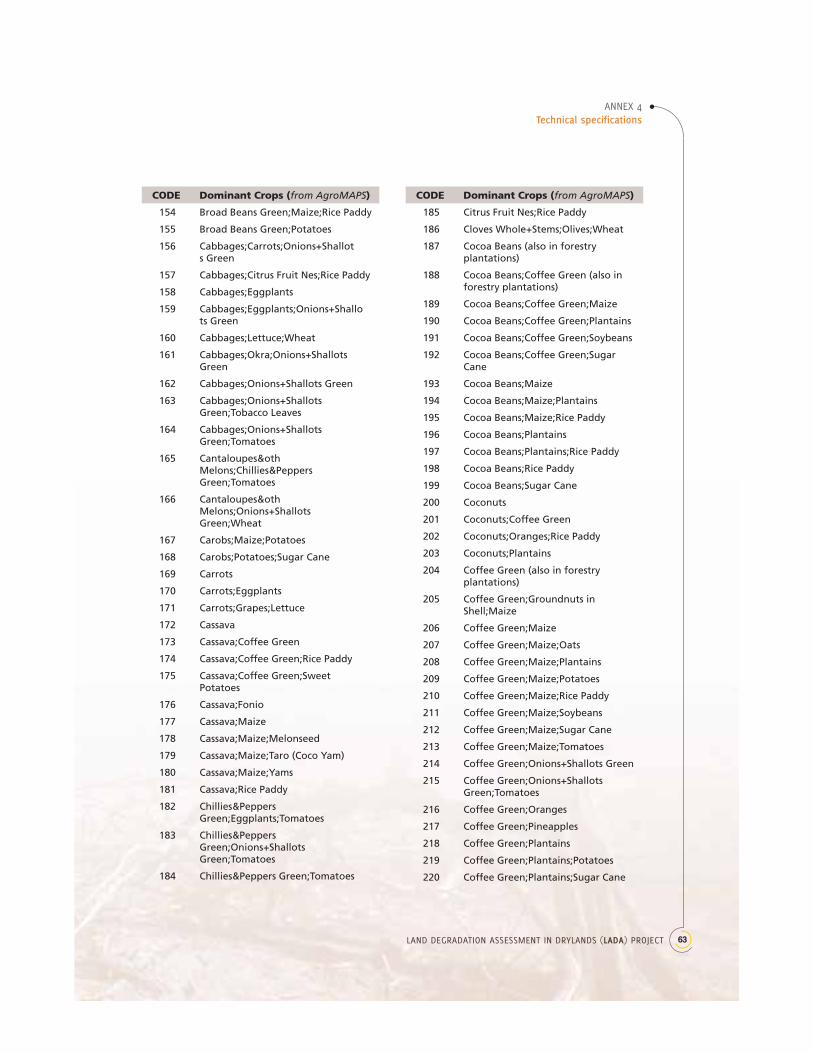
63LAND DEGRADATION ASSESSMENT IN DRYLANDS (LADA) PROJECT
ANNEX 4 Technical specifications
CODE Dominant Crops (from AgroMAPS)
154 Broad Beans Green;Maize;Rice Paddy
155 Broad Beans Green;Potatoes
156 Cabbages;Carrots;Onions+Shallots Green
157 Cabbages;Citrus Fruit Nes;Rice Paddy
158 Cabbages;Eggplants
159 Cabbages;Eggplants;Onions+Shallots Green
160 Cabbages;Lettuce;Wheat
161 Cabbages;Okra;Onions+ShallotsGreen
162 Cabbages;Onions+Shallots Green
163 Cabbages;Onions+ShallotsGreen;Tobacco Leaves
164 Cabbages;Onions+ShallotsGreen;Tomatoes
165 Cantaloupes&othMelons;Chillies&PeppersGreen;Tomatoes
166 Cantaloupes&othMelons;Onions+ShallotsGreen;Wheat
167 Carobs;Maize;Potatoes
168 Carobs;Potatoes;Sugar Cane
169 Carrots
170 Carrots;Eggplants
171 Carrots;Grapes;Lettuce
172 Cassava
173 Cassava;Coffee Green
174 Cassava;Coffee Green;Rice Paddy
175 Cassava;Coffee Green;Sweet Potatoes
176 Cassava;Fonio
177 Cassava;Maize
178 Cassava;Maize;Melonseed
179 Cassava;Maize;Taro (Coco Yam)
180 Cassava;Maize;Yams
181 Cassava;Rice Paddy
182 Chillies&PeppersGreen;Eggplants;Tomatoes
183 Chillies&PeppersGreen;Onions+ShallotsGreen;Tomatoes
184 Chillies&Peppers Green;Tomatoes
CODE Dominant Crops (from AgroMAPS)
185 Citrus Fruit Nes;Rice Paddy
186 Cloves Whole+Stems;Olives;Wheat
187 Cocoa Beans (also in forestry plantations)
188 Cocoa Beans;Coffee Green (also in forestry plantations)
189 Cocoa Beans;Coffee Green;Maize
190 Cocoa Beans;Coffee Green;Plantains
191 Cocoa Beans;Coffee Green;Soybeans
192 Cocoa Beans;Coffee Green;Sugar Cane
193 Cocoa Beans;Maize
194 Cocoa Beans;Maize;Plantains
195 Cocoa Beans;Maize;Rice Paddy
196 Cocoa Beans;Plantains
197 Cocoa Beans;Plantains;Rice Paddy
198 Cocoa Beans;Rice Paddy
199 Cocoa Beans;Sugar Cane
200 Coconuts
201 Coconuts;Coffee Green
202 Coconuts;Oranges;Rice Paddy
203 Coconuts;Plantains
204 Coffee Green (also in forestry plantations)
205 Coffee Green;Groundnuts in Shell;Maize
206 Coffee Green;Maize
207 Coffee Green;Maize;Oats
208 Coffee Green;Maize;Plantains
209 Coffee Green;Maize;Potatoes
210 Coffee Green;Maize;Rice Paddy
211 Coffee Green;Maize;Soybeans
212 Coffee Green;Maize;Sugar Cane
213 Coffee Green;Maize;Tomatoes
214 Coffee Green;Onions+Shallots Green
215 Coffee Green;Onions+Shallots Green;Tomatoes
216 Coffee Green;Oranges
217 Coffee Green;Pineapples
218 Coffee Green;Plantains
219 Coffee Green;Plantains;Potatoes
220 Coffee Green;Plantains;Sugar Cane

MAPPING LAND USE SYSTEMS AT GLOBAL AND REGIONAL SCALES FOR LAND DEGRADATION ASSESSMENT ANALYSISVersion 1.1
64 LAND DEGRADATION ASSESSMENT IN DRYLANDS (LADA) PROJECT
CODE Dominant Crops (from AgroMAPS)
221 Coffee Green;Potatoes
222 Coffee Green;Rice Paddy
223 Coffee Green;Rice Paddy;Vanilla
224 Coffee Green;Sorghum
225 Coffee Green;Soybeans
226 Coffee Green;Sugar Cane
227 Coffee Green;Sugar Cane;Tomatoes
228 Coffee Green;Tea
229 Cow Peas Dry
230 Cow Peas Dry;PepperWhite/Long/Black
231 Cow Peas Dry;Groundnuts in Shell;Maize
232 Cow Peas Dry;Groundnuts in Shell;Millet
233 Cow Peas Dry;Maize
234 Cow Peas Dry;Maize;Sorghum
235 Cow Peas Dry;Millet
236 Cow Peas Dry;Millet;Sorghum
237 Cow Peas Dry;Oil Palm Fruit
238 Cow Peas Dry;Rice Paddy
239 Cow Peas Dry;Sorghum
240 Cow Peas Dry;Soybeans
241 Cucumbers and Gherkins
242 Dates
243 Dates;Citrus Fruit nes;Wheat
244 Dates;Sorghum
245 Dates;Sorghum;Tomatoes
246 Dates;Wheat
247 Dates;Wheat;Sorghum
248 Eggplants;Onions+Shallots Green
249 Eggplants;Onions+ShallotsGreen;Tomatoes
250 Eggplants;Pumpkins Squash Gourds;Tomatoes
251 Eggplants;Tomatoes
252 Fonio;Groundnuts in Shell
253 Fonio;Groundnuts in Shell;Maize
254 Fonio;Groundnuts in Shell;Rice Paddy
255 Fonio;Maize
256 Fonio;Maize;Rice Paddy
CODE Dominant Crops (from AgroMAPS)
257 Fonio;Maize;Sorghum
258 Fonio;Rice Paddy
259 Grapefruit and Pomelos
260 Grapefruit and Pomelos;Oranges
261 Grapes
262 Grapes;Lettuce
263 Grapes;Lettuce;Millet
264 Grapes;Maize
265 Grapes;Maize;Olives
266 Grapes;Maize;Potatoes
267 Grapes;Maize;Soybeans
268 Grapes;Maize;Wheat
269 Grapes;Olives
270 Grapes;Olives;Tomatoes
271 Grapes;Olives;Wheat
272 Grapes;Potatoes
273 Grapes;Potatoes;Wheat
274 Grapes;Sorghum;Wheat
275 Grapes;Wheat
276 Groundnuts in Shell
277 Groundnuts in Shell;Maize
278 Groundnuts in Shell;Maize;Millet
279 Groundnuts in Shell;Maize;Pulses nes
280 Groundnuts in Shell;Maize;Rice Paddy
281 Groundnuts in Shell;Maize;Seed Cotton
282 Groundnuts in Shell;Maize;Sorghum
283 Groundnuts in Shell;Maize;Taro (Coco Yam)
284 Groundnuts in Shell;Maize;Tobacco Leaves
285 Groundnuts in Shell;Maize;Tomatoes
286 Groundnuts in Shell;Millet
287 Groundnuts in Shell;Millet;Rice Paddy
288 Groundnuts in Shell;Millet;Sesame Seed
289 Groundnuts in Shell;Millet;Sorghum
290 Groundnuts in Shell;Millet;Yams
291 Groundnuts in Shell;Oilseeds nes
292 Groundnuts in Shell;Oilseeds nes;Rice Paddy

65LAND DEGRADATION ASSESSMENT IN DRYLANDS (LADA) PROJECT
ANNEX 4 Technical specifications
CODE Dominant Crops (from AgroMAPS)
293 Groundnuts in Shell;Pistachios;Plantains
294 Groundnuts in Shell;Plantains;Taro (Coco Yam)
295 Groundnuts in Shell;Rice Paddy
296 Groundnuts in Shell;Rice Paddy;Sorghum
297 Groundnuts in Shell;Seed Cotton
298 Groundnuts in Shell;Seed Cotton;Soybeans
299 Groundnuts in Shell;Seed Cotton;Sunflower Seed
300 Groundnuts in Shell;Seed Cotton;Wheat
301 Groundnuts in Shell;Sorghum
302 Groundnuts in Shell;Sorghum;Sugar Cane
303 Groundnuts in Shell;Sorghum;Wheat
304 Groundnuts in Shell;Soybeans
305 Groundnuts in Shell;Soybeans;Wheat
306 Groundnuts in Shell;Sunflower Seed
307 Groundnuts in Shell;Sweet Potatoes
308 Groundnuts in Shell;Wheat
309 Lemons and Limes;Maize
310 Lemons and Limes;Maize;Rice Paddy
311 Lemons and Limes;Oranges
312 Lentils;Maize;Potatoes
313 Lentils;Oats
314 Lettuce;Onions+Shallots Green
315 Lupins;Wheat
316 Maize
317 Maize;Groundnuts in Shell
318 Maize;Groundnuts in Shell;Sorghum
319 Maize;Millet
320 Maize;Millet;Rice Paddy
321 Maize;Millet;Sorghum
322 Maize;Millet;Wheat
323 Maize;Oats
324 Maize;Oats;Potatoes
325 Maize;Oats;Soybeans
326 Maize;Oats;Wheat
327 Maize;Oil Palm Fruit
CODE Dominant Crops (from AgroMAPS)
328 Maize;Olives
329 Maize;Onions Dry;Tomatoes
330 Maize;Onions+Shallots Green
331 Maize;Onions+ShallotsGreen;Potatoes
332 Maize;Onions+Shallots Green;Rice Paddy
333 Maize;Onions+Shallots Green;Sugar Cane
334 Maize;Oranges
335 Maize;Oranges;Plantains
336 Maize;Oranges;Wheat
337 Maize;Pigeon Peas
338 Maize;Pistachios
339 Maize;Plantains
340 Maize;Plantains;Potatoes
341 Maize;Plantains;Rice Paddy
342 Maize;Plantains;Soybeans
343 Maize;Plantains;Sugar Cane
344 Maize;Potatoes
345 Maize;Potatoes;Rice Paddy
346 Maize;Potatoes;Soybeans
347 Maize;Potatoes;Sugar Cane
348 Maize;Potatoes;Taro (Coco Yam)
349 Maize;Potatoes;Wheat
350 Maize;Pulses nes
351 Maize;Pulses nes;Sweet Potatoes
352 Maize;Pulses nes;Tobacco Leaves
353 Maize;Rice Paddy
354 Maize;Rice Paddy;Seed Cotton
355 Maize;Rice Paddy;Sorghum
356 Maize;Rice Paddy;Soybeans
357 Maize;Rice Paddy;Sugar Cane
358 Maize;Rice Paddy;Tomatoes
359 Maize;Rice Paddy;Wheat
360 Maize;Rye
361 Maize;Seed Cotton
362 Maize;Seed Cotton;Sorghum
363 Maize;Seed Cotton;Soybeans
364 Maize;Seed Cotton;Sugar Cane
365 Maize;Seed Cotton;Wheat
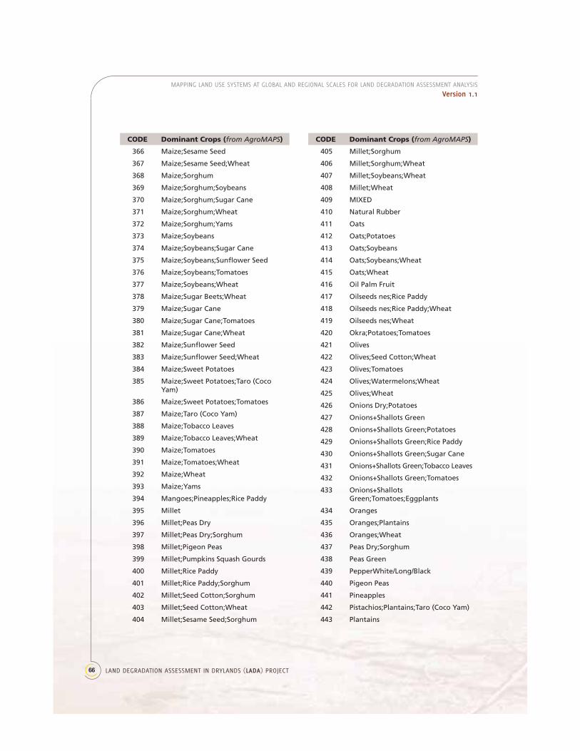
MAPPING LAND USE SYSTEMS AT GLOBAL AND REGIONAL SCALES FOR LAND DEGRADATION ASSESSMENT ANALYSISVersion 1.1
66 LAND DEGRADATION ASSESSMENT IN DRYLANDS (LADA) PROJECT
CODE Dominant Crops (from AgroMAPS)
366 Maize;Sesame Seed
367 Maize;Sesame Seed;Wheat
368 Maize;Sorghum
369 Maize;Sorghum;Soybeans
370 Maize;Sorghum;Sugar Cane
371 Maize;Sorghum;Wheat
372 Maize;Sorghum;Yams
373 Maize;Soybeans
374 Maize;Soybeans;Sugar Cane
375 Maize;Soybeans;Sunflower Seed
376 Maize;Soybeans;Tomatoes
377 Maize;Soybeans;Wheat
378 Maize;Sugar Beets;Wheat
379 Maize;Sugar Cane
380 Maize;Sugar Cane;Tomatoes
381 Maize;Sugar Cane;Wheat
382 Maize;Sunflower Seed
383 Maize;Sunflower Seed;Wheat
384 Maize;Sweet Potatoes
385 Maize;Sweet Potatoes;Taro (Coco Yam)
386 Maize;Sweet Potatoes;Tomatoes
387 Maize;Taro (Coco Yam)
388 Maize;Tobacco Leaves
389 Maize;Tobacco Leaves;Wheat
390 Maize;Tomatoes
391 Maize;Tomatoes;Wheat
392 Maize;Wheat
393 Maize;Yams
394 Mangoes;Pineapples;Rice Paddy
395 Millet
396 Millet;Peas Dry
397 Millet;Peas Dry;Sorghum
398 Millet;Pigeon Peas
399 Millet;Pumpkins Squash Gourds
400 Millet;Rice Paddy
401 Millet;Rice Paddy;Sorghum
402 Millet;Seed Cotton;Sorghum
403 Millet;Seed Cotton;Wheat
404 Millet;Sesame Seed;Sorghum
CODE Dominant Crops (from AgroMAPS)
405 Millet;Sorghum
406 Millet;Sorghum;Wheat
407 Millet;Soybeans;Wheat
408 Millet;Wheat
409 MIXED
410 Natural Rubber
411 Oats
412 Oats;Potatoes
413 Oats;Soybeans
414 Oats;Soybeans;Wheat
415 Oats;Wheat
416 Oil Palm Fruit
417 Oilseeds nes;Rice Paddy
418 Oilseeds nes;Rice Paddy;Wheat
419 Oilseeds nes;Wheat
420 Okra;Potatoes;Tomatoes
421 Olives
422 Olives;Seed Cotton;Wheat
423 Olives;Tomatoes
424 Olives;Watermelons;Wheat
425 Olives;Wheat
426 Onions Dry;Potatoes
427 Onions+Shallots Green
428 Onions+Shallots Green;Potatoes
429 Onions+Shallots Green;Rice Paddy
430 Onions+Shallots Green;Sugar Cane
431 Onions+Shallots Green;Tobacco Leaves
432 Onions+Shallots Green;Tomatoes
433 Onions+ShallotsGreen;Tomatoes;Eggplants
434 Oranges
435 Oranges;Plantains
436 Oranges;Wheat
437 Peas Dry;Sorghum
438 Peas Green
439 PepperWhite/Long/Black
440 Pigeon Peas
441 Pineapples
442 Pistachios;Plantains;Taro (Coco Yam)
443 Plantains
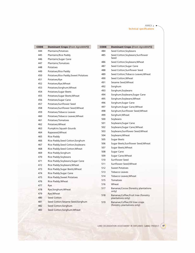
67LAND DEGRADATION ASSESSMENT IN DRYLANDS (LADA) PROJECT
ANNEX 4 Technical specifications
CODE Dominant Crops (from AgroMAPS)
444 Plantains;Potatoes
445 Plantains;Rice Paddy
446 Plantains;Sugar Cane
447 Plantains;Tomatoes
448 Potatoes
449 Potatoes;Rice Paddy
450 Potatoes;Rice Paddy;Sweet Potatoes
451 Potatoes;Rye
452 Potatoes;Rye;Wheat
453 Potatoes;Sorghum;Wheat
454 Potatoes;Sugar Beets
455 Potatoes;Sugar Beets;Wheat
456 Potatoes;Sugar Cane
457 Potatoes;Sunflower Seed
458 Potatoes;Sunflower Seed;Wheat
459 Potatoes;Tobacco Leaves
460 Potatoes;Tobacco Leaves;Wheat
461 Potatoes;Tomatoes
462 Potatoes;Wheat
463 Pumpkins Squash Gourds
464 Rapeseed;Wheat
465 Rice Paddy
466 Rice Paddy;Seed Cotton;Sorghum
467 Rice Paddy;Seed Cotton;Soybeans
468 Rice Paddy;Seed Cotton;Wheat
469 Rice Paddy;Sorghum
470 Rice Paddy;Soybeans
471 Rice Paddy;Soybeans;Sugar Cane
472 Rice Paddy;Soybeans;Wheat
473 Rice Paddy;Sugar Beets;Wheat
474 Rice Paddy;Sugar Cane
475 Rice Paddy;Sweet Potatoes
476 Rice Paddy;Wheat
477 Rye
478 Rye;Sorghum;Wheat
479 Rye;Wheat
480 Seed Cotton
481 Seed Cotton;Sesame Seed;Sorghum
482 Seed Cotton;Sorghum
483 Seed Cotton;Sorghum;Wheat
CODE Dominant Crops (from AgroMAPS)
484 Seed Cotton;Soybeans
485 Seed Cotton;Soybeans;Sunflower Seed
486 Seed Cotton;Soybeans;Wheat
487 Seed Cotton;Sugar Cane
488 Seed Cotton;Sunflower Seed
489 Seed Cotton;Tobacco Leaves;Wheat
490 Seed Cotton;Wheat
491 Sesame Seed;Wheat
492 Sorghum
493 Sorghum;Soybeans
494 Sorghum;Soybeans;Sugar Cane
495 Sorghum;Soybeans;Wheat
496 Sorghum;Sugar Cane
497 Sorghum;Sugar Cane;Wheat
498 Sorghum;Sunflower Seed;Wheat
499 Sorghum;Wheat
500 Soybeans
501 Soybeans;Sugar Cane
502 Soybeans;Sugar Cane;Wheat
503 Soybeans;Sunflower Seed;Wheat
504 Soybeans;Wheat
505 Sugar Beets
506 Sugar Beets;Sunflower Seed;Wheat
507 Sugar Beets;Wheat
508 Sugar Cane
509 Sugar Cane;Wheat
510 Sunflower Seed
511 Sunflower Seed;Wheat
512 Sweet Potatoes
513 Tobacco Leaves
514 Tobacco Leaves;Wheat
515 Tomatoes
516 Wheat
517 Bananas;Cocoa (forestry plantations only)
518 Bananas;Coffee;Fruit tree (forestry plantations only)
519 Bananas;Coffee;Oil tree crops (forestry plantations only)

MAPPING LAND USE SYSTEMS AT GLOBAL AND REGIONAL SCALES FOR LAND DEGRADATION ASSESSMENT ANALYSISVersion 1.1
68 LAND DEGRADATION ASSESSMENT IN DRYLANDS (LADA) PROJECT
CODE Dominant Crops (from AgroMAPS)
520 Bananas;Coffee;Spices (forestry plantations only)
521 Bananas;Fruit tree (forestry plantations only)
522 Bananas;Fruit tree;Oil tree crops (forestry plantations only)
523 Bananas;Oil tree crops (forestry plantations only)
524 Bananas;Rubber & other crops (forestry plantations only)
525 Bananas;Spices (forestry plantations only)
526 Coffee;Fruit tree (forestry plantations only)
527 Coffee;Oil tree crops (forestry plantations only)
528 Coffee;Rubber & other crops (forestry plantations only)
529 Coffee;Spices (forestry plantations only)
530 Fruit tree (forestry plantations only)
531 Fruit tree;Oil tree crops (forestry plantations only)
532 Oil tree crops (forestry plantations only)
533 Rubber & other crops (forestry plantations only)
534 Spices (forestry plantations only)
Land Use Attributes – Dominant crops (from IFPRI)In the case of IFPRI data, the dominant crop is a single one and is listed in 20 classes in alphabetical order. This attribute is present only where Agro-MAPS has NO DATA.
CODE Dominant Crops (from IFPRI)
-999 None
1 Bananas & plantains
2 Barley
3 Beans
4 Cassava
5 Coffee
6 Cotton
7 Groundnut
8 Maize
9 Millet
10 Other fibers crop
11 Other oils crop
12 Other pulse crops
13 Potatoes
14 Rice
15 Sorghum
16 Soybean
17 Sugar beat
18 Sugar cane
19 Sweet potatoes & yams
20 Wheat
Land Use Attributes – Dominant crop groups (from AgroMAPS)The dominant crops are listed in 90 classes in alphabetical order. This attribute shows crop groups in cropland areas only.
CODE Crop groups
-999 Not available
1 Cereals and cereal products
2 Cereals and cereal products;Fruits
3 Cereals and cereal products;Fruits;Oil-bearing crops
4 Cereals and cereal products;Fruits;Pulses
5 Cereals and cereal products;Fruits;Roots tubers

69LAND DEGRADATION ASSESSMENT IN DRYLANDS (LADA) PROJECT
ANNEX 4 Technical specifications
CODE Crop groups
6 Cereals and cereal products;Fruits;Stimulant crops
7 Cereals and cereal products;Fruits;Sugar crops and sweeteners
8 Cereals and cereal products;Fruits;Vegetables
9 Cereals and cereal products;Nuts
10 Cereals and cereal products;Oil-bearing crops
11 Cereals and cereal products;Oil-bearing crops;Fruits
12 Cereals and cereal products;Oil-bearing crops;Pulses
13 Cereals and cereal products;Oil-bearing crops;Roots tubers
14 Cereals and cereal products;Oil-bearing crops;Stimulant crops
15 Cereals and cereal products;Oil-bearing crops;Sugar crops and sweeteners
16 Cereals and cereal products;Oil-bearing crops;Vegetables
17 Cereals and cereal products;Pulses
18 Cereals and cereal products;Pulses;Roots tubers
19 Cereals and cereal products;Pulses;Stimulant crops
20 Cereals and cereal products;Pulses;Sugar crops and sweeteners
21 Cereals and cereal products;Pulses;Vegetables
22 Cereals and cereal products;Roots tubers
23 Cereals and cereal products;Roots tubers;Stimulant crops
24 Cereals and cereal products;Roots tubers;Sugar crops and sweeteners
25 Cereals and cereal products;Roots tubers;Tobacco rubber and other crops
26 Cereals and cereal products;Roots tubers;Vegetables
27 Cereals and cereal products;Stimulant crops
CODE Crop groups
28 Cereals and cereal products;Stimulant crops;Sugar crops and sweeteners
29 Cereals and cereal products;Stimulant crops;Vegetables
30 Cereals and cereal products;Sugar crops and sweeteners
31 Cereals and cereal products;Sugar crops and sweeteners;Vegetables
32 Cereals and cereal products;Tobacco rubber and other crops
33 Cereals and cereal products;Vegetables
34 Fruits
35 Fruits;cereals and cereal products
36 Fruits;Nuts;Roots tubers
37 Fruits;Oil-bearing crops
38 Fruits;Oil-bearing crops;Roots tubers
39 Fruits;Pulses
40 Fruits;Pulses;Roots tubers
41 Fruits;Pulses;Stimulant crops
42 Fruits;Pulses;Sugar crops and sweeteners
43 Fruits;Roots tubers
44 Fruits;Roots tubers;Stimulant crops
45 Fruits;Roots tubers;Sugar crops and sweeteners
46 Fruits;Roots tubers;Vegetables
47 Fruits;Stimulant crops
48 Fruits;Stimulant crops;Sugar crops and sweeteners
49 Fruits;Sugar crops and sweeteners
50 Fruits;Vegetables
51 Mixed
52 Nuts;Oil-bearing crops
53 Oil-bearing crops
54 Oil-bearing crops;cereals and cereal products
55 Oil-bearing crops;Fruits
56 Oil-bearing crops;Fruits;cereals and cereal products
57 Oil-bearing crops;Pulses
58 Oil-bearing crops;Pulses
59 Oil-bearing crops;Roots tubers

MAPPING LAND USE SYSTEMS AT GLOBAL AND REGIONAL SCALES FOR LAND DEGRADATION ASSESSMENT ANALYSISVersion 1.1
70 LAND DEGRADATION ASSESSMENT IN DRYLANDS (LADA) PROJECT
CODE Crop groups
60 Oil-bearing crops;Stimulant crops
61 Oil-bearing crops;Sugar crops and sweeteners
62 Oil-bearing crops;Vegetables
63 Pulses
64 Pulses;Roots tubers
65 Pulses;Roots tubers;Stimulant crops
66 Pulses;Roots tubers;Sugar crops and sweeteners
67 Pulses;Roots tubers;Vegetables
68 Pulses;spices
69 Pulses;Stimulant crops
70 Pulses;Stimulant crops;Sugar crops and sweeteners
71 Pulses;Sugar crops and sweeteners
72 Pulses;Vegetables
73 Roots tubers
74 Roots tubers;Fruits;cereals and cereal products
75 Roots tubers;Stimulant crops
76 Roots tubers;Stimulant crops;Sugar crops and sweeteners
77 Roots tubers;Sugar crops and sweeteners
78 Roots tubers;Sugar crops and sweeteners;Tobacco rubber and other crops
79 Roots tubers;Tobacco rubber and other crops
80 Roots tubers;Vegetables
81 Spices
82 Stimulant crops
83 Stimulant crops;Sugar crops and sweeteners
84 Stimulant crops;Sugar crops and sweeteners;Vegetables
85 Stimulant crops;Vegetables
86 Sugar crops and sweeteners
87 Sugar crops and sweeteners;Vegetables
88 Tobacco rubber and other crops
89 Vegetables
90 Vegetables;cereals and cereal products
Land Use Attributes – Dominant crop groups (from AgroMAPS)Irrigation has been reclassified in only 2 classes, low (i.e. small-scale) or large-scale irrigation. Low-scale irrigation may be present in all LUS classes while large-scale irrigation is a subclass associated with the agricultural or agro-pastoral classes.
CODE Irrigation
-999 None
1 Low-scale irrigation
2 Large-scale irrigation
Land Use Attributes – Agricultural management indexThe management index has been reclassified in 6 classes and is present, when available, in agricultural areas and in forested areas with agricultural activities.
CODE Management
0 Not available
1 Very poor managed
2 Relatively poor managed
3 Well managed
4 Very well managed
5 Relatively over managed
6 Over managed
7 No data
Biophysical Attributes – Length of Growing Period (LGP) classesThe LGP is subdivided in 14 classes from the driest to the more humid class, with the unit of measurement being number of 30 days (month) periods.

71LAND DEGRADATION ASSESSMENT IN DRYLANDS (LADA) PROJECT
ANNEX 4 Technical specifications
CODE LGP
1 0
2 1 to 29
3 30 to 59
4 60 to 89
5 90 to 119
6 120 to 149
7 150 to 179
8 180 to 209
9 210 to 239
10 240 to 269
11 270 to 299
12 300 to 329
13 330 to 359
14 above 360
Biophysical Attributes of the Ecosystem: dominant soilsThe soils are extrapolated from the Harmonized World Soil Database and are subdivided in 35classes. In the case of ESRI GRID version the soil symbol is not used. The “not defined” class may depend from differences between coastlines of different LUS dataset (note that water has also been inserted in this class). The “no data” class is derived from the original HWSD.
CODE SOIL SYMBOL
-999 Not Defined NI
1 Acrisols AC
2 Alisols AL
3 Andosols AN
4 Arenosols AR
5 Anthrosols AT
6 Chernozems CH
7 Calcisols CL
8 Cambisols CM
9 Fluvisols FL
10 Ferralsols FR
CODE SOIL SYMBOL
11 Gleysols GL
12 Greyzems GR
13 Gypsisols GY
14 Histosols HS
15 Kastanozems KS
16 Leptosols LP
17 Luvisols LV
18 Lixisols LX
19 Nitisols NT
20 Podzoluvisols PD
21 Phaeozems PH
22 Planosols PL
23 Plinthosols PT
24 Podzols PZ
25 Regosols RG
26 Solonchaks SC
27 Solonetz SN
28 Vertisols VR
29 Rock Outcrop RK
30 Sand Dunes DS
32 Urban, mining UR
31
33 Salt Flats ST
34 No data NI
35 Glaciers GG
36 Island IS
Biophysical Attributes – Slope classesThe slope percentage was derived from SRTM and is subdivided in 10 classes, where 0 indicates areas that are “undefined” in the source data. In other cases, the Land Use System map may have a different coastline than the slope map (derived from SRTM Shuttle mission). In those cases the code -999 is used and the label is “not available”.

MAPPING LAND USE SYSTEMS AT GLOBAL AND REGIONAL SCALES FOR LAND DEGRADATION ASSESSMENT ANALYSISVersion 1.1
72 LAND DEGRADATION ASSESSMENT IN DRYLANDS (LADA) PROJECT
CODE Slope
-999 Not available
0 Undefined
1 0 to 0.5
2 0.5 to 2
3 2 to 5
4 5 to 8
5 8 to 16
6 16 to 30
7 30 to 45
8 above 45
Socio-Economic Attributes – Population densityThe population density, measured in inhabitants per square kilometres, is classified into 7 classes, where -999 defines areas with no data.
CODE Population density
-999 Undefined
1 0
2 0 to 2
3 2 to 10
4 10 to 50
5 50 to 250
6 above 250
Socio-Economic Attributes – Infant mortality rateThe infant mortality rate (the number of children out of every 1000 born alive that die before they reach the age of one year) is classified in 11 classes, where -999 defines areas with no data.
CODE Poverty
-999 Undefined
1 below 2
2 2 to 5
3 5 to 10
4 10 to 20
5 20 to 30
6 30 to 40
7 40 to 50
8 50 to 75
9 75 to 100
10 above 100
Quality of the databaseData quality was and remains a major concern. Putting together global data layers of variable quality and different resolutions / scales by simple overlay is a risky exercise, which is bound to result in some erroneous conclusions being drawn on the land use systems practiced. Major problems with the individual databases used are well known (FAO, 2005) and are discussed in this Manual (section 1.3).
This section aims to describe some of the methods used to reduce this problem.
Position accuracyMost databases used came from FAO internal sources, which had already been corrected for positional accuracy.
In other cases, some correction needs to be done. For example, the FAO/IIASA GAEZ data (i.e. LGP, thermal climate and slope (the SRTM corrected data was resampled by IIASA)), the boundaries were buffered in order that a simple clipping was realistic. The soil map (from the beta version of the Harmonized World Soil Database) was corrected to match with GAUL by IIASA.
73LAND DEGRADATION ASSESSMENT IN DRYLANDS (LADA) PROJECT
ANNEX 4 Technical specifications
Expansion of outer boundaries and clipping was performed using a reference layer at a 5 arc minutes resolution. Data were in all cases first re-classified, secondly resampled and finally compared to the reference layer. Subsequently, the re-sampling technique was applied with a snap to the reference grid.
The datasets where major problems were encountered were the population density and livestock maps.
Completeness The work previously described allowed to create a quite consistent database in term of completeness. Less than 150 pixels (of over more than 2 million) in islands or far northern areas have most of the attribute missing.
The incompleteness of the Agro-Maps database has been highlighted within this Manual (section 4.2), but missing data have been consistently substituted (as a separate attribute) by IFPRI data. Nevertheless there are a few areas were neither of the datasets held information.
CorrectnessThe correctness of this database is linked to the correctness of each single input layer.
Timeliness Integrating this amount of different data creates issues of time precision which must be borne in mind when using the outputs. Data sources were from the nineties (Agro-MAPS) to 2007 in the case of Global Map of Irrigated areas. In case of IFPRI beta version, the year of data collection is unknown.

References
Bai, Z.G. & Dent D.L. 2007. Assessment of Land Degradation and Improvement in South Africa. LADA Project, internal document.
Bai, Z.G., Dent, D.L., Olson. L. & Schaepman, M. 2008. Global land degradation assessment. (in preparation).
CDE/WOCAT, FAO/LADA, ISRIC. 2011. Questionnaire for Mapping Land Degradation and Sustainable Land Management v2. WOCAT, Berne, Switzerland.
Centre for International Earth Science Information Network (CIESIN), Columbia University. 2005. Global subnational infant mortality rates.CIESIN, Palisades, NY, USA. Available from: http://www.ciesin.columbia.edu/povmap/ds_global.html [Accessed 18 November 2007].
Centre de Suivi Ecologique (CSE). 2007a. Préparation du guide pour la stratification, Rapport intérimaire 1. LADA Project Senegal country report. Available from: http://www.fao.org/nr/lada/index.php?option=com_docman&task=cat_view&gid=53&Itemid=165&lang=en.
Centre de Suivi Ecologique (CSE). 2007b. Préparation du guide pour la stratification, Rapport intérimaire 2. LADA Project Senegal country report.
Centre de Suivi Ecologique (CSE). 2008. Préparation du guide pour la stratification, Rapport intérimaire 3. LADA Project Senegal country report.
China LADA team. 2008. Land use system map of China. LADA project China country report. Available from: http://www.fao.org/nr/lada/index.php?option=com_docman&task=doc_download&gid=763&Itemid=165&lang=en.
Direction Générale de l’Aménagement et la Conservation des Terres Agricoles.2008. Réalisation d’une carte d’utilisation des terres à l’échelle 1/500 000 en se basant sur des données nationales disponibles et en suivant les directives LADA pour la starification et la cartographie LUS. LADA Project Tunisia country report.
Dixon, J, Gulliver, Gibbon, D. 2001. Farming Systems and Poverty - Improving farmers’ livelihoods in a changing world. FAO and World Bank, Rome and Washington DC. 412p.

MAPPING LAND USE SYSTEMS AT GLOBAL AND REGIONAL SCALES FOR LAND DEGRADATION ASSESSMENT ANALYSISVersion 1.1
76 LAND DEGRADATION ASSESSMENT IN DRYLANDS (LADA) PROJECT
European Space Agency (ESA) GlobCover Project. 2008. GlobCover Land Cover v2 2008 database, led by MEDIAS-France. Available from: http://ionia1.esrin.esa.int/index.asp [Accessed 22 July 2011].
FAO. 1978-1981. Report on the agro-ecological zones project. Vol 1 Methodology and Results for Africa. Vol. 2 - Results for Southwest Asia. Vol 3. South America. Vol 4 Southeast Asia. World Soil Resources Reports No 48. Food and Agriculture Organization of the United Nations, Rome, Italy.
FAO. 1992. Agro-Ecological Zoning Guidelines. FAO Soils Bulletin 73. Food and Agriculture Organization of the United Nations, Rome, Italy.
FAO. 2005. An inventory and comparison of globally consistent geospatial databases and libraries. Environmental and Natural Resources Working Paper 19. Food and Agriculture Organization of the United Nations, Rome, Italy.
FAO. 2005. Reports of the series of Global Land Cover Network Training Workshops,Food and Agriculture Organization of the United Nations, Rome, Italy.
FAO/IFPRI/SAGE. 2006. Agro-MAPS. FAO Land and Water Digital media series # 32. Food and Agriculture Organization of the United Nations, Rome, Italy.
FAO. 2007. Consultant Report on Global LADA Stratification Data for China.LADA Project, internal document. Food and Agriculture Organization of the United Nations, Rome, Italy.
FAO/IIASA/ISRIC/JRC & C-AS. 2008. Harmonized World Soil Database. FAO Land and Water Digital Media Series # 34. Food and Agriculture Organization of the United Nations, Rome, Italy. Latest revision available at: http://www.fao.org/nr/land/soils/harmonized-world-soil-database/en/ [Accessed 23 July 2011].
FAO/IIASA, 2010. Global Agro-ecological Zoning. FAO Land and Water Digital Media series # 35. Food and Agriculture Organization of the United Nations, Rome, Italy. Available from: http://www.gaez.iiasa.ac.at/w/ctrl?_flow=Vwr&_view=Welcome&idAS=0&idFS=0&fieldmain=main_&idPS=0 [Accessed 22 July 2011].
FAO-WOCAT. 2011. Questionnaire for Mapping Land Degradation and Sustainable Land Management (QM) v2. Food and Agriculture Organization of the United Nations, Rome, Italy.
Fischer, G., van Velthuizen, Shah, M. & Nachtergaele, F. 2002. Global agro-ecological assessment for agriculture in the 21st century. IIASA/FAO. 119p.
Fischer, G. 2009. Personal communication.George, H. & Petri, M. 2006. The rapid characterization and mapping of
agricultural land-use: A methodological framework approach for the LADA project. LADA Project technical report 1. Available from: http://www.fao.org/nr/lada/index.php?option=com_docman&task=doc_download&gid=11&Itemid=165&lang=en [Accessed 22 July 2011].
JRC. 2005. GLC 2000, a New Approach to Global Land Cover Mapping from Earth Observation Data. Intern. Journal of Remote Sensing Volume 26, Number 9, pp.1959-1977(19). Available from: http://www.ingentaconnect.com/content/tandf/tres/2005/00000026/00000009/art00012 [Accessed 22 July 2011].
FAO-WOCAT. 2011. Questionnaire for Mapping Land Degradation and Sustainable

77LAND DEGRADATION ASSESSMENT IN DRYLANDS (LADA) PROJECT
References
IIASA. 2009. Compilation of selected global indicator of land degradation. LADA technical report 14. Available from: http://www.fao.org/nr/lada/index.php?option=com_docman&task=doc_download&gid=331&Itemid=165&lang=en.
Monfreda, C., Ramankutty, N. & Foley, J.A. 2008. Farming the Planet. 2: The Geographic Distribution of Crop Areas and Yields in the Year 2000, Glob. Biogeochem. Cycles, submitted.
Ravelo, A. et al. 2010. Unpublished LADA land use system report of Argentina.Ravelo, A.C., Planchuelo, A.M., Kindgard, A. & Castellanos, M. 2010.
Protocolo de validacion de LUS (proyecto LADA / FAO). LADA Project Argentina country report.
Siebert, S., Döll, P., Feick, S., Hoogeveen, J. & Frenken, K. 2007. Global Map of Irrigation Areas version 4.0.1. Johann Wolfgang Goethe University, Frankfurt am Main, Germany / Food and Agriculture Organization of the United Nations, Rome, Italy. Available from: http://www.fao.org/nr/water/aquastat/irrigationmap/index.stm [Accessed 22 July 2011]
Thornton, P.K., Kruska, R.L., Henninger, N., Kristjanson, P.M., Reid, R.S., Atieno, F., Odero, A.N. & Ndegwa, T. 2002. Mapping poverty and livestock in the developing world. ILRI (International Livestock Research Institute),Nairobi, Kenya.124 pp. Available from: http://www.ilri.org/InfoServ/Webpub/fulldocs/mappingPLDW/index.htm
Tiffen, M. & Mortimore, M. 1992. Environment, Population Growth and Productivity in Kenya: A Case Study of Machakos District. Development Policy Review, Vol. 10, No 1: 359-387.
Wint, G.R.W. & Robinson, T.P. 2007. Gridded Livestock of the World, 2007.Rome: Food and Agriculture. Organization of the United Nations, Animal Production and Health Division. Available from: http://www.fao.org/ag/againfo/resources/en/glw/default.html [Accessed 22 July 2011]
World Conservation Union and UNEP-World Conservation Monitoring Centre. 2007. World Database on Protected Areas, WCMC, Cambridge, UK, 2007.
You, L. & Wood, S. 2006. An entropy approach to spatial disaggregation of agricultural production. Agricultural Systems 90(1-3): 329-347. Available from: http://rustmapper.ctl1.com/YouWood_AgSystem2006.pdf [Accessed 22 July 2011]
Young, A., Bot, A. & Nachtergaele, F. 2000. Land resource potential and constraints at regional and country levels. World Soil Resources Reports no 90. FAO, Rome.

ISRIC
LADA Secretariat Food and Agriculture Organization of the United Nations
Viale delle Terme di Caracalla00153 Rome, ItalyTel.: +39 06570 54888 Fax: +39 06570 [email protected]://www.fao.org/nr/lada I3242/1/03.13
ISBN 978-92-5-107568-5
9 7 8 9 2 5 1 0 7 5 6 8 5