
Manufacturing (co)agglomeration in a transition country ...
64
DOCUMENT DE TRAVAIL / WORKING PAPER No. 2018-16 Manufacturing (co)agglomeration in a transition country: Evidence from Russia Ekaterina Aleksandrova, Kristian Behrens et Maria Kuznetsova Mars 2018
Transcript of Manufacturing (co)agglomeration in a transition country ...

DOCUMENT DE TRAVAIL / WORKING PAPER
No. 2018-16
Manufacturing (co)agglomeration in a transition country: Evidence from
Russia
Ekaterina Aleksandrova, Kristian Behrens et Maria Kuznetsova
Mars 2018

Manufacturing (co)agglomeration in a transition country: Evidence from Russia
Ekaterina Aleksandrova, National Research University Higher School of Economics, Russie
Kristian Behrens, Université du Québec à Montréal, Canada; National Research University Higher School of Economics, Russie; et CEPR
Maria Kuznetsova, National Research University Higher School of Economics, Russie
Document de travail No. 2018-16
Mars 2018
Département des Sciences Économiques Université du Québec à Montréal
Case postale 8888, Succ. Centre-Ville
Montréal, (Québec), H3C 3P8, Canada Courriel : [email protected]
Site web : http://economie.esg.uqam.ca
Les documents de travail contiennent souvent des travaux préliminaires ou partiels et sont circulés pour encourager et stimuler les discussions. Toute citation et référence à ces documents devrait tenir compte de leur caractère provisoire. Les opinions exprimées dans les documents de travail sont ceux de leurs auteurs et ne reflètent pas nécessairement ceux du département des sciences économiques ou de l'ESG.
Copyright (2018): Ekaterina Aleksandrova, Kristian Behrens et Maria Kuznetsova. De courts extraits de texte peuvent être cités et reproduits sans permission explicite à condition que la source soit référencée de manière appropriée.

Manufacturing (co)agglomeration in a transition
country: Evidence from Russia*
Ekaterina Aleksandrova† Kristian Behrens‡
Maria Kuznetsova§
March 9, 2018
Abstract
We document geographic concentration patterns of Russian manufacturing
using microgeographic data. About 42–52% of 4-digit and 63–75% of 3-digit in-
dustries are localized, with a higher share in the European part than in the Asian
part. About 70% of 3-digit industry pairs are coagglomerated, especially those
with stronger buyer-supplier links, more knowledge sharing, and lower transport
costs. Pairs with a more similar workforce are, however, less coagglomerated,
which points to impediments in labor mobility between regions and firms. Over-
all, the agglomeration forces are fairly similar to those operating in developed
countries, with transportation likely to be a key driver.
Keywords: agglomeration; coagglomeration; determinants of geographic con-
centration; manufacturing industries; Russia.
JEL classification: R12
*Behrens gratefully acknowledges financial support from the crc Program of the Social Sciences and Hu-
manities Research Council (sshrc) of Canada for the funding of the Canada Research Chair in Regional Impacts of
Globalization. This study was funded by the Russian Academic Excellence Project ‘5-100’. The views expressed in
this paper and any remaining errors are ours.†National Research University Higher School of Economics, Russia. E-mail: [email protected]‡Corresponding author: Department of Economics, Université du Québec à Montréal, Canada; National Research
University Higher School of Economics, Russia; and cepr, UK. E-mail: [email protected]§National Research University Higher School of Economics, Russia. E-mail: [email protected]
1

1 Introduction
The uneven spatial distribution of industries is a first-order feature of almost any country in
the world. While this has been extensively documented for developed countries—especially for
manufacturing—there is a dearth of evidence for developing or transition countries (see World
Bank, 2009; Duranton, 2015). This is unfortunate because it is precisely for those countries that
understanding geographic concentration—especially for manufacturing—and the associated
productivity gains is important to assess economic development prospects and options.
There is now a broad consensus that agglomeration has a causal effect on productivity due
to the existence of agglomeration economies: doubling the size of an industry in a geographic
area increases productivity by about 2–5% on average (Rosenthal and Strange, 2004; Melo,
Graham, and Noland, 2009; Combes and Gobillon, 2015). Realizing these productivity gains
from geographic concentration may be especially important for transition countries such as
Russia. It has repeatedly been pointed out that Russia needs to reduce its dependence on oil
and primary goods, and that it must substantially improve its weak manufacturing produc-
tivity. According to Deloitte’s 2016 Global Manufacturing Competitiveness Index, Russia ranks 32
out of 40 countries—lower than Brazil, South Africa, and Poland. It has lost 4 ranks since 2013
and is projected to stay at its current rank in 2020.1 There is clearly room for substantial im-
provements, and those may be partly achieved by policies that require a better understanding
of geographic concentration patterns and their underlying determinants.
The aim of our paper is twofold. First, we provide a detailed picture of the geographic
concentration patterns of Russian manufacturing industries. Using recent and highly disaggre-
gated point-pattern data, we estimate the agglomeration of industries and the coagglomeration
of industry pairs.2 We pay specific attention to Russia’s ‘dual geographic structure’, i.e., the
existence of a dense western and a scattered eastern part. Second, we investigate the determi-
1Available online at https://www2.deloitte.com/global/en/pages/manufacturing/articles/global-
manufacturing-competitiveness-index.html, last accessed on February 15, 2018. According to the Global Com-
petitiveness Report 2014–2015, Russia ranks 119 out of 144 countries in terms of its goods market competition and
efficiency. See http://www3.weforum.org/docs/WEF_GlobalCompetitivenessReport_2014-15.pdf, last accessed
on February 20, 2018.2There are only few works on geographic concentration in Russia. They all use either the Herfindal-Hirschman
Index, or the Krugman Dissimilarity Index, or the Theil Index; and all rely on fairly aggregated regional and
industrial data. See, e.g., Kolomak (2015); Rastvortseva and Chentsova (2015); and Maslikhina (2017). We are
aware of two papers that use more disaggregated data. Vorobyev, Kislyak, and Davidson (2010) use a sample of
about 10,000 firms coded to the city level to estimate localization and urbanization economies for different broad
industries. Kofanov, Mihailova, and Shurygin (2015) use a sample of plants—taken from the industrial census
of the USSR in 1989 and coded to the settlement level—to look for differences in the geographic structure of
manufacturing industries between the Soviet state-planned economy and the free market economy starting in the
early 1990s. Neither paper provides estimates for coagglomeration patterns of industry pairs or an analysis of the
determinants of agglomeration.
2
nants of the geographic concentration of individual industries and of the coagglomeration of
industry pairs. Little is known to our knowledge about the former, whereas the latter has not
been investigated at all for Russia until now. Using high-quality Canadian and U.S. industry-
level data to proxy missing Russian data, we investigate how buyer-supplier links, similarity
in labor requirements, knowledge sharing, and transportation costs drive the agglomeration
and coagglomeration of industries. Understanding the role played by these economic vari-
ables is key in devising policies that aim to harness the potential productivity gains from the
geographic concentration of industries.
Our key results may be summarized as follows. First, we document strong spatial patterns.
About 42–52% of 4-digit industries and 63–75% of 3-digit industries are significantly agglom-
erated, with a substantially higher share in the European part than in the Asian part of Russia.
Roughly 70% of industry pairs are significantly coagglomerated, mainly at short distances
below 100 kilometers. Second, the overall patterns of geographic concentration—both their
extent, strength, and composition—are surprisingly similar to those documented for manufac-
turing industries in other countries such as the UK, Canada, or the U.S. Hence, geographic
concentration seems to obey similar rules, despite Russia’s long history of a centrally-planned
economy that explains in large part the geographic structure of industry before 1990 (e.g.,
Kofanov et al., 2015). Third, we find that the mechanisms associated with geographic concen-
tration in Russia are also similar to those operating in other countries. Stronger buyer-supplier
links yield more geographically concentrated patterns, and the same holds true for industry
pairs that exchange more knowledge as measured by patent citations data. The only substan-
tive difference that we find compared to other countries is that industries with a more similar
workforce tend to be less coagglomerated. This may be explained by specific aspects of the
Russian labor market, where low-skilled workers in manufacturing—the bulk of the work-
force in that sector—are not mobile between regions and firms. Furthermore, firm-specific
non-portable training of the workforce further reduces the mobility of workers between firms.
One of our most interesting findings is the key role played by transport costs. We consis-
tently find that industries that face higher transport costs—measured using industry-level ad
valorem trucking costs—are more geographically dispersed than industries that face lower
transport costs. This finding, which is in line with the new economic geography (Krug-
man, 1991) and with recent evidence for Canada (see Behrens, Bougna, and Brown, 2018;
and Behrens and Brown, 2018), suggests that geographic concentration is stronger when trans-
port costs are low. It hints at one policy lever that may be used to potentially influence the
spatial structure of economic activity and to obtain more agglomeration. This finding may be
important for Russia. Although there is substantial infrastructure in the western part of the
country, the transport system is partially overloaded, is being worn out rapidly through exces-
sive use, and degrades quickly do to its inferior quality.3 In the rest of the country, especially
3According to the Global Competitiveness Report 2014–2015, Russia ranks 124 out of 144 countries in terms of
3

the east and the far east, infrastructure is either non-existent or close to being non-existent.
Our results suggest that cheap transportation—via better infrastructure and more deregulated
transport markets—may be required to increase geographic concentration. Yet, one needs to
keep in mind that this may give rise to persistent patterns of regional divergence, where most
economic activity is concentrated in a few core regions at the expense of relatively deserted
peripheries. Such a development would conflict with most regional development objectives for
Russian regions that rank traditionally high on the policy agenda.4
The remainder of the paper is structured as follows. Section 2 briefly presents our data.
Section 3 explains our estimation strategy and summarizes our results for the agglomeration
of individual manufacturing industries and the coagglomeration of industry pairs. We provide
results for all of Russia, as well as for the western and the eastern parts separately. Section 4
contains our analysis of the determinants of agglomeration and coagglomeration in Russia. Fi-
nally, Section 5 concludes and discusses the policy implications of our main findings. Detailed
explanations of our data and additional results are relegated to a set of appendices.
2 Data
We start with a brief overview of our data. Additional technical details concerning the data
collection and processing, as well as the different data sources, are relegated to Appendix A.1.
Our main dataset is the 2014 ruslana database, which contains information about Russian
companies and establishments.5 We focus on the manufacturing portion of the database and
retain all establishments that were active in 2014 and whose contact information—especially
address—were updated between 2012 and 2014. After basic data cleaning and geocoding, using
a three-stage procedure detailed in Appendix A.2, we obtain a database with 345,384 geocoded
establishments. Of these, we use the 320,934 establishments that are geocoded precisely.
Each establishment reports a primary industry code from the National Industry Classifi-
cation (okved 2007), which is similar to the nace Rev.2 classification at the 4-digit level. We
quality of its roads. See http://www3.weforum.org/docs/WEF_GlobalCompetitivenessReport_2014-15.pdf, last
accessed on February 20, 2018. Regardless of the fact that roads are in poor condition and that even the federal
motorways have only two lanes (one in each direction), the most efficient way to transport cargo in Russia is
by road. The main reasons are because the labor used in transportation is so cheap, and because the remaining
infrastructure is under the control of monopolies such as Aeroflot or the Russian Railway Company.4The uneven development of the Russian regions is highly discussed, especially when it comes to the distri-
bution of budgets. According to Kolomak (2013), labor and capital have flowed towards more productive and
amenity-rich regions during 1990–2005, while state capital investment shifted in the opposite direction, maybe to
partly counter this trend. The Russian government announced different approaches to regional policy over the
last years, but none of these seem to have succeeded. The question concerning the well-balanced development of
regions is still relevant in Russia (see, e.g., Ivanova, 2018, for a recent application to Russian cities).5In what follows, we use interchangeably the terms ‘establishments’ and ‘plants’. They both refer to the
physical location where firms operate some part of their activities.
4

use industry codes up to the 4-digit level. Although finer levels are reported by a number of
establishments, doing so was not legally mandatory prior to 2012. Hence, samples with in-
dustry codes beyond the 4-digit level may be of unreliable coverage. The manufacturing sector
is delimited by okved 15.00.00 to 37.20.70.6 We thus end up with a final dataset of 319,684
establishments out of the 320,934 that are precisely geocoded and which report industry infor-
mation. Table 14 in Appendix A provides a breakdown of establishments by 3-digit industry
codes.
Figure 1: Distribution of manufacturing plants in Russia, with east-west divide.
The establishments in our database are geocoded using address information from 2012,
2013, and 2014. We consider that the 2014 address information is the most precise, whereas
the 2012 and 2013 information may be less up-to-date. Limiting ourselves to companies with
address information in 2014, we have a total number of 178,138 establishments. We refer to this
sample as the ‘small sample’. Adding the establishments with 2013 address information yields
the medium sample (256,943 establishments); while adding the establishments with 2012 address
information yields the large sample (319,684 establishments). The large and medium samples
could be a bit noisier since they may contain establishments that are no longer located at the
reported address; yet, these samples are also likely to be more representative of the overall
distribution of activity.
6For a small number of establishments, we only have industry information at the 2-digit level. We keep those
establishments and group them into their 2-digit industry. These results should be read with caution.
5

Russia is a geographically large country with a quite dense European part (the west) and
a more scattered Asian part (the east). These two parts display very different settlement and
population patterns. They are also naturally separated by the north-south range of the Ural
mountains (see Appendix A for additional details). To account for this heterogeneity, we will
consider the overall spatial distribution of industries in Russia, but also the distributions in the
east and in the west separately. Figure 1 depicts the spatial distribution of all manufacturing
establishments—using the large sample—in Russia in 2014, and shows the east-west division
along the Ural mountains. As can be seen, manufacturing establishments are densely packed in
the western part, whereas the eastern part displays a much sparser and more scattered pattern
that essentially follows the Trans-Siberian railway line.
3 Geographic agglomeration and coagglomeration patterns
Our aim is to measure the geographic concentration of manufacturing industries in Russia.
Figure 2 illustrates two types of patters: the agglomeration of a single industry (‘Manufacture
of motor vehicles, trailers and semi-trailers’, okved 34) in panel (a); and the coagglomeration
of two industries (‘Spinning of textile fibres’, okved 171; and ‘Weaving manufacture’, okved
172) in panel (b). We will successively look at these two types of geographic concentration.
Figure 2: Examples of 2-digit agglomeration and 3-digit coagglomeration patterns.
(a) Motor vehicles trailers, semi-trailers. (b) Spinning (blue) and weaving (red).
3.1 Agglomeration: Methodology
We follow Duranton and Overman (2005, 2008) who develop a methodology that uses bilateral
distances between plants to assess geographic concentration. The idea is to estimate a kernel-
smoothed distribution (K-densities) of the bilateral distances between plants, which can then
6

be used to: (i) identify localized industries, i.e., industries that display significantly more geo-
graphic concentration than manufacturing in general; and (ii) construct measures of absolute
geographic concentration of those industries (see Behrens et al., 2018; and Behrens and Brown,
2018). The idea underlying (i) is to apply sampling and bootstrapping techniques to compare
the observed distribution of bilateral distances between the plants in an industry to a set of bi-
lateral distances obtained from samples of randomly drawn plants. Doing so allows to measure
relative geographic concentration, i.e., how much more—or less—industries are concentrated with
respect to manufacturing in general. The idea in (ii) is to construct the cumulative distribution
of the K-density up to some distance d, which measures the absolute geographic concentration
of an industry, namely the share of bilateral distances between plants in that industry below
the distance threshold d. These two measures are complementary and capture two different,
yet equally important, aspects of the geographic concentration process (see, e.g., Marcon and
Puech, 2017, for a recent survey of those measures).
The methodology developed by Duranton and Overman (2005, 2008) involves four steps.
First, we compute the pairwise distances between all plants in an industry and estimate a
kernel density of their distribution. Second, we construct a counterfactual distribution by as-
suming that the plants in a given industry are located randomly among all possible locations
where we observe manufacturing activity. We use that distribution to estimate a counterfac-
tual kernel density. Third, to assess whether the observed location patterns depart statistically
significantly from randomness, we repeat the second step 1,000 times to construct confidence
intervals from the 1,000 counterfactual K-densities. Last, we test whether an industry is local-
ized or dispersed or random, by comparing the actual distribution of bilateral distances with
the confidence bands derived from the sampling procedure. We now provide more information
on these four steps.
First step (kernel densities). Consider an industry A with n plants. We compute the great
circle distance dij , using latitude and longitude coordinates, between each pair (i, j) of estab-
lishments in that industry as follows:
dij = 6378.39 · acos [cos(|loni − lonj |) cos(lati) cos(latj) + sin(lati) sin(latj)] .
Since dij = dji, this yields n(n− 1)/2 distinct bilateral distances. The kernel-smoothed estima-
tor of the density of these pairwise distances, henceforth called K-density, at distance d is:
K̂(d) =2
n(n− 1)h
n−1
∑i=1
n
∑j=i+1
f
(d− dij
h
), (1)
where h is the optimal bandwidth—set according to Silverman’s rule of thumb—and f(·) is a
Gaussian kernel function. We estimate expression (1) for all d ≤ x, where x is a cutoff distance
that we need to specify in the application. The K-density (1) thus describes the distribution
7

of bilateral distances between establishments in a given industry. Since the K-density is a
distribution function, we can also compute its cumulative (cdf) up to some distance d ≤ x:
CDF(d) =d
∑d=0
K̂(d). (2)
The cdf at distance d thus measures the share of establishment pairs that are located less
than distance d from each other. Alternatively, we can view this as the probability that two
randomly drawn establishments in an industry will be at most d kilometers away from one
another. Larger values of the cdf for a given distance indicate industries that have more
compact geographic location patterns.
Second step (counterfactual densities). Using the locations of all manufacturing establishe-
ments in our sample, we randomly draw as many locations as there are plants in industry A.
To each of these locations, we randomly assign a plant from industry A. We then compute the
bilateral distances of this hypothetical distribution and estimate the associated counterfactual
K-density (1) of these bilateral distances. This procedure ensures that we control for the overall
pattern of geographic concentration in the manufacturing sector, as well as for the differences
in industry sizes.
Third step (confidence bands). For each industry A, we repeat the second step 1,000 times.
This yields a set of 1,000 estimated values of the K-density at each distance d. We then use
our bootstrap distribution of K-densities, generated by the counterfactuals, to construct a two-
sided confidence band that contains 90 percent of these estimated values. The upper bound,
K(d), of this interval is given by the 95th percentile of the counterfactual distribution, and
the lower bounds, K(d), by the 5th percentile of that distribution. We construct only global
confidence bands such that deviations by randomly generated K-densities are equally likely
across all levels of distances (see Duranton and Overman, 2005, for details).
Fourth step (identification of location patterns). Industries whose observed K-densities fall
into their confidence band could be ‘as good as random’ and are, therefore, not considered to
be either localized or dispersed. Any deviation from the confidence band constructed in the
third step indicates localization or dispersion of the industry. If K̂(d) > K(d) for at least one
d ∈ [0, x], whereas it never lies below K(d) for all d ∈ [0, x], industry A is said to be globally
localized at the 5 percent confidence level. On the other hand, if K̂(d) < K(d) for at least one
d ∈ [0, x], industry A is said to be globally dispersed.7 We can also define an index of global
7Barlet, Briant, and Crusson (2013, p.345) show that “the do test for localization suffers from a systematic
upward bias in small samples, and, more importantly, that this bias increases with the number of plants in the
8
localization, γi(d) ≡ max{K̂(d)−K(d), 0}, as well as an index of global dispersion:
ψi(d) ≡
{max{K(d)− K̂(d), 0} if ∑
xd=0 γi(d) = 0
0 otherwise.
The strength of localization and dispersion up to some distance d ≤ x can be measured by:
Γi(d) ≡d
∑d=0
γi(d) and Ψi(d) ≡d
∑d=0
ψi(d), (3)
which corresponds to the integral between the observed distribution and the upper- and lower-
bounds of the confidence band. These two measures capture how ‘strongly’ an industry de-
viates from randomness. Of course, Γi = Ψi = 0 for all distances for industries that do not
deviate significantly from randomness.
Implementation details. We first need to determine over what distance range x we compute
the K-densities. In our application, we consider a range of distances between zero and 1,000
kilometers. Since Russia is a large country, it is important to evaluate the K-densities over a
sufficiently long range. However, the computational burden increases substantially with the
number of points on which we evaluate the K-densities. We believe that 1,000 kilometers
strikes the right balance between the need for longer distances, the geographic structure of
Russia, and the computation time.8 Furthermore, we need to determine the step size between
two successive distances for evaluating the K-density. There is again a tradeoff between us-
ing a fine grid (many points) and the computational burden. We use three different criteria,
depending on the sample sizes (small, medium, or large). We compute the K-densities suc-
cessively using step sizes of: 1 kilometer for the small sample; 5 kilometers for the medium
sample; and 10 kilometers for the large sample. With step sizes of 5 or 10 kilometers, we use
the interpolated value [K̂(d) + K̂(d + step size)] × (step size/2) in the computations of the
cdf. We do the same to compute γi(d) and ψi(d).
3.2 Agglomeration: Results
As explained before, we estimate the K-densities separately for our large, medium, and small
samples; and for the whole of Russia, the western part of Russia, and the eastern part of
industry.” We acknowledge this problem but do not think that this changes systematically the results of our
subsequent analysis.8Behrens and Bougna (2015) use 800 kilometers for Canada, which is also a large country. In Canada, most
distances between neighboring large cities fall into that distance range. The same is true for Russia using a
1,000 kilometers cutoff. Observe that we did not use the algorithm with discrete binning proposed by Scholl and
Brenner (2015), which speeds up the computations substantially. We did our computations before knowing about
this new procedure. All our computations are carried our for the ‘exact’ K-densities, including our computations
of coagglomeration measures.
9

Russia. The estimations are carried out at the industry level for 103 3-digit industries, and 296
4-digit industries, respectively. We consider that the 3-digit results are more precise because
plants were not legally compelled to provide more detailed industry codes before 2014. We
nevertheless report 4-digit results for the sake of completeness and since they are interesting
on their own. For each industry and sample, we also compute global confidence bands based
on 1,000 random permutations as explained before.
3.2.1 Results for all of Russia
We first report estimation results for all of Russia. We present figures for the large sample only
in the main text. Details on how the results compare between the large, the medium, and the
small samples are relegated to the supplemental Appendix S.1. Overall, the results are fairly
similar across the different samples, though some industries switch between agglomeration
and randomness or between randomness and dispersion.
Figure 3: K-density estimations for selected okved 3-digit industries (all of Russia, large sample).
(1) Manufacture of beverages. (2) Cast iron and steel other primary processing.
.00
02
.00
04
.00
06
.00
08
.00
1K
−d
en
sity
0 200 400 600 800 1000Distance (km)
.00
02
.00
04
.00
06
.00
08
K−
de
nsi
ty
0 200 400 600 800 1000Distance (km)
(3) Manufacture of motor vehicles. (4) Weaving manufacture.
.00
02
.00
04
.00
06
.00
08
.00
1K
−d
en
sity
0 200 400 600 800 1000Distance (km)
0.0
01
.00
2.0
03
K−
de
nsi
ty
0 200 400 600 800 1000Distance (km)
10

Figure 3 illustrates examples of the K-densities and confidence bands for four different lo-
cation patterns of 3-digit industries computed using the large sample. First, ‘Manufacture of
beverages’ (okved 159) in panel (1) of Figure 3 is significantly less localized than manufacturing
in general. This industry is hence geographically more dispersed than overall manufacturing
activity. Second, ‘Cast iron and steel other primary processing’ (okved 273) in panel (2) is
neither localized nor dispersed. It closely follows the overall location pattern of manufacturing
in Russia and can, therefore, not be distinguished from an industry that would locate ran-
domly. Third, ‘Manufacture of motor vehicles’ (okved 341) in panel (3) is significantly more
localized than manufacturing in general, especially at short distances, at distances of about 400
kilometers, and at longer distances. However, that industry is not jointly overrepresented in
the Moscow and Saint-Petersburg regions, as can be seen from its K-density at about 600-800
kilometers, which corresponds to the distance between these two major metropolitan areas.
Last, ‘Weaving manufacture’ (okved 172) in panel (4) is the most strongly localized industry in
our example, especially at short geographic distances, and at distances of about 200 kilometers.
That industry is also jointly overrepresented in the Moscow and Saint-Petersburg regions, as
seen from the peak at around 650–700 kilometers.
Table 1 summarizes the agglomeration and dispersion patterns of industries for all of Rus-
sia, the western part, and the eastern part. We report a full set of results for 3- and 4-digit
industries, and for our three different sample sizes. As panel (a) of Table 1 shows, about 42%–
52% of 4-digit industries are significantly localized for all of Russia, whereas the corresponding
figures for 3-digit industries are about 63%–75%. For our preferred sample—the large one—
about half of the 4-digit industries and three-quarter of the 3-digit industries are localized for
all of Russia; about 30% of 4-digit industries and 10% of 3-digit industries are as good as
random; and 15-20% of 3- and 4-digit industries are significantly dispersed. There is hence
substantial localization, especially at a higher level of industrial aggregation.
Comparing our results to those for Canada—another geographically large country—we
find that manufacturing industries in Russia are more strongly localized. Behrens and Bougna
(2015) report results for 6- and 4-digit manufacturing industries (259 and 86 industries using
the North American Industrial Classification, naics, respectively), and find that the share of
localized industries is about 10 to 15 percentage points lower. One possible explanation might
be that Russia has a much larger population and many more large cities than Canada. Indeed,
the Canadian figures for geographic concentration resemble more those observed in the eastern
part of Russia, which has fewer large cities, than those in the western part. Another possible
explanation is that the geographic concentration patterns we observe nowadays go back to the
planned economy of the USSR and are remains from the past where state intervention largely
pinned down the location of industries.
Tables 2 and 3 shows how geographic concentration patterns differ systematically across
broad industry groups. The top panel lists the 2-digit industries that contain the largest shares
11

Table 1: Summary of geographic concentration patterns for Russian manufacturing industries.
(a) All of Russia (b) Western Russia (c) Eastern Russia
okved 4-digit okved 3-digit okved 4-digit okved 3-digit okved 4-digit okved 3-digit
Status Number Percentage Number Percentage Number Percentage Number Percentage Number Percentage Number Percentage
Small sample (N = 178, 138)
Localized 125 42% 65 63% 143 48% 71 69% 73 28% 40 39%
Random 120 41% 15 15% 119 40% 18 17% 178 68% 56 54%
Dispersed 51 17% 23 22% 34 11% 14 14% 12 5% 7 7%
Total 296 100% 103 100% 296 100% 103 100% 263 100% 103 100%
Γ |Γi>0 0.078 0.061 0.071 0.055 0.070 0.052
Ψ |Ψi>0 0.020 0.024 0.020 0.029 0.016 0.022
Medium sample (N = 256, 943)
Localized 147 50% 73 71% 162 55% 79 77% 95 35% 50 49%
Random 98 33% 14 14% 99 33% 14 14% 164 60% 45 44%
Dispersed 51 17% 16 16% 35 12% 10 10% 14 5% 8 8%
Total 296 100% 103 100% 296 100% 103 100% 273 100% 103 100%
Γ |Γi>0 0.075 0.061 0.073 0.058 0.063 0.048
Ψ |Ψi>0 0.023 0.029 0.020 0.031 0.018 0.022
Large sample (N = 319, 684)
Localized 154 52% 77 75% 177 60% 83 81% 107 38% 54 52%
Random 87 29% 10 10% 80 27% 12 12% 159 57% 43 42%
Dispersed 55 19% 16 16% 39 13% 8 8% 13 5% 6 6%
Total 296 100% 103 100% 296 100% 103 100% 279 100% 103 100%
Γ |Γi>0 0.071 0.058 0.067 0.056 0.065 0.050
Ψ |Ψi>0 0.025 0.035 0.021 0.034 0.014 0.031
Notes: All K-densities are computed for a range of 0–1000 kilometers for 103 3-digit and 296 4-digit okved industries. Some 4-digit industries are not present in the
eastern part of Russia, which explains the smaller number of industries in some computations. The confidence bands are computed using 1,000 bootstrap replications.
We compute the K-densities in 1, 5, and 10 kilometers steps for the small, the medium, and the large samples, respectively. See Figure 1 and Appendix A.2 for details on
how we split Russia into a western and an eastern part. The values of Γ |Γi>0 and Ψ |Ψi>0 are computed at the last point at which the K-densities are evaluated for each
sample (990km in the large, 995km in the medium, and 999km in the small sample, respectively). We report average values for all significantly localized industries in the
case of Γ |Γi>0, and for all significantly dispersed industries in the case of Ψ |Ψi>0.
12

Table 2: Localization patterns of okved 4-digit industries by broad industry groups (all of Russia).
Small sample Medium sample Large sample
okved2
ind.
Industry name okved4
subind.
# local. # rand. # disp. % local. # local. # rand. # disp. % local. # local. # rand. # disp. % local.
Strong localization patterns
19 Manufacturing of leather; leather articlles and manufacture of
footwear
3 3 0 0 100 3 0 0 100.00 3 0 0 100.00
32 Manufacture of radio, television and communication electronic
components and apparatus
3 3 0 0 100 3 0 0 100.00 3 0 0 100.00
30 Manufacture of office machinery and computers 3 3 0 0 100 3 0 0 100.00 3 0 0 100.00
18 Manufacture of wearing apparel; dressing and dyeing of fur 7 6 1 0 85.71 7 0 0 100.00 6 0 1 85.71
33 Manufacture of medical instruments, measure, control and test
devices, optical devices, photo and cine equipment, watches
5 4 0 1 80 4 0 1 80.00 4 0 1 80.00
31 Manufacture of electrical machinery and apparatus 9 7 0 2 77.78 8 0 1 88.89 8 0 1 88.89
17 Textile manufacture 24 18 6 0 75 19 5 0 79.17 18 5 1 75.00
22 Publishing, printing and reproduction of recorded media 16 12 2 2 75 14 1 1 87.50 13 1 2 81.25
Intermediate localization patterns
34 Manufacture of motor vehicles, trailers and semi-trailers 3 2 1 0 66.67 2 1 0 66.67 2 1 0 66.67
20 Woodworking and manufacture of wood and cork articles, ex-
cept furniture
7 4 2 1 57.14 5 2 0 71.43 5 2 0 71.43
21 Manufacture of cellulose, pulp, paper, cardboard and articles of
these materials
9 5 4 0 55.55 5 4 0 55.56 5 4 0 55.56
24 Manufacture of chemicals and chemical products 24 11 12 1 45.83 14 8 2 58.33 17 5 2 70.83
25 Manufacture of rubber and plastic products 9 4 4 1 44.44 6 3 0 66.67 6 3 0 66.67
Weak localization patterns
36 Manufacture of furniture 16 7 6 3 43.75 7 5 4 43.75 9 3 4 56.25
29 Manufacture of machinery and equipment 29 12 13 4 41.38 13 11 5 44.83 14 10 5 48.28
28 Manufacture of fabricated metal products 21 7 9 5 33.33 11 4 6 52.38 12 3 6 57.14
27 Manufacture of basic metals 20 5 14 1 25 3 15 2 15.00 4 13 3 20.00
35 Manufacture of ships, aircaft and spacecraft and other transport 10 2 7 1 20 2 6 2 20.00 2 5 3 20.00
26 Manufacture of other non-metallic mineral products 31 5 17 9 16.13 6 16 9 19.35 7 14 10 22.58
15 Manufacture of food products and beverages 41 5 19 17 12.19 10 14 17 24.39 11 15 15 26.83
37 Recycling of secondary raw materials 2 0 0 2 0 1 0 1 50.00 1 0 1 50.00
23 Manufacture of coke, refined petroleum products and nuclear
fuel
3 0 2 1 0 1 2 0 33.33 1 2 0 33.33
16 Manufacture of tobacco products 1 0 1 0 0 0 1 0 0.00 0 1 0 0.00
Notes: This table reports the localization status of all okved 4-digit industries within the same 2-digit industry. We report 2-digit industries by broad localization patterns (‘Strong localization patterns’, ‘Intermediate
localization patterns’, and ‘Weak localization patterns’) based on the frequency of localization of the 4-digit industries that make up the 2-digit industry.
13
Table 3: Localization patterns of okved 3-digit industries by broad industry groups (all of Russia).
Small sample Medium sample Large sample
okved2
ind.
Industry name okved3
subind.
# local. # rand. # disp. % local. # local. # rand. # disp. % local. # local. # rand. # disp. % local.
Strong localization patterns
17 Textile manufacture 7 7 0 0 100.00 7 0 0 100.00 7 0 0 100.00
19 Manufacturing of leather; leather articlles and manufacture of
footwear
3 3 0 0 100.00 3 0 0 100.00 3 0 0 100.00
21 Manufacture of cellulose, pulp, paper, cardboard and articles of
these materials
2 2 0 0 100.00 2 0 0 100.00 2 0 0 100.00
22 Publishing, printing and reproduction of recorded media 3 3 0 0 100.00 3 0 0 100.00 3 0 0 100.00
30 Manufacture of office machinery and computers 1 1 0 0 100.00 1 0 0 100.00 1 0 0 100.00
32 Manufacture of radio, television and communication electronic
components and apparatus
3 3 0 0 100.00 3 0 0 100.00 3 0 0 100.00
29 Manufacture of machinery and equipment 7 6 1 0 85.71 6 1 0 85.71 6 1 0 85.71
36 Manufacture of furniture; manufacturing 6 5 0 1 83.33 6 0 0 100.00 6 0 0 100.00
31 Manufacture of electrical machinery and apparatus n 6 5 0 1 83.33 5 0 1 83.33 5 0 1 83.33
20 Woodworking and manufacture of wood and cork articles, ex-
cept furniture
5 4 0 1 80.00 4 1 0 80.00 4 0 1 80.00
Intermediate localization patterns
24 Manufacture of chemicals and chemical products 7 5 2 0 71.43 4 3 0 57.14 6 1 0 85.71
34 Manufacture of motor vehicles, trailers and semi-trailers 3 2 1 0 66.67 2 1 0 66.67 2 1 0 66.67
18 Manufacture of wearing apparel; dressing and dyeing of fur 3 2 1 0 66.67 2 0 1 66.67 3 0 0 100.00
33 Manufacture of medical instruments, measure, control and test
devices, optical devices, photo and cine equipment, watches
5 3 0 2 60.00 4 0 1 80.00 4 0 1 80.00
28 Manufacture of fabricated metal products 7 4 0 3 57.14 5 0 2 71.43 5 0 2 71.43
25 Manufacture of rubber and plastic products 2 1 1 0 50.00 2 0 0 100.00 2 0 0 100.00
Weak localization patterns
27 Manufacture of basic metals 5 2 3 0 40.00 3 2 0 60.00 3 2 0 60.00
35 Manufacture of ships, aircaft and spacecraft and other transport 5 2 2 1 40.00 3 2 0 60.00 3 1 1 60.00
15 Manufacture of food products and beverages 9 3 0 6 33.33 3 0 6 33.33 4 0 5 44.44
26 Manufacture of other non-metallic mineral products 8 2 1 5 25.00 3 1 4 37.50 3 1 4 37.50
23 Manufacture of coke, refined petroleum products and nuclear
fuel
3 0 2 1 0.00 1 2 0 33.33 1 2 0 33.33
37 Recycling of secondary raw materials 2 0 0 2 0.00 1 0 1 50.00 1 0 1 50.00
16 Manufacture of tobacco products 1 0 1 0 0.00 0 1 0 0.00 0 1 0 0.00
Notes: This table reports the localization status of all okved 3-digit industries within the same 2-digit industry. We report 2-digit industries by broad localization patterns (‘Strong localization patterns’, ‘Intermediate
localization patterns’, and ‘Weak localization patterns’) based on the frequency of localization of the 3-digit industries that make up the 2-digit industry.
14

of localized 4-digit (Table 2) and 3-digit (Table 3) industries, respectively. As can be seen from
Table 2, the most localized industry groups include textile and leather (okved 17–19), dif-
ferent types of electric machinery and electronic equipment and devices (okved 30–33), and
printing and publishing (okved 22). Industry types with intermediate localization patterns
include wood, paper, chemicals, and plastic (okved 20–21 and 23–24), as well as motor vehicle
manufacturing (okved 34). Finally, the least localized industry groups are related to furni-
ture, different types of metal products, non-metallic mineral products, food, and raw material
processing industries. These rankings are fairly stable across our samples of different sizes.
As Table 3 shows, the basic patterns are very similar when looking at 3-digit industries,
where textiles, machinery, and publishing and printing are among the industry types dis-
playing strong localization patterns, whereas basic metals, food and beverages, non-metallic
mineral products and raw material processing industries have the weakest localization pat-
terns. The only notable changes between Tables 2 and 3 are the paper and wood industries
that appear more localized when looking at their 3-digit components than their 4-digit compo-
nents, whereas some industries related to machinery and medical devices appear less localized.
These differences are driven by the different ways in which the 4-digit subgroups relate to each
other within the 3-digit groups. Overall, however, the picture is very consistent, both across
industry definitions (3- or 4-digit) and sample sizes.
Comparing again these results with those by Behrens and Bougna (2015, Table 7) for
Canada, we find that there is a very substantial overlap. In Canada, the industry groups
that are among the most geographically localized include ‘Clothing Manufacturing’, ‘Textile
Mills’, ‘Machinery Manufacturing’, and ‘Printing and Related Support Activities’; whereas
those among the most dispersed include ‘Petroleum and Coal Products Manufacturing’, ‘Food
Manufacturing’, ‘Beverage and Tobacco Product Manufacturing’, and ‘Non-Metallic Mineral
Product Manufacturing’. Clearly, the overall pattern is very similar.
Figure 4 depicts the number of significantly localized industries by distance.9 As shown,
the localization patterns are fairly similar across the different samples and the different levels
of industrial aggregation. There is a large number of significantly localized industries at short
distances of about 50–100 kilometers, and localization then falls off rapidly. It rises and peaks
again at about 650–700 kilometers, which is the distance between the two major economic
centers of the country, the federal cities of Moscow and Saint Petersburg. This suggests that,
as in Canada (see Behrens and Bougna, 2015), industries tend to cluster at short distances
and also between major economic centers. As we will show later using the coagglomeration
patterns between industry pairs, the major economic centers still display a substantial degree
of industrial specialization, i.e., they host also a share of mutually exclusive industries.
9Recall that—to reduce the computational burden—we estimate the K-densities for the small sample with step
1 kilometer, whereas the steps are 5 and 10 kilometers for the medium and the large samples, respectively. The
different step sizes explain why panel (1) of Figure 4 is less ‘smooth’ than the other two panels.
15

Figure 4: Number of significantly localized industries by distance (all of Russia).
(a) okved 4-digit. (b) okved 3-digit.(1) Small sample.
20
40
60
80
10
0N
um
be
r o
f in
du
strie
s
0 200 400 600 800 1000Distance (km)
10
20
30
40
Nu
mb
er
of
ind
ust
rie
s
0 200 400 600 800 1000Distance (km)
(2) Medium sample.
20
40
60
80
10
0N
um
be
r o
f in
du
strie
s
0 200 400 600 800 1000Distance (km)
10
20
30
40
50
Nu
mb
er
of
ind
ust
rie
s
0 200 400 600 800 1000Distance (km)
(3) Large sample.
20
40
60
80
10
0N
um
be
r o
f in
du
strie
s
0 200 400 600 800 1000Distance (km)
10
20
30
40
50
Nu
mb
er
of
ind
ust
rie
s
0 200 400 600 800 1000Distance (km)
16

Figure 5: Skewness of the strength of localization and K-density cdf (all of Russia, large sample).
(a) okved 4-digit. (b) okved 3-digit.
0.2
.4.6
Str
en
gth
of
loca
liza
tion
, cu
mu
lativ
e a
t 1
,00
0km
0 100 200 300Number of industries
0.1
.2.3
Str
en
gth
of
loca
liza
tion
, cu
mu
lativ
e a
t 1
,00
0km
0 20 40 60 80 100Number of industries
.2.4
.6.8
1K
−d
en
sity
CD
F a
t 1
,00
0km
0 100 200 300Number of industries
.2.4
.6.8
K−
de
nsi
ty C
DF
at
1,0
00
km
0 20 40 60 80 100Number of industries
Panel (a) of Figure 5 shows that there are a few highly localized 4-digit industries, whereas
most industries are not strongly localized. Panel (b) shows that the patterns at the 3-digit
level are similar but less extreme. Hence, very strong localization patterns tend to occur for
narrowly defined industries, whereas most industries do not display very strong patterns of
localization. The bottom two panels of Figure 5 also show that the patterns are less skewed
when considering the K-density cdfs instead of the strength of localization. When taken
together, these two results suggest that there is substantial localization of some industries in
excess of the overall level of geographic concentration of manufacturing.
Which individual industries are the most strongly localized compared to manufacturing
in general? And which industries are the most strongly agglomerated? Tables 4 and 5 list
the top ten most localized and most agglomerated 4-digit manufacturing industries in Russia,
respectively (Tables 18 and 19 in the supplemental Appendix S.2 present the same results for
17

the 3-digit industries). As can be seen from Table 4, textile-related industries, publishing, non-
metallic mineral products, pharmaceuticals, and aircraft and spacecraft rank among the most
localized industries. These patterns are similar to those in Table 5, thus suggesting that the
most strongly localized industries are also those that are the most agglomerated. Observe
that the strong geographic concentration of textile- and clothing-related industries has been
documented before for high-income countries like the U.K. (Duranton and Overman, 2005),
the US (Ellison, Glaeser, and Kerr, 2010), Japan (Nakajima, Saito, and Uesugi, 2013), Canada
(Behrens and Bougna, 2015; Behrens, Boualam, and Martin, 2017), Germany (Riedel and Koh,
2014), and France (Barlet et al., 2013). Our results show that we also observe that concentration
for middle-income countries like Russia, which suggests that agglomeration forces pushing
towards geographic concentration are especially strong for those industries and do not depend
substantially on the level of economic development.
3.2.2 Results for eastern and western Russia
As explained before, Russia is a large country with a dense western part and a more sparsely
populated eastern part separated by the Ural mountains. To account for ‘dual geographi struc-
ture’, we now report separate estimation results for these two parts of Russia. To save space,
we present figures for the large sample only in the main text and relegate additional results to
the supplemental Appendix S.2.
First, as shown by panels (b) and (c) of Table 1, geographic concentration patterns are
stronger in the western part of Russia (48–60% of localized 4-digit industries, and 69–81% of
localized 3-digit industries) than in the eastern part (28%–38% of localized 4-digit industries,
and 39–52% of localized 3-digit industries). The western part of Russia has more pronounced
geographic location patterns, whereas the eastern part has a larger share of industries that are
as good as randomly located.
Figure 7 shows the strength of localization for western Russia (panel (1)) and for eastern
Russia (panel (2)). This figure confirms that the overall degree of geographic concentration is
stronger in the west than in the east. Yet, the distributions look quite similar in both regions:
there are only a few strongly localized industries, whereas most industries display less extreme
geographic patterns. The results are similar for the 3-digit industries (see Figure 15 in the sup-
plemental Appendix S.2). Finally, Tables 6 and 7 summarize the most strongly localized and
geographically most agglomerated industries in the east and the west. While different kinds
of publishing and recording, metal, and pharmaceutical industries make the list in the west,
the industries in the east are different, including cutlery, ships, and motor vehicles. These dif-
ferences can be linked to different broad specialization patterns and to different concentration
patterns in the less dense east of Russia. Additional results—including the localization and
dispersion patterns at the 3-digit level for the east and the west, as well as results at the 4-digit
18

Table 4: Top-10 most localized industries (all of Russia, okved 4-digit).
okved Industry name # of plants ΓA
Small sample
2232 Reproduction of video recording 55 0.701
2600 Manufacture of other non-metallic mineral products 94 0.573
1721 Cotton-type weaving 151 0.350
2231 Reproduction of sound recording 76 0.314
1711 Spinning of cotton-type fibres 65 0.305
1760 Manufacture of textile fabrics 61 0.275
2441 Manufacture of basic pharmaceutical products 296 0.269
1715 Manufacture of silk, synthetic and artificial fibres 24 0.268
2440 Manufacture of pharmaceuticals 325 0.259
2215 Other publishing 902 0.253
Medium sample
2232 Reproduction of video recording 67 0.654
2600 Manufacture of other non-metallic mineral products 131 0.609
1721 Cotton-type weaving 227 0.449
1715 Manufacture of silk, synthetic and artificial fibres 32 0.351
2231 Reproduction of sound recording 112 0.346
2214 Publishing of sound recordings 331 0.329
2441 Manufacture of basic pharmaceutical products 414 0.287
1720 Weaving manufacture 163 0.272
2215 Other publishing 1,259 0.264
3530 Manufacture of aircraft and spacecraft 707 0.262
Large sample
2600 Manufacture of other non-metallic mineral products 141 0.577
1721 Cotton-type weaving 267 0.432
1715 Manufacture of silk, synthetic and artificial fibres 43 0.394
2214 Publishing of sound recordings 430 0.375
2441 Manufacture of basic pharmaceutical products 498 0.292
1720 Weaving manufacture 210 0.270
3530 Manufacture of aircraft and spacecraft 817 0.270
2231 Reproduction of sound recording 134 0.263
2215 Other publishing 1,581 0.259
1711 Spinning of cotton-type fibres 105 0.243
Notes: ΓA is computed at 990km, 995km and 999km (the last point at which the K-densities are
evaluated) for the large, the medium, and the small samples, respectively. We hence measure
localization over the whole distance range that we compute the K-densities for.
level—are given in the supplemental Appendix S.2 (see Tables 20, 21, 22, 23, 24, and 25).
3.3 Coagglomeration: Methodology
Until now, we have only investigated the agglomeration patterns of individual industries.
However, recent research on the determinants of agglomeration and clusters has emphasized
that the coagglomeration patterns of industry pairs convey valuable information as to the under-
lying agglomeration mechanisms (see Ellison et al., 2010; Behrens, 2016; Faggio, Silva, and
Strange, 2017). We hence now compute the coagglomeration patterns for Russian manufactur-
ing industry pairs. For computational reasons, we only do so for the okved 3-digit industries—
19

Table 5: Top-10 most geographically concentrated industries (all of Russia, okved 4-digit).
okved Industry name # of plants cdf
Small sample
2232 Reproduction of video recording 55 0.544
2600 Manufacture of other non-metallic mineral products 94 0.506
2211 Publishing of books 2,743 0.207
2231 Reproduction of sound recording 76 0.206
2215 Other publishing 902 0.189
1716 Manufacture of sewing threads 7 0.165
1722 Woollen-type weaving 14 0.158
2441 Manufacture of basic pharmaceutical products 296 0.148
2440 Manufacture of pharmaceuticals 325 0.147
2210 Publishing 5,413 0.140
Medium sample
2600 Manufacture of other non-metallic mineral products 131 0.511
2232 Reproduction of video recording 67 0.509
2231 Reproduction of sound recording 112 0.234
2214 Publishing of sound recordings 331 0.224
2211 Publishing of books 3,676 0.216
2215 Other publishing 1,259 0.208
3530 Manufacture of aircraft and spacecraft 707 0.168
2441 Manufacture of basic pharmaceutical products 414 0.167
1721 Cotton-type weaving 227 0.163
2210 Publishing 7,831 0.159
Large sample
2600 Manufacture of other non-metallic mineral products 141 0.499
2214 Publishing of sound recordings 430 0.283
2211 Publishing of books 4,573 0.227
2215 Other publishing 1,581 0.219
2441 Manufacture of basic pharmaceutical products 498 0.183
3530 Manufacture of aircraft and spacecraft 817 0.177
2210 Publishing 10,088 0.168
1721 Cotton-type weaving 267 0.166
2231 Reproduction of sound recording 134 0.163
2440 Manufacture of pharmaceuticals 537 0.160
Notes: We report the cdf of the K-density at a distance of d = 50km. Hence, the values summarize
the share of bilateral distances between pairs of establishments in the industry that is below 50
kilometers.
103 industries, for a total of (103× 102)/2 = 5, 253 unique industry pairs—using the medium-
sized samples for all of Russia with 5 kilometers steps.10 As shown by Duranton and Overman
(2008), their methodology can be readily adapted to assess the coagglomeration of two differ-
ent industries. As for the case of single industries in Section 3.1, we again estimate K-densities
for the distribution of bilateral distances between manufacturing establishments. However, we
now restrict these densities to pairs of establishments in different industries.
Formally, consider two industries A and B with nA and nB plants, respectively. There are
10As shown before, the large samples yield qualitatively similar results, yet using the large samples is too heavy
a computational burden as it involves too many industry pairs with too many establishments. Furthermore, at
the 4-digit level we just have too many industry pairs, namely (296 × 295)/2 = 43, 660 unique pairs.
20

Figure 6: Agglomeration of industries by distance (western and eastern parts of Russia).
(a) Western Russia. (b) Eastern Russia.
(1) okved 3-digit, large sample.
01
02
03
04
0N
um
be
r o
f in
du
strie
s
0 200 400 600 800 1000Distance (km)
10
20
30
40
Nu
mb
er
of
ind
ust
rie
s
0 200 400 600 800 1000Distance (km)
(2) okved 4-digit, large sample.
02
04
06
08
01
00
Nu
mb
er
of
ind
ust
rie
s
0 200 400 600 800 1000Distance (km)
02
04
06
08
0N
um
be
r o
f in
du
strie
s
0 200 400 600 800 1000Distance (km)
nA × nB unique bilateral distances between all pairs of plants in the two industries. Hence,
analogously to (1), the kernel-smoothed estimator of the density of these pairwise distances at
distance d is:
K̂c(d) =1
nAnBh
nA
∑i=1
nB
∑j=1
f
(d− dij
h
), (4)
where h is the optimal bandwidth—set using Silverman’s rule of thumb—and f(·) is a Gaus-
sian kernel function. We again estimate expression (4) for all d ≤ x, where x is the cutoff
distance of 1,000 kilometers. The K-density (4) gives the distribution of bilateral distances
between establishments in the two industries.
21

Figure 7: Skewness of the strength of localization and K-density cdf (large sample, okved 4-digit).
(1) Western Russia. (2) Eastern Russia.
0.2
.4.6
.8S
tre
ng
th o
f lo
caliz
atio
n,
cum
ula
tive
at
1,0
00
km
0 100 200 300Number of industries
0.1
.2.3
.4.5
Str
en
gth
of
loca
liza
tion
, cu
mu
lativ
e a
t 1
,00
0km
0 100 200 300Number of industries
.4.6
.81
K−
de
nsi
ty C
DF
at
1,0
00
km
0 100 200 300Number of industries
.2.4
.6.8
1K
−d
en
sity
CD
F a
t 1
,00
0km
0 100 200 300Number of industries
As before, its cdf up to some distance d ≤ x is:
CDFc(d) =d
∑d=0
K̂c(d), (5)
which measures the share of pairs in the two industries—one from each industry—that are
located less than distance d from each other. Larger values of the cdf for a given distance
indicate industry pairs that have more compact geographic location patterns with respect to
each other.
As for the case of the agglomeration of single industries, we construct confidence bands by
drawing random samples of establishments. A key difference is that we restrict the counter-
factual to the locations that contain establishments of either industry A or B. Put differently,
we take the joint distribution of the establishments in the two industries as our benchmark.
22

Table 6: Top 10 most localized industries (large sample, okved 4-digit).
okved Industry name # of plants ΓA
Western Russia
2600 Manufacture of other non-metallic mineral products 123 0.738
2214 Publishing of sound recordings 388 0.551
2231 Reproduction of sound recording 122 0.502
2441 Manufacture of basic pharmaceutical products 447 0.453
2215 Other publishing 1,356 0.394
2232 Reproduction of video recording 81 0.386
2741 Manufacture of precious metals 201 0.381
2440 Manufacture of pharmaceuticals 465 0.352
2211 Publishing of books 3,837 0.339
1721 Cotton-type weaving 259 0.328
Eastern Russia
2681 Production of abrasive products 41 0.456
2861 Manufacture of cutlery 23 0.420
2741 Manufacture of precious metals 81 0.314
1540 Manufacture of vegetable and animal oils and fats 89 0.261
3410 Manufacture of motor vehicles 164 0.256
3430 Manufacture of parts and accessories for motor vehicles and their engines 230 0.252
2951 Manufacture of machinery for metallurgy 87 0.246
2721 Manufacture of cast iron pipes and cast fitting 18 0.245
2740 Manufacture of non-ferrous metals 39 0.226
2913 Manufacture of pipe line fittings 152 0.221
Notes: ΓA is computed at 990 kilometers, the last point at which the K-densities are evaluated. We hence
measure localization over the whole distance range that we compute the K-densities for using the large samples.
This means that any departure from the counterfactual distribution measures how much closer
establishments in the two industries are from each other than from establishments in the two
industries in general. This is a strong test since the strength of coagglomeration—i.e., the differ-
ence between the observed distribution and the counterfactual distribution—already controls
for the agglomeration patterns of the two industries.11 A direct consequence of this is that
some industry pairs can be strongly concentrated geographically, but not be significantly coag-
glomerated conditional on that geographic concentration (we provide an example below). For
each industry pair, we compute global confidence bands based on 1,000 random permutations
of the two industries.
3.4 Coagglomeration: Results
Figure 8 depicts four representative examples of coagglomeration patterns. Panel (1) depicts
‘Publishing’ (okved 221) and ‘Reproduction of recorded media’ (okved 223). As shown, those
industries are significantly coagglomerated, especially at short distances. They are thus found
11Other choices are possible for the counterfactuals. One implication of our specific choice—which provides
a stronger test—is that the K-densities of individual industries are not directly comparable to those of industry
pairs. The reference distribution—the counterfactual—is different.
23

Table 7: Top 10 most geographically concentrated industries (large sample, okved 4-digit).
okved Industry name # of plants cdf
Western Russia
2600 Manufacture of other non-metallic mineral products 123 0.653
2231 Reproduction of sound recording 122 0.517
2214 Publishing of sound recordings 388 0.509
2441 Manufacture of basic pharmaceutical products 447 0.453
2215 Other publishing 1,356 0.448
2440 Manufacture of pharmaceuticals 465 0.397
2741 Manufacture of precious metals 201 0.388
2211 Publishing of books 3,837 0.374
2232 Reproduction of video recording 81 0.339
2452 Manufacture of perfumes and toilet preparations 520 0.273
Eastern Russia
2861 Manufacture of cutlery 23 0.341
2681 Production of abrasive products 41 0.193
2741 Manufacture of precious metals 81 0.182
2734 Manufacture of steel wire 11 0.133
1714 Spinning of flax-type fibres 8 0.126
3511 Building and repairing of ships 506 0.114
2721 Manufacture of cast iron pipes and cast fitting 18 0.111
2463 Manufacture of essential oils 12 0.105
3410 Manufacture of motor vehicles 164 0.099
1540 Manufacture of vegetable and animal oils and fats 89 0.099
Notes: We report the cdf of the K-density at a distance of d = 50km. Hence, the
values summarize the share of bilateral distances between pairs of establishments in the
industry that is below 50 kilometers.
in the same places, e.g., the same cities. Panel (2) depicts ‘Manufacture of other general pur-
pose machinery’ (okved 292) and ‘Manufacture of parts and accessories for motor vehicles
and their engines’ (okved 343). Those two industries are significantly codispersed at short
distances, but coagglomerated at longer distances. They thus do not tend to significantly share
the same locations but are found in different cities—either nearby cities at about 400 kilome-
ters, or far away ones at about 800–1000km. Panel (a) of Figure 9 shows the corresponding
K-density cdf for these two industries. As shown, the two industries are relatively dispersed
geographically, which suggests that the coagglomeration at longer distances is essentially due
to different regions specializing in these two industries, but with little geographic concentra-
tion at short distances. Panel (4) depicts ‘Processing and preserving of fish and fish products’
(okved 152) and ‘Manufacture of other wearing apparel and accessories’ (okved 182). As ex-
pected, those industries are codispersed across all distances, meaning that these industries tend
to agglomerate into separate clusters.
Panel (3) of Figure 8 and panel (b) of Figure 9 are especially interesting. They depict the
coagglomeration K-density and cdf of ‘Spinning of textile fibres’ (okved 171) and ‘Weaving
manufacture’ (okved 172), respectively. Figure 2 illustrates the location patterns of these two
industries in the Moscow region. As shown, they are both strongly concentrated geographi-
24

cally, and they are also close to each other. However, as shown in Figure 8, these two industries
are not significantly coagglomerated conditional on the overall concentration of those two industries.
Indeed, the observed K-density falls into the 90% confidence band. Yet, as can be seen from
panel (b) of Figure 9, the coagglomeration cdf of the industry pair 171–172 is significantly
larger than the average or the median cdf across industry pairs, consistent with panel (b) of
Figure 2. In other words, the industry pair 171–172 is strongly concentrated geographically be-
cause both industries are strongly concentrated and tend to locate in the same areas. However,
conditional on this, the two industries are not closer to each other than predicted by a random alloca-
tion of that industry. This finding suggests that these industries may be attracted by unobserved
local factors such as an adequate labor force or infrastructure. It also highlights that the test
on coagglomeration is a fairly stringent one since it controls for the geographic concentration
of the individual industries of the industry pair we consider.
Figure 8: K-density estimations for selected okved 3-digit industries (all of Russia, medium sample).
(1) okved 221 and 223. (2) okved 292 and 343.
0.0
01
.00
2.0
03
.00
4K
−d
en
sity
0 200 400 600 800 1000Distance (km)
.00
02
.00
04
.00
06
.00
08
.00
1.0
01
2K
−d
en
sity
0 200 400 600 800 1000Distance (km)
(3) okved 171 and 172. (4) okved 152 and182.
0.0
00
5.0
01
.00
15
.00
2.0
02
5K
−d
en
sity
0 200 400 600 800 1000Distance (km)
.00
02
.00
04
.00
06
.00
08
.00
1.0
01
2K
−d
en
sity
0 200 400 600 800 1000Distance (km)
25

Table 8 summarizes the numbers of significantly coagglomerated, codispersed, and random
industry pairs for all of Russia. As can be seen from that table, a large share of industry pairs
(more than 70%) are significantly coagglomerated. In other words, there is substantial cross-
industry structure in the Russian agglomeration patterns, more than for example in Canada
(see Behrens, 2016; and Behrens and Guillain, 2017). This information is useful and likely to
reflect the benefits that industries derive from being close to each other.12 We return more
formally to this point in Section 4.
Figure 9: K-density cdf for selected okved 3-digit industries (all of Russia, medium sample).
(a) okved 292 and 343. (b) okved 171 and 172.
0.2
.4.6
K−
densi
ty C
DF
0 200 400 600 800 1000Distance (km)
OKVED 292−343 mean CDF median CDF
0.2
.4.6
.8K
−densi
ty C
DF
0 200 400 600 800 1000Distance (km)
OKVED 171−172 mean CDF median CDF
Figure 10 shows the number of significantly coagglomerated industry pairs (panel (a)) and
the number of significantly codispersed industry pairs (panel (b)) by distance. As can be
seen from that figure, there is substantial coagglomeration at short distances and even more
at around 650–700 kilometers, which corresponds to the distance between Moscow and Saint
Petersburg. This suggests that some industry pairs tend to cluster at short distances within
major metro areas, whereas others tend to cluster separately in different metro areas. Table 9
shows that the industry pairs that are significantly coagglomerated at short distances are gen-
erally different than those that are significantly coagglomerated at intermediate distances. In
a nutshell, some industries tend to be close together, whereas the industrial tissue of Moscow
and Saint Petersburg (the second spike in panel (a) of Figure 10) differs. There are relatively
few industry pairs that are coagglomerated both at short and at long distances.
Turning to the strength of the coagglomeration and codispersion patterns, Figure 11 shows
that the two are highly skewed but roughly equal in terms of magnitude and distribution.
Hence, both for coagglomeration and codispersion there are only a few highly coagglomerated
12Helsley and Strange (2014) show that coagglomeration patterns do not necessarily need to reflect beneficial
agglomeration forces. However, numerical experiments performed by O’Sullivan and Strange (2017) suggest that
this is, on average, the case.
26

Table 8: Summary statistics for K-density estimates for coagglomeration patterns.
Coagglomeration status Number of industry pairs Percentages
Coagglomerated 3,771 72%
Random 771 15%
Codispersed 711 13%
Total 5,253 100%
Γ |Γi>0 0.011
Ψ |Ψi>0 0.010
Notes: All K-densities are computed for a range of 0–1000 kilometers
for 5,253 3-digit industry pairs. The values of Γ |Γi>0 and Ψ |Ψi>0 are
computed at the last point at which the K-densities are evaluated,
i.e., 995km. We report average values for all significantly localized
industry pairs in the case of Γ |Γi>0, and for all significantly dispersed
industry pairs in the case of Ψ |Ψi>0.
Figure 10: Coagglomeration and codispersion by distance (all of Russia, medium sample).
(a) Coagglomeration. (b) Codispersion.
10
00
11
00
12
00
13
00
14
00
15
00
Nu
mb
er
of
ind
ust
ry p
airs
0 200 400 600 800 1000Distance (km)
10
02
00
30
04
00
Nu
mb
er
of
ind
ust
ry p
airs
0 200 400 600 800 1000Distance (km)
or codispersed industry pairs. For most industry pairs, the strength of coagglomeration or
codispersion is not very large. Note however that this result needs to be interpreted with
caution. Indeed, as shown before, the strength of coagglomeration is measured conditional on
the geographic concentration of the two industries. Controlling for that own-industry concentration
can make two very strongly concentrated industries appear to be only weakly coagglomerated
(or not at all; see panel (3) of Figure 8).
Finally, Table 10 summarizes the coagglomeration patterns by broad 2-digit industries.
Panel (a) reports the coagglomeration of 3-digit industries (broken down by their 2-digit in-
dustry) with other 3-digit industries that do not belong to the same 2-digit industry. Panel (b)
reports the coagglomeration of the 3-digit industries within the 2-digit industry with other
industries that do belong to the same 2-digit industry. As can be seen, some industries display
27

Figure 11: Skewness of the strength of coagglomeration/codispersion, (all of Russia, medium sample).
0.0
05
.01
.01
5.0
2S
tre
ng
ht
of
colo
catio
n,
cum
ula
tive
at
1,0
00
km
0 1000 2000 3000 4000Number of industry pairs
0.0
05
.01
.01
5.0
2S
tre
ng
th o
f co
dis
pe
rsio
n,
cum
ula
tive
at
1,0
00
km
0 200 400 600 800Number of industry pairs
Table 9: Coagglomerated industries at short and at intermediate distances
Type of coagglomeration # of pairs
Coagglomerated on 0–170km, but not on 550–750km 1,421
Coagglomerated on 550–750km, but not on 0–170km 654
Coagglomerated on 0–170km and on 550–750km 479
Notes: Breakdown of all coagglomerated industry pairs on 0–170km
and on 550–750km.
strong coagglomeration patterns within the same 2-digit industry (e.g., ‘Publishing, printing
and reproduction of recorded media’), whereas other industries are relatively codispersed (e.g.,
‘Manufacture of coke, refined petroleum products and nuclear fuel’). As can be further seen,
some industries also display strong coagglomeration patterns with most other industries that
are not in the same 2-digit industry. This might indicate industries that are very ‘urban’, and
which appear to be coagglomerated with most other ‘urban’ industries. Note, finally, that the
overall share of significantly coagglomerated industry pairs is roughly similar within and be-
tween 2-digit industries, around 70%. Hence, coagglomeration patterns are pervasive and cut
across most industrial boundaries.
4 The determinants of agglomeration and coagglomeration of
Russian manufacturing industries
Until now, we have documented that there are many localized and geographically concen-
trated industries in Russia. For some of those industries, especially in the west, the extent of
geographic concentration is large. What are the potential drivers of this agglomeration and co-
28

Table 10: Coagglomeration patterns by broad industry groups.
okved2 Industry name number of 3-digit industries in the 2-digit sector
ind. that are coagglomeration with ...
(a) (b)
outside same 2-digit within same 2-digit
local. disp. rand. % local. local. disp. rand. % local.
15 Manufacture of food products and beverages 652 132 62 77.07 25 7 4 69.44
16 Manufacture of tobacco products 21 11 70 20.59
17 Textile manufacture 603 42 27 89.73 13 2 6 61.90
18 Manufacture of wearing apparel; dressing and
dyeing of fur
193 60 47 64.33 1 2 0 33.33
19 Manufacturing of leather; leather articles and man-
ufacture of footwear
227 32 41 75.67 2 1 0 66.67
20 Woodworking and manufacture of wood and cork
articles, except furniture
377 61 52 76.94 9 1 0 90.00
21 Manufacture of cellulose, pulp, paper, cardboard
and articles of these materials
128 30 44 63.37 0 0 1 0.00
22 Publishing, printing and reproduction of recorded
media
268 20 12 89.33 3 0 0 100.00
23 Manufacture of coke, refined petroleum products
and nuclear fuel
79 93 128 26.33 0 1 2 0.00
24 Manufacture of chemicals and chemical products 467 77 128 69.49 13 1 7 61.90
25 Manufacture of rubber and plastic products 148 27 27 73.27 0 1 0 0.00
26 Manufacture of other non-metallic mineral prod-
ucts
508 143 109 66.84 18 6 4 64.29
27 Manufacture of basic metals 323 67 100 65.92 7 0 3 70.00
28 Manufacture of fabricated metal products 470 147 55 69.94 10 10 1 47.62
29 Manufacture of machinery and equipment 469 85 118 69.79 16 0 5 76.19
30 Manufacture of office machinery and computers 98 2 2 96.08
31 Manufacture of electrical machinery and apparatus 434 69 79 74.57 13 2 0 86.67
32 Manufacture of radio, television and communica-
tion electronic components and apparatus
245 31 24 81.67 3 0 0 100.00
33 Manufacture of medical instruments, measure,
control and test devices, optical devices, photo and
cine equipment, watches
356 74 60 72.65 8 1 1 80.00
34 Manufacture of motor vehicles, trailers and semi-
trailers
223 45 32 74.33 2 1 0 66.67
35 Manufacture of ships, aircaft and spacecraft and
other transport
307 35 148 62.65 6 1 3 60.00
36 Manufacture of furniture 463 40 79 79.55 14 0 1 93.33
37 Recycling of secondary raw materials 155 25 22 76.73 1 0 0 100.00
Total 7,214 1,348 1,466 — 164 37 38 —
Notes: There is a total of 10,506 (non-unique) industry pairs. The total in column (a) includes the reciprocal pairs ij and ji; since we
allocate the pair ij to the 2-digit sector of i and the pair ji to the 2-digit sector of j, they do not enter the computations symetrically.
The industry pairs ij within the same 2-digit sector are counted in column (b). In that case, we exclude the reciprocal pairs ji (239 in
total) as they enter the computations symmetrically. Hence, the total number of reported pairs is 10,028 (column (a)) plus 239 (column
(b)), excluding the 239 reciprocal pairs in column (b).
29

agglomeration of industries? Is it buyer-supplier links between industries? Low transportation
costs? Common labor pools? Knowledge sharing? Or any combination of these ‘Marshallian’
agglomeration forces? To provide a first set of answers to these questions, we now regress our
measures of geographic concentration—both for individual industries and for industry pairs—
on various proxies that are theoretically associated with the agglomeration of industries.
There is a long literature in this tradition.13 Following that literature, we consider the fol-
lowing proxies for the Marshallian agglomeration forces: (i) input-output coefficients between
industries to capture buyer-supplier relationships; (ii) the similarity of the workforce hired by
the industries to capture thick local labor markets; and (iii) the intensity with which patents
originating in an industry—or being used by an industry—come from the other industries. We
add to these forces another one that has been considered only little until now in the literature:
(iv) the ad valorem transport costs for shipping the industries’ output.
Ideally, we would like to use Russian industry-level data. Unfortunately, we do not have
them, and there is little hope of getting them. This lack of data—and more generally the
absence of work on the geographic concentration of industries in Russia—is one of the key
reasons that explains why the drivers of geographic concentration have, to our knowledge,
never been directly investigated for Russia until now.14 To deal with this problem, we will
replace the missing Russian data with high-quality data from Canada and the U.S. For these
countries, we have good measures of input-output links, labor force similarity, patent citations,
and ad valorem transport costs. We make use of the okved 3-digit classification and construct
a crosswalk with the naics 4-digit classification. We retain only industries for which the corre-
spondence is clear. Details concerning the crosswalk, as well as our data on input-output links,
labor market pooling, knowledge exchange, and transport costs are provided in Appendix B.
The idea of using Canadian and U.S. data to proxy for the Russian data is that the relationships
we are interested in are mainly technological. Hence, they should also operate in Russia. As a
by-product of this approach, note that our right-hand side variables are reasonably exogenous.
Indeed, it is unlikely that the geographic concentration of industries in Russia is a driver of
the Canadian input-output tables or trucking ad valorem transport costs, thus removing all
problems of reverse causality. The strategy that we use is similar to that in Ellison et al. (2010)
13See, among others, Rosenthal and Strange (2001); Ellison et al. (2010); Faggio et al. (2017); Behrens, Bougna,
and Brown (2018); and Behrens and Brown (2018). Combes and Gobillon (2015) provide a critical discussion of
this approach and of its potential limitations.14Quality data on input-output links, similarity of the labor force across industries, or patent citations are
either in short supply or simply non-existent for Russia. Concerning the labor force composition of the
different industries, this information is available only for ‘letters/characters’, i.e., the most aggregated level
of okved (see http://www.gks.ru/bgd/regl/b15_11/IssWWW.exe/Stg/d01/06-04.htm). There are some ba-
sic input-output tables which could be used and which are aggregated between the 2- and 3-digit level
(http://www.gks.ru/wps/wcm/connect/rosstat_main/rosstat/ru/statistics/accounts/). However, it seems
that no information after 2011 is available. Last, concerning patent data, there are only the total number of patents
across regions. There is no information about patent citations across industries.
30

who instrument U.S. industry-level characteristics using their U.K. counterparts.
We start with the determinants of the geographic concentration of individual industries. As
argued by Ellison et al. (2010) and Combes and Gobillon (2015), this approach is unlikely to
yield strong results since there are only a small number of observations and since it is hard
to have good proxies for input-output links, labor market pooling, and knowledge exchange.
These variables operate mostly across different industries, and they are hard to measure at the
level of individual industries. However, we have good measures of industry-level ad valorem
transport costs, and we will use these to investigate whether high transport cost industries are
more or less geographically concentrated in Russia.
Table 11: Transport costs and geographic concentration in Russia.
(1) (2) (3) (4) (5) (6)
Variables (All Russia) (All Russia) (West) (West) (East) (East)
(a) Dep. variable: K-density cdf
AV transport costs -0.386b -0.439c -0.394b -0.457c -0.121 -0.185
(0.159) (0.231) (0.165) (0.233) (0.137) (0.154)
Industries All Exact All Exact All Exact
Observations 77 45 77 45 77 45
R2 0.069 0.081 0.070 0.086 0.007 0.020
(b) Dep. variable: Excess agglomeration ΓA
AV transport costs -0.335b -0.437c -0.342c -0.472c -0.204 -0.230
(0.166) (0.247) (0.175) (0.254) (0.144) (0.149)
Industries All Exact All Exact All Exact
Observations 77 45 77 45 77 45
R2 0.050 0.074 0.051 0.082 0.018 0.026
Notes: Coefficients significant at: a 1%; b 5%; and c 10%. Robust standard errors in paren-
theses. The dependent variables is the do K-density cdf at 100 kilometers distance. All
variables are standardized. ‘All’ industries includes all 100 industries for which we have
a crosswalk (either exact or approximative) from okved 3-digit to naics 4-digit. ‘Exact’
industries includes only the 45 industries for which we have an exact crosswalk.
Table 11 summarizes the results of simple regressions of industry-level geographic concen-
tration on ad valorem transport costs. As shown: (i) all coefficients are negative, in accord
with Krugman’s (1991) model of economic geography—lower transport costs are associated
with more geographic concentration; and (ii) lower transport costs are associated with more
specialization. This latter result can be seen from panel (b), where we use our measure of
excess agglomeration as the dependent variables. Note that the coefficient on transport costs is
consistently negative. It is significant for the west and for all of Russia, but it is not significant
for the east. The latter is due to larger standard errors due to smaller sample sizes when com-
puting the K-densities. Overall, the result is robust and in line with findings for Canada as
documented by Behrens et al. (2018) and Behrens and Brown (2018). Figure 12 below illustrates
the relationship—for all of Russia at 100 kilometers distance—using only industries for which
we have an ‘exact’ industry crosswalk.
31

Figure 12: Geographic concentration patterns and ad valorem transport costs.
(a) All industries. (b) Exact matches.
(1) K-density cdf.
01
23
45
K−
de
nsi
ty C
DF
at
10
0 k
ilom
ete
rs
0 1 2 3 4Ad valorem transport costs
95% CI Fitted values CDF_kdense
−2
02
46
K−
de
nsi
ty C
DF
at
10
0 k
ilom
ete
rs
0 1 2 3 4Ad valorem transport costs
95% CI Fitted values CDF_kdense
(2) Excess agglomeration.
−1
01
23
45
Exc
ess
ag
glo
me
ratio
n a
t 1
00
kilo
me
ters
0 1 2 3 4Ad valorem transport costs
95% CI Fitted values xsa_cumul
−2
02
46
Exc
ess
ag
glo
me
ratio
n a
t 1
00
kilo
me
ters
0 1 2 3 4Ad valorem transport costs
95% CI Fitted values xsa_cumul
While the foregoing exercise is useful to show that transport costs could be a key driver of
geographic concentration in Russia, it does not allow to take into account the other Marshallian
agglomeration forces. To capture those, we now repeat the foregoing exercise using as the
dependent variable the cdf of our coagglomeration K-densities and controlling for input-
output links, workforce similarity, and patent citations (see Behrens and Brown, 2018).15
Our key results are summarized in Tables 12 and 13. Table 12—especially regressions (8),
15We do not run regressions using the excess coagglomeration as dependent variable. Contrary to the geo-
graphic concentration of one industry—where the benchmark is the overall distribution of manufacturing—the
benchmark for the coagglomeration measures is the joint distribution of both industries. The measure of excess
concentration is thus more difficult to use in regressions since it only measures the concentration of the industries
above their own concentration. Hence, in what follows, we disregard that measure.
32
(9), and (10)—shows that: (i) industries with stronger input-output links are more coagglom-
erated; (ii) industries that exchange more knowledge are more coagglomerated; (iii) industries
with higher transport costs tend to be less coagglomerated. These results are robust and in
line with what has been found for other countries like Canada and the U.S. However, as can
also be seen, (iv) industries that hire more similar workers tend to be less coagglomerated in
Russia. This result differs from what has been found previously in the literature. One possible
explanation lies in the low mobility of workers between firms and regions (see, e.g., Guriev and
Vakulenko (2015) for evidence on ‘geographic poverty traps’ in Russia). Especially low-skilled
workers—the bulk of the workforce in Russian manufacturing—are not mobile: low salaries,
combined with a substantial demand for cheap labor in manufacturing, does not stimulate
labor mobility or investment in human capital.16 Another peculiarity of Russian institutions
lies in the mismatch between the education system and the demand for manual professions.
Employers solve this problem by providing firm-specific training right in the workplace. Since
workers are contractually bound to firms in return for training—and since the training is firm
specific and therefore not easily portable—this impedes the mobility between firms and re-
duces the need to be close to other employers requiring similar labor types.
Regressions (15)–(19) in Table 13 follow Behrens and Brown (2018) and interact the input-
output coefficients with industries’ transport costs. The idea is that high transport costs should
be more important drivers of coagglomeration if industries buy and sell a lot from each other.
Our results show that industries that buy a lot from each other—as measured by their input-
output coefficients—tend indeed to be more coagglomerated if transporting their output is
relatively expensive. Although this result is not super robust across the different specifications,
it nevertheless seems to be borne out in the data. Hence, the econometric analysis of coag-
glomeration patterns again suggests that transport costs may play a key role for geographic
concentration in Russia.
5 Conclusions
We have painted a detailed picture of geographic concentration patterns of manufacturing
industries in Russia using disaggregated microgeographic data. We have also investigated the
determinants of these patterns, both for the agglomeration of individual industries and the
coagglomeration of industry pairs. Our results show that the geographic patterns of Russian
16For example, the average wage across all sectors in Russia was 34,029.5 rub in 2015. In man-
ufacturing, the average was 31,910.2 rub, while in textile manufacturing it was only 15,757.6 rub.
See http://www.gks.ru/wps/wcm/connect/rosstat_main/rosstat/ru/statistics/wages/labour_costs/# for
more information. One explanation for the low manufacturing wages may be the weak bargaining power of
trade unions (see, e.g., Lukiyanova and Vishnevskaya, 2016). Another may be simply the weak manufacturing
productivity itself, which should translate into low wages.
33

Table 12: The determinants of manufacturing coagglomeration in Russia.
Variables (1) (2) (3) (4) (5) (6) (7) (8) (9) (10) (11) (12) (13) (14)
(Exclude 3) (Exclude 3) (Exclude 3)
IO-coefficients (max) 0.032c 0.058a 0.046b 0.064a 0.057a 0.042b 0.061a
(0.018) (0.020) (0.019) (0.020) (0.021) (0.021) (0.021)
IO-coefficients (average) 0.026 0.059a
(0.019) (0.019)
AV transport costs (average) -0.224a -0.217a -0.221a -0.218a -0.203a -0.209a
(0.020) (0.020) (0.020) (0.020) (0.020) (0.020)
AV transport costs (max) -0.172a -0.165a -0.151a
(0.020) (0.020) (0.020)
Occupational similarity -0.042b -0.105a -0.112a -0.097a -0.107a -0.108a -0.114a -0.095a
(0.018) (0.019) (0.020) (0.019) (0.020) (0.021) (0.021) (0.020)
Patent citations (use) 0.094a 0.072a 0.091a 0.074a 0.090a 0.109a
(0.022) (0.023) (0.023) (0.023) (0.029) (0.029)
Patent citations (make) 0.083a 0.061a 0.051b
(0.022) (0.022) (0.022)
Observations 2,535 2,535 2,535 2,535 2,535 2,535 2,535 2,535 2,535 2,535 2,535 2,403 2,403 2,403
R-squared 0.001 0.001 0.050 0.030 0.002 0.009 0.007 0.062 0.043 0.061 0.062 0.056 0.038 0.054
Notes: Coefficients significant at: a 1%; b 5%; and c 10%. Robust standard errors in parentheses. The dependent variables is the do coagglomeration K-density at 100 kilometers distance.
All variables are standardized. See Appendix B for a detailed description of our data. We only include industry pairs for which we have an exact crosswalk from okved 3-digit to naics
4-digit for both industries in the pair. ‘Exclude 3’ regressions exclude all naics 4-digit industry pairs within the same naics 3-digit industries.
34

Table 13: The determinants of manufacturing coagglomeration in Russia, with interactions.
(15) (16) (17) (18) (19)
(Exclude 3) (Exclude 3) (Exclude 3)
IO-coefficients (max) 0.048 0.036 -0.061 -0.058
(0.050) (0.047) (0.071) (0.061)
IO-coefficients (average) -0.078
(0.065)
AV transport costs (average) -0.222a -0.216a -0.218a
(0.021) (0.022) (0.022)
AV transport costs (max) -0.165a -0.161a
(0.021) (0.022)
Occupational similarity -0.112a -0.104a -0.109a -0.102a -0.101a
(0.020) (0.019) (0.021) (0.021) (0.021)
Patent citations (use) 0.091a 0.074a 0.108a 0.087a 0.087a
(0.024) (0.023) (0.030) (0.029) (0.029)
IO-coefficients (max) × AV transport costs (max) -0.002 0.105
(0.043) (0.064)
IO-coefficients (max) × AV transport costs (average) 0.026 0.123b
(0.039) (0.053)
IO-coefficients (average) × AV transport costs (average) 0.160a
(0.062)
Industries Exact Exact Exact Exact Exact
Observations 2,535 2,535 2,403 2,403 2,403
R-squared 0.043 0.062 0.039 0.057 0.057
Notes: Coefficients significant at: a 1%; b 5%; and c 10%. Robust standard errors in parentheses. The dependent variables is the do
coagglomeration K-density at 100 kilometers distance. All variables are standardized. See Appendix B for a detailed description
of our data. We only include industry pairs for which we have an exact crosswalk from okved 3-digit to naics 4-digit for both
industries in the pair. ‘Exclude 3’ regressions exclude all naics 4-digit industry pairs within the same naics 3-digit industries.
manufacturing are broadly comparable—both in extent and strength—to those that have been
documented for other countries. Furthermore, most drivers of agglomeration seem similar:
stronger buyer-supplier links, more knowledge exchange, and lower transport costs yield more
geographically concentrated patterns for manufacturing industry pairs. The only substantive
difference that we find, compared to other countries, is that industries with a more similar
workforce appear to be less coagglomerated.
This latter point may be explained by specificities of the Russian labor market—like the
prevalence of firm-specific non-portable training of workers—which makes the bulk of the
manufacturing workforce relatively immobile between regions and firms. This may be prob-
lematic for several reasons. First, it is known that whether human capital investments lead to
more or less geographic concentration depends on whether they are industry- or firm-specific
(see Matouschek and Robert-Nicoud, 2005). The presence of monopsony power on the em-
ployer side—due to less coagglomeration of industries that require similar workers—reduces
wages and stifles workers’ investment decisions to acquire general human capital. Second, the
positive benefits of insurance against idiosyncratic shocks are lost. Last, knowledge exchange
35

and innovation due to the rapid mobility of workers across jobs and firms (‘job hopping’;
see, e.g., Fallick, Fleischman, and Rebitzer, 2006) are also foregone. Our findings suggest that
understanding the role that labor market arrangements play in the geographic concentration
process in Russia is key to understanding more globally the drivers and potential consequences
of that concentration. Labor markets are the first policy lever uncovered by our analysis.
The second policy lever resides in transportation costs, which seem to play a key role for
geographic concentration and regional specialization patterns. We consistently find that in-
dustries that face higher transport costs—measured using industry-level ad valorem trucking
costs—are more geographically dispersed than industries that face lower transport costs. Al-
though Russia does have a ‘transport strategy’ until 2030—which was published in 2008—there
have been only minor revisions or alterations to that strategy in 2014. A quickly degrading and
partially overloaded infrastructure in the west, almost non-existent infrastructure in the east,
and the domination of monopolies for air- and rail-transportation all add up to an environment
where transport costs may be high enough to slow down or impede the process of geographic
concentration. The less concentrated geographic distribution—though positive from a regional
cohesion perspective—may come at the cost of foregone productivity.
One last word of caution is in order. As mentioned before, the geographic concentration
patterns in the 1990s were largely a legacy of the Soviet planned economy. Put differently, these
patterns were not determined by market forces (Kofanov et al., 2015). Since spatial patterns
are relatively persistent, the patterns we pick up in 2012–2014 may still be to some (large)
extent a legacy of the past. Should that be the case, the foregoing policy conclusions should be
considered cautiously as the location patterns may not be the result of market forces. However,
what would be remarkable in that case is that they still obey rules that seem similar to those
that prevail in a market economy.
References
[1] Barlet, Muriel, Anthony Briant, and Laure Crusson. 2013. “Location patterns of service
industries in France: A distance-based approach.” Regional Science and Urban Economics
43(2): 338–351.
[2] Behrens, Kristian. 2016. “Agglomeration and clusters: Tools and insights from coagglom-
eration patterns.” Canadian Journal of Economics 49(4): 1293–1339.
[3] Behrens, Kristian, Brahim Boualam, and Julien Martin. 2017. “Are clusters resilient? Ev-
idence from Canadian textile industries.” cepr Discussion Paper #12184. Centre for Eco-
nomic Policy Research, London, UK.
36

[4] Behrens, Kristian, and Théophile Bougna. 2015. “An anatomy of the geographical con-
centration of Canadian manufacturing industries.” Regional Science and Urban Economics
51(C): 47–69.
[5] Behrens, Kristian, Théophile Bougna, and W. Mark Brown. 2018. “The world in not yet
flat: Transport costs matter!” Forthcoming, Review of Economics and Statistics.
[6] Behrens, Kristian, and W. Mark Brown. 2018. “Transport costs, trade, and geographic
concentration: Evidence from Canada." Forthcoming in: Blonigen, Bruce A. and Wesley W.
Wilson (eds.), Handbook of International Trade and Transportation, Edward Elgar Publishing
Inc.
[7] Behrens, Kristian, and Rachel Guillain. 2017. “The determinants of coagglomeration: Ev-
idence from functional employment patterns.” cepr Discussion Paper #11884, Centre for
Economic Policy Research, London, UK.
[8] Brown, W. Mark. 2015. “How much thicker is the Canada–US border? The cost of crossing
the border by truck in the pre-and post-9/11 eras.” Research in Transportation Business &
Management 16: 50–66.
[9] Combes, Pierre-Philippe, and Laurent Gobillon. 2015. “The empirics of agglomeration
economies.” In: Duranton, Gilles, J. Vernon Henderson, and William C. Strange (eds.)
Handbook of Regional and Urban Economics, vol. 5. North-Holland: Elsevier B.V., pp. 247–
348.
[10] Duranton, Gilles. 2015. “Growing through cities in developing countries.” The World Bank
Research Observer 30(1): 39–73.
[11] Duranton, Gilles, and Henry G. Overman. 2008. “Exploring the detailed location patterns
of U.K. manufacturing industries using microgeographic data.” Journal of Regional Science
48(1): 213–243.
[12] Duranton, Gilles, and Henry G. Overman. 2005. “Testing for localization using micro-
geographic data.” Review of Economic Studies 72(4): 1077–1106.
[13] Ellison, Glenn D., Edward L. Glaeser, and William R. Kerr. 2010. “What causes indus-
try agglomeration? Evidence from coagglomeration patterns.” American Economic Review
100(3): 1195–1213.
[14] Faggio, Giulia, Olmo Silva, and William C. Strange. 2017. “Heterogeneous agglomera-
tion.” Review of Economics and Statistics 99(1): 80–94.
37

[15] Fallick, Bruce, Charles A. Fleischman, and James B. Rebitzer. 2006. “Job-hopping in Silicon
Valley: Some evidence concerning the microfoundations of a high-technology cluster.”
Review of Economics and Statistics 88(3): 472–481.
[16] Guriev, Sergei, and Elena Vakulenko. 2015. “Breaking out of poverty traps: Internal mi-
gration and interregional convergence in Russia.” Journal of Comparative Economics 43(3):
633–649.
[17] Helsley, Robert W., and William C. Strange. 2014. “Coagglomeration, clusters, and the
scale and composition of cities.” Journal of Political Economy 122(5): 1064–1093.
[18] Ivanova, Vera I. 2018. “Spatial convergence of real wages in Russian cities.” Annals of
Regional Science, forthcoming.
[19] Kerr, William R. 2008. “Ethnic scientific communities and international technology diffu-
sion.” Review of Economics and Statistics 90(3): 518–537.
[20] Kofanov, Dmitry, Tatiana Mikhailova, and Anton Shurygin. 2015. “Geographical concen-
tration of the Soviet industry: Comparative analysis.” Working Papers #138, Gaidar Insti-
tute for Economic Policy.
[21] Kolomak, Evgeniya A. 2015. “Evolution of spatial distribution of economic activity in
Russia.” Regional Research of Russia 5(3): 236–242.
[22] Kolomak, Evgeniya. 2013. “Spatial inequalities in Russia: Dynamic and sectorial analysis.”
International Journal of Economic Policy in Emerging Economies 6(4): 375–402.
[23] Krugman, Paul R. 1991. “Increasing returns and economic geography.” Journal of Political
Economy 99(3): 483–499.
[24] Lukiyanova, Anna, and Nina Vishnevskaya. 2016. “Decentralisation of the minimum wage
setting in Russia: Causes and consequences.” The Economic and Labour Relations Review
27(1): 98–117.
[25] Marcon, Eric, and Florence Puech. 2017. “A typology of distance-based measures of spatial
concentration.” Regional Science and Urban Economics 62(C): 56–67.
[26] Maslikhina, Veronika 2017. “Spatial concentration of the manufacturing industry: Evi-
dence from Russia.” Journal of Applied Engineering Science 15(4): 509–517.
[27] Matouschek, Niko, and Frédéric L. Robert-Nicoud. 2005. “The role of human capital in-
vestments in the location decision of firms.” Regional Science and Urban Economics 35(5):
570–583.
38

[28] Melo, Patricia C., Daniel J. Graham, and Robert B. Noland (2009). “A meta-analysis of
estimates of urban agglomeration economies.” Regional Science and Urban Economics 39(3):
332–342.
[29] Nakajima, Kentaro, Yukiko U. Saito, and Ichiro Uesugi. 2012. “Measuring economic local-
ization: Evidence from Japanese firm-level data.” Journal of the Japanese and International
Economies 26(2): 201–220.
[30] O’Sullivan, Arthur, and William C. Strange. 2017. “The emergence of coagglomeration.”
Forthcoming, Journal of Economic Geography.
[31] Rastvortseva, Svetlana N., and Anna S. Chentsova. 2015. “Regional specialization and
geographical concentration of industry in Russia.” Regional Science Inquiry VII(2): 97–106.
[32] Riedel, Nadine, and Hyun-Ju Koh. 2014. “Assessing the localization pattern of German
manufacturing and service industries.” Regional Studies 48(5): 823–843.
[33] Rosenthal, Stuart S., and William C. Strange. 2004. “Evidence on the nature and sources of
agglomeration economies.” In: J. Vernon Henderson, and Jacques-François Thisse (eds.),
Handbook of Regional and Urban Economics, vol.4. North-Holland: Elsevier B.V., pp. 2119–
2172.
[34] Rosenthal, Stuart S., and William C. Strange. 2001. “The determinants of agglomeration.”
Journal of Urban Economics 50(2): 191–229.
[35] Scholl, Tobias, and Thomas Brenner. 2015. “Optimizing distance-based methods for large
data sets.” Journal of Geographical Systems 17(4): 333–351.
[36] Vorobyev, Pavel, Nadezhda Kislyak, and Natalia Davidson. 2010. “Spatial concentration
and firm performance in Russia.” Economics Education and Research Consortium (EERC)
Working paper #10/05.
[37] World Bank. 2009. World Development Report 2009: Reshaping Economic Geography. The
World Bank Group: Washington, DC.
39

Data appendix
This appendix contains detailed information on the way that we collected and processed our
data, as well as on the different data sources.
A. Plant-level data.
A.1. Overview, sources, and data cleaning. Our main dataset is the ruslana database from
Bureau Van Dijk Electronic Publishing (BvDEP; see http://www.ruslana.bvdep.com). This
database contains information about Russian companies, most notably contact information
(addresses) and activity codes. The database provides legal, operational, postal, and de facto
address information. We use the de facto addresses, which come from open sources (call-
center Credinform, business catalogues, electronic trading platforms, companies’ websites etc).
According to BvDEP there are a large number of yearly updates of these contact details. Iden-
tification of companies and establishments in our data is based on the Taxpayer’s Identification
Number (inn) and the All-Russian Classifier of Enterprises and Organizations (okpo) pair.
We only look at the manufacturing portion of the ruslana database. From official statistics
(‘Monthly report of the socioeconomic situation in Russia’, Russian Bureau of Statistic, January
2014 and 2015), there were 405,000 registered manufacturing companies (8.2% of all companies
in Russia) in 2013, and 403,100 registered manufacturing companies (8.3% of all companies in
Russia) in 2014. The raw version of the 2014 ruslana database contains 774,469 manufacturing
establishments. Primary data cleaning—removing establishments with no address information
and those in the Republic of Crimea—reduce our sample to 726,897 establishments. We then
discard plants based on their activity status. The raw version of the database contains many
establishments that have been liquidated, are in the process of being liquidated, or have oth-
erwise been removed from the state register. We drop all those establishments. We further
keep only those establishments whose contact information were updated between 2012 and
2014. These operations yield a database of 345,384 establishments with address information in
2012–2014. Of these, we can precisely geocode 320,934 companies (see Appendix A.2 below).
We believe that the 2014 address information is the most precise, whereas the 2012–2013 infor-
mation may be less up-to-date. Limiting ourselves to companies with address information in
2014, we have a total number of 178,138 establishments. We refer to this sample as the ‘small
sample’. Adding the establishments with 2013 address information yields the medium sample
(256,943 establishments); and adding the establishments with 2012 address information yields
the large sample (319,684 establishments). The large and medium samples may be a bit nois-
ier since they may contain establishments that are no longer located at the indicated address.
However, the large sample is much more exhaustive. If plants do not move frequently—which
is usually the case—then using the large sample should provide a more accurate picture of the
40

Table 14: Count of plants for the large sample, by 3-digit okved and east-west location.
okved Industry name # plants west # plants east
151 Production, processing and preserving of meat and meat products 4,849 1,727
152 Processing and preserving of fish and fish products 1,633 916
153 Processing and preserving of potato, fruit and vegetables 1,377 385
154 Manufacture of vegetable and animal oils and fats 830 227
155 Manufacture of dairy products 2,562 851
156 Manufacture of grain mill products, starches and starch products 1,639 597
157 Manufacture of prepared animal feeds 873 268
158 Manufacture of other food products 10,088 3,614
159 Manufacture of beverages 3,510 1,132
160 Manufacture of tobacco products 98 14
171 Spinning of textile fibres 453 42
172 Weaving manufacture 658 41
173 Finishing of textiles 373 53
174 Manufacture of made-up textile articles, except apparel 2,721 625
175 Manufacture of other textiles 1,328 230
176 Manufacture of textile fabrics 106 13
177 Manufacture of knitted goods 1,123 195
181 Manufacture of leather clothes 479 106
182 Manufacture of other wearing apparel and accessories 9,734 2,061
183 Dressing and dyeing of fur; manufacture of articles of fur 392 85
191 Tanning and dressing of leather 128 14
192 Manufacture of luggage, handbags and the like, saddlery and harness 528 59
193 Manufacture of footwear 1,062 200
201 Sawmilling and planing of wood, impregnation of wood 8,949 3,858
202 Manufacture of veneer, plywood, cauls, panels 624 203
203 Manufacture of wooden building constructions, including wooden pre-engineered buildings and millwork 6,251 1,854
204 Manufacture of wooden containers 804 160
205 Manufacture of other products of wood; manufacture of articles of cork, straw and plaiting materials 1,312 391
211 Manufacture of cellulose, pulp, paper and cardboard 602 99
212 Manufacture of articles of paper and paperboard 2,641 524
221 Publishing 19,142 4,593
222 Printing and service activities related to printing 12,211 2,983
223 Reproduction of recorded media 438 49
231 Manufacture of coke oven products 17 13
232 Manufacture of refined petroleum products 1,330 282
233 Processing of nuclear fuel 34 7
241 Manufacture of basic chemicals 3,028 700
242 Manufacture of pesticides and other agro-chemical products 137 34
243 Manufacture of paints and varnishes 1,193 324
244 Manufacture of pharmaceuticals 1,943 316
245 Manufacture of soap, cleaning and polishing preparations, perfumes and toilet preparations 1,453 265
246 Manufacture of other chemical products 1,300 280
247 Manufacture of artificial and synthetic fibres 119 22
251 Manufacture of rubber products 1,307 420
252 Manufacture of plastic products 11,155 3,059
261 Manufacture of glass and glass products 2,196 483
262 Manufacture of ceramic goods not used in construction 758 208
263 Manufacture of ceramic tiles and flags 376 118
264 Manufacture of bricks, tiles and construction products, in baked clay 1,259 414
265 Manufacture of cement, lime and plaster 433 153
266 Manufacture of articles of concrete, plaster or cement 9,162 3,218
267 Cutting, shaping and finishing of decorative and building stone 1,582 495
268 Manufacture of other non-metallic mineral products 1,557 676
271 Manufacture of crude iron, ferroalloy, steel 694 314
272 Manufacture of crude iron and steel pipes 265 97
273 Cast iron and steel other primary processing 616 208
274 Manufacture of non-ferrous metals 694 269
275 Casting of metals 552 202
41

Table 14 (continued).
281 Manufacture of constructional metal products 12,070 3,963
282 Manufacture of metal tanks, reservoirs and containers; manufacture of central heating radiators and boilers 1,036 455
283 Manufacture of steam generators, except central heating hoboilers; manufacture of nuclear reactors 438 229
284 Forging, pressing, stamping and roll forming of metal; powder metallurgy 1,119 348
285 Treatment and coating of metals; general mechanical engineering 5,275 1,764
286 Manufacture of cutlery, tools and general hardware 781 204
287 Manufacture of other fabricated metal products 4,449 1,276
291 Manufacture of machinery 3,938 1,082
292 Manufacture of other general purpose machinery 13,936 4,324
293 Manufacture of agricultural and forestry machinery 1,224 385
294 Manufacture of machine-tools 1,919 479
295 Manufacture of other special purpose machinery 3,842 1,270
296 Manufacture of weapons and ammunition 268 53
297 Manufacture of domestic appliances 399 124
300 Manufacture of office machinery and computers 2,220 385
311 Manufacture of electric motors, generators and transformers 1,769 656
312 Manufacture of electricity distribution and control apparatus 3,273 929
313 Manufacture of insulated wire and cable 465 80
314 Manufacture of accumulators, primary cells and primary batteries 127 26
315 Manufacture of lighting equipment and electric lamps 858 189
316 Manufacture of other electrical equipment 3,518 1,056
321 Manufacture of electronic and radio components, electrovacuum devices 890 114
322 Manufacture of television and radio transmitters and apparatus for electric communications 1,214 292
323 Manufacture of television and radio receivers, sound or video recording or reproducing apparatus and associated goods 1,486 387
331 Manufacture of medical and surgical equipment and orthopaedic appliances 2,764 612
332 Manufacture of instruments and appliances for measuring, checking, testing, navigation, control and other 3,623 1,058
333 Manufacture of industrial process control equipment 469 183
334 Manufacture of optical instruments and photographic and cinema equipment 471 62
335 Manufacture of watches and clocks and other time instruments 158 29
341 Manufacture of motor vehicles 724 164
342 Manufacture of bodies (coachwork) for motor vehicles; manufacture of trailers and semi-trailers 268 90
343 Manufacture of parts and accessories for motor vehicles and their engines 1,272 230
351 Building and repairing of ships and boats 2,091 619
352 Manufacture of railway and tramway locomotives and rolling stock 1,054 275
353 Manufacture of aircraft and spacecraft 745 72
354 Manufacture of motorcycles and bicycles 108 8
355 Manufacture of other transport equipment 48 16
361 Manufacture of furniture 12,983 4,225
362 Manufacture of jewellery, medals and related articles of precious metals and stones; manufacture of coins 2,601 435
363 Manufacture of musical instruments 89 8
364 Manufacture of sports goods 440 90
365 Manufacture of games and toys 513 110
366 Other manufacturing 1,978 492
371 Recycling of metal waste and scrap 3,895 1427
372 Recycling of nonmetallic trash and scrap 2,448 729
— Total number of plants 247,934 71,750
319,684
Notes: Author’s computations, based on the manufacturing portion of the 2014 ruslana database from Bureau Van Dijk Electronic Publishing (BvDEP). See
Appendix A.1 for additional information on the database, and Appendix A.2 for details on the east-west split. The okved classification is based on the 2008 version
of the National Industry Classification.
42

geographic distribution of economic activity in Russia.
To look at the geographic distribution of industries, we further require industry codes for
each establishment. Each establishment reports a primary industry code from the National
Industry Classification okved (OK 029-2007, used from 1/01/2008–1/01/2011), which is sim-
ilar to the nace Rev.2 classification at the 4-digit level. We henceforth refer to it as okved
2007 or just okved for short. We use industry codes for establishments up to the 4-digit level.
Although finer levels of industrial classification are reported by a number of companies, this
was not legally mandatory prior to 2012. Hence, samples with industry codes beyond the
4-digit level may be of unreliable coverage. The manufacturing sector is delimited by okved
15.00.00 to 37.20.70.17 We thus have a final dataset of 319,684 companies out of the 320,934 that
are precisely geocoded and which report industry information. Table 14 provides a detailed
breakdown of establishments by 3-digit industry codes and by east-west location status.
A.2. Geocoding and east-west split. We use a geocoding procedure that involves three steps:
(i) First, each establishment’s location is geocoded using the Google Maps api engine
(see http://www.google.com/MapsAPI). The geocoding procedure returned approximate ge-
ographic coordinates for about 70% of establishments in the sample, based mainly on the
postal code area. Note that this inaccuracy in the geocoding can be of the order of about 2–3
kilometers. The fact that only about 20% of the establishments were rooftop geocoded using
Google can be due to human mistakes (mistakes in postal codes, house numbers, noise in the
address information like office numbers), changes in street names and numbers, an inadequate
treatment of the building numbers by Google, or—most likely—ambiguities and errors in the
translation from the Cyrillic to the roman alphabet.
(ii) Second, we repeat the geocoding based on the romanized versions of the addresses but
using the Russian map api provided by Yandex (see http://tech.yandex.ru/maps). The Yan-
dex geocoding service provides a finer geographical coverage of Russian localities compared to
Google. Yet, the Yandex map api calls do not allow for postal code parameters, which can lead
to multiple results (in different regions) for the same street address. To take advantage of both
geocoding engines, we utilize the geographic coordinates received in step (i) as centroids and
construct 55 kilometer buffers around them. We then explicitly restricting the Yandex search
among the localities contained in those buffers. In that case, 66% of the establishments are ex-
actly geocoded with rooftop precision. Only few establishments are not assigned coordinates
with a precision of at least the street number.
(iii) Last, we run a geocoding procedure based on the Cyrillic versions of the addresses,
which have been retranslated from their romanized spelling in the original dataset. We again
use the Russian map api provided by Yandex. As expected, this procedure yields a worse suc-
17For a small number of establishments, we only have industry information at the 2-digit level. We keep those
establishments and group them into their 2-digit industry. These results should be read with caution.
43

cess rate, but still allows us to retrieve a number of establishments that could not be geocoded
based on romanized names.18
We finally keep the following establishments that we consider to be geocoded precisely
enough: (i) those that are rooftop coded or approximately (postcode) coded by Google api, and
that are at the same time precisely coded by Yandex with a difference of less than 2 kilometers
between the two results—we then retain the Yandex coordinates, which we consider to be more
accurate in general; and (ii) the establishments that are precisely coded by Google api and not
precisely coded by Yandex, in which case we retain the Google coordinates.
Figure 13: East-west split of the European and Asian parts along the Ural mountains.
Turning to the east-west split of our sample, the elevation map in Figure 13 shows that
the Ural mountain range forms a natural north-south boundary between the Asian and the
European parts of Russia.19 We thus use it to split our sample along that line. Note that
the northern part of the Ural mountains runs along the boundary between the regions of
the Republic of Komi in the west, and Yamalo-Nenets and the Khanty-Mansiisk autonomous
18Although the original Cyrillic names do seem to be available in the Ruslana database, switching to ‘English’
in the options leads to a download where the names are automatically translated using the Roman alphabet. We
noticed this only later once the download and geocoding had been done.19This map is provided by the un Environment World Conservation Monitoring Centre
(http://datadownload.unep-wcmc.org/?dataset=Mountains_and_Forests_in_Mountains_2000). The green
areas correspond to zones with elevation between 1,000 and 1,500 meters and with a slope of more that 5 degrees
or with a local (7 km radius) elevation range in excess of 300 meters.
44
districts in the east. Whereas the northern part of the mountains follows the administrative
boundaries, this is no longer the case in the middle and southern parts. There, the mountains
run through the Bashkortostan, Orenburg, Chelyabinsk, Perm, and Sverdlovsk regions. There
is no clear cut along administrative lines. This shows that the east-west split can only be
meaningfully implemented with detailed microgeographic data.
We use data from the Natural Earth Data page (see http//www.naturalearthdata.com/
download/10m/cultural/ne_10m_admin_0_scale_rank.zip) to split Russia along the Ural. To
this end, we dissolve the polygons for Russia by identifier ’RUE’, which are related to the
European Part, and by identifier ’RUA’, which are related to the Asian Part. Figure 1 shows
the north-south division of Russia along the Ural into its eastern and western parts. Using that
division, we create an indicator east-west for each plant in our dataset.
B. Ad valorem transport costs and proxies for Marshallian covariates.
In the absence of (reliable) Russian data on the Marshallian covariates, we use different high-
quality Canadian and U.S. data to construct our explanatory variables. We first explain how
we link the naics 4-digit classification used in North America to the Russian okved 3-digit
classification. We then detail our data and data sources.
B.1. Crosswalk between okved 3-digit and naics 4-digit industries. The 2008 okved 3-digit
classification—with 113 manufacturing industries—and the 2002 naics 4-digit classification—
with 86 manufacturing industries—are broadly comparable.
We classify sectoral matches into four categories (which correspond to the indicator ‘flag’
in Table 15). First, there are sectors in either the naics or the okved classification that have
no obvious matching counterpart. These include naics 3113 (‘Sugar and Confectionery Prod-
uct Manufacturing’), 3118 (‘Bakeries and Tortilla Manufacturing’), 3141 (‘Textile Furnishings
Mills’), 3313 (‘Alumina and Aluminum Production and Processing’), 3325 (‘Hardware Manu-
facturing’), 3327 (‘Machine Shops, Turned Product, and Screw, Nut and Bolt Manufacturing’),
3334 (‘Ventilation, Heating, Air-Conditioning and Commercial Refrigeration Equipment Manu-
facturing’), (3335, ‘Metalworking Machinery Manufacturing’), 3344 (‘Semiconductor and Other
Electronic Component Manufacturing’); and okved 371 (‘Recycling of metal waste and scrap’),
372 (‘Recycling of nonmetallic trash and scrap’), 233 (‘Processing of nuclear fuel’), 267 (‘Cut-
ting, shaping and finishing of decorative and building stone’), 174 (‘Manufacture of made-up
textile articles, except apparel’), 221 (‘Publishing’). We flag these sectors with 0. We also flag
all sectors that contain ‘other’ or ‘not elsewhere classified’ with 0. Those sectors, even when
they have very similar names, are likely to have a different composition across classifications
(since they are fairly heterogeneous residual categories). Second, there are sectors where either
many okved match to one naics or the other way round. We flag those with 2 or 3 (depending
45

on the direction of the one-to-many correspondence) and try to match the best we can. These
sectors will be included or excluded in the analysis to check the robustness of the results.
There are also a small number of many-to-many correspondences. Since there is no satisfying
way to deal with them, we flag them with 0 and will exclude them. Finally, there is a fairly
exact correpondence between about half of the sectors based on the sectors’ names. One such
example is naics 3115 (‘Dairy Product Manufacturing’) and okved 155 (‘Manufacture of dairy
products’). These ‘exact matches’ are flagged with 1. We will use these as the baseline since
we believe that our covariates for Canada and the U.S. match those sectors reasonably well.
Table 15 provides the full crosswalk that we use. There are 46 exact matches, 32 one-to-
many matches (in either direction), and 33 matches that we exclude (based on many-to-many,
or the absence of matches, or ‘not elsewhere classified’ categories). This leaves us with 78
matches in total, 46 of which are good matches.
B.2. Trucking Commodity Origin Destination Survey. We use a series of recent ad valorem
transport cost measures developed by Brown (2015) and used by Behrens et al. (2018) and
Behrens and Brown (2018). These ad valorem rate series are estimated using Statistics Canada’s
Trucking Commodity Origin-Destination Survey (tcod). The tcod is a for-hire carrier-based
survey that collects data on a per shipment basis, including the origin and destination, (net-
work) distance shipped, revenue to the carrier, tonnage, and the commodity of the shipment. In
order to calculate ad valorem rates, the value of the shipment is also required. Unfortunately,
the tcod does not report the value of goods shipped. Hence, value per tonne estimates by
6-digit Harmonized System (hs) commodity from an ‘experiment export trade file’ produced
in 2008 is used to estimate the value of the shipments. Commodity export price indices are
used to project the value per tonne estimates through time (see Brown, 2015, for details). The
commodity value per tonne estimates are used to estimate the value of shipments.
This ‘augmented’ tcod file is the basis that is used to estimate ad valorem trucking rates by
industry. This particular analysis requires a long time period to improve the accuracy of the
predicted rates, and the estimates are based on survey weights that ensure trucking rates are
representative of the population of carriers. See Brown (2015) and Behrens and Brown (2018)
for additional details. We use the ad valorem transport costs (AVTC) for the year 2008, the last
year available in the data.
B.3. Input-output coefficients. We use the 2010 input-output matrix for Canada. The finest
public release of the input-output matrices is at the L-level (link level), which is between naics
3- and 4-digit. We disaggregated the matrix to the W -level (naics 6-digit) using either sales
or employment data as sectoral weights. We use the input-output tables at buyers’ prices. For
each manufacturing industry, i, we allocate inputs purchased or outputs sold in the L-level
matrix (at the 3- or 4-digit level) to the corresponding naics 6-digit subsectors. To do so, we
46

allocate the total sales of each sector to all subsectors in proportion to those sectors’ sales in the
total sales to obtain a 257×257 matrix of naics 6-digit inputs and outputs for manufacturing.
We reaggregate these matrices to the 4-digit level to compute the shares that sectors buys from
and sell to each other. The input-output shares for the manufacturing submatrix are rescaled
to sum to unity.
To make our input-output measures symmetric, for the industry pairs ij and ji we take
either the maximum of the respective coefficients or their (simple) average. Hence, in our
coagglomeration regressions the input coefficient for industries ij is the maximum of the two
input coefficients ij and ji. We do the same for the output coefficients. See Ellison et al. (2010),
for additional details and discussion.
B.4. Occupational employment similarity. We compute measures of worker similarity in the
different industries. To this end, we use U.S. Occupational Employment Survey (oes) data from
the Bureau of Labor Statistics for 2011 to compute the share of each of 554 occupations in each
4-digit naics industry. We only retain occupations for which there is at least some employment
in manufacturing (e.g., there are no ‘Surgeons’ in manufacturing industries, hence we exclude
them completely from our data). Our measure of occupational employment similarity is com-
puted as the correlation coefficient between the vectors of occupational shares of industries i
and j. By construction, this measure is symmetric in ij and ji.
B.5. Patent citations across industries. Last, we construct proxies for ‘knowledge spillovers’
or ‘knowledge sharing’ by using the nber Patent Citation database (which builds on U.S.
Patent and Trade Office data) and by following previous work by Kerr (2008). Our proxy for
knowledge flows is the maximum of the shares of patents that industry i (or j) manufactures
(‘make-based’) or uses (‘use-based’) and which originate from the other industry j (or i). We
take the maximum of the shares ij and ji to obtain a symmetric measure for each pair.
47

Table 15: Industry crosswalk between 2002 naics 4-digit and 2007 okved 3-digit.
naics naicsname okved okvedname Flag
3111 Animal Food Manufacturing 157 Manufacture of prepared animal feeds 1
3112 Grain and Oilseed Milling 156 Manufacture of grain mill products, starches and starch products 2
3112 Grain and Oilseed Milling 154 Manufacture of vegetable and animal oils and fats 2
3113 Sugar and Confectionery Product Manufacturing 0
3114 Fruit and Vegetable Preserving and Specialty Food Manufacturing 153 Processing and preserving of potato, fruit and vegetables 1
3115 Dairy Product Manufacturing 155 Manufacture of dairy products 1
3116 Meat Product Manufacturing 151 Production, processing and preserving of meat and meat products 1
3117 Seafood Product Preparation and Packaging 152 Processing and preserving of fish and fish products 1
3118 Bakeries and Tortilla Manufacturing 0
3119 Other Food Manufacturing 158 Manufacture of other food products 0
3121 Beverage Manufacturing 159 Manufacture of beverages 1
3122 Tobacco Manufacturing 160 Manufacture of tobacco products 1
3131 Fibre, Yarn and Thread Mills 171 Spinning of textile fibres 1
3132 Fabric Mills 176 Manufacture of textile fabrics 2
3132 Fabric Mills 172 Weaving manufacture 2
3133 Textile and Fabric Finishing and Fabric Coating 173 Finishing of textiles 1
3141 Textile Furnishings Mills 0
3149 Other Textile Product Mills 175 Manufacture of other textiles 0
3151 Clothing Knitting Mills 177 Manufacture of knitted goods 1
3152 Cut and Sew Clothing Manufacturing 182 Manufacture of other wearing apparel and accessories 3
3159 Clothing Accessories and Other Clothing Manufacturing 182 Manufacture of other wearing apparel and accessories 3
3161 Leather and Hide Tanning and Finishing 191 Tanning and dressing of leather 2
3161 Leather and Hide Tanning and Finishing 183 Dressing and dyeing of fur; manufacture of articles of fur 2
3161 Leather and Hide Tanning and Finishing 181 Manufacture of leather clothes 2
3162 Footwear Manufacturing 193 Manufacture of footwear 1
3169 Other Leather and Allied Product Manufacturing 192 Manufacture of luggage, handbags and the like, saddlery and harness 0
3211 Sawmills and Wood Preservation 201 Sawmilling and planing of wood, impregnation of wood 1
3212 Veneer, Plywood and Engineered Wood Product Manufacturing 202 Manufacture of veneer, plywood, cauls, panels 1
3219 Other Wood Product Manufacturing 203 Manufacture of wooden building constructions, including wooden pre-engineered buildings and millwork 2
3219 Other Wood Product Manufacturing 204 Manufacture of wooden containers 2
3219 Other Wood Product Manufacturing 205 Manufacture of other products of wood; manufacture of articles of cork, straw and plaiting materials 2
3221 Pulp, Paper and Paperboard Mills 211 Manufacture of cellulose, pulp, paper and cardboard 1
3222 Converted Paper Product Manufacturing 212 Manufacture of articles of paper and paperboard 1
3231 Printing and Related Support Activities 222 Printing and service activities related to printing 1
3241 Petroleum and Coal Products Manufacturing 231 Manufacture of coke oven products 2
3241 Petroleum and Coal Products Manufacturing 232 Manufacture of refined petroleum products 2
3251 Basic Chemical Manufacturing 241 Manufacture of basic chemicals 1
3252 Resin, Synthetic Rubber, and Artificial and Synthetic Fibres and Filaments Manufacturing 247 Manufacture of artificial and synthetic fibres 1
3253 Pesticide, Fertilizer and Other Agricultural Chemical Manufacturing 242 Manufacture of pesticides and other agro-chemical products 1
3254 Pharmaceutical and Medicine Manufacturing 244 Manufacture of pharmaceuticals 1
3255 Paint, Coating and Adhesive Manufacturing 243 Manufacture of paints and varnishes 1
3256 Soap, Cleaning Compound and Toilet Preparation Manufacturing 245 Manufacture of soap, cleaning and polishing preparations, perfumes and toilet preparations 1
3259 Other Chemical Product Manufacturing 246 Manufacture of other chemical products 0
3261 Plastic Product Manufacturing 252 Manufacture of plastic products 1
3262 Rubber Product Manufacturing 251 Manufacture of rubber products 1
3271 Clay Product and Refractory Manufacturing 262 Manufacture of ceramic goods not used in construction 0
3271 Clay Product and Refractory Manufacturing 263 Manufacture of ceramic tiles and flags 0
3271 Clay Product and Refractory Manufacturing 264 Manufacture of bricks, tiles and construction products, in baked clay 0
3272 Glass and Glass Product Manufacturing 261 Manufacture of glass and glass products 1
3273 Cement and Concrete Product Manufacturing 265 Manufacture of cement, lime and plaster 0
3273 Cement and Concrete Product Manufacturing 266 Manufacture of articles of concrete, plaster or cement 0
3274 Lime and Gypsum Product Manufacturing 265 Manufacture of cement, lime and plaster 0
3279 Other Non-Metallic Mineral Product Manufacturing 268 Manufacture of other non-metallic mineral products 0
3311 Iron and Steel Mills and Ferro-Alloy Manufacturing 271 Manufacture of crude iron, ferroalloy, steel 1
3312 Steel Product Manufacturing from Purchased Steel 272 Manufacture of crude iron and steel pipes 1
3313 Alumina and Aluminum Production and Processing 0
3314 Non-Ferrous Metal (except Aluminum) Production and Processing 274 Manufacture of non-ferrous metals 1
48

Table 15 (continued).
naics naicsname okved okvedname Flag
3315 Foundries 275 Casting of metals 2
3315 Foundries 273 Cast iron and steel other primary processing 2
3321 Forging and Stamping 284 Forging, pressing, stamping and roll forming of metal; powder metallurgy 1
3322 Cutlery and Hand Tool Manufacturing 286 Manufacture of cutlery, tools and general hardware 1
3323 Architectural and Structural Metals Manufacturing 281 Manufacture of constructional metal products 1
3324 Boiler, Tank and Shipping Container Manufacturing 282 Manufacture of metal tanks, reservoirs and containers; manufacture of central heating radiators and boilers 1
3325 Hardware Manufacturing 0
3326 Spring and Wire Product Manufacturing 313 Manufacture of insulated wire and cable 1
3327 Machine Shops, Turned Product, and Screw, Nut and Bolt Manufacturing 0
3328 Coating, Engraving, Heat Treating and Allied Activities 285 Treatment and coating of metals; general mechanical engineering 1
3329 Other Fabricated Metal Product Manufacturing 287 Manufacture of other fabricated metal products 2
3329 Other Fabricated Metal Product Manufacturing 296 Manufacture of weapons and ammunition 2
3331 Agricultural, Construction and Mining Machinery Manufacturing 293 Manufacture of agricultural and forestry machinery 1
3332 Industrial Machinery Manufacturing 294 Manufacture of machine-tools 0
3333 Commercial and Service Industry Machinery Manufacturing 291 Manufacture of machinery 0
3333 Commercial and Service Industry Machinery Manufacturing 334 Manufacture of optical instruments and photographic and cinema equipment 0
3333 Commercial and Service Industry Machinery Manufacturing 295 Manufacture of other special purpose machinery 0
3334 Ventilation, Heating, Air-Conditioning and Commercial Refrigeration Equipment Manufacturing 0
3335 Metalworking Machinery Manufacturing 0
3336 Engine, Turbine and Power Transmission Equipment Manufacturing 283 Manufacture of steam generators, except central heating hoboilers; manufacture of nuclear reactors 0
3339 Other General-Purpose Machinery Manufacturing 292 Manufacture of other general purpose machinery 1
3341 Computer and Peripheral Equipment Manufacturing 300 Manufacture of office machinery and computers 1
3342 Communications Equipment Manufacturing 0
3343 Audio and Video Equipment Manufacturing 321 Manufacture of electronic and radio components, electrovacuum devices 2
3343 Audio and Video Equipment Manufacturing 322 Manufacture of television and radio transmitters and apparatus for electric communications 2
3343 Audio and Video Equipment Manufacturing 323 Manufacture of television and radio receivers, sound or video recording or reproducing apparatus and associated goods 2
3344 Semiconductor and Other Electronic Component Manufacturing 0
3345 Navigational, Measuring, Medical and Control Instruments Manufacturing 332 Manufacture of instruments and appliances for measuring, checking, testing, navigation, control and other 2
3345 Navigational, Measuring, Medical and Control Instruments Manufacturing 333 Manufacture of industrial process control equipment 2
3345 Navigational, Measuring, Medical and Control Instruments Manufacturing 335 Manufacture of watches and clocks and other time instruments 2
3346 Manufacturing and Reproducing Magnetic and Optical Media 223 Reproduction of recorded media 1
3351 Electric Lighting Equipment Manufacturing 315 Manufacture of lighting equipment and electric lamps 1
3352 Household Appliance Manufacturing 297 Manufacture of domestic appliances n 1
3353 Electrical Equipment Manufacturing 312 Manufacture of electricity distribution and control apparatus 2
3353 Electrical Equipment Manufacturing 311 Manufacture of electric motors, generators and transformers 2
3353 Electrical Equipment Manufacturing 314 Manufacture of accumulators, primary cells and primary batteries 2
3359 Other Electrical Equipment and Component Manufacturing 316 Manufacture of other electrical equipment n 0
3361 Motor Vehicle Manufacturing 341 Manufacture of motor vehicles 2
3361 Motor Vehicle Manufacturing 354 Manufacture of motorcycles and bicycles 2
3362 Motor Vehicle Body and Trailer Manufacturing 342 Manufacture of bodies (coachwork) for motor vehicles; manufacture of trailers and semi-trailers 1
3363 Motor Vehicle Parts Manufacturing 343 Manufacture of parts and accessories for motor vehicles and their engines 1
3364 Aerospace Product and Parts Manufacturing 353 Manufacture of aircraft and spacecraft 1
3365 Railroad Rolling Stock Manufacturing 352 Manufacture of railway and tramway locomotives and rolling stock 1
3366 Ship and Boat Building 351 Building and repairing of ships and boats 1
3369 Other Transportation Equipment Manufacturing 355 Manufacture of other transport equipment n 0
3371 Household and Institutional Furniture and Kitchen Cabinet Manufacturing 361 Manufacture of furniture 3
3372 Office Furniture (including Fixtures) Manufacturing 361 Manufacture of furniture 3
3379 Other Furniture-Related Product Manufacturing 361 Manufacture of furniture 3
3391 Medical Equipment and Supplies Manufacturing 331 Manufacture of medical and surgical equipment and orthopaedic appliances 1
3399 Other Miscellaneous Manufacturing 362 Manufacture of jewellery, medals and related articles of precious metals and stones; manufacture of coins 0
3399 Other Miscellaneous Manufacturing 363 Manufacture of musical instruments 0
3399 Other Miscellaneous Manufacturing 364 Manufacture of sports goods 0
3399 Other Miscellaneous Manufacturing 366 Other manufacturing n 0
3399 Other Miscellaneous Manufacturing 365 Manufacture of games and toys 0
Notes: Crosswalk between the 2002 naics 4-digit and the 2008 okved 3-digit industry classifications. The field ‘flag’ contains the following information: 0 = no correspondence or industries containing ‘others’ or ‘not elsewhere classified (n)’; 1 = one-to-one
correspondence; 2 = many-to-one correspondence. We do not report industries for which there is no approximate correspondence in the other classification (see Appendix B.1 for a list of these industries).
49

Supplemental online appendix
This appendix is not intended for publication. It contains additional results and robustness
checks.
S.1. Additional comparisons of the different samples.
Our key findings are fairly robust to the use of the small, medium, or large sample of estab-
lishments. Table 16 shows summary statistics for the different K-density cdfs. Clearly, the
results are very similar on average, even if the large sample tends to produce slightly stronger
agglomeration patterns than the medium or the small samples. Figure 14 further breaks down
the correlations between the cdfs by distance. As shown, the correlations are uniformly high,
except at fairly short distances (below 50 kilometers) for the small sample at the okved 4-digit
level in eastern Russia.
Table 17 summarizes information as to how many industries change their localization status
across the different samples. Note first that, as shown by the top panel of the table, there are
generally few ‘significant changes’, i.e., changes between dispersed and localized. This is
especially true between the medium and the large samples. There are, however, a larger share
of significant changes going from the medium (or the large) to the small sample. The same
pattern holds for ‘marginal changes’, i.e., changes between either dispersed or localized and
random.
When taken together, the results summarize in Tables 16 and 17 and in Figure 14 suggest
that our results are robust to the choice of the large or the medium-sized samples, and some-
what less robust to the choice of the small sample. We hence restrict most of our analysis to
the large and medium-sized samples.
S.2. Additional tables and results.
50

Figure 14: Correlations between the small/medium/large sample cdfs, by distance.
(a) okved 3-digit. (b) okved 4-digit.(1) Whole of Russia.
.97
.98
.99
1K
−densi
ty c
orr
ela
tions
by
dis
tance
0 200 400 600 800 1000Distance (km)
small/medium small/large medium/large
.6.7
.8.9
1K
−densi
ty c
orr
ela
tions
by
dis
tance
0 200 400 600 800 1000Distance (km)
small/medium small/large medium/large
(2) Western Russia.
.95
.96
.97
.98
.99
K−
densi
ty c
orr
ela
tions
by
dis
tance
0 200 400 600 800 1000Distance (km)
small/medium small/large medium/large
.88
.9.9
2.9
4.9
6.9
8K
−densi
ty c
orr
ela
tions
by
dis
tance
0 200 400 600 800 1000Distance (km)
small/medium small/large medium/large
(3) Eastern Russia.
.85
.9.9
51
K−
densi
ty c
orr
ela
tions
by
dis
tance
0 200 400 600 800 1000Distance (km)
small/medium small/large medium/large
.75
.8.8
5.9
.95
1K
−densi
ty c
orr
ela
tions
by
dis
tance
0 200 400 600 800 1000Distance (km)
small/medium small/large medium/large
51

Table 16: Descriptive statistics for the small/medium/large samples.
K-density cdf Observations Mean Std dev. Min Max
Sample Geography Step size okved 4-digit industries
Large Whole of Russia 10km 29,600 0.274 0.169 0 0.929
Medium Whole of Russia 5km 59,200 0.273 0.170 0 0.934
Small Whole of Russia 1km 296,000 0.271 0.171 0 0.910
Large Western Russia 10km 29,600 0.388 0.220 0 0.982
Medium Western Russia 5km 59,200 0.385 0.220 0 0.995
Small Western Russia 1km 296,000 0.381 0.220 0 1.000
Large Eastern Russia 10km 27,900 0.259 0.156 0 0.889
Medium Eastern Russia 5km 54,600 0.259 0.158 0 0.980
Small Eastern Russia 1km 263,000 0.255 0.161 0 1.000
okved 3-digit industries
Large Whole of Russia 10km 10,300 0.270 0.162 0 0.784
Medium Whole of Russia 5km 20,600 0.269 0.162 0 0.795
Small Whole of Russia 1km 103,000 0.266 0.162 0 .790
Large Western Russia 10km 10,300 0.386 0.215 0 0.888
Medium Western Russia 5km 20,600 0.383 0.215 0 0.889
Small Western Russia 1km 103,000 0.378 0.214 0 0.878
Large Eastern Russia 10km 10,300 0.240 0.137 0 0.637
Medium Eastern Russia 5km 20,600 0.241 0.137 0 0.625
Small Eastern Russia 1km 103,000 0.234 0.139 0 0.653
Notes: Results for 296 4-digit industries, and 103 3-digit industries. The number of observa-
tions depend on the industry level and the step size. For example, for 3-digit okved and the
large sample there are 10,300 observations (103 industries, and 100 steps (from 0 to 100km in
10km increments).
52

Table 17: Number of industries with changing localization status, all samples.
Type and size of the sample
Whole of Russia Western Russia Eastern Russia
Change L → M M → S L → M M → S L → M M → S
okved 4-digit industries
Significant changes
dispersed → localized 3 3 3 1 1
localized → dispersed 2 9 7 10 4 1
Marginal changes
random → localized 2 3 4 6 5 2
random → dispersed 1 1 3 1 1
localized → random 10 16 15 18 14 23
dispersed → random 3 10 9 11 3 3
Summary of changes
# of change 20 39 39 51 28 31
# of stable 276 257 257 245 245 232
Total industries 296 296 296 296 273 263
okved 3-digit industries
Significant changes
dispersed → localized 1 2
localized → dispersed 2 7 3 8 1 2
Marginal changes
random → localized 1 1 1
random → dispersed 1 2 1
localized → random 3 2 2 2 4 8
dispersed → random 1 1 1 2 1 4
Summary of changes
# of change 7 12 7 14 9 15
# of stable 96 91 96 89 94 88
Total industries 103 103 103 103 103 103
Notes: Small sample (S) = 2014; medium sample (M) = 2013 and 2014; large sample (L)
= 2012, 2013, and 2014. L → M indicates changes between the large and the medium
sample; M → S indicates changes between the medium and the small sample.
53

Table 18: Top-10 most localized industries, all of Russia (okved 3-digit).
okved Industry name # of plants ΓA
Small sample
172 Weaving manufacture 384 0.278
176 Manufacture of textile fabrics 61 0.276
223 Reproduction of recorded media 272 0.258
244 Manufacture of pharmaceuticals 1338 0.217
171 Spinning of textile fibres 276 0.186
362 Manufacture of jewellery, medals and related articles of precious metals 1757 0.184
and stones; manufacture of coins
353 Manufacture of aircraft and spacecraft 465 0.181
321 Manufacture of electronic and radio components, electrovacuum devices 615 0.169
300 Manufacture of office machinery and computers 1437 0.168
335 Manufacture of watches and clocks and other time instruments 114 0.163
Medium sample
172 Weaving manufacture 565 0.314
223 Reproduction of recorded media 384 0.280
353 Manufacture of aircraft and spacecraft 707 0.262
176 Manufacture of textile fabrics 94 0.237
244 Manufacture of pharmaceuticals 1849 0.214
171 Spinning of textile fibres 402 0.205
321 Manufacture of electronic and radio components, electrovacuum devices 831 0.201
362 Manufacture of jewellery, medals and related articles of precious metals 2432 0.201
and stones; manufacture of coins
173 Finishing of textiles 335 0.185
300 Manufacture of office machinery and computers 2021 0.185
Large sample
172 Weaving manufacture 699 0.305
353 Manufacture of aircraft and spacecraft 817 0.270
223 Reproduction of recorded media 487 0.254
244 Manufacture of pharmaceuticals 2259 0.224
173 Finishing of textiles 426 0.200
362 Manufacture of jewellery, medals and related articles of precious metals 3036 0.199
and stones; manufacture of coins
176 Manufacture of textile fabrics 119 0.191
321 Manufacture of electronic and radio components, electrovacuum devices 1004 0.178
300 Manufacture of office machinery and computers 2605 0.176
171 Spinning of textile fibres 495 0.173
Notes: ΓA is computed at 990km, 995km and 999km (the last point at which the K-densities are evaluated) for the large,
the medium, and the small samples, respectively. We hence measure localization over the whole distance range that we
compute the K-densities for.
54
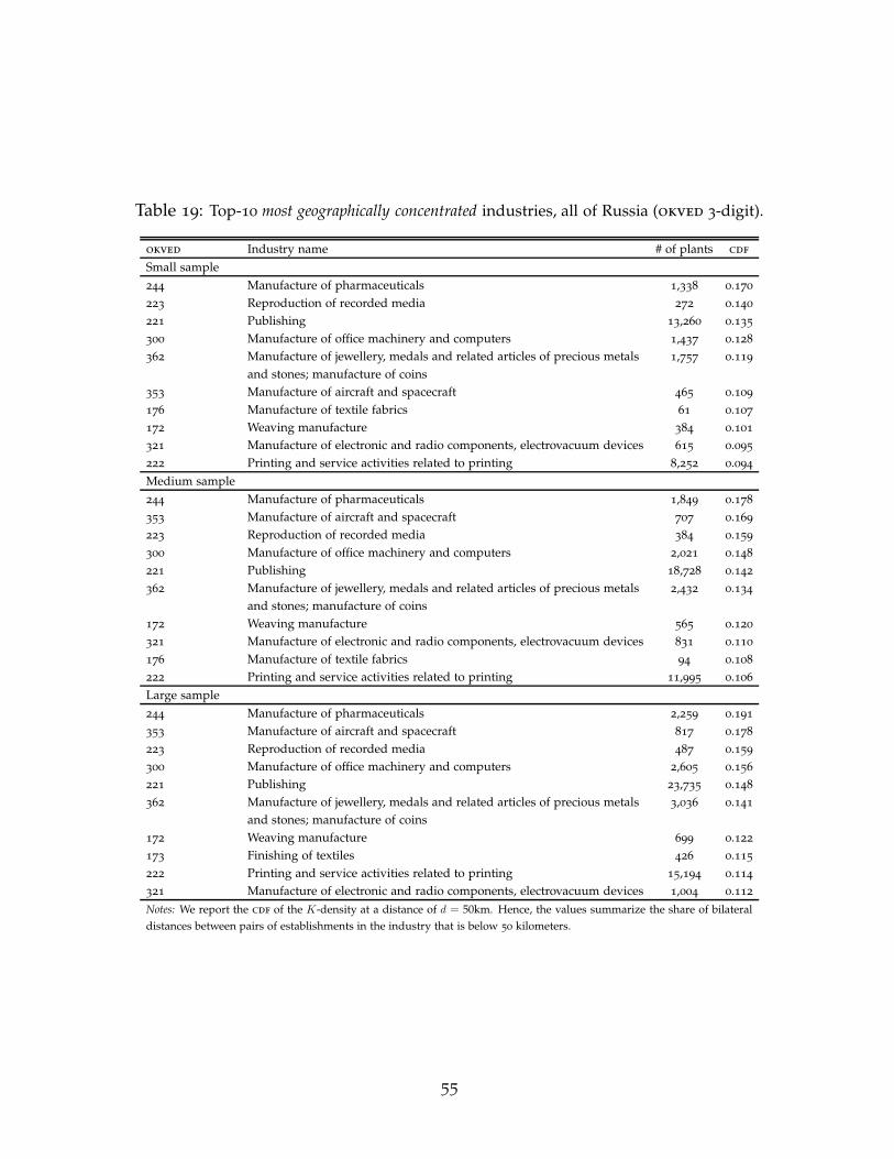
Table 19: Top-10 most geographically concentrated industries, all of Russia (okved 3-digit).
okved Industry name # of plants cdf
Small sample
244 Manufacture of pharmaceuticals 1,338 0.170
223 Reproduction of recorded media 272 0.140
221 Publishing 13,260 0.135
300 Manufacture of office machinery and computers 1,437 0.128
362 Manufacture of jewellery, medals and related articles of precious metals 1,757 0.119
and stones; manufacture of coins
353 Manufacture of aircraft and spacecraft 465 0.109
176 Manufacture of textile fabrics 61 0.107
172 Weaving manufacture 384 0.101
321 Manufacture of electronic and radio components, electrovacuum devices 615 0.095
222 Printing and service activities related to printing 8,252 0.094
Medium sample
244 Manufacture of pharmaceuticals 1,849 0.178
353 Manufacture of aircraft and spacecraft 707 0.169
223 Reproduction of recorded media 384 0.159
300 Manufacture of office machinery and computers 2,021 0.148
221 Publishing 18,728 0.142
362 Manufacture of jewellery, medals and related articles of precious metals 2,432 0.134
and stones; manufacture of coins
172 Weaving manufacture 565 0.120
321 Manufacture of electronic and radio components, electrovacuum devices 831 0.110
176 Manufacture of textile fabrics 94 0.108
222 Printing and service activities related to printing 11,995 0.106
Large sample
244 Manufacture of pharmaceuticals 2,259 0.191
353 Manufacture of aircraft and spacecraft 817 0.178
223 Reproduction of recorded media 487 0.159
300 Manufacture of office machinery and computers 2,605 0.156
221 Publishing 23,735 0.148
362 Manufacture of jewellery, medals and related articles of precious metals 3,036 0.141
and stones; manufacture of coins
172 Weaving manufacture 699 0.122
173 Finishing of textiles 426 0.115
222 Printing and service activities related to printing 15,194 0.114
321 Manufacture of electronic and radio components, electrovacuum devices 1,004 0.112
Notes: We report the cdf of the K-density at a distance of d = 50km. Hence, the values summarize the share of bilateral
distances between pairs of establishments in the industry that is below 50 kilometers.
55

Figure 15: Skewness of the strength of localization and K-density cdf (large sample, okved 3-digit).
(1) Western Russia. (2) Eastern Russia.
0.1
.2.3
Str
en
gth
of
loca
liza
tion
, cu
mu
lativ
e a
t 1
,00
0km
0 20 40 60 80 100Number of industries
0.0
5.1
.15
.2.2
5S
tre
ng
th o
f lo
caliz
atio
n,
cum
ula
tive
at
1,0
00
km
0 20 40 60 80 100Number of industries
.2.4
.6.8
1K
−d
en
sity
CD
F a
t 1
,00
0km
0 20 40 60 80 100Number of industries
.1.2
.3.4
.5.6
K−
de
nsi
ty C
DF
at
1,0
00
km
0 20 40 60 80 100Number of industries
56

Table 20: Top-10 least localized industries (okved 4-digit, large samples).
okved Industry name # of plants ΨA
All of Russia
1520 Processing and preserving of fish and fish products 2,549 0.149
3511 Building and repairing of ships 2,002 0.107
1598 Production of mineral waters and soft drinks 2,562 0.088
1596 Manufacture of beer 898 0.079
2212 Publishing of newspapers 4,457 0.070
2661 Manufacture of concrete products for construction purposes 5,473 0.070
1581 Manufacture of bread; manufacture of fresh pastry goods and cakes 7,170 0.060
2952 Manufacture of machinery for mining, quarrying and construction 961 0.049
2640 Manufacture of bricks, tiles and construction products, in baked clay 1,673 0.049
2411 Manufacture of industrial gases 595 0.044
Western Russia
1598 Production of mineral waters and soft drinks 1,877 0.102
1520 Processing and preserving of fish and fish products 1,633 0.085
1591 Manufacture of distilled potable alcoholic beverages 332 0.081
1596 Manufacture of beer 623 0.077
2663 Manufacture of ready-mixed concrete 1,679 0.060
2411 Manufacture of industrial gases 411 0.045
2320 Manufacture of refined petroleum products 1,330 0.039
3510 Building and repairing of ships and boats 310 0.035
3661 Manufacture of imitation jewellery 78 0.029
1532 Manufacture of fruit and vegetable juice 236 0.028
Eastern Russia
1598 Production of mineral waters and soft drinks 685 0.045
3622 Manufacture of jewellery and related articles of precious metals and stones 398 0.039
2411 Manufacture of industrial gases 184 0.027
2663 Manufacture of ready-mixed concrete 463 0.017
2221 Printing of newspapers 155 0.013
2210 Publishing 1,711 0.012
1596 Manufacture of beer 275 0.010
2661 Manufacture of concrete products for construction purposes 1,519 0.009
2911 Manufacture of engines and turbines, except aircraft, jet, vehicle and 186 0.007
cycles engines
2640 Manufacture of bricks, tiles and construction products, in baked clay 414 0.005
Notes: ΨA is computed at 990km, 995km and 999km (the last point at which the K-densities are evaluated) for the large,
the medium, and the small samples, respectively. We hence measure localization over the whole distance range that we
compute the K-densities for.
57

Table 21: Top-10 most dispersed industries (okved 3-digit, large sample).
okved Industry name # of plants cdf
All of Russia
152 Processing and preserving of fish and fish products 2,549 0.150
351 Building and repairing of ships and boats 2,710 0.089
159 Manufacture of beverages 4,642 0.081
266 Manufacture of articles of concrete, plaster or cement 12,380 0.062
151 Production, processing and preserving of meat and meat products 6,576 0.046
268 Manufacture of other non-metallic mineral products 2,233 0.024
283 Manufacture of steam generators, except central heating hoboilers; manufacture 667 0.024
of nuclear reactors
282 Manufacture of metal tanks, reservoirs and containers; manufacture of central 1,491 0.019
heating radiators and boilers
153 Processing and preserving of potato, fruit and vegetables 1,762 0.018
157 Manufacture of prepared animal feeds 1,141 0.015
Western Russia
159 Manufacture of beverages 3,510 0.108
152 Processing and preserving of fish and fish products 1,633 0.085
153 Processing and preserving of potato, fruit and vegetables 1,377 0.030
157 Manufacture of prepared animal feeds 873 0.029
333 Manufacture of industrial process control equipment 469 0.021
295 Manufacture of other special purpose machinery 3,842 0.002
265 Manufacture of cement, lime and plaster 433 0.001
160 Manufacture of tobacco products 98 0.000
335 Manufacture of watches and clocks and other time instruments 158 0.000
176 Manufacture of textile fabrics 106 0.000
Eastern Russia
152 Processing and preserving of fish and fish products 916 0.076
362 Manufacture of jewellery, medals and related articles of precious metals 435 0.045
and stones; manufacture of coins
159 Manufacture of beverages 1,132 0.041
266 Manufacture of articles of concrete, plaster or cement 3,218 0.013
232 Manufacture of refined petroleum products 282 0.007
264 Manufacture of bricks, tiles and construction products, in baked clay 414 0.006
341 Manufacture of motor vehicles 164 0.000
154 Manufacture of vegetable and animal oils and fats 227 0.000
275 Casting of metals 202 0.000
272 Manufacture of crude iron and steel pipes 97 0.000
Notes: We report the cdf of the K-density at a distance of d = 50km. Hence, the values summarize the share of bilateral
distances between pairs of establishments in the industry that is below 50 kilometers.
58

Table 22: Top 10 most localized industries, western Russia (okved 3-digit).
okved Industry name # of plants ΓA
Small sample
223 Reproduction of recorded media 247 0.359
244 Manufacture of pharmaceuticals 1,145 0.273
335 Manufacture of watches and clocks and other time instruments 97 0.238
172 Weaving manufacture 362 0.214
300 Manufacture of office machinery and computers 1,224 0.188
362 Manufacture of jewellery, medals and related articles of precious metals 1,514 0.187
and stones; manufacture of coins
173 Finishing of textiles 209 0.159
171 Spinning of textile fibres 251 0.156
353 Manufacture of aircraft and spacecraft 418 0.155
221 Publishing 10,730 0.148
Medium sample
223 Reproduction of recorded media 346 0.393
353 Manufacture of aircraft and spacecraft 644 0.269
244 Manufacture of pharmaceuticals 1,583 0.267
172 Weaving manufacture 533 0.264
176 Manufacture of textile fabrics 85 0.228
173 Finishing of textiles 293 0.227
362 Manufacture of jewellery, medals and related articles of precious metals 2,097 0.218
and stones; manufacture of coins
300 Manufacture of office machinery and computers 1,730 0.202
321 Manufacture of electronic and radio components, electrovacuum devices 741 0.161
171 Spinning of textile fibres 371 0.155
Large sample
223 Reproduction of recorded media 438 0.312
244 Manufacture of pharmaceuticals 1,943 0.270
353 Manufacture of aircraft and spacecraft 745 0.269
173 Finishing of textiles 373 0.248
172 Weaving manufacture 658 0.245
362 Manufacture of jewellery, medals and related articles of precious metals 2,601 0.223
and stones; manufacture of coins
300 Manufacture of office machinery and computers 2,220 0.203
176 Manufacture of textile fabrics 106 0.192
335 Manufacture of watches and clocks and other time instruments 158 0.155
221 Publishing 19,142 0.149
Notes: ΓA is computed at 990km, 995km and 999km (the last point at which the K-densities are evaluated) for the large,
the medium, and the small samples, respectively. We hence measure localization over the whole distance range that we
compute the K-densities for.
59

Table 23: Top 10 most localized industries, eastern Russia (okved 3-digit).
okved Industry name # of plants ΓA
Small sample
343 Manufacture of parts and accessories for motor vehicles and their engines 119 0.238
286 Manufacture of cutlery, tools and general hardware 102 0.163
156 Manufacture of grain mill products, starches and starch products 352 0.144
341 Manufacture of motor vehicles 99 0.136
272 Manufacture of crude iron and steel pipes 58 0.136
342 Manufacture of bodies (coachwork) for motor vehicles; manufacture of 53 0.116
trailers and semi-trailers
285 Treatment and coating of metals; general mechanical engineering 962 0.108
154 Manufacture of vegetable and animal oils and fats 128 0.098
294 Manufacture of machine-tools 262 0.094
271 Manufacture of crude iron, ferroalloy, steel 172 0.086
Medium sample
343 Manufacture of parts and accessories for motor vehicles and their engines 182 0.225
341 Manufacture of motor vehicles 142 0.192
271 Manufacture of crude iron, ferroalloy, steel 261 0.155
272 Manufacture of crude iron and steel pipes 82 0.136
283 Manufacture of steam generators, except central heating hoboilers; 190 0.126
manufacture of nuclear reactors
154 Manufacture of vegetable and animal oils and fats 190 0.109
285 Treatment and coating of metals; general mechanical engineering 1,399 0.107
156 Manufacture of grain mill products, starches and starch products 509 0.106
342 Manufacture of bodies (coachwork) for motor vehicles; manufacture of 77 0.105
trailers and semi-trailers
294 Manufacture of machine-tools 382 0.091
Large sample
341 Manufacture of motor vehicles 164 0.257
343 Manufacture of parts and accessories for motor vehicles and their engines 230 0.241
271 Manufacture of crude iron, ferroalloy, steel 314 0.167
272 Manufacture of crude iron and steel pipes 97 0.164
342 Manufacture of bodies (coachwork) for motor vehicles; manufacture of 90 0.142
trailers and semi-trailers
156 Manufacture of grain mill products, starches and starch products 597 0.117
285 Treatment and coating of metals; general mechanical engineering 1,764 0.115
275 Casting of metals 202 0.111
294 Manufacture of machine-tools 479 0.103
154 Manufacture of vegetable and animal oils and fats 227 0.099
Notes: ΓA is computed at 990km, 995km and 999km (the last point at which the K-densities are evaluated) for the large,
the medium, and the small samples, respectively. We hence measure localization over the whole distance range that we
compute the K-densities for.
60

Table 24: Top 10 most geographically concentrated industries, western Russia (okved 3-digit).
okved Industry name # of plants cdf
Small sample
244 Manufacture of pharmaceuticals 1,145 0.296
223 Reproduction of recorded media 247 0.292
221 Publishing 10,730 0.227
335 Manufacture of watches and clocks and other time instruments 97 0.223
300 Manufacture of office machinery and computers 1,224 0.187
362 Manufacture of jewellery, medals and related articles of precious metals 1,514 0.166
and stones; manufacture of coins
222 Printing and service activities related to printing 6,632 0.164
173 Finishing of textiles 209 0.149
353 Manufacture of aircraft and spacecraft 418 0.145
331 Manufacture of medical and surgical equipment and orthopaedic appliances 1,628 0.138
Medium sample
223 Reproduction of recorded media 346 0.355
244 Manufacture of pharmaceuticals 1,583 0.293
353 Manufacture of aircraft and spacecraft 644 0.263
221 Publishing 15,109 0.233
173 Finishing of textiles 293 0.219
300 Manufacture of office machinery and computers 1,730 0.213
362 Manufacture of jewellery, medals and related articles of precious metals 2,097 0.194
and stones; manufacture of coins
222 Printing and service activities related to printing 9,629 0.180
176 Manufacture of textile fabrics 85 0.159
331 Manufacture of medical and surgical equipment and orthopaedic appliances 2,337 0.152
Large sample
244 Manufacture of pharmaceuticals 1,943 0.307
223 Reproduction of recorded media 438 0.290
353 Manufacture of aircraft and spacecraft 745 0.274
173 Finishing of textiles 373 0.240
221 Publishing 19,142 0.238
300 Manufacture of office machinery and computers 2,220 0.229
362 Manufacture of jewellery, medals and related articles of precious metals 2,601 0.210
and stones; manufacture of coins
222 Printing and service activities related to printing 12,211 0.190
331 Manufacture of medical and surgical equipment and orthopaedic appliances 2,764 0.166
176 Manufacture of textile fabrics 106 0.162
Notes: We report the cdf of the K-density at a distance of d = 50km. Hence, the values summarize the share of bilateral
distances between pairs of establishments in the industry that is below 50 kilometers.
61

Table 25: Top 10 most geographically concentrated industries, eastern Russia (okved 3-digit).
okved Industry name # of plants cdf
Small sample
343 Manufacture of parts and accessories for motor vehicles and their engines 119 0.084
272 Manufacture of crude iron and steel pipes 58 0.064
286 Manufacture of cutlery, tools and general hardware 102 0.062
341 Manufacture of motor vehicles 99 0.059
285 Treatment and coating of metals; general mechanical engineering 962 0.055
342 Manufacture of bodies (coachwork) for motor vehicles; manufacture of 53 0.054
trailers and semi-trailers
154 Manufacture of vegetable and animal oils and fats 128 0.052
271 Manufacture of crude iron, ferroalloy, steel 172 0.051
294 Manufacture of machine-tools 262 0.051
283 Manufacture of steam generators, except central heating hoboilers; 139 0.049
manufacture of nuclear reactors
Medium sample
343 Manufacture of parts and accessories for motor vehicles and their engines 182 0.092
341 Manufacture of motor vehicles 142 0.079
271 Manufacture of crude iron, ferroalloy, steel 261 0.068
272 Manufacture of crude iron and steel pipes 82 0.067
283 Manufacture of steam generators, except central heating hoboilers; 190 0.060
manufacture of nuclear reactors
285 Treatment and coating of metals; general mechanical engineering 1,399 0.058
294 Manufacture of machine-tools 382 0.054
342 Manufacture of bodies (coachwork) for motor vehicles; manufacture of 77 0.054
trailers and semi-trailers
154 Manufacture of vegetable and animal oils and fats 190 0.053
275 Casting of metals 158 0.049
Large sample
341 Manufacture of motor vehicles 164 0.100
343 Manufacture of parts and accessories for motor vehicles and their engines 230 0.095
272 Manufacture of crude iron and steel pipes 97 0.070
271 Manufacture of crude iron, ferroalloy, steel 314 0.069
351 Building and repairing of ships and boats 619 0.061
285 Treatment and coating of metals; general mechanical engineering 1,764 0.059
342 Manufacture of bodies (coachwork) for motor vehicles; manufacture of 90 0.059
trailers and semi-trailers
294 Manufacture of machine-tools 479 0.056
274 Manufacture of non-ferrous metals 269 0.054
154 Manufacture of vegetable and animal oils and fats 227 0.052
Notes: We report the cdf of the K-density at a distance of d = 50km. Hence, the values summarize the share of bilateral
distances between pairs of establishments in the industry that is below 50 kilometers.
62