
Manual: Portable Chlorophyll Fluorometer PAM-2500 of the well-known PAM-2000/2100 instruments which...
112
Portable Chlorophyll Fluorometer PAM-2500 Handbook of Operation 2.156/08.2008 1. (preliminary) Edition: August 2008 PAM_2500_03pp.doc © Heinz Walz GmbH, 2008 Heinz Walz GmbH • Eichenring 6 • 91090 Effeltrich • Germany Phone +49-(0)9133/7765-0 • Telefax +49-(0)9133/5395 E-mail [email protected] • Internet www.walz.com
-
Upload
truonghanh -
Category
Documents
-
view
231 -
download
2
Transcript of Manual: Portable Chlorophyll Fluorometer PAM-2500 of the well-known PAM-2000/2100 instruments which...

Portable Chlorophyll Fluorometer
PAM-2500 Handbook of Operation
2.156/08.2008 1. (preliminary) Edition: August 2008
PAM_2500_03pp.doc
© Heinz Walz GmbH, 2008
Heinz Walz GmbH • Eichenring 6 • 91090 Effeltrich • Germany Phone +49-(0)9133/7765-0 • Telefax +49-(0)9133/5395
E-mail [email protected] • Internet www.walz.com

CONTENTS
Contents
1 Safety Instructions ....................................................................... 7 1.1 General Safety Instructions ......................................................... 7 1.2 Special Safety Instructions.......................................................... 7
2 Introduction .................................................................................. 9 2.1 Intention of this Handbook ....................................................... 10
3 Components and Setup .............................................................. 11 3.1 Basic System Components ........................................................ 11 3.2 Basic System Setup ................................................................... 11 3.3 PamWin-3 Software Installation ............................................... 13
3.3.1 USB Serial Port Setting .................................................... 14 3.3.2 Wireless Bluetooth Communication ................................. 15
3.4 Accessories................................................................................ 16 3.4.1 Field Combo (optional)..................................................... 16
3.4.1.1 Touch-Screen Ultra-Mobile Personal Computer ............ 16 3.4.1.2 External Battery 000160101314 ..................................... 16 3.4.1.3 Automatic Charger 0001X.............................................. 17
3.4.2 Additional Components .................................................... 18 3.4.2.1 Special Fiberoptics 2010-F ............................................. 18 3.4.2.2 Distance Clip 60° 2010-A............................................... 18 3.4.2.3 Leaf-Clip Holder 2030-B (optional) ............................... 20 3.4.2.4 Micro Quantum/Temp.-Sensor 2060-M (optional)......... 23 3.4.2.5 Dark Leaf Clip DLC-8 (optional) ................................... 23
4 PAM-2500 Operation................................................................. 25 4.1 PamWin-3 Help......................................................................... 25 4.2 Field Screen............................................................................... 25
4.2.1 Monitoring Graphs............................................................ 26
1
CONTENTS
4.2.2 Program and Script Control .............................................. 27 4.2.3 Alphanumerical Area........................................................ 27
4.2.3.1 Light Control .................................................................. 29 4.2.3.2 Fluorescence Data........................................................... 32 4.2.3.3 Fluorescence Ratio Parameters ....................................... 33 4.2.3.4 Additional Data............................................................... 35
4.2.4 First Measurements Using the Field Screen ..................... 36 4.3 PamWin-3: Advanced Level ..................................................... 38
4.3.1 General Settings................................................................ 38 4.3.1.1 Menu Bar ........................................................................ 38 4.3.1.2 Measuring Light Frequency............................................ 45 4.3.1.3 Induction Curve Parameters............................................ 45 4.3.1.4 Global Settings ............................................................... 46 4.3.1.5 PAR Sensor Control ....................................................... 47 4.3.1.6 Fo, Fo’ ............................................................................ 47 4.3.1.7 Tab Bar ........................................................................... 48 4.3.1.8 Pulses, Short Term Illumination ..................................... 48 4.3.1.9 Mode............................................................................... 50 4.3.1.10 Clock Event ............................................................... 50 4.3.1.11 New Record ............................................................... 51
4.4 SP-Analysis Mode .................................................................... 52 4.4.1 Slow Kinetics Window ..................................................... 52
4.4.1.1 Graph Icons..................................................................... 53 4.4.1.2 Graph Y, X ..................................................................... 53 4.4.1.3 Save Ft ............................................................................ 53 4.4.1.4 Display Control............................................................... 53 4.4.1.5 X-Axis Scaling/Zoom In................................................. 54 4.4.1.6 Slow Kinetics Control..................................................... 54
2
CONTENTS
4.4.2 Light Curve ....................................................................... 55 4.4.2.1 Display Control............................................................... 55 4.4.2.2 LC (Light Curve) Control ............................................... 56 4.4.2.3 Light Curve Edit ............................................................. 57 4.4.2.4 Light Curve Fit................................................................ 57
4.4.3 Report................................................................................ 58 4.4.3.1 Report Data Management ............................................... 58 4.4.3.2 Record Header and Last Line ......................................... 60 4.4.3.3 Record Columns ............................................................. 61
4.5 Fast Acquisition Mode .............................................................. 62 4.5.1 Fast Settings...................................................................... 62
4.5.1.1 Basic Settings.................................................................. 63 4.5.1.2 Menu Bar ........................................................................ 64 4.5.1.3 Trigger Settings ( I ) and ( II ) ........................................ 64 4.5.1.4 Light & Pulses ................................................................ 69 4.5.1.5 Start Fast Kinetics ........................................................... 70
4.5.2 Fast Kinetics ..................................................................... 70 4.5.2.1 Cursor Coordinates ......................................................... 71 4.5.2.2 File Names ...................................................................... 71 4.5.2.3 File Menu........................................................................ 72 4.5.2.4 Fast Kinetics ................................................................... 72 4.5.2.5 Polyphasic Fluorescence Rise......................................... 74
4.6 View Mode................................................................................ 74 4.6.1 Icon Bar............................................................................. 76 4.6.2 Sidebar .............................................................................. 76 4.6.3 Pick Data........................................................................... 76
4.7 Script Files ................................................................................ 76 5 Definitions and Equations ......................................................... 79
3
CONTENTS
5.1 Relative Fluorescence Yields.................................................... 79 5.1.1 Measurements with dark-acclimated samples................... 79 5.1.2 Measurements with light-exposed (treated) samples ........ 79
5.2 Fluorescence Ratio Parameters ................................................. 80 5.3 Constant Fraction of Fo Fluorescence (C/Fo)........................... 84 5.4 Relative Electron Transfer Rate (ETR)..................................... 85 5.5 Rapid Light Curves ................................................................... 87
5.5.1 Some Papers on Rapid Light Curves ................................ 89 5.6 Literature Cited in Chapter 5 .................................................... 90
6 Some Reviews on Chlorophyll Fluorescence ........................... 93 7 Specifications .............................................................................. 95
7.1 Basic System............................................................................. 95 7.1.1 General Design ................................................................. 95 7.1.2 Light sources..................................................................... 96 7.1.3 Special Fiberoptics 2010-F ............................................... 96 7.1.4 Distance Clip 60° 2010-A................................................. 97 7.1.5 Battery Charger MINI-PAM/L ......................................... 97 7.1.6 External Voltage Supply Cable ........................................ 97 7.1.7 System Control and Data Acquisition .............................. 97 7.1.8 Carrier Bag........................................................................ 98 7.1.9 Transport Box 2040-T ...................................................... 98 7.1.10 Minimum Computer Requirements .................................. 98
7.2 Accessories ............................................................................... 99 7.2.1 Ultra-Mobile Personal Computer for Field Research ....... 99
7.2.1.1 Computer box ................................................................. 99 7.2.1.2 Ultra-mobile touchscreen computer SAMSUNG Q1 Ultra
99 7.2.2 External battery 000160101314...................................... 100
4

CONTENTS
7.2.3 Automatic charger 000190101099.................................. 100 7.2.4 Leaf-Clip Holder 2030-B................................................ 100 7.2.5 Arabidopsis Leaf Clip 2060-B ........................................ 100 7.2.6 Dark Leaf Clip DLC-8 .................................................... 101 7.2.7 Micro Quantum/Temperature-Sensor 2060-M ............... 101 7.2.8 Suspension Cuvette KS-2500 ......................................... 101 7.2.9 Magnetic Stirrer MKS-2500 ........................................... 102 7.2.10 Compact Tripod ST-2101A ............................................ 102
8 Trouble Shooting...................................................................... 103 9 Warranty................................................................................... 105
9.1 Conditions ............................................................................... 105 9.2 Instructions.............................................................................. 106
10 Index.......................................................................................... 107
5


SAFETY INSTRUCTIONS CHAPTER 1
1 Safety Instructions
1.1 General Safety Instructions a ) Read the safety instructions and the operating instructions
first.
b ) Pay attention to all the safety warnings.
c ) Keep the device away from water or high moisture areas.
d ) Keep the device away from dust, sand and dirt.
e ) Always ensure there is sufficient ventilation.
f ) Do not put the device anywhere near sources of heat.
g ) Connect the device only to the power source indicated in the operating instructions or on the device.
h ) Clean the device only according to the manufacturer’s rec-ommendations.
i ) If the device is not in use, remove the mains plug from the socket.
j ) Ensure that no liquids or other foreign bodies can find their way inside the device.
k ) The device should only be repaired by qualified personnel.
1.2 Special Safety Instructions The PAM-2500 is a highly sensitive instrument which should be only used for research purposes, as specified in this manual. Follow the instructions of this manual in order to avoid potential harm to the user and damage to the instrument.
The PAM-2500 can emit very strong light! In order to avoid harm to your eyes, never look directly at the fiberoptics end, or at open light ports at the front side of the control unit.
7


INTRODUCTION CHAPTER 2
2 Introduction
The PAM-2500 Portable Chlorophyll Fluorometer is the follow-up model of the well-known PAM-2000/2100 instruments which were introduced in the 1990s as the first portable PAM fluorometers and since then have been successfully applied worldwide by numerous scientists. In the development of the PAM-2500, particular care was taken to maintain all properties appreciated by PAM-2000/2100 users and, at the same time, to take account of the recent technical pro-gress.
Essentially, the hardware and optical system are thoroughly modern-ized. Also, while continuing basic elements of the graphical user in-terface, instrument operation is based on the newly-developed Pam-Win-3 software. The program permits operation under Windows op-erating systems on normal personal computers, but also on ultra mo-bile touch screen computers.
Major points of progress of the PAM-2500 with respect to its prede-cessors are:
- Use of LEDs (light emitting diodes) for all internal light sources including Saturation Pulses and Actinic Light.
- Blue and Red Actinic internal light sources.
- Single turn-over and multiple turn-over saturating flashes.
- Time resolution down to 10 µs.
- Easily updateable firmware.
- Optional touch-screen operation by an ultra-mobile com-puter.
9

CHAPTER 2 INTRODUCTION
2.1 Intention of this Handbook The Portable Fluorometer PAM-2500 displays a high degree of flexi-bility in measuring and analyzing fluorescence. This does not mean, however, that all features of this multifunctional instrument must be understood before measurements can be started. Actually, due to the "intelligent" central control of all functions by the special PamWin-3 software, serious operational mistakes harming the instrument are highly unlikely. Also, at first there is no need to care about the nu-merous settings of instrument parameters, because these are pre-adjusted for standard measurements. Hence, even the inexperienced user can start measuring with a minimum of background knowledge, and will be gradually guided to deeper understanding and more pro-found applications.
This handbook tries to cover all of the numerous features and appli-cations of the PAM-2500 Fluorometer, some of which probably are not of immediate interest to many users, but probably will become relevant, as new questions arise on the basis of the results obtained. The best way to become acquainted with all features of the PAM-2500 Fluorometer is to read this handbook section by section, trying out all described functions. On the other hand, in order to get a quick start it will suffice to read Chapter 4.2.
10

COMPONENTS & SETUP CHAPTER 3
3 Components and Setup
3.1 Basic System Components The basic system consists of the following components:
a ) PAM-2500 Control Unit
b ) Special Fiberoptics 2010-F
c ) Distance Clip 60° 2010-A
d ) Battery Charger MINI-PAM/L
e ) MINI-PAM/AK cable
f ) Special USB cable PAM-2500/K1
g ) Fluorescence Standard Foil
h ) Spare Fuse
i ) Carrier Bag
j ) Transport Box 2040-T
k ) Software. PamWin-3 System Control and Data Acquisition
3.2 Basic System Setup
Note: Great caution should be exercised to prevent any dirt or for-eign matter from entering the ports for the fiberoptics pins.
To set up the PAM-2500 fluorometer:
- Connect fiberoptics to the control unit using the three-pin op-tical connector at the front of the unit (Fig. 3.1).
11
CHAPTER 3 COMPONENTS & SETUP
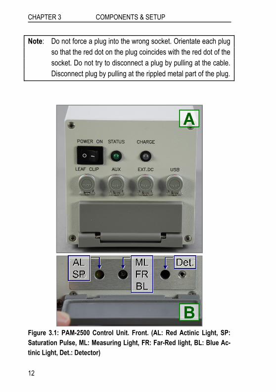
Note: Do not force a plug into the wrong socket. Orientate each plug so that the red dot on the plug coincides with the red dot of the socket. Do not try to disconnect a plug by pulling at the cable. Disconnect plug by pulling at the rippled metal part of the plug.
Figure 3.1: PAM-2500 Control Unit. Front. (AL: Red Actinic Light, SP: Saturation Pulse, ML: Measuring Light, FR: Far-Red light, BL: Blue Ac-tinic Light, Det.: Detector)
12
COMPONENTS & SETUP CHAPTER 3
- Connect the battery charger cable to the <EXT.DC> socket (Fig. 3.1 A), and to line power: thereafter, a green <CHARGE> LED (Fig. 3.1 A) indicates that the internal bat-tery is charged but yellow LED light signifies that the battery is currently charged. Please note that an external 12 V battery cannot recharge the internal battery; but it can provide power (via the MINI-PAM/AK cable) when the internal battery is empty.
- Connect computer and control unit (USB socket, Fig. 3.1 A) by the PAM-2500 special USB cable.
- Switch on PAM-2500 using the toggle switch labeled POWER ON (Fig. 3.1 A). Flashing of the <Status LED> (Fig. 3.1 A) indicates that the system is ready for communi-cations. The LED will shine continuously once communica-tion with the computer has been established. Constant light from the <Status LED> in the absence of computer commu-nication indicates malfunction of the PAM-2500. Usually, switching power OFF and, after a couple of seconds, ON again will restore normal function.
3.3 PamWin-3 Software Installation Depending on the type of CD-ROM delivered with the PAM-2500 Chlorophyll Fluorometer, you have to start installation with a) or b).
a) Your <Software & Manuals CD-ROM> contains only a setup file (e. g. <PamWin_setup.exe>), and the present handbook in PDF file format.
- Close other programs before installation of the PamWin_3 software.
13
CHAPTER 3 COMPONENTS & SETUP
- Double click on the setup file and follow instructions. The setup routine will create in the <C:> root directory the folder <PamWin_3> containing the PamWin-3 main program and accessory files. Further, an icon representing a shortcut to PamWin-3 is created on the computer desktop.
b) Your <Software & Manuals CD-ROM> contains the com-plete collection of the Walz Software & Manuals.
- The CD automatically starts the default internet browser of your computer. (If automatic browser start fails, double-click on <index.html> in the root directory of the <Software & Manuals> CD-ROM.)
- Choose <Fluorescence Products> → <PAM-2500> → <PC software PamWin-3>.
- Close other programs before installation of the PamWin_3 software.
- Click on <PamWin-3> to start software installation as de-scribed above.
3.3.1 USB Serial Port Setting For serial communication via a serial USB port, a driver software is installed during the PamWin-3 setup procedure. The successful driver installation will be confirmed by the software. At first start of the PamWin-3 software, the program checks the setting of the “la-tency timer” which needs to be adjusted to 1 ms to ensure high rates of data transfer.
The latency timer is set to 1 ms on the port (COM & LPT) properties page which is accessed via the device manager. For Windows XP computers proceed as described below (the procedure is similar for the Windows Vista operating system):
14

COMPONENTS & SETUP CHAPTER 3
- Make sure that the PAM-2500 is switched on and connected by the USB cable to the computer
- Open <Windows Start Menu>
- Select <Settings>
- Select <Control Panel>
- Select <System> and left-click the <Hardware> tab
- Left-click the <Device Manager> button
- Open folder <Ports & LPT>
- Select <USB Serial Port COM#> (double click with left mouse key).
- Select <Port Settings> tab with left mouse key
- Left-click the <Advanced> button
- Set latency timer to 1 ms
- Close by clicking <OK> in the <Advanced Settings> win-dow, and the <USB properties> window
3.3.2 Wireless Bluetooth Communication - Please note that Bluetooth data transfer is too slow for the
<Fast Kinetics> mode of PamWin-3. The <Fast Kinetics> mode is not available when in Bluetooth communication is active.
- Make sure that the PAM-2500 is switched on and NOT con-nected via USB cable to a computer.
- Open <My Bluetooth Places> in the <Start> menu or on the computer desktop.
- Start by double-click <Find Bluetooth devices>
15
CHAPTER 3 COMPONENTS & SETUP
- Now, the device <PAM 2500 SNR XXXX> should be in the list of Bluetooth devices (the four “X” stand for the four digit serial number). If the PAM 2500 is not listed, change posi-tions of PAM 2500 relative to computer. (Hint: the Bluetooth output antenna is located at the rear top face of the PAM 2500 instrument.)
- Double click on <PAM 2500 SNR XXXX> and, subse-quently on <SerialPort on PAM 2500 SNR XXXX>
- Now you’ll be prompted to enter a <Bluetooth security code> which is for all PAM 2500 chlorophyll fluorometers the number:
2500
- The Bluetooth connection is now ready for use.
3.4 Accessories See Chapter 7 for specifications of accessories.
3.4.1 Field Combo (optional) The add-ons summarized as <Field Combo> convert the PAM-2500 chlorophyll fluorometer into a highly mobile field station, equipped with the options that a normal PC offers and working for hours inde-pendent of line current.
3.4.1.1 Touch-Screen Ultra-Mobile Personal Computer
3.4.1.2 External Battery 000160101314
16
COMPONENTS & SETUP CHAPTER 3
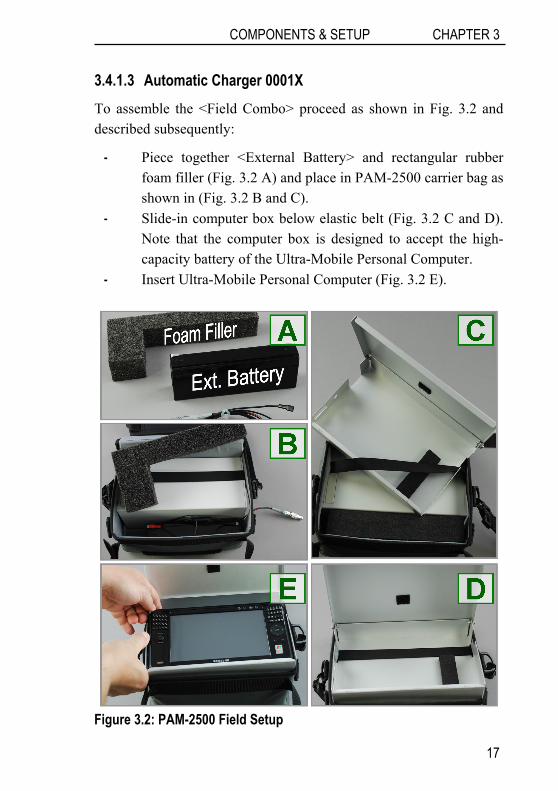
3.4.1.3 Automatic Charger 0001X To assemble the <Field Combo> proceed as shown in Fig. 3.2 and described subsequently:
- Piece together <External Battery> and rectangular rubber foam filler (Fig. 3.2 A) and place in PAM-2500 carrier bag as shown in (Fig. 3.2 B and C).
- Slide-in computer box below elastic belt (Fig. 3.2 C and D). Note that the computer box is designed to accept the high-capacity battery of the Ultra-Mobile Personal Computer.
- Insert Ultra-Mobile Personal Computer (Fig. 3.2 E).
Figure 3.2: PAM-2500 Field Setup
17

CHAPTER 3 COMPONENTS & SETUP
3.4.2 Additional Components
3.4.2.1 Special Fiberoptics 2010-F The Special Fiberoptics 2010-F are connected to the front side of the PAM-2500 control unit with the help of a special plug that resembles an electrical connector. There are three "fiber pins" with different op-tical cross-sections, which fit into the corresponding holes at the front side of the PAM-2500 housing, where they interface the various light sources and the photodiode detector. Within the "interface plug" the three fiber branches are joint to a common fiber bundle and random-ized via a 100 cm mixing pathway.
Note: The fiberoptics should be handled with care. Excessive bend-ing, in particular close to the connector plug, should be avoided, as it would lead to fiber breakage resulting in a loss of signal amplitude. The fibers are protected by a steel-spiral and plastic mantle, which provide a natural resistance to strong bending.
3.4.2.2 Distance Clip 60° 2010-A A Distance Clip is provided with the fiberoptics for convenient posi-tioning of the fiberoptics end-piece relative to the sample. The axis of the end-piece is positioned at a 60° angle relative to the sample plane (angle of incidence, 30°). Minimum shading of the sample is achieved when the fiberoptics points towards the sample from the side opposite to incident light. Two spacer rings may be used to de-fine fixed distances.
The sample may be placed either below the hole (e. g. thick leaves, lichens and mosses) or, preferentially with normal leaves, above the
18

COMPONENTS & SETUP CHAPTER 3
hole (compare Fig. 3.3). In the latter case, the leaf can be held be-tween the folded part of the clip.
Figure 3.3: Distance Clip (to position leaf with respect to fiberoptics)
The distance between fiberoptics exit plane and sample has consider-able influence on signal amplitude and effective light intensities (Fig. 3.4). Clearly, with a 60° angle between sample plane and fiberoptics, the distance between fiber optics tip and leaf surface varies, and, hence, the leaf surface is exposed to slightly heterogeneous light in-tensities. A much more pronounced intensity gradient exists inside the leaf due to shading by the top chloroplast layers. In essence, the measured signal will be dominated by that part of the leaf which re-
Figure 3.4: Relationship between signal amplitude/light intensity and distance between fiberoptics exit plane and sample
19

CHAPTER 3 COMPONENTS & SETUP
ceives maximal intensity, as this also is most strongly excited by the Measuring Light and emits most of the fluorescence which is re-ceived by the fiberoptics.
3.4.2.3 Leaf-Clip Holder 2030-B (optional) The Leaf-Clip Holder 2030-B is connected to the <LEAF CLIP> socket (Fig. 3.1 A) for recording of PAR and temperature in parallel with chlorophyll fluorescence.
The Leaf-Clip Holder 2030-B is almost indispensable for field inves-tigations, when ambient light and temperature conditions may vary considerably. It substitutes for the standard "Distance Clip" as a de-vice for defined positioning of the fiberoptics relative to the leaf plane. It features special micro-quantum and temperature sensors, the readings of which are transferred to the PAM-2500 with every Satu-ration Pulse measurement.
Figure 3.5: Leaf-Clip Holder 2030-B with Fiberoptics 2010- F.
20

COMPONENTS & SETUP CHAPTER 3
In this holder, the leaf is resting on a Perspex tube with widened crest, which can be vertically adjusted, to account for different leaf thicknesses. The fiberoptics axis forms a 60° angle with the leaf plane. Optionally, a 90° fiberoptics adapter (2030-B90) is available. The distance between fiberoptics and leaf can be varied. Standard distances are defined by spacer rings. The illuminated leaf area is limited by a steel ring with 10 mm ∅ opening.
At the bottom of the Leaf-Clip Holder 2030-B, a tripod mounting thread is provided. Mounting the device on a tripod (e. g. Compact Tripod ST-2101) facilitates long term measurements with the same plant.
The handle of the Leaf-Clip Holder 2030-B features a red push-button for remote control of the PAM-2500. Pressing this button ini-tiated a Saturation Pulse.
Micro-Quantum-Sensor
A micro quantum sensor is integrated into the Leaf-Clip Holder 2030-B to monitor the photosynthetic active radiation (PAR) to which the sample is exposed. The micro-quantum-sensor measures incident PAR in µmol quanta/(m2·s), i.e. in units of flux density. Hence, the measured parameter PAR is identical to PPFD (photosyn-thetic photon flux density).
Essential optoelectronic elements of this micro-quantum-sensor are:
- a 1.5 mm ∅ diffusing disk - a 0.5 mm diameter fiber guiding the scattered light to the de-
tector - a filter combination selecting the photosynthetic active wave-
length range between 380 and 710 nm - a blue-enhanced silicon photodiode
21
CHAPTER 3 COMPONENTS & SETUP
The sensor is factory calibrated against a standard lamp. Radiation of the standard lamp approached the sensor surface perpendicularly, that is at an angle of incidence of 0°. Therefore, the 2030-B sensor meas-ures with adequate accuracy collimated light incident at low angles, but also completely diffuse radiation. The angular response of the sensor, however, deviates from the ideal cosine behavior: to be exact, the sensor overvalues collimated light impinging at greater angles of incidence. Therefore, when the PAM-2500 internal Actinic Light sources are applied via the fiberoptics (Fig. 3.5), e.g. for recording of light response curves, the sensor should be switched off via software (see Advanced Mode, General Settings, Section 4.3.1) and the PAR should be derived from previously defined PAR-lists (see Section 4.3.3.1).
The stability of calibration depends on keeping the diffuser clean. It is advisable to check calibration regularly by comparison with a stan-dard quantum sensor. Any deviation can be corrected by entering a recalibration factor in the PamWin-3 program (see Section 4.3.1.1). A substantial increase of the calibration factor from its original value of 1.000 indicates dirt-deposition on the diffuser, which may be re-versed by gentle cleaning using a cotton tip applicator, moistened with some ethanol.
Thermocouple Monitoring Leaf Temperature
A NiCr-Ni thermocouple is mounted in the Perspex tube on which the investigated leaf area is resting. Its tip is forming a loop that gen-tly presses against the lower surface of the leaf. In this way there is effective temperature equilibration and the thermocouple is protected from direct sun radiation. The reference couple is located on the cir-cuit board, in close proximity to the thermovoltage amplifier, en-closed in the bottom part of the holder. The relationship between thermovoltage and temperature is almost linear. With decreasing temperatures there is a small decline of ΔV/°C. Calibration was per-
22
COMPONENTS & SETUP CHAPTER 3
formed at 25 °C. At 0 °C or –15 °C the deviation amounts to 0.5 or 0.8 °C, respectively. An offset value can be entered in the PamWin-3 program (see Section 4.3.1.1).
The temperature, as well as the PAR data, is automatically stored in the Report-file after every saturation pulse, together with the on-line calculated quenching parameters.
3.4.2.4 Micro Quantum/Temp.-Sensor 2060-M (optional) The Micro Quantum/Temp.-Sensor 2060-M essentially displays the same features as outlined above for the Leaf-Clip Holder 2030-B, ex-cept that the micro-sensors of PAR and temperature are not mounted in a leaf-clip. This device is rather designed for experiments with ob-jects which are not leaf-shaped, like crustose lichens and cushions of moss. The two miniature sensors can be attached to the site where fluorescence is monitored without interfering with the actual meas-urement. A defined position with respect to the object and the fiber-optics exit plane can be achieved with the help of a special holder, in analogy to the "Distance Clip" (see above).
It should be pointed out that the sensitivity of the micro quantum sen-sor is affected by bending the relatively long, flexible light guide that bridges the distance between the small diffusing disk at the object and the detector in the metal housing. Therefore, this device cannot substitute for a reliable quantum sensor. Recalibration is recom-mended after bringing the sensor and the metal housing into a fixed position with respect to the object.
3.4.2.5 Dark Leaf Clip DLC-8 (optional) The Dark Leaf Clip DLC-8 weighs approx. 4 g and, hence, can be at-tached to most types of leaves without any detrimental effects. It is equipped with a miniature sliding shutter which prevents light access
23

CHAPTER 3 COMPONENTS & SETUP
to the leaf during a dark-adaptation period. This shutter is opened for the actual measurement only, when exposure to external light is pre-vented by the fiberoptics. Proper dark-acclimation is essential for de-termination of the maximal quantum yield Fv/Fm and for recording of dark-light induction kinetics.
Figure 3.6: Dark Leaf Clip
Using the Dark Leaf Clip DLC-8, the fiberoptics is positioned at right angle with respect to the leaf surface at the relatively short distance of 7 mm. As a consequence, signal amplitude is distinctly higher than when the Leaf-Clip Holder 2030-B with 60° fiberoptics angle is used. In order to avoid signal saturation, the settings of Measuring Light Intensity and Gain have to be correspondingly lowered with respect to the standard settings (see Section 4.2).
When the shutter is still closed and the Measuring Light is on, an arti-factual Ft signal is observed. This signal is due to a small fraction of the Measuring Light which is reflected from the closed shutter to the photodetector. However, this background signal is of no concern as the reflection is much smaller when the shutter is opened and the Measuring Light hits the strongly absorbing leaf instead of the metal surface of the shutter that acts like a mirror.
24
PAMWIN-3 FIELD SCREEN CHAPTER 4
4 PAM-2500 Operation
4.1 PamWin-3 Help All program levels of the PamWin-3 software offer online Help-texts with information on essentially all active user surface elements. To access the online Help-texts:
- Move mouse cursor on the window element of interest until a small tag (“Tooltip”) appears.
- A “Tooltip” remains visible for 2.5 seconds. During this inter-val, pressing the <@> or <F1> key results in the display of the relevant Help-text.
For getting acquainted with the instrument and its software, it is strongly recommended to make frequent use of this function.
4.2 Field Screen The <Field Screen> of the PamWin-3 software has been developed for outdoor operation of the PAM-2500 fluorometer where ease and simplicity of instrument control is important. Conveniently, the ele-ments of the <Field Screen> are accessible via the display of a touch screen PC. The <Field Screen> is divided into three areas containing (1) alphanumeric fields, (2) program and Script control, and (3) monitoring graphs, respectively (see Fig. 4.1).
The alphanumeric area contains the switches for light control and data derived from Saturation Pulse analysis. It also includes the Zoom In button: the <Zoom In> command results in the screen display of the alphanumeric area.
25

CHAPTER 4 PAMWIN-3 FIELD SCREEN
4.2.1 Monitoring Graphs The <Field Screen> provides 2 monitoring graphs (Fig. 4.1): the left graph records slow fluorescence changes, and also depicts Fm and Fm’ values as small crosses. Generally, only those Saturation Pulse analyses which result in graphical display of Fm or Fm’ values are entered in the Report file - Saturation Pulses analyses carried out with stopped monitoring screen are not reported. To view the Report file click the Report icon. Editing of the Report is restricted to the <Advanced> level of the PamWin-3 program.
Monitoring of slow kinetics begins automatically with PamWin-3 program start. The slow kinetics monitoring graph is restarted by an <Fo, Fm> determination via Fv/Fm (see below) or via the Stop / Start button. An Fv/Fm determination automatically adapts the Y axis range of both monitoring screens to the signal amplitude. The actual signal size (in Volts) can be read from the Y-axes. In both
Figure 4.1: Field Screen Overview.
26
PAMWIN-3 FIELD SCREEN CHAPTER 4
screens, the Fo and Fm levels are displayed as yellow and red dashed line, respectively. Always, the time axis of the slow kinetics monitor-ing screen covers an interval of 5 minutes which is automatically shifted to the left for monitoring times > 5 minutes. The right monitoring graph displays the fast fluorescence kinetics in-duced by last Saturation Pulse over a time interval of 1.6 seconds. In addition to the Fo and Fm lines, the determined Fm’ level is depicted as a dashed black line.
4.2.2 Program and Script Control The Program and Script Control section (Fig. 4.1) includes buttons to quit the program ( Exit PamWin ), to access to the full range of PamWin-3 capabilities ( Advanced ), and to load Script files which carry out automatically preprogrammed experimental protocols (Script: Load and Run ).
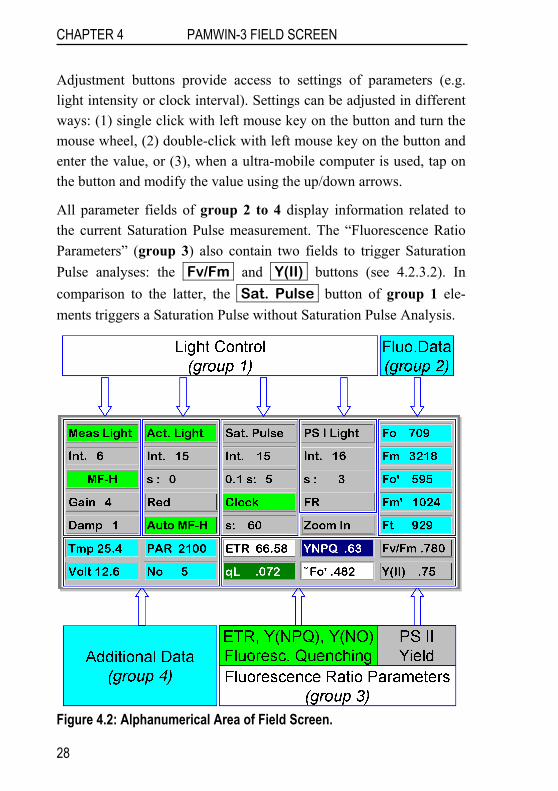
4.2.3 Alphanumerical Area The elements of the alphanumerical area are divided into four groups: (1) light control, (2) primary fluorescence data, (3) fluorescence ratio parameters, and (4) additional data like PAR and temperature (Fig. 4.2).
Group 1 (Light Control, see Fig. 4.2) includes “status” and “adjust-ment” buttons. A status button either turns on or off a function (e.g. the Measuring Light) or it changes the light color (e.g. red to blue Actinic Light). To change a status, click on the status button with the left mouse key. Status buttons with on/off-switching function display green background when the associated function is active. The status buttons controlling light color, display the selected type of light as text information.
27
CHAPTER 4 PAMWIN-3 FIELD SCREEN
Adjustment buttons provide access to settings of parameters (e.g. light intensity or clock interval). Settings can be adjusted in different ways: (1) single click with left mouse key on the button and turn the mouse wheel, (2) double-click with left mouse key on the button and enter the value, or (3), when a ultra-mobile computer is used, tap on the button and modify the value using the up/down arrows.
All parameter fields of group 2 to 4 display information related to the current Saturation Pulse measurement. The “Fluorescence Ratio Parameters” (group 3) also contain two fields to trigger Saturation Pulse analyses: the Fv/Fm and Y(II) buttons (see 4.2.3.2). In comparison to the latter, the Sat. Pulse button of group 1 ele-ments triggers a Saturation Pulse without Saturation Pulse Analysis.
Figure 4.2: Alphanumerical Area of Field Screen.
28

PAMWIN-3 FIELD SCREEN CHAPTER 4
4.2.3.1 Light Control
First Column Meas Light The <Meas Light> button is the on-off switch of Measuring Light.
Int. Measuring Light intensity is adjusted by changing the level in the <Int.> field. 20 different intensity levels are available. The Meas-uring Light intensity varies nearly linearly with the level number. While at low frequency the actinic effect of the Measuring Light can be neglected, its integrated intensity can be appreciable at high fre-quency. When PAR is not recorded by an external sensor, the Meas-uring Light intensity is derived from the currently active internal light list (see 4.3.1.1 AL Current/PAR Lists).
MF-H Clicking on the <MF-H> button switches between low and high Measuring Light frequency. Grey background color indicates low frequency (e.g., for Fo determination) and green background color indicates high frequency (e.g., during actinic illumination). Measuring Light frequencies can be modified at the Advanced Level of WinControl-3.
Gain Ten different levels for electronic signal amplification are provided: at Gain 10 the signal is amplified 7-fold compared to Gain 1.
Damp Ten different levels of electronic signal damping are pro-vided ranging from damping switched off (setting 1, t(1/2) = 10 µsec) to maximum damping (setting 8, t(1/2) = 4 ms). Note that at low Measuring Light frequencies, the response time is determined by the current sampling rate and, hence, much lower than the damping lev-els specified above.
29

CHAPTER 4 PAMWIN-3 FIELD SCREEN
Second Column Act. Light Clicking on this button switches Actinic Light on or off.
Int. Actinic light intensity is adjusted as described above. For dif-ferent optical geometries, the PAR produced by the red and blue in-ternal light sources are provided as internal light lists which are available in the Options menu at the Advanced Level (see 4.3.1.1 AL Current/PAR Lists).
s: The time interval in seconds of Actinic illumination is defined via the <s:> button. For <s: 0>, both, turning on and off the Actinic Light, is carried out manually by clicking on the <Act. Light> button.
Red / Blue The button toggles between red and blue actinic illu-mination.
Auto MF-H When the <Auto MF-H> function is activated, switch-ing on Actinic Light automatically increases the Measuring Light frequency from low to high. The status of <Auto MF-H> does not af-fect the Measuring Light frequency during Saturation Pulses which is always 100 kHz.
Third Column Sat. Pulse Clicking on the <Sat. Pulse> button releases a Satura-tion Pulse without carrying out a Saturation Pulse Analysis.
Int. This intensity button allows adjusting the intensity of Satura-tion Pulses. Typical PAR values for settings 1 and 20 are 910 and 16500 µmol photons/(m2·s), respectively. Setting number and PAR values are quasi-linearly related. (PAR measured by MQS-B Quan-tum Sensor and a Universal Light Meter (ULM, Walz) at standard distance and 60° optical geometry of a 2030-B Leaf-Clip Holder.)
30
PAMWIN-3 FIELD SCREEN CHAPTER 4
0.1 s: Using this button permits to define the duration of a Satura-tion Pulse in tenths of a second.
Clock Activation of <Clock> initiates repetitive delivery of satu-rating flashes.
s: The button allows to define the time interval (in seconds) be-tween 2 Saturation Pulses in a pulse sequence (see above).
Fourth Column PS I Light Clicking on the <PS I Light> button switches on the alternative light source. When Actinic Light is set to red, <PS I Light> is either far-red radiation (LED emission peak at 740 nm) or blue radiation with maximum emission at 460 nm. The far-red pref-erably excites PS I in plants and many eukaryotic algae but the blue is used to specifically excite PS I in cyanobacteria. Of course, with red as the Actinic Light, blue <PS I light> can be used as a second Actinic Light source with non-cyanobacterial algae and plants.
lnt. Intensity adjustment of <PS I Light> occurs as described for other light sources. Typical blue light intensities are reported together with red Actinic Light on the <Advanced> level of PamWin-3 (see Section 4.3.1.1 AL Current/PAR Lists). We do not report far-red light intensities which would be misleading because only a small part of the far-red is absorbed by PS I and the effectiveness of far-red to excite PS I may vary markedly between species.
s: The time interval in seconds of <PS I light> is defined via the <s:> button. For <s: 0>, both, turning on and off the PS I light, is car-ried out manually by clicking on the <PS I Light> button.
FR / Blue The button toggles between far and blue illumination as the second light source. With blue as the second light source, the Actinic Light is always red.
31
CHAPTER 4 PAMWIN-3 FIELD SCREEN
4.2.3.2 Fluorescence Data
Dark-acclimated sample
With a dark-acclimated sample, clicking on Fv/Fm records two types of Saturation Pulse data (see “Fluor.Data” in Fig. 4.2):
Fo Basic chlorophyll fluorescence yield recorded with low Measur-ing Light intensities.
Fm Maximal chlorophyll fluorescence yield when photosystem II reaction centers are closed by a Saturation Pulse.
Light-exposed sample
In response to a click on the Y(II) button, three types of Saturation Pulse data are recorded with a light-exposed sample: the Fo’, the Fm’, and the F which is the value for Ft shortly before a Saturation Pulse:
Fo’ Minimum chlorophyll fluorescence yield in the state of open photosystem II reaction centers. The Fo’ is measured in the presence of far-red illumination with Actinic Light switched off. To activate the Fo’ measuring mode, proceed to <Advanced Level> and <Gen-eral Settings>. When the Fo’ mode is inactive, the <Fo’> field dis-plays the value of 0. In the presence of non-photochemical quench-ing, the Fo’ is lowered with respect to Fo.
Fm’ Maximal chlorophyll fluorescence yield when photosystem II reaction centers are closed by a strong light pulse. The Fm’ is low-ered with respect to Fm by non-photochemical quenching.
Ft The Ft denotes the continuously recorded fluorescence. The value of Ft measured shortly before a Saturation Pulse with light-exposed samples is denoted “F”. Unlike the previous fluorescence levels, the value of F is not displayed permanently.
32
PAMWIN-3 FIELD SCREEN CHAPTER 4
4.2.3.3 Fluorescence Ratio Parameters
PS II yield
Two fluorescence ratio parameters are calculated to estimate the effi-ciency of photosystem II to use excitation energy for photochemistry (see Fig. 4.2, PS II Yield):
Fv/Fm = (Fm-Fo)/Fm = Y(II)max; maximum photochemical quan-tum yield of photosystem II, normally observed after dark-acclimation (cf. 4.2.3.2). Consequently,
Y(II) = (Fm’-F)/Fm’; effective photochemical quantum yield of photosystem II. The Y(II) is lowered with respect to Y(II)max by non-photochemical down-regulation and reac-tion center closure.
ETR, Y(NPQ), Y(NO), Fluoresc. Quenching
In addition to PS II yield data, seven fluorescence ratio parameters and the relative electron transport rate (ETR) are evaluated. These data are shown against variable background colors (cf. Fig. 4.2). The background colors match the symbol colors used to graph data at the <Advanced> level of PamWin-3. For all measured and calculated data, definitions are provided in Chapter 5: <Definitions and Equa-tions>.
Only four of the eight parameters can be displayed at a time. There-fore, for each of the 4 display panels (see: ETR, Y(NPQ), Y(NO), Fluoresc. Quenching. Fig. 4.2), one parameter can be selected from a list which appears after a left-click on a parameter field.
When Fo’ is measured with a light-exposed sample during post-pulse illumination by far-red light, two of the eight parameters (qP and qL, see Chapter 5) can be calculated without fluorescence data from the dark-acclimated sample, that is without Fo and Fm. Calculations of
33
CHAPTER 4 PAMWIN-3 FIELD SCREEN
qP and qL, however, require Fo and Fm measurements when the Fo’ is derived from Fo, Fm and Fm’ data according to Oxborough and Baker (1997) (see Chapter 5). The eight parameters are (see Chapter 5 for definitions):
ETR Electron transport rate in µmol electrons/(m2·s) derived from Y(II) and PAR.
˜Fo’ Calculated minimum chlorophyll fluorescence yield in the state of open reaction centers.
qL Coefficient of photochemical fluorescence quenching assuming that all reaction centers share a common light-harvesting antenna (lake model). In comparison, the qP is based on a model of separate photosynthetic units (puddle model).
Y(NO) Quantum yield of non-photochemical energy conversion in PS II other than that caused by down-regulation of the light-harvesting function.
YNPQ Quantum yield of non-photochemical energy conversion in PS II due to down-regulation of the light-harvesting function.
Note: Y(II)+ Y(NPQ)+ Y(NO)=1 (complementary quantum yields)
NPQ Non-photochemical fluorescence quenching: quantification of non-photochemical quenching alternative to qN calculations. The ex-tent of NPQ has been suggested to be associated with the number of quenching centers in the light-harvesting antenna.
qN Coefficient of non-photochemical fluorescence quenching, ranging from 0 (in the dark-acclimated state) to 1.
qP Coefficient of photochemical fluorescence quenching, ranging from 0 (upon application of a Saturation Pulse) to 1 (in the dark-acclimated state); based on a model of separate photosynthetic units (puddle model).
34

PAMWIN-3 FIELD SCREEN CHAPTER 4
4.2.3.4 Additional Data
Tmp With a Leaf-Clip Holder 2030-B connected, the temperature in °C of the lower leaf side is displayed.
PAR With an external PAR sensor connected, the measured photo-synthetic active radiation in µmol photons/(m2 · s) is displayed. Read-ing of data from the PAR sensor can be switched off on the <General Settings> window in the Advanced Mode of PamWin-3. Without ex-ternal PAR measurement, the PAR is derived from the currently ac-tive internal PAR list (see Section 4.3.1.1 AL Current/PAR Lists).
Note that the PAR sensor of the Leaf-Clip Holder 2030-B does not give correct readings for Actinic Light applied via the fiberoptics, unless properly calibrated for this purpose (cf. Section 3.4.2.3). It is therefore recommended to derive PAR values from the internal PAR lists when an Actinic Light source of the PAM-2500 is used.
Volt Battery voltage. A completely charged battery shows voltages up to 13.7 Volts. At Voltages below 10.5 Volts, the PAM-2500 oper-ates unreliable, particularly during delivery of Saturation Pulses which require high current flow.
- Note: to prevent deep discharge of battery, the PAM-2500 shuts off when the battery voltage drops below 9.4 Volts.
- Note: at battery voltages below 11.8 Volts, the PAM-2500 can-not be switched on.
No The <NO> displays the number of Yield-determinations by the Saturation Pulse method in the current Record. Counting is reset by the <Start/Stop> button of the field screen.
35
CHAPTER 4 PAMWIN-3 FIELD SCREEN
4.2.4 First Measurements Using the Field Screen This section introduces to basic chlorophyll fluorescence measure-ments using the Field Screen.
Firstly, make sure that the Measuring Light is switched on. As long as there is no chlorophyll containing object, the Ft parameter field shows values close to 0. When you approach a leaf with the fiberop-tics, fluorescence is excited and guided via the fiberoptics to the de-tector system. Depending on the distance, more or less Ft will be measured. For reproducible measurements the distance between fi-beroptics exit and leaf should be constant. For this purpose, leaf and fiber end needs to be fixed, e.g. using the small Distance Clip 60° 2010-A or the Leaf-Clip Holder 2030-B.
Information on photosynthesis is obtained when the yields of fluores-cence in the presence of different illumination conditions are com-pared. For this purpose the PAM-2500 contains various light sources. When you click the Act. Light key, you will see that the leaf is il-luminated by a relatively strong red light. At the same time the value of Ft quickly rises and then slowly decays again. Here you witness the so-called "Kautsky-effect". Clicking the Act. Light key again turns off the Actinic red light resulting in an Ft decrease.
With far-red radiation selected, clicking on the PS I Light key im-mediately after shutting-off the Actinic Light, will start a far-red il-lumination for the set time interval (typically 3 s). In the presence of far-red light, the decline of Ft is speeds up, with Ft approaching the fluorescence level before Actinic Light exposure. The effect of far-red light on fluorescence yield can be explained in the framework of the so-called Z-scheme of photosynthesis and by the theory of fluo-rescence quenching: the far-red is preferably absorbed by PS I which, in the absence of actinic illumination, withdraws electrons from the
36

PAMWIN-3 FIELD SCREEN CHAPTER 4
intersystem electron chain and, thus, quickly opens PS II reaction centers.
The minimal fluorescence yield, called Fo, is observed when all PS II reaction centers are open, which is the case after dark-acclimation. The maximal fluorescence yield, called Fm, is observed when all PS II centers are closed. Full closure of reaction centers and conse-quent Fm-determination is achieved by a Saturation Pulse that is ap-plied by clicking the Fv/Fm key. Actually, this command deter-mines Fo and Fm quickly one after the other. At the same time, the value of Fv/Fm is calculated and entered into the Fv/Fm field. The latter parameter corresponds to the ratio (Fm-Fo)/Fm, which gives information on the photochemical quantum yield of open PS II reac-tion centers. With a healthy and dark-adapted leaf, Fm is about five times higher than Fo, and, hence, Fv/Fm amounts to approx. 0.8.
Saturation Pulses are also triggered via the Y(II) key. Then, a new value is entered in the Y(II) field. As long as the Actinic Light is off, these values will be very close to the Fv/Fm value. However, as soon as actinic illumination is started, you will see that the values of Y(II) first decrease, then rise again, and eventually assume a constant value that is characteristic for the photosynthetic performance of the given leaf sample.
The Y(II)-determination can be repetitively triggered using the Clock key: the Saturation Pulses now will be applied at time inter-vals defined in the <s:>-time field below the Clock key. The fluo-rescence data measured during Saturation Pulse events are automati-cally stored in the Report file which can be accessed via the Report key.
37

CHAPTER 4 PAMWIN-3 ADVANCED LEVEL
4.3 PamWin-3: Advanced Level The <Advanced> level of the PamWin-3 software includes Saturation Pulse analysis, fluorescence kinetics (ranging from fast changes in the µsec domain to slow changes over many seconds, minutes or even hours), and a wide range of graphical and analytical features. The <General Settings> screen is the initial user interface of the <Advanced> level. Under <General Settings>, the mode of operation of the PAM-2500 is selected (either <SP-Analysis> or <Fast Acquisi-tion>) and the PAM-2500 settings are adjusted. The icons and dis-play fields on the right and below the <General Settings> window are retained when switching to other windows of the PamWin-3 software are selected. The details of PAM-2500 operation on the Advanced level will be given subsequently.
4.3.1 General Settings Figure 4.3 shows the <General Settings> window. Parameter fields showing the same information as already outlined for the <Field Screen>, or buttons having similar function as corresponding buttons on the <Field Screen>, are grayed out and will not be considered in the following sub-sections. (Note that the selection of 4 out of 8 fluo-rescence parameters for numerical display works as described previ-ously: see 4.2.3.3).
4.3.1.1 Menu Bar The menu bar of the <General Settings> window (see Fig. 4.3) con-tains 6 menus. The list of menu items may vary if you switch from the <General Settings> window to another PamWin-3 window. To access a menu item, click sequentially on menu title and item. Also, menu items can be accessed by Windows shortcuts: press down and
38

PAMWIN-3 ADVANCED LEVEL CHAPTER 4
hold the <Alt> key, and sequentially type the first (underlined) letter of the menu title and the first (underlined) letter of the menu item. Underlining itself is switched on and off by the Alt key.
File
The file menu includes items for loading and execution of PamWin-3 Script files which are used to automatically perform measuring rou-tines. Also, printer configurations and program closure can be carried out using the <File> menu.
Figure 4.3: General Settings.
39

CHAPTER 4 PAMWIN-3 ADVANCED LEVEL
Window
The <Window> menu is equivalent to the <Tab Bar> (see Fig. 4.3). The <Window> menu links to the 4 available windows in the <SP-Analysis> mode; in the <Fast Acquisition> mode, the menu includes the 3 windows available when <Fast Acquisition> is carried out.
Options
L Curve Fit Parameters
The menu item <Light Curve Fit Parameters> opens a window, on which 4 parameters are displayed that were derived by fitting a theo-retical Light Response Curve to a measured Light Curve (ETR versus PAR data points) (see also 4.3.2, Light Curve, and 5.5 for theoretical information). These parameters are:
Fv/Fm x ETR factor/2 Maximum yield of electron- electrons/photons transport calculated from Fv/Fm
alpha Initial slope of light curve, electrons/photons related to maximum yield of photosynthesis
ETRmax Maximum electron transport rate µmole electrons/(m2·s)
Ik PAR value of the point of inter- µmole photons/(m2·s) section between a horizontal line ETRmax and the extrapolated initial slope.
Light Calibration
Here, a factor can be entered to calibrate a quantum sensor connected to the PAM-2500 (Factor range: 0.2 to 5). For normal operation of the quantum sensor of the Leaf Clip Holder 2030-B, the default fac-tor of 1.000 applies.
40
PAMWIN-3 ADVANCED LEVEL CHAPTER 4
Light Offset
The PAR sensor of the 2030-B leaf clip holder works at two ranges of signal amplification. The Auto Zero function establishes auto-matically the correct offset values for both ranges: the determination of zero offset requires that the PAR sensor is kept in the dark. Also, offset values can be entered manually.
Temperature Offset
<Temperature Offset> can be used to adjust an offset value of an ex-ternal temperature sensor (offset range is -30 to +30).
ETR Factor
The ETR-Factor corresponds to the fraction of incident photons ab-sorbed by photosynthetic pigments. The factor is required to derive estimates of electron transport rates from the effective quantum yield of PS II yield, Y(II) (see Chapter 5.5). The default value for the ETR Factor is 0.84 which reasonably matches the average fraction of ab-sorbed light in the visible range (400-700 nm) of many green leaves.
AL Current/PAR Lists
All light sources integrated in the PAM-2500 are LEDs which show a very reproducible relationship between LED current and light output. Therefore, illumination conditions with PAM-2500 light sources are well-defined for a particular optical geometry between sample and fiberoptics exit. For frequently used optical geometries, a set of Cur-rent/PAR lists is provided. This greatly facilitates assessment of PAR and derived ETR values, particularly when online measurement via a micro quantum sensor is problematic.
Each PAR list consists of three columns: <AL> is the setting number for the Actinic Light intensity, <Current> represents relative values for the LED current with the value of 255 corresponding to the maxi-mum current, and <PAR> lists values of PAR in µmol pho-
41
CHAPTER 4 PAMWIN-3 ADVANCED LEVEL
tons/(m2·s). Current values and red Actinic Light intensity are line-arly related; current values and blue Actinic Light intensity are quasi-linearly related.
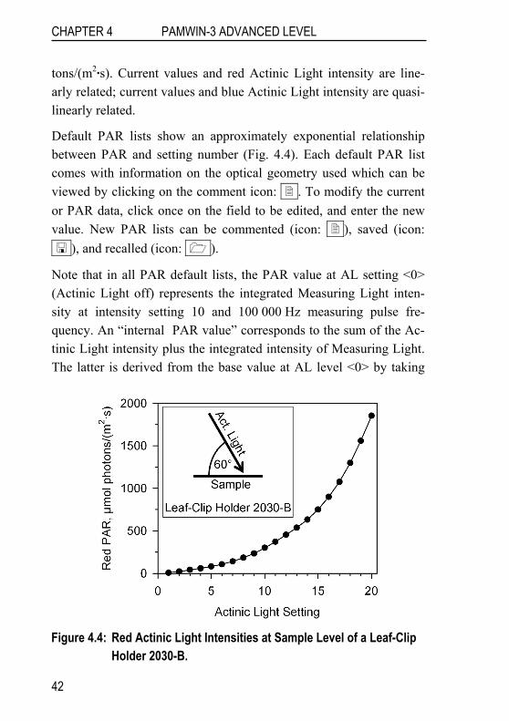
Default PAR lists show an approximately exponential relationship between PAR and setting number (Fig. 4.4). Each default PAR list comes with information on the optical geometry used which can be viewed by clicking on the comment icon: . To modify the current or PAR data, click once on the field to be edited, and enter the new value. New PAR lists can be commented (icon: ), saved (icon: ), and recalled (icon: ).
Note that in all PAR default lists, the PAR value at AL setting <0> (Actinic Light off) represents the integrated Measuring Light inten-sity at intensity setting 10 and 100 000 Hz measuring pulse fre-quency. An “internal PAR value” corresponds to the sum of the Ac-tinic Light intensity plus the integrated intensity of Measuring Light. The latter is derived from the base value at AL level <0> by taking
Figure 4.4: Red Actinic Light Intensities at Sample Level of a Leaf-Clip
Holder 2030-B.
42

PAMWIN-3 ADVANCED LEVEL CHAPTER 4
into account the frequency and intensity setting of the Measuring Light.
During setup of PamWin_3, the <default_60.par> file is automati-cally placed in the <C:\PamWin-3\Data_2500> directory together with additional PAR lists as specified in Table 4.1. The <de-fault_60.par> data are automatically loaded during the first start of the PamWin-3 software. The <default_60.par> list corresponds to the situation at sample level of a 2030-B Leaf-Clip Holder with the fiber optics fully inserted in the 60° port.
When the file <default_60.par> is not present in the <C:\PamWin-3\Data_2500> directory, factory values are used. Thereafter, at pro-gram start the most recently used PAR list is loaded.
Mode
In the <Mode> menu, the <VIEW> command switches to off-line operation: clicking on <MEASURE> reverses the latter action. The <VIEW> and <MEASURE> commands are equivalent to the VIEW-mode key in the <General Settings> Window (Fig. 4.3) and the MEASURE-mode key which is available in the off-line mode.
Table 4.1: Default Red and Blue PAR Lists: Intensities at Sample Level
File Name Sample Holder Optical Geometry*
default_60.par Leaf-Clip Holder 2030-B Distance Clip 2010-A Arabidopsis Leaf Clip 2060-B
60° 60°, 2 mm distance ring 60°, 6 mm distance ring
default_90.par Leaf-Clip Holder 2030-B 90°, 4 mm distance ring default_90_2060.par Arabidopsis Leaf Clip 2060-B 90°, 2 mm distance ring default_DLC.par Dark-Leaf-Clip DLC-8 90°
default_KS.par KS-2500 Suspension Cuvette 90° and 4 mm
*Detailed descriptions: see <Comment Files> attached to each PAR list.
43
CHAPTER 4 PAMWIN-3 ADVANCED LEVEL
Service
The <Service> menu is required for firmware update (the software residing on instrument processors is denoted firmware). New firm-ware is provided by the Walz Company. To determine your firmware version, click on the menu item <Read Firmware Version>.
Note: to avoid interruption of communication during firmware up-date, a stable power supply is mandatory: power failure can lead to malfunction of the processors, which then need to be re-programmed at the Walz Company.
To start firmware update, click <Controller Service>. The PAM-2500 contains 2 consecutively programmable processors: RISC and TINY (a tiny RISC processor).
a) RISC
Sequentially click on Program RISC Read HexFile Download HexFile .Then, the actual process of programming is initiated by clicking on the Program RISC key (this process re-quires some time). Finally, terminate the procedure by a mouse click on OK in the <Program RISC> window, confirm with OK the in-formation on program restart, and once again click OK in the <PAM-2500 Controller Service> window.
Before proceeding, close and restart the PamWin-3 program!
b) TINY
Programming the TINY processor is similar to the procedure ex-plained for the RISC processor. Start by clicking on Program TINY . Subsequently, click Read HexFile Download HexFile Program RISC . Finalize TINY pro-gramming by an OK in the <Program RISC> window, the (program
44
PAMWIN-3 ADVANCED LEVEL CHAPTER 4
restart) information window, and the <PAM-2500 Controller Ser-vice> window. Close and restart the PamWin-3 program.
<Trigger out with SP> This function puts out a 5 Volts trigger pulse with each Saturation Pulse. See Section 4.3.1.7 for a description of the trigger pins at the AUX connector and configuration of the trigger pulse.
Help
In the Help menu, checking Tooltips activates the PamWin-3 tooltips function described earlier (Section 4.1). Clicking on Info displays information on the current PamWin-3 version.
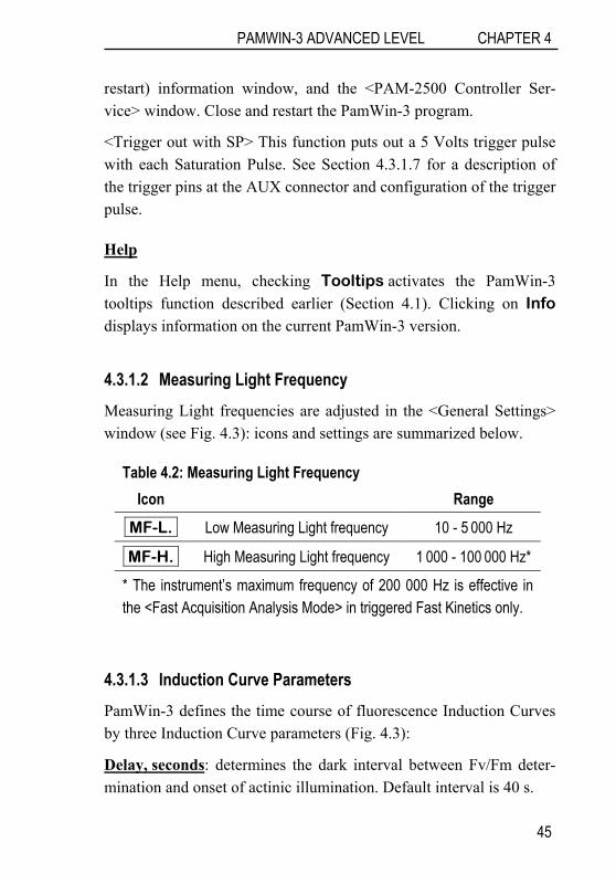
4.3.1.2 Measuring Light Frequency Measuring Light frequencies are adjusted in the <General Settings> window (see Fig. 4.3): icons and settings are summarized below.
Table 4.2: Measuring Light Frequency Icon Range
MF-L. Low Measuring Light frequency 10 - 5 000 Hz
MF-H. High Measuring Light frequency 1 000 - 100 000 Hz*
* The instrument’s maximum frequency of 200 000 Hz is effective in the <Fast Acquisition Analysis Mode> in triggered Fast Kinetics only.
4.3.1.3 Induction Curve Parameters PamWin-3 defines the time course of fluorescence Induction Curves by three Induction Curve parameters (Fig. 4.3):
Delay, seconds: determines the dark interval between Fv/Fm deter-mination and onset of actinic illumination. Default interval is 40 s.
45

CHAPTER 4 PAMWIN-3 ADVANCED LEVEL
Clock, seconds: defines the interval between Saturation Pulse analy-ses during actinic illumination.
Width, seconds: specifies the length of time of Actinic illumination.
All three time intervals are adjusted using upward and downward ar-row keys, or by double click on the interval number followed by manually entering the new time value. The AL-Width is automati-cally adjusted to equal a multiple of clock intervals plus 10 seconds. The extra 10 seconds are assigned to the initial and last Saturation Pulse applied during actinic illumination. Example: for a clock inter-val of 50 s, possible illumination times (<Width>) are 60 s, 110 s, 160 s …
4.3.1.4 Global Settings The PamWin-3 software allows to adjust numerous instrumental set-tings, so that an almost infinite number of setting combinations re-sults. Therefore, PamWin-3 offers the possibility to load a default set of standard settings and to save any particular set of settings which can be recalled later to carry out the same experiment with identical settings.
Four buttons manage the PAM-2500 <Settings> (see Global Settings in Fig. 4.3).
Default Installs default settings (File: <Walz2500.DEF>).
Open User Settings Loads previously stored settings except the Zoff which is set to zero when new <Settings> are loaded.
Save User Settings Saves the current setting to a file with for-mat <filename.DEF> except the Zoff.
46
PAMWIN-3 ADVANCED LEVEL CHAPTER 4
Write To Report Writes the settings to the current Report (see 4.4.3.1 for abbreviations used by a Report).
Other Commands
Zoff The <Zoff> (Zero Offset) serves to suppress a “background signal” which is not originating from the investigated sample. It is subtracted from all fluorescence signals. Background signals can arise from traces of scattered Measuring Light, which reaches the photo-detector. While this normally does not play a role in experi-ments with leaves, it may matter with suspensions at low chlorophyll content. In this case, the Zoff is determined with the cuvette contain-ing pure suspension medium by pressing Zoff . The <Zoff> can also be entered manually.
Exit PamWin shuts down PamWin-3
4.3.1.5 PAR Sensor Control Checking the <PAR Sensor Control> results in reading of data from an external PAR sensor. When the <PAR Sensor Control> is un-checked, PAR values are derived from the active internal light list. Internal Actinic Light arriving laterally at the entrance optics of the micro quantum sensor of the Leaf-Clip Holder 2030-B is not properly measured (Section 3.4.2.3). Therefore, when this sensor is connected, it should be disabled via <PAR Sensor Control> for applications in-volving actinic illumination by internal light sources (e.g. recording of Light Curves).
4.3.1.6 Fo, Fo’
Clicking the Fo icon (see Fig. 4.3) takes the present Ft fluorescence level as Fo level fluorescence that corresponds to the minimum fluo-
47
CHAPTER 4 PAMWIN-3 ADVANCED LEVEL
rescence of a dark-acclimated sample. Hence, an Fo measurement oc-curs without subsequent Fm determination, i.e., without exposing the sample to a saturating flash.
The C/Fo value indicates the relative contribution of a constant fluo-rescence fraction (which likely originates in PS I) to the measured Fo level fluorescence. The assessment of C/Fo requires that the Fo’ mode is activated and that non-photochemical fluorescence quench-ing decreases the Fo’ below the Fo level (see Section 5.3 for details).
Fo’ The Fo’ is the measured Fo’ level fluorescence. Checking the Fo’ box (Fig. 4.3) activates the Fo’ measuring mode. This means that a 5 seconds interval succeeds each Saturation Pulse during which the Actinic Light is switched off and <PS I light> is turned on. The PS I light quickly empties the PS II electron acceptor pool and, hence, opens the PS II reaction centers so that photochemical fluorescence quenching becomes maximal. The intensity of PS I light can be ad-justed in the <General Settings> window but the post-pulse time in-terval for far-red illumination is fixed.
˜Fo represents the calculated Fo’ level fluorescence. The ˜Fo’ is as-sessed from Fo, Fm, and Fm’ data according to Oxborough and Baker (1997; for details see Section 5.1.2).
4.3.1.7 Tab Bar Each active window of PamWin-3 appears as a tab in the Tab Bar, and clicking on a tab moves the respective window to the foreground.
4.3.1.8 Pulses, Short Term Illumination The advanced level offers additional ways of sample illuminations but also the possibility to apply a trigger signal to control an external device (Fig. 4.3).
48
PAMWIN-3 ADVANCED LEVEL CHAPTER 4
34
5
6
1
2
7
8
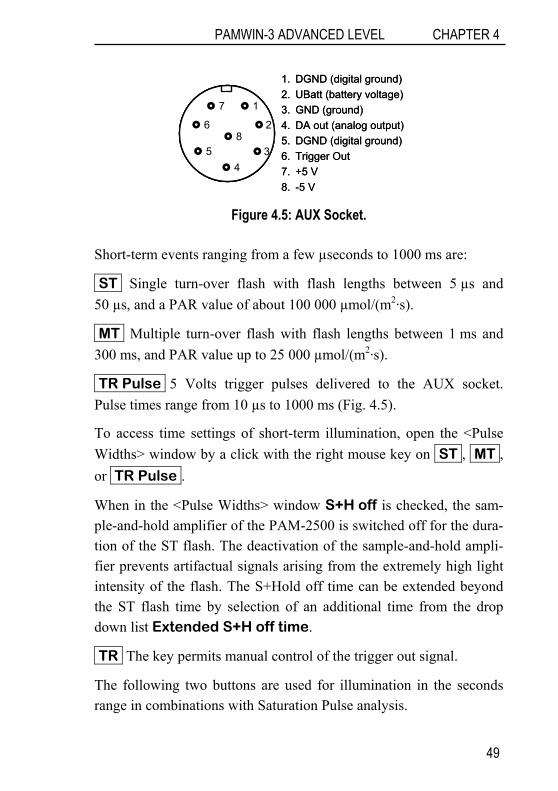
1. DGND (digital ground)2. UBatt (battery voltage)3. GND (ground)4. DA out (analog output)5. DGND (digital ground)6. Trigger Out7. +5 V8. -5 V
34
5
6
1
2
7
83
45
6
1
2
7
8
1. DGND (digital ground)2. UBatt (battery voltage)3. GND (ground)4. DA out (analog output)5. DGND (digital ground)6. Trigger Out7. +5 V8. -5 V
Figure 4.5: AUX Socket.
Short-term events ranging from a few µseconds to 1000 ms are:
ST Single turn-over flash with flash lengths between 5 µs and 50 µs, and a PAR value of about 100 000 µmol/(m2·s).
MT Multiple turn-over flash with flash lengths between 1 ms and 300 ms, and PAR value up to 25 000 µmol/(m2·s).
TR Pulse 5 Volts trigger pulses delivered to the AUX socket. Pulse times range from 10 µs to 1000 ms (Fig. 4.5).
To access time settings of short-term illumination, open the <Pulse Widths> window by a click with the right mouse key on ST , MT , or TR Pulse .
When in the <Pulse Widths> window S+H off is checked, the sam-ple-and-hold amplifier of the PAM-2500 is switched off for the dura-tion of the ST flash. The deactivation of the sample-and-hold ampli-fier prevents artifactual signals arising from the extremely high light intensity of the flash. The S+Hold off time can be extended beyond the ST flash time by selection of an additional time from the drop down list Extended S+H off time.
TR The key permits manual control of the trigger out signal.
The following two buttons are used for illumination in the seconds range in combinations with Saturation Pulse analysis.
49

CHAPTER 4 PAMWIN-3 ADVANCED LEVEL
AL + Y The command illuminates the sample with Actinic Light as defined in <General Settings> and thereafter carries out a Saturation Pulse analysis. This command is available for Actinic Light widths of 3 s or longer. With appropriate choice of AL Intensity and Width, AL+Y measurements can provide essential information on the photo-synthetic performance of a sample and is well suited for the screening of deficiencies.
FR + Y This command works similarly as the <AL + Y> command except for the Actinic Light being replaced by PS I light.
4.3.1.9 Mode The mode area in the <General Settings> window (Fig. 4.3) represent a hub leading to different program levels, that is, the three PamWin-3 measuring modes (Field Screen, Advanced SP-Analysis and Ad-vanced Fast Acquisition) and the PamWin-3 <View> mode for off-line data evaluation. In the Fast Acquisition mode, emphasis is on the recording of kinetic changes. While the same multiple turnover satu-rating light pulses (MT) can be applied as in the SP-Analysis mode, there is no automatic determination of fluorescence parameters. An exception is the <Fo, Fm> determination, with calculation of Fv/Fm.
4.3.1.10 Clock Event In total, 6 different events can be repetitively triggered by the clock function. All events are defined under <General Settings> except for the light curve which is defined on the <Light Curve> window. Theoretically, the interval time between events ranges from 3 to 900 seconds. Practically, the minimum interval needs to be longer than the event time plus some extra time to allow for data processing. The clock-triggered events are:
50
PAMWIN-3 ADVANCED LEVEL CHAPTER 4
SAT-Pulse: Saturation Pulse with quenching analysis.
AL: illumination with Actinic Light for a time period de-fined under General Settings/Act.Light/Width.
AL + Y: illumination with Actinic Light for a time period de-fined under General Settings/Act.Light/Width, fol-lowed by a Saturation Pulse with quenching analysis.
FR + Y: illumination with PS I light for a time period defined under General Settings/PS I Light/Width, followed by a Saturation Pulse with quenching analysis.
Light Curve: Light Curve defined in the Light Curve Edit window.
Slow Induc. Fluorescence Induction curve (Kautsky-effect), as defined under General Settings/Slow Induction.
4.3.1.11 New Record In the SP-Analysis Mode, data are grouped as <Records>. A new <Record> is started by clicking on the New Record button which becomes activated at the first <Fo, Fm> determination after program start. Starting a new <Record> does not interrupt continuous re-cording in the <Slow Kinetics> graph.
Usually, a <Record> starts with an <Fo, Fm> determination using a dark-adapted sample. The Fo and Fm level fluorescence enters the calculations of many fluorescence ratio parameters (see Chapter 5). It is therefore important to carry out proper <Fo, Fm> determinations and to correctly organize the recording of Saturation Pulse data (i.e. assigning one <Record> to each sample).
51

CHAPTER 4 PAMWIN-3 ADVANCED LEVEL
4.4 SP-Analysis Mode
4.4.1 Slow Kinetics Window The primary function of the <Slow Kinetics> window is real-time display of fluorescence kinetics, Ft, and of fluorescence ratio parame-ters derived from Saturation Pulse analysis. The new graphical ele-ments of the <Slow Kinetics> window are displayed in Figure 4.6. The figure does not show the elements already introduced in the pre-vious section (<General Settings>).
The <Menu Bar> of the <Slow Kinetics> and <General Settings> windows are similar except the <File> menu which contains as addi-
Figure 4.6: Slow Kinetics Window.
52
PAMWIN-3 ADVANCED LEVEL CHAPTER 4
tional commands <Print Graph> and <Save as pws-file>. Execution of the latter command saves the current Ft fluorescence trace in the “PamWin Slow Kinetic” format (*.pws). In the <View> mode, the Ft file can be opened and converted into text format to be imported by other programs.
4.4.1.1 Graph Icons The three graph icons outlined in Fig. 4.6 control display of the graph grid (left icon), automatic scaling of both graph axes (central icon), and printing of the current graph (right icon).
4.4.1.2 Graph Y, X The left and right numerical display fields (Fig. 4.6) indicate the x (time in s) and y (relative units) coordinates, respectively, of the cur-sor position in the graphics field.
4.4.1.3 Save Ft The disk icon ( , see Fig. 4.6) is identical to the <Save as pws-file> command in the <File> menu. The document icon ( ) opens the comment file associated with the most recently saved Ft fluores-cence trace.
4.4.1.4 Display Control Display of the various fluorescence parameters are controlled by checkboxes (see <Display Control>, Fig. 4.6). The data points and background colors of the corresponding checkbox labels have identi-cal colors.
53

CHAPTER 4 PAMWIN-3 ADVANCED LEVEL
4.4.1.5 X-Axis Scaling/Zoom In
Clicking on the arrow directing to the left (◄, see Fig. 4.6) increases the total x axis time range by a factor 2, while the total x axis time range is divided by 2 when the arrow directing to the right (►) is clicked.
In addition to the x-axis scaling buttons, both, x- and y-scaling can be modified to magnify a particular part of the graph: to “Zoom in”, click with the left mouse button on the left upper border of the target area, move the mouse with the left button pressed down to the right lower border of target area, and release the mouse button (see Fig. 4.6). A right mouse click anywhere on the graph field restores the original display.
The currently displayed graph can be moved vertically by pressing <Shift> key and gripping the graph with the left mouse button. With the <Ctrl> button depressed, the mouse moves the graph horizontally.
4.4.1.6 Slow Kinetics Control The drop-down menu in the <Slow Kinetics Control> area (Fig. 4.6) allows to choose between a manually controlled recordings (Manual), automated recordings of dark-light fluorescence induction curves (Ind.Curv.) or dark-light induction curves followed by an extended dark recovery time, during which the relaxation of non-photochemical quenching is monitored (Ind.+Rec.).
The Start and Stop buttons in the < Slow Kinetics Control> area start and end a <Record>. Several <Records> can be stored in one <Report>.
Recordings of Ind.Curv. And Int.+Rec. are always initiated by automated <Fo, Fm> measurements and the Fm serves for scaling the Ft signal between 0 and 1 (ordinate scale corresponding to Ft/Fm).
54
PAMWIN-3 ADVANCED LEVEL CHAPTER 4
The same scale also applies to the fluorescence ratio parameters, ex-cept for NPQ, which can assume values above 1. Therefore, NPQ/4 values are plotted.
Manual recordings can be carried out without <Fo, Fm> measure-ments. In this case, the Ft signal is recorded using the original voltage scale. For full quenching analysis, however, an <Fo, Fm> determina-tion is required (cf. Chapter 5).
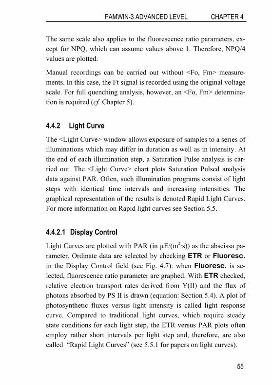
4.4.2 Light Curve The <Light Curve> window allows exposure of samples to a series of illuminations which may differ in duration as well as in intensity. At the end of each illumination step, a Saturation Pulse analysis is car-ried out. The <Light Curve> chart plots Saturation Pulsed analysis data against PAR. Often, such illumination programs consist of light steps with identical time intervals and increasing intensities. The graphical representation of the results is denoted Rapid Light Curves. For more information on Rapid light curves see Section 5.5.
4.4.2.1 Display Control Light Curves are plotted with PAR (in µE/(m2·s)) as the abscissa pa-rameter. Ordinate data are selected by checking ETR or Fluoresc. in the Display Control field (see Fig. 4.7): when Fluoresc. is se-lected, fluorescence ratio parameter are graphed. With ETR checked, relative electron transport rates derived from Y(II) and the flux of photons absorbed by PS II is drawn (equation: Section 5.4). A plot of photosynthetic fluxes versus light intensity is called light response curve. Compared to traditional light curves, which require steady state conditions for each light step, the ETR versus PAR plots often employ rather short intervals per light step and, therefore, are also called “Rapid Light Curves” (see 5.5.1 for papers on light curves).
55
CHAPTER 4 PAMWIN-3 ADVANCED LEVEL
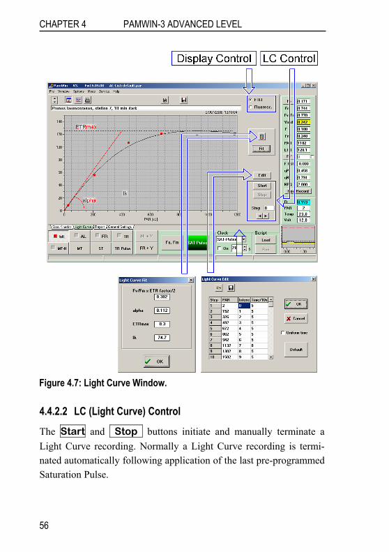
Figure 4.7: Light Curve Window.
4.4.2.2 LC (Light Curve) Control
The Start and Stop buttons initiate and manually terminate a Light Curve recording. Normally a Light Curve recording is termi-nated automatically following application of the last pre-programmed Saturation Pulse.
56

PAMWIN-3 ADVANCED LEVEL CHAPTER 4
4.4.2.3 Light Curve Edit Programming of the Light Curve parameters are done in the <Light Curve Edit> window (see Fig. 4.7). Up to 20 illumination steps can be programmed. A particular Light Curve illumination program can be saved as Light Curve Program and loaded again at any later time using the icons on the top of the <Light Curve Edit> window. The default light curve file is denoted <default.lcp>.
Programmable parameters are the PAM-2500 Actinic Light intensity setting (1 to 20 in Intens. column) and the time intervals of a light intensity step (in 10 seconds intervals, Time/10s). To change set-tings, click in the target field once and type in the new number. The change becomes effective upon the next click. To set the same illu-mination interval for all steps, check <Uniform time>, before enter-ing the desired time and terminating with another click. A zero in the Time/10s column ends exposure (e.g., when “0 seconds” is attrib-uted to step 6, only steps 1 to 5 will be executed.) When the 0 is en-tered, <Uniform time> should be disabled.
The light intensities used as x-values correspond to those of the se-lected internal PAR list. It is not recommended to measure the PAR online (see Section 3.4.2.3). If the Leaf-Clip 2030-B is connected, the PAR sensor should be disabled under General settings.
4.4.2.4 Light Curve Fit The equation derived by Eilers and Peeters (Ecological Modelling 42 (1988) 199-215) is used to describe rapid light curves. From the re-sults of curve fitting, three cardinal parameters are calculated (see Fig. 4.7):
alpha: The initial slope of the rapid light curve which is related to the maximal quantum yield of PS II electron transport under light limited conditions (unit: electron/photon).
57

CHAPTER 4 PAMWIN-3 ADVANCED LEVEL
ETRmax: The maximal relative electron transport rate reached dur-ing Light Curve recording (unit: µmol e-/(m2·s)), which reflects the light saturated capacity of the sample.
Ik: The light intensity at which the alpha and ETRmax lines intersect (unit: µmol photons/(m2·s)), which may be considered a proxy for the PAR where saturation sets in.
In the Light Curve Fit window, besides the three cardinal parameters obtained from the fitting procedure, also the Fv/Fm x ETR factor/2 is displayed. This is meant to remind that Fv/Fm corresponds to the maximal quantum yield of charge separation at PS II reaction centers, from which the parameter alpha can be predicted, when the ETR fac-tor (normally 0.84) and the fraction of quanta distributed to PS II (normally 0.5) are considered. The Fv/Fm x ETR factor/2 tends to be somewhat larger than alpha, due to some decrease of Y(II) at low light intensities.
4.4.3 Report Generally, a Report file consists of a list of data measured by Satura-tion Pulse analysis. The data are organized by date/time and columns of the various measured parameters. The user may add comments with additional information on the particular measurements. A Report file can contain several Records, each of which normally represent a series of Saturation Pulse analyses with the same sample.
4.4.3.1 Report Data Management A Report file can contain up to 1600 Saturation Pulse analyses. The percentage of file space used is indicated numerically and graphically (see <Report Data Management> in Fig. 4.8). The window area <Re-port Data Management> also provides icons to access the current
58
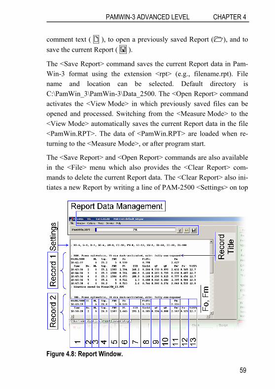
PAMWIN-3 ADVANCED LEVEL CHAPTER 4
comment text ( ), to open a previously saved Report ( ), and to save the current Report ( ).
The <Save Report> command saves the current Report data in Pam-Win-3 format using the extension <rpt> (e.g., filename.rpt). File name and location can be selected. Default directory is C:\PamWin_3\PamWin-3\Data_2500. The <Open Report> command activates the <View Mode> in which previously saved files can be opened and processed. Switching from the <Measure Mode> to the <View Mode> automatically saves the current Report data in the file <PamWin.RPT>. The data of <PamWin.RPT> are loaded when re-turning to the <Measure Mode>, or after program start.
The <Save Report> and <Open Report> commands are also available in the <File> menu which also provides the <Clear Report> com-mands to delete the current Report data. The <Clear Report> also ini-tiates a new Report by writing a line of PAM-2500 <Settings> on top
Figure 4.8: Report Window.
59
CHAPTER 4 PAMWIN-3 ADVANCED LEVEL
of the new line: the line of PAM-2500 <Settings> includes 16 pa-rameters (see Table 4.3). Similarly, the <Write to Report> command on the <General Settings> window creates PAM-2500 <Settings> line.
Table 4.3: Report of Instrument Settings Abbreviation Parameter AI Actinic Light Intensity AW Actinic Light Width BI Blue Light Intensity BW Blue Light Width D Damping FI Far-red Light Intensity FW Far-red Light Width G Gain H High Measuring Frequency ID Slow Induction Delay II Slow Induction Clock IS Slow Induction Actinic Light Width L Low Measuring Frequency MI Measuring Light Intensity SI Saturating Pulse Intensity SW Saturating Pulse Width
4.4.3.2 Record Header and Last Line First Line: Record Title The first line of a Record contains the Record title. A Record title is written automatically, if entered in the text field above the graphics chart in the <Slow Kinetics> or <Light Curve> window. It can also be written manually. In this case, just like with any other text com-ment line, the text must begin with a semicolon (;) for distinction from data lines.
60
PAMWIN-3 ADVANCED LEVEL CHAPTER 4
Second and Third Line: Fo, Fm The second and third Record lines contain data related to an <Fo, Fm> determination, which normally should be carried out at start of a new Record. The abbreviations <IC> and <IC+> in the second line indicate that the measuring programs <Induction Curve> and <Induction Curve and Recovery>, respectively, have been started.
Notes: (1) when <Fo, Fm> determination is not the first Saturation Pulse analysis of a Record, and when the graphics text field is left blank, lines 1 to 3 are reduced to the date of the experiment, (2) an <Fo, Fm> determination does not start a new Record, (3) a <Fo, Fm> determination during a Record is not indicated in the Record, but the Fo and Fm values are used for calculations of fluorescence ratio pa-rameters.
Last Line: Saving of Slow Kinetics file
If the Slow Kinetics measured during the Record was saved, the cor-responding file name is documented in the last line.
4.4.3.3 Record Columns In the measuring mode, a Record chart contains 12 columns. More data are available in the <View> mode. The subsequent comments on Report columns use the column numbering depicted in Fig. 4.8.
1 Date and time. 2 Sequential numbering of Saturation Pulses. The number <1> is
omitted if the first Saturation Pulse was applied to determine <Fo, Fm>.
3 Setting of Measuring Light intensity 4 Temperature (°C) 5 Actinic light intensity (PAR, µmol photons/(m2·s)).Light inten-
sity (PAR, µmol photons/(m2·s).
61

CHAPTER 4 PAMWIN-3 ADVANCED LEVEL
6 Fo (header lines) and F (subsequent data lines) in Volts. 7 Electron transport rate (ETR, µmol electrons/(m2·s)) 8 Maximum (header lines) and effective photochemical quantum
yield (subsequent data lines) of PS II 9 Coefficient of photochemical fluorescence quenching (qP). Set
to 1.000 in the absence of appropriate Fo and Fm data. 10 Coefficient of non-photochemical fluorescence quenching. Set
to 0.000 in the absence of appropriate Fo and Fm data. 11 Fm (header lines) and Fm’ (subsequent data lines) in Volts. 12 Fo’ data as determined with the help of far-red illumination. If
the Fo’-mode is not selected, column 12 stays blank. 13 Battery voltage (Volts).
4.5 Fast Acquisition Mode The <Fast Acquisition Mode> of PamWin-3 allows to study fluores-cence kinetics in the sub-msec to sec range using a maximum time resolution of 10 µs. This mode is specialized for well-defined trig-gered illumination by red, blue or far-red light. The measured fluo-rescence changes can be averaged and in this way an excellent signal-to-noise ratio can be obtained at high time resolution even with weakly fluorescent samples. Except for calculation of Fv/Fm, no SP analysis is carried out. According to the different mode of analysis, three windows present in the SP-analysis mode (<Slow Kinetics>, <Light Curve>, and <Report>) are replaced by the <Fast Kinetics> and <Fast Settings> windows. The new features of these windows will be introduced next.
4.5.1 Fast Settings The <Fast Settings> window represents the user surface to program timing and light conditions of fast kinetics recordings. In this win-dow, the various tools required to design a particular fast kinetics
62

PAMWIN-3 ADVANCED LEVEL CHAPTER 4
trigger program are grouped in different window areas according to their functionality (Fig. 4.9).
4.5.1.1 Basic Settings Rate/Points The sampling rate corresponds to the time interval be-tween two consecutive ML pulses. The rate thus determines time resolution. The total time interval of a <Fast Kinetics> recording is determined by the product of the sampling rate and the number of points. A trigger signal cannot be programmed at times exceeding
Figure 4.9: Fast Settings Window.
63

CHAPTER 4 PAMWIN-3 ADVANCED LEVEL
32 000 points, while the overall <Fast Kinetics> may comprise up to 128 000 points. For example, a <Fast Kinetics> can be composed of an initial fluorescence rise, induced by triggered illumination, which is followed by a fluorescence decay curve.
Target Averages The “Target Averages” correspond to the num-ber of Fast Kinetics recordings that will be averaged, when Averag-ing is enabled via the <Averaging> checkbox in the <Fast Kinetics> window. Consecutive recordings can be either triggered manually (Fast Kin. button / Start button) or via the Clock.
4.5.1.2 Menu Bar The composition the <Menu Bar> in the <Fast Kinetics> and the <SP-Analysis> mode is mostly identical (Section 4.3.1.1) except the items listed in the <Window> menu which correspond to the win-dows available in the current mode.
4.5.1.3 Trigger Settings ( I ) and ( II ) To configure trigger signals, 6 different tool icons are provided (see Figs. 4.9 and 4.10). The 3 left-most icons in Fig. 4.10 represent commands which affect the entire trigger signal but the three icons on the right hand side configure signal changes of various lengths which is shorter than the total trigger interval.
Figure 4.10: Trigger Tool Icons.
64
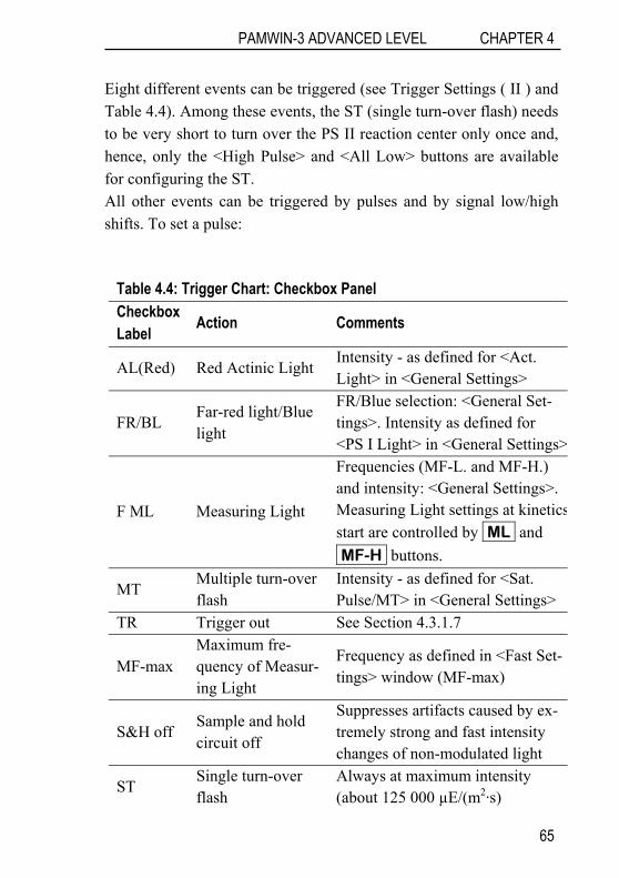
PAMWIN-3 ADVANCED LEVEL CHAPTER 4
Eight different events can be triggered (see Trigger Settings ( II ) and Table 4.4). Among these events, the ST (single turn-over flash) needs to be very short to turn over the PS II reaction center only once and, hence, only the <High Pulse> and <All Low> buttons are available for configuring the ST. All other events can be triggered by pulses and by signal low/high shifts. To set a pulse:
Table 4.4: Trigger Chart: Checkbox Panel Checkbox Label Action Comments
AL(Red) Red Actinic Light Intensity - as defined for <Act. Light> in <General Settings>
FR/BL Far-red light/Blue light
FR/Blue selection: <General Set-tings>. Intensity as defined for <PS I Light> in <General Settings>
F ML Measuring Light
Frequencies (MF-L. and MF-H.) and intensity: <General Settings>. Measuring Light settings at kineticsstart are controlled by ML and MF-H buttons.
MT Multiple turn-over flash
Intensity - as defined for <Sat. Pulse/MT> in <General Settings>
TR Trigger out See Section 4.3.1.7
MF-max Maximum fre-quency of Measur-ing Light
Frequency as defined in <Fast Set-tings> window (MF-max)
S&H off Sample and hold circuit off
Suppresses artifacts caused by ex-tremely strong and fast intensity changes of non-modulated light
ST Single turn-over flash
Always at maximum intensity (about 125 000 µE/(m2·s)
65
CHAPTER 4 PAMWIN-3 ADVANCED LEVEL
a) Select an event by clicking on its checkbox label (Fig. 4.9. Trigger Setting ( II )). The event is selected when its label is typed white on blue background.
b) Activate event by clicking the box associated with the label.
c) Click on <High Pulse> icon.
d) Select time interval in drop-down menu. Note that the <ST Width> menu applies for ST only, but pulse lengths of the other events must be selected in the <Pulse Width> menu. Also, the minimum pulse width depends on the sampling rate selected (Fig. 4.9. Basic Settings).
e) Click in the field below <Trig on, µs> (see Fig. 4.9. Trigger Setting ( II )) and type in the time point of pulse start in µs. Hitting the <Enter> key results in the digital display of the pulse end time in the neighboring data field (calculated with the interval selected above), and in the graphical display in the <Trigger Graph>.
Repeating step e) places an additional pulse on the same trigger line. For the same event, pulse intervals may vary: simply visit step d) be-fore proceeding to e). To move to the next event, simple select and activate the event (steps a) and b), respectively).
Longer-term triggering is achieved by using the <Toggle Low/High> tool (Fig. 4.10). Basically, the procedure is identical to the setting of trigger pulses but in step c) the <Toggle Low/High> icon must be se-lected and, in step e), the setting of the <Trig on, µs> time point does not automatically results in an entry in the <Trig off, µs> field. Con-sequently, the trigger signal can be
- switched only from low to high (no entry in the <Trig off, µs> field)
66

PAMWIN-3 ADVANCED LEVEL CHAPTER 4
- switched only from high to low (no entry in the <Trig off, µs> field followed by the <Invert All> command. Fig. 4.10.), or
- switched from low to high and then back at the time points en-tered in the <Trig on, µs> and <Trig off, µs> fields, respectively.
Table 4.5: Fast Settings - Trigger Program Tools*
Action ActiveIcon Key Combination Parameters
M a i n T r i g g e r C h a r t High pulse*,**
<Shift> + <right mouse key> All
Low pulse*,**
<Shift> + <right mouse key> All
Switch to high**
<Shift> + <left mouse key> All but ST
Switch to low**
<Shift> + <right mouse key> All but ST
All low
All
All high
All but ST
Invert levels
First, select event to be triggered
(click on checkbox label) All
P r e t r i g g e r C h a r t Toggle between always high and always low
<right mouse key> All but ST
* For all events, <Pulse Width> applies except the ST interval which is determined by <ST Width>. Time points in µseconds of trigger on and off events are numerically displayed (see Fig. 4.9, Trigger Settings ( II ) ).
** Trigger setting via these shortcuts does not require selection of a trigger event in the checkbox panel.
67

CHAPTER 4 PAMWIN-3 ADVANCED LEVEL
Additionally, trigger pattern can be created by directly manipulating the <Trigger Chart> using the mouse pointer as outlined in Table 4.5. The graphical editing of trigger lines is facilitated by the numerical displays of the mouse cursor position (numerical displays below <Trigger Tool Icons>).
For accurate setting of time points, the x axis can be enlarged as out-lined in Table 4.6 which also comments on how to shift the x axis af-ter enlargement.
Trigger files can be saved and recalled using the appropriate icons in the <Trigger Settings ( I )> field: and , respectively. Click-ing the Default button in <Trigger Settings ( I )> opens the <Poly300ms.FTM> which is one of the predefined trigger files of PamWin-3.
When Enable Pretrigger is checked (Trigger Settings ( II ), Fig. 4.9), a display field appears below the checkbox, which is associated with a drop down list of pretrigger time intervals. Also, a small chart,
Table 4.6: Fast Settings - Chart Manipulation Action Key Combination
Enlarge x-axis scale
Click with <left mouse key> at lower x limit, while keeping the mouse key de-pressed move cursor to the upper x limit, release key.
Switch between enlarge x-axis and shift x-axis
Single <right mouse key> on trigger chart
Shift x-axis Click on chart with <left mouse key>, hold mouse key down and move cursor horizon-tally
Full x-axis scale <Auto button>
68

PAMWIN-3 ADVANCED LEVEL CHAPTER 4
entitled <Pre>, left of the <Trigger Graph> becomes apparent. In the <Pre> chart, a trigger signal can be toggled between low and high by left-clicking on trigger line. A pretriggered event is active for the pre-trigger time interval selected. The pretrigger interval is immediately followed by the fast kinetics. Note that, different to the main trigger pattern, the pretrigger settings are not set <All Low> by the Clear All button.
Zero Time Shift (Trigger Settings ( II ), Fig. 4.9) right-shifts the zero point of the time axis so that recording of a fast kinetics starts at negative time values but triggered action can be initiated at zero or positive time points. Zero time shift is advantageous when fluores-cence data are plotted against a logarithmic time scale. To adjust the zero time shift, double-click on the number displayed below the phrase <Zero Time Shift> and enter the new time value.
4.5.1.4 Light & Pulses In the <fast acquisition> mode, two buttons are available which first start an illumination with Actinic or far-red light and then initiate the execution of a fast kinetics (Fig. 4.9):
The AL + F.K. command starts an Actinic illumination and then executes the current trigger pattern.
The FR + F.K. is similar to the previous command except that far-red illumination is given instead of Actinic Light.
Note: the illumination regimes of AL + F.K. / FR + F.K. differ from the pretrigger illumination (see previous Section) because the Actinic/far-red light stays on during the fast kinetics. The time inter-val for Actinic/far-red light must be defined in <General Settings>; the fast kinetics will be performed 2 seconds before the time interval ends.
69
CHAPTER 4 PAMWIN-3 ADVANCED LEVEL
4.5.1.5 Start Fast Kinetics
Fo, Fm Clicking the <Fo, Fm> button starts determinations of Fo and Fm values, calculation of the Fv/Fm and entry of the data in the current Report as described in Section 4.2.1.3.
_Start_ The command starts immediate execution of the current trigger pattern.
Clock Three different events can be triggered by the <Clock> func-tion in the <Fast Kinetics> mode: fast kinetics, fast kinetics in the presence of illumination with Actinic Light, and fast kinetics in the presence of illumination with far-red light. The three events are equivalent to the commands <Start>, <AL + F.K.>, and <FR + F.K.> (see above). The clock interval can be set using the up and down ar-rows, but the interval can also be entered manually after double-click on the displayed time interval.
4.5.2 Fast Kinetics The data acquired in the <Fast Kinetics> mode are displayed in the <Fast Kinetics> window. Most options available for axis control in the <Slow Kinetics> Window (Section 4.4.1) also work with the <Fast Kinetics> window. The new features of the <Fast Kinetics> graphics display are:
- Control of y-axis scaling by up ( ▲ )/down ( ▼ ) arrows, and by Auto button (Fig. 4.11, Axis Control).
- Toggling option to switch between linear and logarithmic x-axis scaling (see Log checkbox Fig. 4.11).
- Keep Scale function to fix y-axis scaling when viewing a series of fast kinetics recorded at different y-axis scales (Fig. 4.11, y-axis scaling).
70
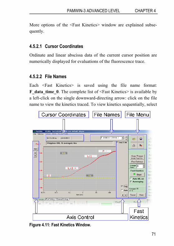
PAMWIN-3 ADVANCED LEVEL CHAPTER 4
More options of the <Fast Kinetics> window are explained subse-quently.
4.5.2.1 Cursor Coordinates Ordinate and linear abscissa data of the current cursor position are numerically displayed for evaluations of the fluorescence trace.
4.5.2.2 File Names Each <Fast Kinetics> is saved using the file name format: F_data_time_0. The complete list of <Fast Kinetics> is available by a left-click on the single downward-directing arrow: click on the file name to view the kinetics traced. To view kinetics sequentially, select
Figure 4.11: Fast Kinetics Window.
71

CHAPTER 4 PAMWIN-3 ADVANCED LEVEL
a file name in the list of <Fast Kinetics>, use the Up/Down arrow pair to the right of the file name display, or the up/down arrows on your keyboard, or the mouse wheel.
4.5.2.3 File Menu <Fast Kinetics> which are not saved will be lost at closure of Pam-Win-3. Kinetics can be saved as Pam Fast Kinetics files (*.pfk) using the floppy disk icon in the <File Menu> (see Fig. 4.11). Also, data can be exported (icon below floppy disk icon) in ASCII or Unicode formats which are importable by most spreadsheet and graphing pro-grams.
4.5.2.4 Fast Kinetics A number of elements to manage fast kinetics are pooled in the <Fast Kinetics> panel (see Fig. 4.11).
Copy Trigger from Fast Kin. Clicking this icon overwrites the current trigger pattern with the trigger pattern associated with the cur-rently displayed kinetics. The feature aids to reproduce kinetics.
Fast Settings The command switches to the <Fast Settings> win-dow.
Average Points The figure displays corresponds to the number of points averaged for graphical display. The “graphical averaging” does not affect the originals data.
Start The command starts immediate execution of the current trig-ger pattern.
Auto ML On If checked, the Measuring Light is switched at start of a <Fast Kinetics>.
72
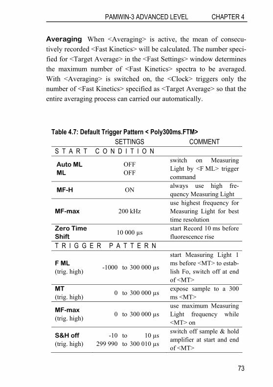
PAMWIN-3 ADVANCED LEVEL CHAPTER 4
Averaging When <Averaging> is active, the mean of consecu-tively recorded <Fast Kinetics> will be calculated. The number speci-fied for <Target Average> in the <Fast Settings> window determines the maximum number of <Fast Kinetics> spectra to be averaged. With <Averaging> is switched on, the <Clock> triggers only the number of <Fast Kinetics> specified as <Target Average> so that the entire averaging process can carried our automatically.
Table 4.7: Default Trigger Pattern < Poly300ms.FTM> SETTINGS COMMENT
S T A R T C O N D I T I O N
Auto ML ML
OFF OFF
switch on Measuring Light by <F ML> trigger command
MF-H ON always use high fre-quency Measuring Light
MF-max 200 kHz use highest frequency for Measuring Light for best time resolution
Zero Time Shift 10 000 µs start Record 10 ms before
fluorescence rise T R I G G E R P A T T E R N
F ML (trig. high) -1000 to 300 000 µs
start Measuring Light 1 ms before <MT> to estab-lish Fo, switch off at end of <MT>
MT (trig. high) 0 to 300 000 µs expose sample to a 300
ms <MT>
MF-max (trig. high) 0 to 300 000 µs
use maximum Measuring Light frequency while <MT> on
S&H off (trig. high)
-10 to 10 µs 299 990 to 300 010 µs
switch off sample & hold amplifier at start and end of <MT>
73

CHAPTER 4 PAMWIN-3 ADVANCED LEVEL
4.5.2.5 Polyphasic Fluorescence Rise Here, the default trigger pattern of PamWin-3 (<Poly300ms.FTM>) is used to demonstrate aspects of trigger design for <Fast Kinetics>. The <Poly300ms.FTM> trigger pattern is shown in Fig. 4.9, and a fluorescence curve elicited by this trigger pattern is shown in Fig. 4.11.
Details of the <Poly300ms.FTM> trigger pattern are summarized in Table 1. In short, the triggering results in a <Fast Kinetics> which establishes a baseline in the absence of Measuring Light at negative time values. Shortly before time “zero”, high frequency Measuring Light is switched on the establish the Fo level fluorescence. At time zero, a polyphasic fluorescence kinetics is initiated by a strong multi turn-over flash and, simultaneously, the time resolution of measure-ment is further increased by switching to maximum frequency of Measuring Light. Figure 4.11 also depicts Fo and Fm level fluores-cence which were established by an <Fo, Fm> determination prior to recording a <Fast Kinetics>.
Generally, to become experienced with PamWin-3 trigger manage-ment, it is recommended to start with one of the trigger files provided by the software and then modify the default settings.
4.6 View Mode The <View Mode> of PamWin-3 is dedicated to analyses of fluores-cence measurements. Three windows are available in the <View Mode>: the <Report>, <Slow Kinetics> and <Light Curve> win-dows. The operation of the latter two windows is as described previ-ously (Sections 4.4.1 and 4.4.2).
The <Report> window in the <View Mode> provides new tools for data management and navigation; the <Icon Bar>, the <Sidebar>, and a panel for data selection (Fig. 4.12).
74
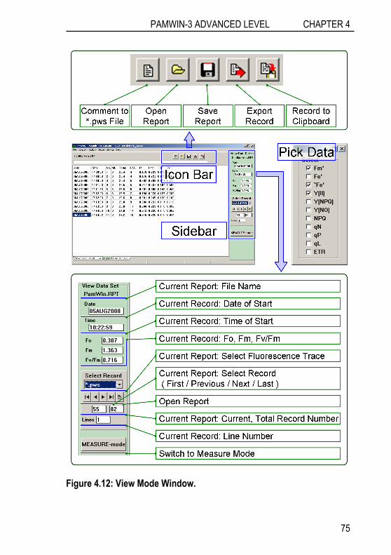
PAMWIN-3 ADVANCED LEVEL CHAPTER 4
Figure 4.12: View Mode Window.
75
CHAPTER 4 PAMWIN-3 ADVANCED LEVEL
4.6.1 Icon Bar The <Icon Bar> provides commands for opening Records, viewing comments and exporting data either as CSV data (comma separated values) or to clipboard (compare Fig. 4.12). The functions of the <Icon Bar> are also available in the <File> menu.
4.6.2 Sidebar The foremost function of the <Sidebar> (Fig. 4.12) is navigation within a <Report>. The various navigation functions for screening a <Report> are outlines in Fig. 4.12.
4.6.3 Pick Data The <Pick Data> panel gives access to all Saturation Pulse data and fluorescence ratio parameters except the C/Fo data. The selection of a parameter by ticking a checkbox results in the display of the respec-tive data in the <Record> data window: only the selected parameters are exported as CSV data or to the clipboard.
4.7 Script Files Script files are used for automatic execution of experimental proce-dures of various complexities. Carrying out experiments by Script files can be advantages when the same type of analysis needs to be repeated frequently or when complicated protocols must be exactly reproduced.
Generally, all manual operations and adjustments in the PamWin-3 software can also be carried out under the control of a Script file. In addition, Script files offer commands for time management, combina-tions of sub-programs and conditional commands.
76
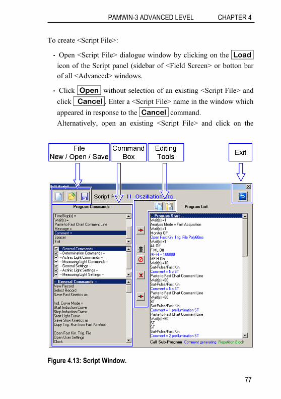
PAMWIN-3 ADVANCED LEVEL CHAPTER 4
To create <Script File>:
- Open <Script File> dialogue window by clicking on the Load icon of the Script panel (sidebar of <Field Screen> or botton bar of all <Advanced> windows.
- Click Open without selection of an existing <Script File> and click Cancel . Enter a <Script File> name in the window which appeared in response to the Cancel command. Alternatively, open an existing <Script File> and click on the
Figure 4.13: Script Window.
77

CHAPTER 4 PAMWIN-3 ADVANCED LEVEL
<New Script File> (Fig. 4.13: file icons).
The <Command Box> of the <Script File> window (Fig. 4.13) con-tains the available commands divided into 8 sections. In addition, the <Program Control Commands> are displayed on top of the <Com-mand Box>. The various functions of the latter commands are com-prehensibly elucidated in the <Help> attached to the <Command Box>.
All other command groups match the commands of manual instru-ment operation except the group <Condition Commands) which per-mit execution of an instructions depending on the state of a parameter like the fluorescence level or temperature.
A number of <Editing Tools> (Fig. 4.13) are provided to compose a Script file. Similar as for the <Command Box>, the <Help> associ-ated with the <Editing Tools> comprehensibly explains their func-tion.
78

DEFINITIONS & EQUATIONS CHAPTER 5
5 Definitions and Equations
5.1 Relative Fluorescence Yields Typically, five different types of fluorescence levels are acquired by Saturation Pulse analyses. Two of these levels need to be established with the dark-acclimated sample. The three remaining levels are re-peatedly measured during subsequent sample treatments (e.g., expo-sure to Actinic Light; see Fig. 7.1).
5.1.1 Measurements with dark-acclimated samples Fo Minimum fluorescence level excited by very low intensity of
Measuring Light to keep PS II reaction centers open.
Fm Maximum fluorescence level elicited by a strong light pulse which closes all PS II reaction centers.
5.1.2 Measurements with light-exposed (treated) samples Fo’ Minimum fluorescence level during a treatment. When the
measuring routine for Fo’ is active, the Fo’ level is deter-mined during a dark interval following the Saturation Pulse. In the dark interval, far-red light is applied to selectively drive PS I reaction centers and, thus, to quickly remove inter-system electrons and open PS II reaction centers (see Fig. 5.1, time point 75 s).
Alternatively, the Fo’ can be estimated according to Oxbor-ough and Baker (1997):
mF1
Fm1
Fo1
1oF
′+−
=′
79
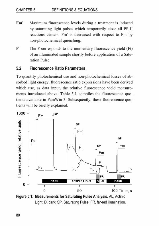
CHAPTER 5 DEFINITIONS & EQUATIONS
Fm’ Maximum fluorescence levels during a treatment is induced by saturating light pulses which temporarily close all PS II reactions centers. Fm' is decreased with respect to Fm by non-photochemical quenching.
F The F corresponds to the momentary fluorescence yield (Ft) of an illuminated sample shortly before application of a Satu-ration Pulse.
5.2 Fluorescence Ratio Parameters To quantify photochemical use and non-photochemical losses of ab-sorbed light energy, fluorescence ratio expressions have been derived which use, as data input, the relative fluorescence yield measure-ments introduced above. Table 5.1 compiles the fluorescence quo-tients available in PamWin-3. Subsequently, these fluorescence quo-tients will be briefly explained.
Figure 5.1: Measurements for Saturating Pulse Analysis. AL, Actinic Light; D, dark; SP, Saturating Pulse; FR, far-red illumination.
80

DEFINITIONS & EQUATIONS CHAPTER 5
Table 5.1: Fluorescence Ratio Parameters.
Source Equation
Maximum photochemical quantum yield of PS II (Kitajima and Butler, 1975)
FmFoFm
FmFv −
=
Effective photochemical quantum yield of PS II (Genty et al., 1989)
mFFmF)II(Y′−′
=
Coefficient of photochemical fluorescence quenching (Schreiber et al. 1986 as formulated by van Kooten and Snel, 1990)
oFmFFmFqP ′−′
−′=
Coefficient of photochemical fluorescence quenching assuming interconnected PS II an-tennae (Kramer et al. 2004)
FoFqq PL′
⋅=
Coefficient of non-photochemical fluorescence quenching (Schreiber et al. 1986 as formulated by van Kooten and Snel, 1990)
FoFmoFmF1qN −′−′
−=
Stern-Volmer type non-photochemical fluores-cence quenching (Bilger and Björkman, 1990) 1
mFFmNPQ −
′=
Quantum yield of non-regulated heat dissipa-tion and fluorescence emission: this quenching type does not require the presence of a trans-thylakoid ΔpH and zeaxanthin (Genty et al. 1996)*
FmF)NO(Y =
Quantum yield of light-induced (ΔpH- and ze-axanthin-dependent) non-photochemical fluo-rescence quenching (Genty et al. 1996)*
FmF
mFF)NPQ(Y −′
=
* Kramer et al. (2004) have derived more complex equations for Y(NO) and Y(NPQ). Klughammer and Schreiber (2008) have demonstrated that the equations by Kramer et al. (2004) can be transformed into the simple equa-tions of (Genty et al. 1996) which are used by PamWin-3 software.
81

CHAPTER 5 DEFINITIONS & EQUATIONS
Fv/Fm and Y(II) Maximum and effective photochemical quantum yield of PS II
Both fluorescence quotients estimate the fraction of absorbed quanta used for PS II photochemistry, (i.e., for stable charge separation in the PS II reaction center). For measurements of Fv/Fm, it is important that samples are acclimated to darkness or dim light so that all reac-tions centers are in the open state and non-photochemical dissipation of excitation energy is minimal. Requirements for dark acclimation can differ between plants: in extreme shade leaves, substantial clo-sure of PS II centers can occur already at PAR values of 0.1 μmol photons/(m2·s) but many sun leaves exhibit mostly open PS II centers even at 10-40 μmol μmol photons/(m2·s).
The Y(II) value estimates the photochemical use of excitation energy in the light. To derive from the Y(II) information on the overall state of photosynthesis, control of light conditions is required because a leaf may be severely damaged in Calvin cycle activity and still show a high value of Y(II) in weak light. Therefore, photosynthetic per-formance should be assessed during steady state illumination at a photon flux density which is somewhat below saturation in a control sample.
qP and qL Coefficients of photochemical fluorescence quenching.
Both parameters estimate the fraction of open PS II reaction centers. The qP is based on concept of separated PS II antennae (puddle model) but the qL assumes interconnected PS II antennae (lake model) which appears to be the more realistic situation in leaves (cf. Kramer et al., 2004). Determinations of qP an qL do not require fluo-rescence measurements with the dark-acclimated sample except when Fo’ is not measured but calculated according to Oxborough and Baker (1997) (see 5.1).
82

DEFINITIONS & EQUATIONS CHAPTER 5
qN and NPQ Parameters of non-photochemical quenching
Both parameters are associated with non-photochemical quenching of excitation energy by thylakoid lumen pH- and zeaxanthin-dependent processes. In contrast to Y(II), qP and qL, calculations of the qN and the NPQ parameters always require fluorescence measurements with the sample in the dark-acclimated and in the light-exposed state (see Table 5.1). Calculation of NPQ (or SVN; Gilmore and Yamamoto, 1991) corresponds to the Stern-Volmer equation for fluorescence quenching which predicts proportionality between fluorescence quenching (NPQ) and the concentration of fluorescence-quenching centers in the photosynthetic antennae (e.g. zeaxanthin).
Y(NO) and Y(NPQ) Yields of non-photochemical quenching
Genty et al. (1996) first presented expressions based on basic fluo-rescence parameters that describe the partitioning of absorbed excita-tion energy in PS II between three fundamental pathways, expressed in terms of the complementary quantum yields of
Y(NO) sum of non-regulated heat dissipation and fluorescence emission,
Y(NPQ) regulated thermal energy dissipation involving ∆pH- and zeaxanthin-dependent photoprotective mechanisms, and
Y(II) photochemical conversion
The yields of photochemical energy conversion and non-photochemical losses sum up to 1:
Y(II)+Y(NPQ)+Y(NO)=1
This concept of "complementary PS II quantum yields" is useful to analyze the partitioning of absorbed light energy in plants. For in-stance, under high light-conditions, a much higher Y(NPQ) than Y(NO) indicates that excess excitation energy is safely dissipated,
83
CHAPTER 5 DEFINITIONS & EQUATIONS
that is, photosynthetic energy fluxes are well-regulated. In variance, high values of Y(NO) would signify that excess excitation energy is moistly channeled off via basal quenching mechanisms and, hence, that energy fluxes are inadequately controlled.
5.3 Constant Fraction of Fo Fluorescence (C/Fo) A number of data suggest that PS I contributes significantly to room temperature fluorescence from leaves. Typical fractions of PS I con-tribution to total Fo fluorescence are 30 and 50% for C3 and NADP-ME C4 plants (e.g., maize), respectively (Genty et al. 1990, Pfündel 1998, Agati et al. 2000, Peterson et al. 2001, Franck et al. 2002).
Here, the assessment of <C/Fo> is based on the comparison of the Fo’ calculated according to Oxborough and Baker (1997) (see section 5.1.2) with the Fo’ determined during a post-Saturation Pulse illumi-nation with far-red light. Considering that PS I fluorescence contrib-utes a constant quantity, FPSI, to each fluorescence level, the Oxbor-ough-Baker equation can be reformulated:
PSIPSIPSIPSII
PSI
FmF1
FFm1
FFo1
1FoF
−′+
−−
−
+=′
In the latter equation, the FPSI is subtracted from the measured fluo-rescence levels Fo, Fm, and Fm’ so that the total fraction in the equa-tion above describes Fo’ originating in PS II. Clearly, the latter frac-tion plus the FPSI make up the total Fo’ signal. Compared to the origi-nal equation, the introduction of FPSI increases the calculated Fo’ be-cause the addition of FPSI overcompensates the effect of FPSI subtrac-tion. Consequently, when the FPSI is disregarded, theory underesti-mates the Fo’, and this is consistent with the observation that the cal-culated Fo’ is often lower the measured Fo’. Consequently, to assess
84
DEFINITIONS & EQUATIONS CHAPTER 5
the C/Fo, the PamWin-3 program iteratively varies the level of FPSI until the calculated Fo’ matches the measured Fo’.
In practice, determinations of C/Fo require that the Fo and Fm and
- Fully dark-acclimated material for accurate determination of Fo and Fm.
- Subsequent to Fo, Fm determinations, illumination with light in-tensity that induces substantial non-photochemical quenching but does not cause photoinhibition to measure Fo’ and Fm’.
5.4 Relative Electron Transfer Rate (ETR) Relative electron transfer rates are calculated according to:
ETR = PAR · ETR-Factor · PPS2/PPPS · Y(II).
The basic idea of the ETR equation is to multiply Y(II), the effective photochemical quantum yield of PS II, by an estimate for the photon flux density absorbed by PS II. The latter approximation uses three parameters which are explained below:
PAR Photosynthetically active radiation
Depending on settings, the PAR values of the active light list or measured data are used.
ETR-Factor Absorptance of photons by photosynthetic pigments
The ETR-Factor corresponds to the fraction of incident photons ab-sorbed by photosynthetic pigments. The default value for the ETR-Factor is 0.84 which is a reasonable match to the average absorptance in the visible range (400-700 nm) of many green leaves. Antho-cyanins, however, can reduce availability of blue photons for photo-synthesis (Pfündel et al. 2007) and, hence, lower the ETR-Factor.
85
CHAPTER 5 DEFINITIONS & EQUATIONS
PPS2/PPPS Photons absorbed by PS II relative to photons absorbed by photosynthetic pigments.
The default value for PPS2/PPPS is 0.5. This value is reasonable if one assumes only linear electron transport, that is, equal electron transfer rates though PS I and PS II, and comparable photochemical quantum yields of PS I and PS II under strongly light-limiting conditions.
The ETR may be compared to the rate of CO2-assimilation or of O2-evolution. For such comparison the following aspects are relevant:
- 4 e- must be transported for every CO2 assimilated or O2 evolved
- the value of ETR/4 is not necessarily identical to CO2-fixation rate or O2-evolution rate; discrepancies e. g. may arise from photorespiratory electron flow, nitrite reduction or electron cy-cling at PS II
- fluorescence information primarily originates from the topmost chloroplast layers, while gas exchange integrates over all layers; on the other hand, the topmost layers absorb most of the light and, hence, are also responsible for most of the gas exchange, unless photoinhibited.
The PAR can be measured at the same spot of the leaf where fluores-cence is measured, when the micro-quantum-sensor is moved into the beam. This is possible without substantial loss in signal amplitude. The properties of the micro-quantum-sensor are such that its response to spectral composition and incidence angle of the impinging light approximates that of the leaf
The combined information of ETR, PAR and Temperature provides profound insight into the photosynthetic performance of a plant. Plots of ETR versus PAR at different temperatures respond in a very sensi-tive manner to changes at all levels of the photosynthetic process (see next section).
86
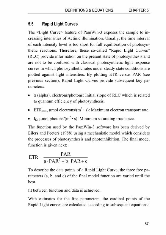
DEFINITIONS & EQUATIONS CHAPTER 5
5.5 Rapid Light Curves The <Light Curve> feature of PamWin-3 exposes the sample to in-creasing intensities of Actinic illumination. Usually, the time interval of each intensity level is too short for full equilibration of photosyn-thetic reactions. Therefore, these so-called “Rapid Light Curves” (RLC) provide information on the present state of photosynthesis and are not to be confused with classical photosynthetic light response curves in which photosynthetic rates under steady state conditions are plotted against light intensities. By plotting ETR versus PAR (see previous section), Rapid Light Curves provide subsequent key pa-rameters:
• α (alpha), electrons/photons: Initial slope of RLC which is related to quantum efficiency of photosynthesis.
• ETRmax, µmol electrons/(m2 · s): Maximum electron transport rate.
• IK, µmol photons/(m2 · s): Minimum saturating irradiance.
The function used by the PamWin-3 software has been derived by Eilers and Peeters (1988) using a mechanistic model which considers the processes of photosynthesis and photoinhibition. The final model function is given next:
cPARbPARaPARETR 2 +⋅+⋅
=
To describe the data points of a Rapid Light Curve, the three free pa-rameters (a, b, and c) of the final model function are varied until the best
fit between function and data is achieved.
With estimates for the free parameters, the cardinal points of the Rapid Light curves are calculated according to subsequent equations:
87

CHAPTER 5 DEFINITIONS & EQUATIONS
ca2bcI
ca2b1ETR
c1
K
max
⋅⋅+=
⋅⋅+=
=α
Figure 5.2 illustrates the behavior of the Eilers and Peeters model function for 3 theoretical cases which show identical values of α but, at high light intensities, different degrees of photoinhibition.
Figure 5.2: Three Exemplary Rapid Light Curves.
Curve Parameter a b c α ETRmax Ik
1 1·10-5 1·10-2 5 0.2 41 207 2 1·10-6 1·10-2 5 0.2 69 345 3 1·10-7 1·10-2 5 0.2 88 438
88
DEFINITIONS & EQUATIONS CHAPTER 5
5.5.1 Some Papers on Rapid Light Curves Fouqueray M, Mouget J-L, Morant-Manceau A, Tremblin AG (2007) Dynamics of short-term acclimation to UV radiation in marine dia-toms. J Photochem Photobiol B: Biology 89: 1–8
Jassby AD, Platt T (1976) Mathematical formulation of the relation-ship between photosynthesis and light for phytoplankton. Limnol Oceanogr 21: 540-547
Perkins RG, Mouget J-L, Lefebvre S, Lavaud J (2006) Light re-sponse curve methodology and possible implications in the applica-tion of chlorophyll fluorescence to benthic diatoms. Marine Biol 149: 703-712
Platt T, Gallegos CL, Harrison WG (1980) Photoinhibition of photo-synthesis in natural assemblages of marine phytoplankton. J Mar Res 38: 687-701
Ralph PJ, Gademann R (2005) Rapid light curves: A powerful tool to assess photosynthetic activity. Aquat Bot 82: 222-237
Rascher U, Liebig M, Lüttge U (2000) Evaluation of instant light-response curves of chlorophyll fluorescence parameters obtained with a portable chlorophyll fluorometer on site in the field. Plant Cell En-viron 23: 1397-1405
Schreiber U, Gademann R, Ralph PJ, Larkum AWD (1997) Assess-ment of photosynthetic performance of Prochloron in Lissoclinum patella in hospite by chlorophyll fluorescence measurements. Plant Cell Physiol 38: 945-951
Serôdio J, Vieira S, Cruz S, Coelho H (2006) Rapid light-response curves of chlorophyll fluorescence in microalgae: relationship to steady-state light curves and non-photochemical quenching in ben-thic diatom-dominated assemblages. Photosynth Res 90: 29-43
89
CHAPTER 5 DEFINITIONS & EQUATIONS
Serôdio J, Vieira1 S, Cruz S, Barroso F (2005) Short-term variability in the photosynthetic activity of microphytobenthos as detected by measuring rapid light curves using variable fluorescence. Marine Biol 146: 903-914
White AJ, Critchley C (2005) Rapid light curves: A new fluorescence method to assess the state of the photosynthetic. Photosynth Res 59: 63-72
5.6 Literature Cited in Chapter 5 Agati G, Cerovic ZG, Moya I (2000) The effect of decreasing tem-perature up to chilling values on the in vivo F685/F735 chlorophyll fluorescence ratio in Phaseolus vulgaris and Pisum sativum: the role of the Photosystem I contribution to the 735 nm fluorescence band, Photochem Photobiol 72: 75–84
Bilger W, Björkman O (1990) Role of the xanthophyll cycle in pho-toprotection elucidated by measurements of light-induced absorbance changes, fluorescence and photosynthesis in leaves of Hedera ca-nariensis. Photosynth Res 25:173-185
Eilers PHC, Peeters JCH (1988) A model for the relationship be-tween light intensity and the rate of photosynthesis in phytoplankton. Ecol Model 42: 199-215
Franck F, Juneau P, Popovic R (2002) Resolution of the Photosystem I and Photosystem II contributions to chlorophyll fluorescence of in-tact leaves at room temperature. Biochim Biophys Acta 1556: 239–246
Genty B, Briantais J-M, Baker NR (1989) The relationship between the quantum yield of photosynthetic electron transport and quenching of chlorophyll fluorescence. Biochim Biophys Acta 990: 87–92
90
DEFINITIONS & EQUATIONS CHAPTER 5
Genty B, Harbinson J, Cailly AL and Rizza F (1996) Fate of excita-tion at PS II in leaves: the non-photochemical side. Presented at The Third BBSRC Robert Hill Symposium on Photosynthesis, March 31 to April 3, 1996, University of Sheffield, Department of Molecular Biology and Biotechnology, Western Bank, Sheffield, UK, Abstract P28
Genty B, Wonders J and Baker NR (1990) Non-photochemical quenching of F0 in leaves is emission wavelength dependent: Conse-quences for quenching analysis and its interpretation. Photosynth Res 26: 133–139
Gilmore AM, Yamamoto HY (1991) Zeaxanthin formation and en-ergy-dependent fluorescence quenching in pea chloroplasts under ar-tificially mediated linear and cyclic electron transport. Plant Physiol 96: 635–643
Kitajima M, Butler WL (1975) Quenching of chlorophyll fluores-cence and primary photochemistry in chloroplasts by dibromothymo-quinone. Biochim Biophys Acta 376:105-115
Klughammer C and Schreiber U (2008) Complementary PS II quan-tum yields calculated from simple fluorescence parameters measured by PAM fluorometry and the Saturation Pulse method. PAM Appli-cation Notes 1: 27-35 (http://www.walz.com/e_journal/pdfs/PAN078007.pdf)
Kramer DM, Johnson G., Kiirats O, Edwards GE (2004) New flux parameters for the determination of QA redox state and excitation fluxes. Photosynthesis Res 79: 209-218
Oxborough K, Baker NR (1997) Resolving chlorophyll a fluores-cence images of photosynthetic efficiency into photochemical and non-photochemical components - calculation of qP and Fv'/Fm' with-out measuring Fo'. Photosynth Res Volume 54 135-142
91

CHAPTER 5 DEFINITIONS & EQUATIONS
Peterson RB, Oja V, Laisk A (2001) Chlorophyll fluorescence at 680 and 730 nm and leaf photosynthesis. Photosynth Res 70: 185–196
Pfündel E (1998) Estimating the contribution of Photosystem I to to-tal leaf chlorophyll fluorescence. Photosynth Res 56: 185–195
Pfündel EE, Naïma Ben Ghozlen N, Sylvie Meyer S, Zoran G. Cerovic ZG (2007) Investigating UV screening in leaves by two dif-ferent types of portable UV fluorimeters reveals in vivo screening by anthocyanins and carotenoids. Photosynth Res 93. 205-221
Schreiber U, Schliwa U, Bilger W (1986) Continuous recording of photochemical and non-photochemical chlorophyll fluorescence quenching with a new type of modulation fluorometer. Photosynth Res 10: 51–62
van Kooten O, Snel J (1990) The use of chlorophyll fluorescence nomenclature in plant stress physiology. Photosynth Res 25: 147–150
92

REVIEWS ON CHL FLUORESCENCE CHAPTER 6
6 Some Reviews on Chlorophyll Fluores-cence
Baker NR (2008) Chlorophyll Fluorescence: A Probe of Photosyn-thesis In Vivo. Annu Rev Plant Biol 59: 89–113
Bernhardt K, Trissl H-W (1999) Theories for kinetics and yields of fluorescence and photochemistry: how, if at all, can different models of antenna organization be distinguished experimentally? Biochim Biophys Acta 1409: 125-142
Butler WL (1978) Energy distribution in the photochemical apparatus of photosynthesis. Annu Rev Plant Physiol 29:345-378
Dau H (1994) Molecular mechanisms and quantitative models of variable photosystem II fluorescence. Photochem Photobiol 60:1-23
Demmig-Adams B and Adams WW, III (1992) Photoprotection and other responses of plants to high light stress. Annu Rev Plant Physiol Plant Mol Biol 43:599-626
Govindjee (1995) Sixty-three years since Kautsky: Chlorophyll a fluorescence. Aust J Plant Physiol 22:131-160
Haldrup A, Jensen PE, Lunde C, Scheller HV (2001) Balance of power: a view of the mechanism of photosynthetic state transitions. Trends Plant Sci 6: 301-305
Krause GH and Weis E (1991) Chlorophyll fluorescence and photo-synthesis: The basics. Annu Rev Plant Physiol Plant Mol Biol 42:313-349
Krause GH, Jahns P (2004) Non-photochemical energy-dissipation determined by chlorophyll fluorescence quenching: characterization and function. In: Papageorgiou GC, Govindjee (eds.) Chlorophyll a Fluorescence: A Signature of Photosynthesis. Springer, The Nether-lands, pp. 463-495
93

CHAPTER 6 REVIEWS ON CHL FLUORESCENCE
Logan BA, Adams III WW, Demmig-Adams B (2007) Avoiding common pitfalls of chlorophyll fluorescence analysis under field conditions. Funct Plant Biol 34, 853–859
Maxwell K, Johnson GN (2000) Chlorophyll fluorescence – a practi-cal guide. J Exp Bot 51, 659–668.
Nedbal L, Koblížek M (2006) Chlorophyll fluorescence as a reporter on in vivo electron transport and regulation in plants In: Grimm B, Porra RJ, Rüdiger W, Scheer H (eds) Advances in Photosynthesis and Respiration, Vol 25, Chlorophylls and Bacteriochlorophylls: Biochemistry, Biophysics, Functions and Applications. Springer, The Netherlands, pp 507-519
Schreiber U (2004) Pulse-amplitude-modulation (PAM) fluorometry and saturation pulse method: an overview. In: Papageorgiou GC, Go-vindjee (eds.) Chlorophyll a Fluorescence: A Signature of Photosyn-thesis. Springer, The Netherlands, pp. 279-319
94

TECHNICAL SPECIFICATION CHAPTER 7
7 Specifications
7.1 Basic System
7.1.1 General Design Battery: Built-in 12 V 2 Ah sealed Pb-gel battery
Chassis: 23 cm x 10.5 cm x 10.5 cm (L x W x H) aluminum housing
Communication: USB. Bluetooth Version 2.0 + EDR Class 2
Operating humidity range: 20 to 95% RH (avoid condensation)
Operating temperature: -5 to +40 °C
Power consumption: Basic operation 1.6 W, 8 W with all internal light sources operated at maximum output (measuring light, red and blue actinic light, and far red light). Saturation Pulse at maximum in-tensity, 30 W
Recharging time: approximately 6 hours (with the PAM-2500 turned off) via Battery Charger MINI-PAM/L
Signal detection: PIN-photodiode protected by long-pass filter (T(50%)=715 nm). Selective window amplifier
Sockets: Connector for Special Fiberoptics 2010-F. USB socket. Sockets for Leaf Clip Holder 2030-B or Micro Quan-tum/Temperature-Sensor 2060-M, Battery Charger MINI-PAM/L or external 12 V battery via MINI-PAM/AK cable, and external lamp/trigger output
Weight: 2.5 kg (including battery)
95
CHAPTER 7 TECHNICAL SPECIFICATIONS
7.1.2 Light sources Blue actinic light: LEDs, maximum emission at 455 nm, FWHM 20 nm, PAR up to 800 µmol/(m2·s), 20 intensity levels
Far-red light: LED, maximum emission at 750 nm, FWHM 25 nm, 20 intensity levels
Measuring light: Red LEDs, maximum emission at 630 nm, FWHM (full width at half maximum) 20 nm. 1 µs pulses at modulation fre-quencies 10 to 5000 Hz for Fo determinations (200 Hz default), and 1 to 100 kHz during actinic illumination, fast kinetics with 100 or 200 kHz, 20 intensity levels, frequency dependent effective PAR ranging from 0.001 to 100 µmol/(m2·s)
Multiple turn-over flashes: Red LEDs (see red actinic light), PAR up to 25 000 µmol/(m2·s), adjustable between 1 and 300 ms, 20 in-tensity levels
Red actinic light: LEDs, maximum emission at 630 nm, FWHM 15 nm, PAR up to 4000 µmol/(m2·s), 20 intensity levels
Saturation pulses: Red LEDs (see red actinic light), PAR up to 25 000 µmol/(m2·s), adjustable between 0.1 and 0.8 s, 20 intensity levels
Single turn-over flashes: Red LEDs (see red actinic light), PAR up to 125 000 µmol/(m2·s), adjustable between 5 and 50 µs
7.1.3 Special Fiberoptics 2010-F
Design: Flexible, steel-spiral, plastic-covered bundle with three-pin optical connector
Joint end (measuring site): Active diameter 6 mm, outer diameter 8 mm
96
TECHNICAL SPECIFICATION CHAPTER 7
Length: 100 cm
Weight: 300 g
7.1.4 Distance Clip 60° 2010-A Design: Metal clip with fiber holder and 11 mm sample hole: 5.5 cm x 1.4 cm (L x W)
Fiber holder: 1.2 cm length, mounted 0.7 cm above base, with lat-eral screw to fix fiber optics. Angle between fiber optics axis and sample plane: 60°. Two spacer rings to vary the distance between fiber end and leaf surface
7.1.5 Battery Charger MINI-PAM/L Dimensions: 15 cm x 6 cm x 3 cm (L x W x H)
Input: 90 to 264 V AC, 47 to 63 Hz
Operating temperature: 0 to 40 °C
Output: 19 V DC, 3.7 A
Weight: 300 g
7.1.6 External Voltage Supply Cable MINI-PAM/AK cable: Bypasses the internal battery of the PAM-2500 fluorometer and directly supplies voltage from an external 12 V battery
7.1.7 System Control and Data Acquisition Fluorescence parameters
97

CHAPTER 7 TECHNICAL SPECIFICATIONS
Measured: Ft, Fo, Fm, F, Fo' (also calculated), Fm'. Fast polyphasic rise and decay kinetics (time resolution up to 10 µs). PAR and °C, using the “Leaf-Clip Holder 2030-B” or the “Micro Quantum/Temp.-Sensor 2060-M)”
Calculated: Fo' (also measured), Fv/Fm and Y(II) (maximum and ef-fective photochemical yield of PS II, respectively), qL, qP, qN, NPQ, Y(NPQ), Y(NO) and ETR (electron transport rate), C/Fo (constant fraction of Fo that is assumed to originate from PS I)
Software: PamWin-3 System Control and Data Acquisition Program
7.1.8 Carrier Bag Carrier: Robust field carrier bag with shoulder and hip belt
7.1.9 Transport Box 2040-T Design: Aluminum box with custom foam packing for PAM-2500 and accessories
Dimensions: 60 cm x 40 cm x 25 cm (L x W x H)
Weight: 5 kg
7.1.10 Minimum Computer Requirements Processor, 0.8 GHz. RAM, 512 MB. Hard disc space, 50 MB. Screen resolution, 1024 x 600 pixels. Interface, USB 1.1 or USB 2.0. Op-tional interface, Bluetooth Version 2.0 + EDR, Widcomm Stack. Op-erating system: Microsoft Windows XP SP2/Vista
98

TECHNICAL SPECIFICATION CHAPTER 7
7.2 Accessories
7.2.1 Ultra-Mobile Personal Computer for Field Research
7.2.1.1 Computer box Design: Aluminum compartment, 23.5 cm x 15.0 cm x 4.5 cm (L x W x H), on top of PAM-2500 chassis to keep an ultra-mobile touch-screen PC
7.2.1.2 Ultra-mobile touchscreen computer SAMSUNG Q1 Ultra Battery: Two lithium-ion batteries, 7.4 V DC 4.0 Ah and 7.4 V DC 7.8 Ah (up to 3.5 and 6 hours, respectively, of battery life). Power supply, 100-240 V AC, 50-60 Hz
Dimensions: 22.8 cm x 12.4 cm x 2.4 cm (L x W x H). Weight, 0.69 kg
Graphics: Intel GMA950 controller onboard, maximum 128 MByte shared memory
Hardware: Processor, Intel A110 800MHz ULV. Cache, L2, 512 KByte. Bus speed, 400 MHz. DDR II SDRAM, 1024MB. Hard disc, 60 GByte, 4200 rpm. Display, 7" WSVGA Touchscreen Glare TFT (1024x600)
Interface: 2 x USB 2.0, LAN, 802.11b/g WLAN, Bluetooth 2.0 EDR. Card reader, SD, MMC. Integrated webcams, front 0.3 megapixel, back 1.3 megapixel
Operating system: Windows XP Tablet PC Edition
99

CHAPTER 7 TECHNICAL SPECIFICATIONS
7.2.2 External battery 000160101314 Battery: 12 V battery, 2.1 Ah, 0.84 kg
Dimension: 3.4 cm x 17.8 cm x 6.0 cm. Charge cycle, 2 hours
7.2.3 Automatic charger 000190101099 Description: Charger for external battery 000160101314, input 100-230 V, 50-60 Hz AC, 0.4 kg
7.2.4 Leaf-Clip Holder 2030-B Dimensions: 17 cm x 5.7 cm (max.) x 8 cm (max.) (L x W x H)
Length of power cable: 100 cm
Micro quantum sensor: Selective PAR measurement, 0 to 20 000 PAR
Output: PAR, high sensitivity range: 0 to 1000; normal sensitivity range: 0 to 20 000 µmol/(m2·s) PAR (output 0 to 2.5 V for each range). Leaf temperature, -20 to +60 °C (0 to 0.8 V). Remote trigger button
Power supply: Via PAM-2500 (5 V/4 mA)
Thermocouple: Ni-CrNi, diameter 0.1 mm, -20 to +60 °C
Weight: 310 g
7.2.5 Arabidopsis Leaf Clip 2060-B Dimensions: 7.6 cm x 4.9 cm (max.) x 5.2 cm (max.) (L x W x H)
Weight: 65 g
100

TECHNICAL SPECIFICATION CHAPTER 7
7.2.6 Dark Leaf Clip DLC-8 Design: Clip made of aluminum with felt contact areas and sliding shutter (closure)
Dimensions: 6.5 cm x 2 cm (max.) x 1.5 cm (max.) (L x W x H)
Weight: 3.6 g
7.2.7 Micro Quantum/Temperature-Sensor 2060-M Cable length: 100 cm
Dimensions: 16 cm x 3 cm x 1.7 cm (L x W x H)
Length of sensor cables: 30 cm
Micro quantum sensor: Selective PAR measurement, 0 to 20 000 µmol/(m2·s) PAR
Output: PAR, high sensitivity range: 0 to 1000; normal sensitivity range: 0 to 20 000 µmol/(m2·s) PAR (output 0 to 2.5 V for each range). Leaf temperature, -20 to +60 °C (0 to 0.8 V)
Power supply: Via PAM-2500 (5 V/4 mA)
Thermocouple: Ni-CrNi, 0.1 mm diameter, -20 to +60 °C
Weight: 220 g
7.2.8 Suspension Cuvette KS-2500 Design: Round stainless steel cuvette (7.5 mm wide, 9.0 mm deep) with top window adapter for connecting the Fiberoptics; embedded in PVC body with injection port for Hamilton syringes and hose nozzles for connecting an external flow-through water bath (not included). Including three 6.0 x 1.5 mm magnetic fleas
101

CHAPTER 7 TECHNICAL SPECIFICATIONS
7.2.9 Magnetic Stirrer MKS-2500 Design: Magnetic stirrer to drive the magnetic flea in the KS-2500 Suspension Cuvette; with PVC ring for centering the cuvette and miniature stand to fix the Fiberoptics on top of the cuvette
7.2.10 Compact Tripod ST-2101A Adjustable height: In steps between 24 cm and 87 cm
Weight: 400 g
*Subject to change without prior notice
102
TROUBLE SHOOTING CHAPTER 8
8 Trouble Shooting
- Erroneous graphical appearance, e.g. some elements missed.
Close PamWin-3.
Switch off PAM-2500.
Delete (or better rename) <PAM_WIN.INI> which is in the C:\PamWin_3\Data_2500 directory. Start instrument and software.
- Unable to start computer to PAM-2500 communication.
Close PamWin-3 AND switch off the PAM-2500 fluorome-ter.
After several seconds, switch PAM-2500 on again, make sure that the green signal LED flashes and start software.
103

WARRANTY: TERMS & CONDITIONS CHAPTER 9
9 Warranty
All products supplied by the Heinz Walz GmbH, Germany, are war-ranted by Heinz Walz GmbH, Germany to be free from defects in material and workmanship for one (1) year from the shipping date (date on invoice).
9.1 Conditions This warranty applies if the defects are called to the attention of Heinz Walz GmbH, Germany, in writing within one year (1) of the shipping date of the product.
1. This warranty shall not apply to any defects or damage di-rectly or indirectly caused by or resulting from the use of un-authorized replacement parts and/or service performed by unauthorized personnel.
2. This warranty shall not apply to any product supplied by the Heinz Walz GmbH, Germany which has been subjected to misuse, abuse, abnormal use, negligence, alteration or acci-dent.
3. This warranty does not apply to damage caused from im-proper packaging during shipment or any natural acts of God.
4. This warranty does not apply to underwater cables, batteries, fiberoptics, cables, lamps, gas filters, thermocouples, fuses or calibrations.
105
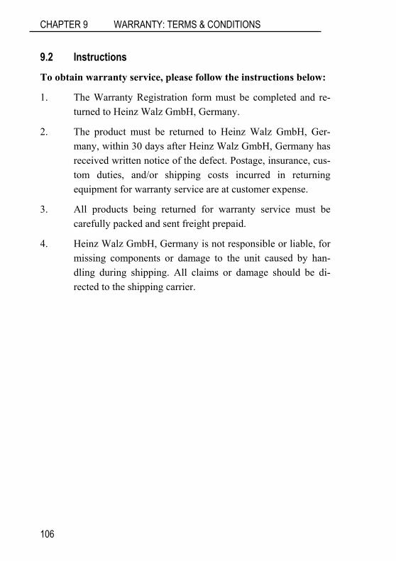
CHAPTER 9 WARRANTY: TERMS & CONDITIONS
9.2 Instructions To obtain warranty service, please follow the instructions below:
1. The Warranty Registration form must be completed and re-turned to Heinz Walz GmbH, Germany.
2. The product must be returned to Heinz Walz GmbH, Ger-many, within 30 days after Heinz Walz GmbH, Germany has received written notice of the defect. Postage, insurance, cus-tom duties, and/or shipping costs incurred in returning equipment for warranty service are at customer expense.
3. All products being returned for warranty service must be carefully packed and sent freight prepaid.
4. Heinz Walz GmbH, Germany is not responsible or liable, for missing components or damage to the unit caused by han-dling during shipping. All claims or damage should be di-rected to the shipping carrier.
106
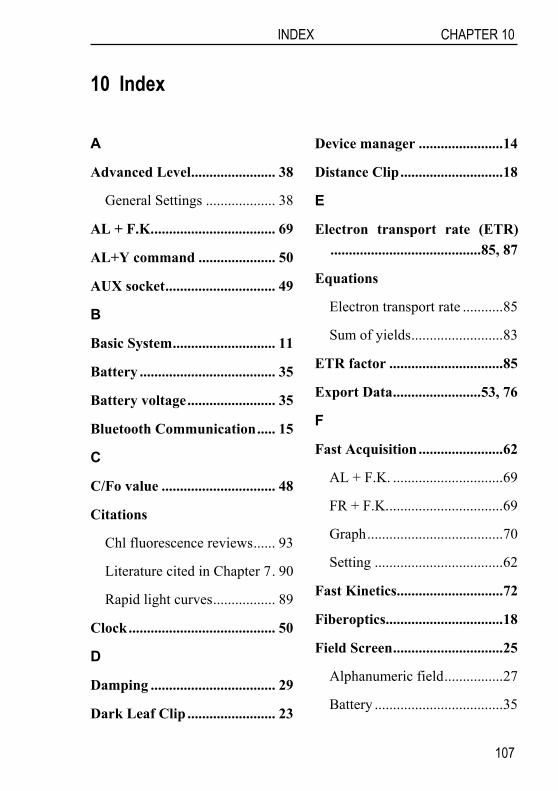
INDEX CHAPTER 10
10 Index
Device manager .......................14 A
Advanced Level....................... 38 Distance Clip............................18
General Settings ................... 38 E
AL + F.K.................................. 69 Electron transport rate (ETR).........................................85, 87 AL+Y command ..................... 50
Equations AUX socket.............................. 49 Electron transport rate ...........85 B Sum of yields.........................83 Basic System............................ 11
ETR factor ...............................85 Battery ..................................... 35 Export Data........................53, 76 Battery voltage........................ 35 F Bluetooth Communication..... 15 Fast Acquisition .......................62 C
AL + F.K. ..............................69 C/Fo value ............................... 48 FR + F.K................................69 Citations Graph.....................................70 Chl fluorescence reviews...... 93 Setting ...................................62 Literature cited in Chapter 7. 90
Fast Kinetics.............................72 Rapid light curves................. 89 Fiberoptics................................18 Clock........................................ 50 Field Screen..............................25 D
Alphanumeric field................27 Damping .................................. 29 Battery ...................................35 Dark Leaf Clip ........................ 23
107
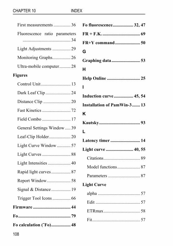
CHAPTER 10 INDEX
First measurements ............... 36 Fo fluorescence.................. 32, 47
Fluorescence ratio parameters.......................................... 34
FR + F.K. ................................. 69
FR+Y command...................... 50 Light Adjustments ................ 29 G Monitoring Graphs................ 26 Graphing data ......................... 53 Ultra-mobile computer.......... 28 H
Figures Help Online ............................. 25
Control Unit .......................... 13 I
Dark Leaf Clip ...................... 24 Induction curve ................. 45, 54
Distance Clip ........................ 20 Installation of PamWin-3....... 13
Fast Kinetics ......................... 72 K
Field Combo ......................... 17 Kautsky.................................... 93
General Settings Window ..... 39 L
Leaf-Clip Holder................... 20 Latency timer .......................... 14
Light Curve Window ............ 57 Light curve ........................ 40, 55
Light Curves ......................... 88 Citations................................ 89
Light Intensities .................... 40 Model functions.................... 87
Rapid light curves ................. 87 Parameters ............................ 87
Report Window..................... 58 Light Curve
Signal & Distance ................. 19 alpha ..................................... 57
Trigger Tool Icons ................ 66 Edit ....................................... 57
Firmware ................................. 44 ETRmax................................ 58
Fo.............................................. 79 Fit.......................................... 57
Fo calculation (˜Fo)................. 48
108
INDEX CHAPTER 10
Ik 58 R
M Rapid light curve .....................40
Measuring light frequency..... 45 Report.......................................58
Micro-Quantum Sensor........ 21, 23 RISC processor........................44
Multiple turn-over flash......... 49 S
N S+H circuit ...............................49
NPQ ......................................... 83 Safety Instructions.....................7
P Saturating Pulse Analysis .......80
PamWin Help.......................... 25 Signal damping ........................29
PAR........................ 21, 35, 41, 85 Single turn-over flash..............49
PAR list.................. 30, 31, 35, 41 Slow kinetics window ..............52
PAR sensor.............................. 47 Software installation ...............13
Polyphasic Rise ....................... 74 Specifications ...........................95
PPFD........................................ 21 T
Pretrigger ................................ 68 Tables
PS I fluorescence..................... 48 Measuring Light Frequency ..45
PAR Lists ..............................40 PS II yield ................................ 33
Trigger.......................64, 66, 68 PWS file ................................... 53
Target Averages.......................64 Q
Temperature ............................41 qL ............................................. 82
Thermocouple ......................22, 23 qN............................................. 83
Trigger qP ............................................. 82
Default...................................74
109

CHAPTER 10 INDEX
Graph .................................... 68
Pretrigger .............................. 68
Settings ................................. 64
Zero Time Shift..................... 69
Trigger pulse ........................... 49
Trouble Shooting .................. 103
U
USB serial port........................ 14
V
View Mode............................... 74
W
Warranty Conditions............ 105
Y
Y(NO)....................................... 83
Y(NPQ) .................................... 83
110