Manual Computational Anatomy Toolbox - CAT12 - uni · PDF fileManual Computational Anatomy...

1

ManualComputationalAnatomyToolbox-CAT12

QUICKSTARTGUIDE.........................................................................................................................3

VERSIONINFORMATION...................................................................................................................5

INTRODUCTIONANDOVERVIEW......................................................................................................6

GETTINGSTARTED............................................................................................................................6DownloadandInstallation 6StartingtheToolbox 7BasicVBManalysis(overview) 7

BASICVBMANALYSIS(DETAILEDDESCRIPTION).............................................................................10

PreprocessingData 10FirstModule:SegmentData 10SecondModule:Displayonesliceforallimages 12ThirdModule:Checksamplehomogeneity 12FourthModule:Smooth 14FifthModule:EstimateTotalIntracranialVolume(TIV) 14

BuildingtheStatisticalModel 15Two-sampleT-Test 16FullFactorialModel(fora2x2Anova) 17MultipleRegression(Linear) 18MultipleRegression(Polynomial) 19

2

FullFactorialModel(Interaction) 20FullFactorialModel(PolynomialInteraction) 21EstimatingtheStatisticalModel 22CheckingforDesignOrthogonality 22DefiningContrasts 24

SPECIALCASES................................................................................................................................29

CAT12forlongitudinaldata 29OptionalChangeofParametersforPreprocessing 31PreprocessingofLongitudinalData 31StatisticalAnalysisofLongitudinalDatainOneGroup 32StatisticalAnalysisofLongitudinalDatainTwoGroups 33

Adaptingtheworkflows 37CustomizedTissueProbabilityMaps 37CustomizedDARTEL-template 38

OTHERVARIANTSOFCOMPUTATIONALMORPHOMETRY..............................................................41

Deformation-basedmorphometry(DBM) 41

Surface-basedmorphometry(SBM) 42

Regionofinterest(ROI)analysis 45

ADDITIONALINFORMATIONONNATIVE,NORMALIZEDANDMODULATEDVOLUMES....................47

NAMINGCONVENTIONOFOUTPUTFILES.......................................................................................48

CALLINGCATFROMTHEUNIXCOMMANDLINE.............................................................................50

TECHNICALINFORMATION.............................................................................................................50

3

Quickstartguide

VBMdata• Segmentdatausingdefaults(useSegmentLongitudinalDataforlongitudinaldata).• EstimateTotalIntracranialVolume(TIV)tocorrectfordifferentheadsizeandvolume.• Check thedataqualitywithCheckSampleHomogeneity forVBMdata (optionally considerTIV

andageasnuisancevariable).• Smoothdata(recommendedstartvalue8mm1).• Specify2nd-levelmodelandcheckfordesignorthogonalityandsamplehomogeneity:

o Use"Fullfactorial"forcross-sectionaldata.o Use"Flexiblefactorial"forlongitudinaldata.o Use TIV as covariate (confound) to correct different brain sizes and select centering

withoverallmean.o Select thresholdmaskingwithanabsolutevalueof0.1.This thresholdcanultimately

beincreasedto0.2oreven0.25.o IfyoufindaconsiderablecorrelationbetweenTIVandanyotherparameterofinterest

itisadvisabletouseglobalscalingwithTIV.Formoreinformation,refertothesection“Buildingthestatisticalmodel”.

• Estimatemodel.• Optionally, Transform SPM-maps to (log-scaled) p-maps or correlation maps and apply

thresholds.• Optionally, you can tryThreshold-FreeCluster Enhancement(TFCE)with the SPM.mat file of a

previouslyestimatedstatisticaldesign.• Optionally,OverlaySelectedSlices.Ifyouareusinglog-pscaledmapsfromTransformSPM-maps

without thresholds, use the following values as the lower range for the colormap for thethresholding:1.3(P<0.05);2(P<0.01);3(P<0.001).

• Optionally, estimate results for ROI analysis usingAnalyze ROIs. Here, the SPM.mat file of apreviouslyestimatedstatisticaldesign isused.Formore information,seetheonlinehelp“AtlascreationandROIbasedanalysis”.

Additionalsurfacedata• Segment data and also select "Surface and thickness estimation" under "Writing options" (for

longitudinaldatauseSegmentLongitudinalData).• Optionally,ExtractAdditional SurfaceParameters (e.g. sulcal depth, gyrification index, cortical

complexity).• Resample& Smooth Surfaces (recommended start value 15mm for cortical thickness and 20-

25mmforfoldingmeasures1,usethedefaultmergingofhemispheres).• CheckdataqualityusingCheckSampleHomogeneityforsurfacedata.• Specify 2nd-level model for (merged) hemispheres and check for design orthogonality and

samplehomogeneity:

4

o Use"Fullfactorial"forcross-sectionaldata.o Use"Flexiblefactorial"forlongitudinaldata.o It isnotnecessary touseTIVasa covariate (confound)becausecortical thicknessor

othersurfacevaluesareusuallynotdependentonTIV.o Itisnotnecessarytousethresholdmasking.o If you find a considerable correlation between a nuisance parameter and any other

parameterofinterestitisadvisabletouseglobalscalingwiththatparameter.Formoreinformation,refertothesection“Buildingthestatisticalmodel”.

• EstimateSurfaceModelfor(merged)hemispheres.• Optionally, Transform SPM-maps to (log-scaled) p-maps or correlation maps and apply

thresholds.• Optionally, you can tryThreshold-FreeCluster Enhancement(TFCE)with the SPM.mat file of a

previouslyestimatedstatisticaldesign.• Optionally,DisplaySurfaceResultsforbothhemispheres.Selecttheresults(preferablysavedas

log-p maps with “Transform and threshold SPM-surfaces”) to display rendering views of yourresults.

• OptionallyExtractROI-basedSurfaceValuessuchas thickness,gyrificationor fractaldimensiontoprovideROIanalysis.

• Optionally, estimate results for ROI analysis usingAnalyze ROIs. Here, the SPM.mat file of apreviouslyestimatedstatisticaldesign isused.Formore information,seetheonlinehelp“AtlascreationandROIbasedanalysis”.

ErrorsduringpreprocessingPlease use theReport Errorfunction if any errors during preprocessing occurred. You first have toselectthe"err"directory,whichis locatedinthefolderofthefailedrecordandfinallythespecifiedzip-fileshouldbeattachedmanuallyinthemail.

AdditionaloptionsAdditional parameters and options are displayed in the CAT12 expertmode. Please note that thismodeisforexperiencedusersonly.1NotetofiltersizesforGaussiansmoothingDuetothehighaccuracyofthespatialregistrationapproachesusedinCAT12youcanalsotrytousesmallerfiltersizesofonlyafewmillimeter.However,forverysmallfiltersizesorevennofilteringyouhavetoapplyanon-parametricpermutationtestsuchastheTFCE-statistics.Please also note that for the analysis of cortical folding measures such as gyrification or corticalcomplexity the filter sizes have to be larger (i.e. in the range of 15-25mm). This is due to theunderlying nature of this measure that reflects contributions from both sulci as well as gyri.Therefore,thefiltersizeshouldexceedthedistancebetweenagyralcrownandasulcalfundus.

5

VersioninformationPreprocessing should remainunaffecteduntil thenextminor versionnumber.AnewprocessingofyourdataisnotnecessaryiftheminorversionnumberofCAT12remainsunchanged.

ChangesinversionCAT12.3(1300)• Changesinpreprocessingpipeline(whichaffectsyourresultscomparedtoCAT12.2)

o Skull-strippingisagainslightlychangedandtheSPMapproachisnowusedasdefault.TheSPMapproachworksquitestable for themajorityofdata.However, insomerarecasespartsofGM(i.e.infrontallobe)mightbecut.IfthishappenstheGCUTapproachisagoodalternative.

o Spatial adaptivenon-localmean (SANLM) filter is again calledas very first stepbecausenoiseestimationandde-noisingworksbestfororiginal(non-interpolated)data.

o Corticalthicknessestimationisnowcorrectedusingpialandwhitemattersurface.Thesetwo surfaces are created initially using central surface and cortical thickness and thepositioniscorrectedinregionswithself-intersections.

ChangesinversionCAT12.2(1290)• Changesinpreprocessingpipeline(whichaffectsyourresultscomparedtoCAT12.1)

o Skull-strippingnowadditionally uses SPM12 segmentations by default: Thedefault gcutapproachinCAT12.1removedtoomuchofthesurrounding(extracranial)CSF,whichledtoaslightunderestimationofTIVforatrophiedbrains.Theskull-strippingapproachbasedon the SPM12 segmentations prevents this through a more conservative approach.However,sometimespartsofthemeninges(i.e.duramater)orothernon-brainpartsstillremain in the GM segmentation. By combining both approaches a more reliable skull-strippingisachieved.

o MorereliableestimationofTIV:Thechangedskull-strippingalsoaffectsestimationofTIV,whichisnowmorereliable,especiallyforatrophiedbrains.

• Importantnewfeatureso Automatic check for design orthogonality and sample homogeneity using SPM.mat in

BasicModelso Addedequi-volumemodelbyBokandmulti-saveoption formappingnativevolumes to

individualsurfaceso Added Local-Global Intrinsic Functional Connectivity parcellation by Schaefer et al. for

resting-statefMRIdata

6

IntroductionandOverviewThismanual is intended to help any user to perform a computational anatomy analysis using theCAT12 Toolbox. Although it mainly focuses on voxel-based morphometry (VBM) other variants ofcomputationalanalysissuchasdeformation-basedmorphometry(DBM),surface-basedmorphometry(SBM),andregionofinterest(ROI)morphometricanalysisarealsopresentedandcanbeappliedwithfewchanges.

Basically,themanualcanbedividedintofourmainsections:

• Naturally, a quick guide of how to get started is given at the beginning. This section providesinformationaboutdownloadingandinstallingthesoftwareandstartingtheToolbox.Inaddition,abriefoverviewofthestepsofaVBManalysisisgiven.

• ThisisfollowedbyadetaileddescriptionofabasicVBManalysisthatguidestheuserstep-by-stepthrough the entire process – from preprocessing to contrast selection. This description shouldprovidealltheinformationnecessarytosuccessfullyanalyzemoststudies.

• TherearesomespecificcasesofVBManalyses,forwhichthebasicanalysisworkflowneedstobeadapted.Thesecasesarelongitudinalstudiesandstudiesinchildrenorspecialpatientpopulations.RelevantchangestoabasicVBManalysisaredescribedhereandhowtoapplythesechanges.Itisimportantthatonlythechangesaredescribed–stepssuchasqualitycontrolorsmoothingarethesameasthosedescribedinthebasicanalysisandnotrepeatedasecondtime.

• The guide concludes with information about native, normalized and modulated volumes thatdeterminehowtheresultscanbeinterpreted.Inaddition,anoverviewofthenamingconventionsusedandtechnicalinformationisgiven.

GettingStartedDOWNLOADANDINSTALLATION• The CAT12 Toolbox runs within SPM12. That is, SPM12 must be installed and added to your

Matlab search path before the CAT12 Toolbox can be installed (seehttp://www.fil.ion.ucl.ac.uk/spm/andhttp://en.wikibooks.org/wiki/SPM).

• Download (http://dbm.neuro.uni-jena.de/cat12/) and unzip the CAT12 Toolbox. You will get afoldernamed“cat12”,whichcontainsvariousMatlabfilesandcompiledscripts.Copythefolder“cat12”intotheSPM12“toolbox”folder.

7

STARTINGTHETOOLBOX• StartMatlab• StartSPM12(i.e.,type“spmfmri”)• Select“cat12”fromtheSPMmenu(seeFigure1).Youwillfindthedrop-downmenubetweenthe

“Display”andthe“Help”button(youcanalsocalltheToolboxdirectlybytyping“cat12”ontheMatlabcommandline).ThiswillopentheCAT12Toolboxasadditionalwindow(Fig.2).

Figure1:SPMmenu Figure2:CAT12Window

BASICVBMANALYSIS(OVERVIEW)TheCAT12Toolboxcomeswithdifferentmodules,whichmaybeusedforananalysis.Usually,aVBManalysiscomprisesthefollowingsteps

(a)Preprocessing:

1. T1 imagesarenormalizedtoatemplatespaceandsegmented intograymatter(GM),whitematter(WM)andcerebrospinalfluid(CSF).Thepreprocessingparameterscanbeadjustedviathemodule“SegmentData”.

2. After the preprocessing is finished, a quality check is highly recommended. This can beachievedviathemodules“Displayonesliceforallimages”and“Checksamplehomogeneity”.

8

Both options are located in the CAT12 window under “Check Data Quality”. Furthermore,quality parameters are estimated and saved in xml-files for each data set duringpreprocessing.ThesequalityparametersarealsoprintedonthereportPDF-pageandcanbeadditionallyusedinthemodule“Checksamplehomogeneity”.

3. BeforeenteringtheGMimagesintoastatisticalmodel,imagedataneedtobesmoothed.Ofnote,thisstepisnotimplementedintotheCAT12ToolboxbutachievedviathestandardSPMmodule“Smooth”.

(b)Statisticalanalysis:

4. The smoothed GM images are entered into a statistical analysis. This requires building astatistical model (e.g. T-Tests, ANOVAs, multiple regressions). This is done by the standardSPMmodules“Specify2ndLevel”or“BasicModels”intheCAT12windowcoveringthesamefunction.

5. The statistical model is estimated. This is done with the standard SPMmodule “Estimate”(exceptforsurface-baseddatawherethefunction“EstimateSurfaceModels”shouldbeusedinstead).

6. If you have used total intracranial volume (TIV) as confound in your model to correct fordifferent brain sizes it is necessary to checkwhether TIV reveals a considerable correlationwithanyotherparameterofinterestandratheruseglobalscalingasalternativeapproach.

7. Afterestimatingthestatisticalmodel,contrastsaredefinedtogettheresultsoftheanalysis.ThisisdonewiththestandardSPMmodule“Results”.

Thesequenceof“preprocessingà qualitycheckà smoothingà statisticalanalysis”remainsthesameforeveryVBManalysis,evenwhendifferentstepsareadapted(see“specialcases”).AfewwordsabouttheBatchEditor…

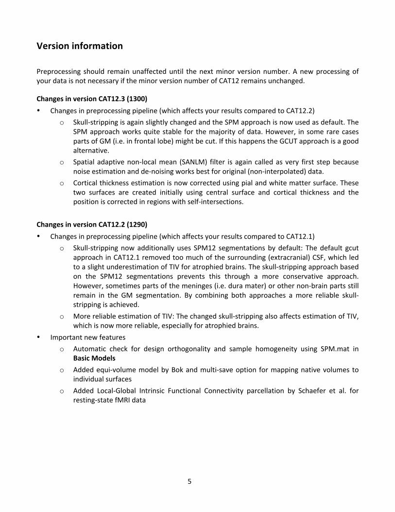
− As soon as you select amodule from the CAT12 Toolboxmenu, a newwindow (the BatchEditor)willopen.TheBatchEditoristheenvironmentwhereyouwillsetupyouranalysis(seeFigure3).Forexample,an“<-X”indicateswhereyouneedtoselectfiles(e.g.yourimagefiles,thetemplate,etc.).Otherparametershaveeitherdefaultsettings(whichcanbemodified)orrequireinput(e.g.choosingbetweendifferentoptions,providingtextornumericvalues,etc.).

− Onceallmissingparametersareset,agreenarrowwillappearonthetopofthewindow(thecurrentsnapshotsinFigure3showthearrowstillingray).Clickthisarrowtorunthemoduleor select “FileàRunBatch”. It is veryuseful to save thesettingsbeforeyou run thebatch(clickonthedisksymbolorselect“FileàSaveBatch”).

− Ofnote,youcanalways findhelpful informationandparameter-specificexplanationsat thebottomoftheBatchEditorwindow.1

1AdditionalCAT12-relatedinformationcanbefoundbyselecting“VBMWebsite“intheCAT12window(Tools→Internet→VBMWebsite”).Thiswillopenawebsite.Here,lookfor“VBMsubpages”ontheright.

9

− Allsettingscanbesavedeitheras.matfileoras.mscriptfileandreloadedforlateruse.The.mscriptfilehastheadvantagetobeeditablewithatexteditor.

Figure 3: The Batch Editor is the environment where the analysis is set up. Left: For all settingsmarkedwith “<-X”, files have to be selected (“Select Files”).Right: Parameters can be edited andadapted(“EditValue”).

10

BasicVBMAnalysis(detaileddescription)

PreprocessingData

FIRSTMODULE:SEGMENTDATA

PleasenotethatadditionalparametersforexpertusersaredisplayedintheGUIifyousettheoptioncat.extopts.expertguito“1”incat_defaults.morcallcat12by:

cat12(‘expert’)

CAT12àPreprocessingàSegmentData

Parameters:

o Volumes<-XàSelectFilesà[selectthenewfiles]àDone

- Selectonevolumeforeachsubject.AstheToolboxdoesnotsupportmultispectraldata(i.e.,differentimagingmethodsforthesamebrain,suchasT1-,T2-,diffusion-weightedorCTimages),itisrecommendedtochooseaT1-weightedimage.

- Importantly,theimagesneedtobeinthesameorientationasthepriors;youcandouble-check and correct via using “Display” in the SPM menu. The priors arelocatedinyourSPMfolder“SPM12àtpmàTPM.nii”)

o Splitjobintoseparateprocessesà[usedefaultsormodify]- Tousemulti-threadingtheCAT12segmentationjobwithmultiplesubjectscanbe

split into separate processes that run in the background. You can even closeMatlab,whichwillnotaffecttheprocessesthatwillruninthebackgroundwithoutGUI.Ifyoudon’twanttorunprocessesinthebackgroundthensetthisvalueto0.

- Keep inmind that eachprocess needs about 1.5..2GBof RAM,which should beconsideredtochoosetheappropriatenumberofprocesses.

- Please further note that no additional modules in the batch can be run exceptCAT12segmentation.Anydependenciesarebrokenforsubsequentmodules.

o OptionsforinitialSPM12affineregistrationà[usedefaultsormodify]- The defaults provide a solid starting point. The SPM12 tissue probability maps

(TPMs)areusedfortheinitialspatialregistrationandsegmentation.Alternatively,customizedTPMscanbechosen(e.g.forchildrendata)thatwerecreatedwiththeTemplate-O-Matic(TOM)Toolbox.

o ExtendedoptionsforCAT12segmentationà[usedefaultsormodify]

- Again,thedefaultsprovideasolidstartingpoint.Usingtheextendedoptionsyoucanadjustspecificparametersorthestrengthofdifferentcorrections("0"means

11

nocorrectionand"0.5" isthedefaultvaluethatworksbestfora largevarietyofdata).

- CAT12 provides a template for the high-dimensional DARTEL registration thatshould work for most data. However, a customized DARTEL template can beselected (e.g. for childrendata) thatwas createdusing theDARTEL toolbox. Formore information on the necessary steps, see the section "Customized DARTELTemplate".

o Writingoptionsà[usedefaultsormodify]

- ForGM, andWM image volumes see at the end of the document: “Additionalinformationonnative,normalizedandmodulatednormalizedvolumes”.Note:Thedefaultoption“Modulatednormalized”resultsinananalysisofrelativedifferencesin regionalGMvolume, thathave tobe corrected for individualbrain size in thestatisticalanalysisusingtotalintracranialvolume(TIV).

- A Bias, noise and globally intensity corrected T1 image, in which MRIinhomogeneities and noise are removed and intensities are globally normalized,canbewritten innormalized space.This isuseful forquality control andalso tocreate an average image of all normalized T1 images to display / overlay theresults.Note:ForabasicVBManalysisusethedefaults.

- A partial volume effect (PVE) label image volume can also be written innormalized or native space or as a DARTEL export file. This is useful for qualitycontrol andalso for futureapplicationsusing this image to reconstruct surfaces.Note:ForabasicVBManalysisusethedefaults.

- TheJacobiandeterminantforeachvoxelcanbewritteninnormalizedspace.ThisinformationcanbeusedtodoaDeformation-BasedMorphometry(DBM)analysis.Note:ForabasicVBManalysisthisisnotneeded.

- Finally, deformation fields can be written. This option is useful to re-applynormalization parameters to other co-registered images (e.g. fMRI or DTI data).Note:ForabasicVBManalysisthisisnotneeded.

Note:Ifthesegmentationfails,thisisoftenduetoanunsuccessfulinitialspatialregistration.Inthiscase,youcantrytosettheorigin(anteriorcommissure)intheDisplaytool.Placethecursorroughlyontheanteriorcommissureandpress“SetOrigin”Thenowdisplayedcorrection inthecoordinatescanbeappliedtothe imagewiththebutton“Reorient”.Thisproceduremustberepeatedforeachdatasetindividually.

12

SECONDMODULE:DISPLAYONESLICEFORALLIMAGES

CAT12àCheckdataqualityàDisplayonesliceforallimages

Parameters:

o Sampledata<-XàSelectFilesà[selectthenewfiles]àDone

- Selectthenewlywrittendata[e.g.the“wm*”files,whicharethenormalizedbiascorrectedvolumes].Thistoolwilldisplayonehorizontalsliceforeachsubject,thusgivingagoodoverviewifthesegmentationandnormalizationproceduresyieldedreasonableresults.Forexample,ifthenativevolumehadartifactsorifthenativevolumeshadawrongorientation,theresultsmaylookodd.Solutions:Use“CheckReg”fromtheSPMmainmenutomakesurethatthenativeimageshavethesameorientationliketheMNITemplate(“SPMàtemplatesàT1”).Adjustifnecessaryusing“Display”fromtheSPMmainmenu.

o Proportionalscalingà[usedefaultsormodify]- Check“yes”,ifyoudisplayT1volumes.

o Spatialorientationo Showsliceinmmà[usedefaultsormodify]

- This module displays horizontal slices. This default setting provides a goodoverview.

THIRDMODULE:CHECKSAMPLEHOMOGENEITY

CAT12àCheckdataqualityàChecksamplehomogeneityàVBMdata

Parameters:

o DataàNew:Sampledata<-XàSelectFilesà[selectgraymattervolumes]àDone- Selectthenewlywrittendata[e.g.the“mwp1*”files,whicharethemodulated(m)

normalized (w) GM segments (p1)]. It is recommended to use the unsmoothedsegmentations that provide more anatomical details. This tool visualizes thecorrelationbetweenthevolumesusingaboxplotandcorrelationmatrices.Thus,itwillhelpidentifyingoutliers.Anyoutliershouldbecarefullyinspectedforartifactsor pre-processing errors using “Check worst data” in the GUI. If you specifydifferentsamplesthemeancorrelationisdisplayedinseparateboxplotsforeachsample.

o Loadqualitymeasures(optional)à[optionallyselectxml-fileswithqualitymeasures]- Optionallyselectthexml-filesthataresavedforeachdataset.Thesefilescontain

usefulinformationaboutsomeestimatedqualitymeasuresthatcanbealsoused

13

forcheckingsamplehomogeneity.Pleasenote,thattheorderofthexml-filesmustbethesameastheotherdatafiles.

o Separationinmmà[usedefaultsormodify]- Tospeedupcalculationsyoucandefinethatcorrelationisestimatedonlyeveryx

voxel.Smallervaluesgiveslightlymoreaccuratecorrelation,butaremuchslower.o Nuisanceà[enternuisancevariablesifapplicable]

- For each nuisance variable which you want to remove from the data prior tocalculating the correlation, select “New: Nuisance” and enter a vector with therespective variable for each subject (e.g. age in years). All variables have to beentered in the same order as the respective volumes. You can also type“spm_load” to upload a *txt file with the covariates in the same order as thevolumes.ApotentialnuisanceparametercanbeTIVifyouchecksegmenteddatawiththedefaultmodulation.

Awindowopenswithacorrelationmatrixinwhichthecorrelationbetweenthevolumesisdisplayed.Thecorrelationmatrixshowsthecorrelationbetweenallvolumes.Highcorrelationvaluesmeanthatyourdataaremoresimilartoeachother.Ifyouclickinthecorrelationmatrix,thecorrespondingdatapairs are displayed in the lower right corner and allow a closer look. The slider below the imagechangesthedisplayedslice.Thepop-pupmenusinthetopright-handcornerprovidemoreoptions.Hereyoucanselectothermeasuresthataredisplayedintheboxplot(e.g.optionalqualitymeasuressuchasnoise,bias,weightedoverall imagequality if thesevaleswere loaded),changetheorderofthecorrelationmatrix(accordingtofilenameormeancorrelation).Finally,themostdeviatingdatacanbedisplayedintheSPMgraphicswindowtocheckthedatamoreclosely.Theboxplot intheSPMgraphicswindowaveragesallcorrelationvaluesforeachsubjectandshowsthehomogeneityofyoursample.Asmalloverallcorrelationintheboxplotnotalwaysmeansthatthisvolume is anoutlier or contains an artifact. If there are no artifacts in the image and if the imagequalityisreasonableyoudon’thavetoexcludethisvolumefromthesample.Thistoolisintendedtoutilizetheprocessofqualitycheckingandthereisnoclearcriteriadefinedtoexcludeavolumeonlybasedontheoverallcorrelationvalue.However,volumeswithanoticeableloweroverallcorrelation(e.g.belowtwostandarddeviations)areindicatedandshouldbecheckedmorecarefully.If you have loaded qualitymeasures, you can also display theMahalanobis distance between twomeasures:meancorrelationandweightedoverall imagequality.Thesetwoarethemost importantmeasuresforassessingimagequality.Meancorrelationmeasuresthehomogeneityofyourdatausedfor statistical analysis and is therefore ameasure of image quality after pre-processing. Data thatdeviatefromyoursampleincreasevarianceandthereforeminimizeeffectsizeandstatisticalpower.Theweightedoverallimagequality,ontheotherhand,combinesmeasurementsofnoiseandspatialresolution of the images before pre-processing. Although CAT12 uses effective noise-reductionapproaches(e.g.spatialadaptivenon-localmeansfilter)pre-processedimagesarealsoaffectedandshouldbechecked.TheMahalanobisdistancemakesitpossibletocombinethesetwomeasuresofimagequalitybeforeandafterpre-processing.IntheMahalanobisplot,thedistanceiscolor-codedandeachpointcanbeselectedtogetthefilenameanddisplaytheselectedslicetocheckdatamoreclosely.

14

FOURTHMODULE:SMOOTH

SPMmenuàSmooth

Parameters:

o ImagestoSmooth<-XàSelectFilesà[selectgreymattervolumes]àDone- Select the newly written data [e.g. the “mwp1” files, which are the

modulated(m)normalized(w)greymattersegments(p1)].

o FWHMà[usedefaultsormodify]- 8-12mmkernelsarewidelyusedforVBM.Tousethissettingselect“edit

value”andtype“888”(or“121212”,respectively)forakernelwith8mm(with12mm)FWHM.

o DataTypeà[usedefaultsormodify]

o FilenamePrefixà[usedefaultsormodify]

FIFTHMODULE:ESTIMATETOTALINTRACRANIALVOLUME(TIV)

CAT12àStatisticalAnalysisàEstimateTIV

Parameters:

o XMLfiles<-XàSelectFilesà[selectxml-files]àDone- Selectthexml-filesinthereport-folder[e.g.the“cat_*.xml”].

o SavevaluesàTIVonly- ThisoptionwillsavetheTIVvaluesforeachdatasetinthesameorderas

the selected xml-files.Optionally you can also save the global values foreachtissueclass,whichmightbeinterestingforfurtheranalysis,butisnotrecommendedifyouareinterestedinonlyusingTIVascovariate.

o Outputfileà[usedefaultsormodify]

PleasenotethatTIVisstronglyrecommendedascovariateforallVBManalysistocorrectdifferentbrainsizes.Thisstepisnotnecessaryfordeformation-orsurface-baseddata.PleasealsomakesurethatTIVdoesnotcorrelatetoomuchwithyourparametersofinterest(pleasemakesurethatyouuse “Centering” with “Overall mean”, otherwise the check for orthogonality in SPM sometimesdoesnotworkcorrectly).InthiscaseyoushoulduseglobalscalingwithTIV.

15

BuildingtheStatisticalModelAlthough many potential designs are offered in 2nd-level analysis I recommend using the “Fullfactorial”designas itcoversmoststatisticaldesigns.Forcross-sectionalVBMdatayouusuallyhave1..nsamplesandoptionallycovariatesandnuisanceparameters:Numberoffactorlevels Numberofcovariates StatisticalModel1 0 one-samplet-test1 1 singleregression1 >1 multipleregression2 0 two-samplet-test>2 0 Anova

>1 >0 AnCova (for nuisance parameters) orInteraction(forcovariates)

16

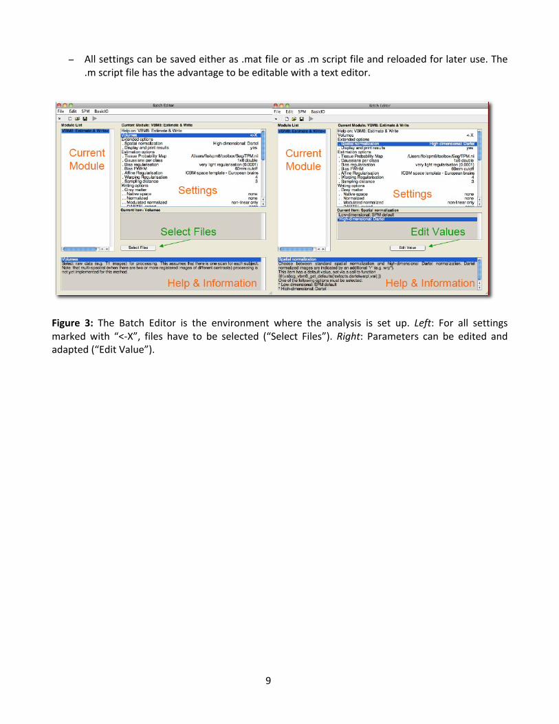
TWO-SAMPLET-TEST

CAT12→StatisticalAnalysis→BasicModels

Parameters:

o Directory <-Xà Select Filesà [select theworkingdirectoryforyouranalysis]àDone

o Designà“Two-samplet-test”§ Group 1 scans à Select Files à

[select the smoothed grey mattervolumes for group 1; following thisscriptthesearethe“smwp1”files]àDone

§ Group 2 scans à Select Files à[select the smoothed grey mattervolumesforgroup2]àDone

§ IndependenceàYes§ VarianceàEqualorUnequal§ GrandmeanscalingàNo§ ANCOVAàNo

o Covariates*(seetextbox)

o Masking§ ThresholdMaskingàAbsoluteà[specifyvalue(e.g.“0.1”)]§ ImplicitMaskàYes§ ExplicitMaskà<None>

o GlobalCalculationàOmit

o GlobalNormalization§ OverallgrandmeanscalingàNo

o NormalizationàNone

*You could specify one or more covariates (i.e.,partial out the variance of specific factors whenlookingatgroupdifferences).It is strongly recommended to always use totalintracranial volume (TIV) as covariate formodulated data in VBM to correct different brainsizes.ThisisnotnecessaryforsurfaceanalysisandDBM.

• CovariatesàNewCovariate

• Vector <-X à enter the values of thecovariates (e.g. TIV and optionally age inyears)inthesameorderastherespectivefilenames or type “spm_load” to upload a *.txtfilewith thecovariates in the sameorderasthevolumes

• Name<-XàSpecifyText(e.g.“age”)

• InteractionsàNone

• CenteringàOverallmean

17

FULLFACTORIALMODEL(FORA2X2ANOVA)


Parameters:

o Directory<-XàSelectFilesà[selecttheworkingdirectoryforyouranalysis]àDoneo Designà“FullFactorial”

§ Factorsà“New:Factor;New:Factor”Factor• Nameà[specifytext(e.g.”sex”)]• Levelsà2• IndependenceàYes• VarianceàEqualorUnequal• GrandmeanscalingàNo• ANCOVAàNoFactor• Nameà[specifytext(e.g.“handedness”)]• Levelsà2• IndependenceàYes• VarianceàEqualorUnequal• GrandmeanscalingàNo• ANCOVAàNo

§ SpecifyCellsà“New:Cell;New:Cell;New:Cell;New:Cell”Cell• Levelsà[specifytext(e.g.“11”)]• Scansà[selectfiles(e.g.thesmoothedGMvolumesoftheleft-handedmales)]Cell• Levelsà[specifytext(e.g.“12”)]• Scansà[selectfiles(e.g.thesmoothedGMvolumesoftheright-handedmales)]Cell• Levelsà[specifytext(e.g.“21”)]• Scansà[selectfiles(e.g.thesmoothedGMvolumesoftheleft-handedfemales)]Cell• Levelsà[specifytext(e.g.“22”)]• Scansà[selectfilese.g.thesmoothedGMvolumesoftheright-handedfemales)]

o Covariates*(seetextboxinexamplefortwo-sampleT-test)





18

MULTIPLEREGRESSION(LINEAR)


Parameters:

o Directory<-XàSelectFilesà[selectthedirectoryforyouranalysis]àDone

o Designà“MultipleRegression”§ Scansà[selectfiles(e.g.thesmoothedGMvolumesofallsubjects)]àDone§ Covariatesà“New:Covariate”

Covariate

• Vectorà [enter the values in the same order as the respective file names of thesmoothedGMimages]

• Nameà[specifytest(e.g.“age”)]• CenteringàOverallmean

§ InterceptàIncludeIntercepto Covariates*(seetextboxinexamplefortwo-sampleT-test)o Masking

§ ThresholdMaskingàAbsoluteà[specifyvalue(e.g.“0.1”)]§ ImplicitMaskàYes§ ExplicitMaskà<None>



o NormalizationàNon

19

MULTIPLEREGRESSION(POLYNOMIAL)

Touseapolynomialmodel,youneedtoestimatethepolynomialfunctionofyourparameterbeforeanalyzingit.Todothis,usethefunctioncat_stat_polynomial(includedwithCAT12>r1140):

y=cat_stat_polynomial(x,order)

where“x”isyourparameterand“order”isthepolynomialorder(e.g.2forquadratic).

Exampleforpolynomialorder2(quadratic):


Parameters:

o Directory<-XàSelectFilesà[selectthedirectoryforyouranalysis]àDone

o Designà“MultipleRegression”§ Scansà[selectfiles(e.g.thesmoothedGMvolumesofallsubjects)]àDone§ Covariatesà“New:Covariate”

Covariate• Vectorà[specifylinearterm(e.g.“y(:,1)”)]• Nameà[specifytest(e.g.“agelinear”)]• CenteringàOverallmean

§ Covariatesà“New:Covariate”Covariate• Vectorà[specifyquadraticterm(e.g.“y(:21)”)]• Nameà[specifytest(e.g.“agequadratic”)]• CenteringàOverallmean

§ InterceptàIncludeIntercepto Covariates*(seetextboxinexamplefortwo-sampleT-test)o Masking





20

FULLFACTORIALMODEL(INTERACTION)


Parameters:


§ Factorsà“New:Factor”Factor• Nameà[specifytext(e.g.”sex”)]• Levelsà2• IndependenceàYes• VarianceàEqualorUnequal• GrandmeanscalingàNo• ANCOVAàNo

§ SpecifyCellsà“New:Cell;New:Cell”Cell• Levelsà[specifytext(e.g.“1”)]• Scansà[selectfiles(e.g.thesmoothedGMvolumesofthemales)]Cell• Levelsà[specifytext(e.g.“2”)]• Scansà[selectfiles(e.g.thesmoothedGMvolumesofthefemales)]

o Covariatesà“New:Covariate”§ Covariate

• Vectorà [enter the values in the same order as the respective file names of thesmoothedGMimages]

• Nameà[specifytest(e.g.“age”)]• InteractionsàWithFactor1• CenteringàOverallmean

o Covariates*(seetextboxinexamplefortwo-sampleT-test)o Masking





21

FULLFACTORIALMODEL(POLYNOMIALINTERACTION)

To use a polynomial model you have to estimate the polynomial function of your parameter prior to theanalysis.Usethefunctioncat_stat_polynomial(providedwithCAT12>r1140)forthatpurpose:

y=cat_stat_polynomial(x,order)

where“x”isyourparameterand“order”isthepolynomialorder(e.g.2forquadratic).

Exampleforpolynomialorder2(quadratic):


Parameters:


§ Factorsà“New:Factor”Factor• Nameà[specifytext(e.g.”sex”)]• Levelsà2• IndependenceàYes• VarianceàEqualorUnequal• GrandmeanscalingàNo• ANCOVAàNo

§ SpecifyCellsà“New:Cell;New:Cell”Cell• Levelsà[specifytext(e.g.“1”)]• Scansà[selectfiles(e.g.thesmoothedGMvolumesofthemales)]Cell• Levelsà[specifytext(e.g.“2”)]• Scansà[selectfiles(e.g.thesmoothedGMvolumesofthefemales)]


• Vectorà[specifylinearterm(e.g.“y(:,1)”)]• Nameà[specifytest(e.g.“agelinear”)]• InteractionsàWithFactor1• CenteringàOverallmean


• Vectorà[specifyquadraticterm(e.g.“y(:,2)”)]• Nameà[specifytest(e.g.“agequadratic”)]• InteractionsàWithFactor1• CenteringàOverallmean

o Covariates*(seetextboxinexamplefortwo-sampleT-test)o Masking

§ ThresholdMaskingàAbsoluteà[specifyvalue(e.g.“0.1”)]§ ImplicitMaskàYes

22

§ ExplicitMaskà<None>




ESTIMATINGTHESTATISTICALMODEL

SPMmenuàEstimate

Parameters:

o SelectSPM.mat<-XàSelectFilesà[selecttheSPM.matwhichyoujustbuilt]àDone

o Methodà“Classical”

CHECKINGFORDESIGNORTHOGONALITY

If youhavemodeled TIV as confoundingparameter, youmust checkwhether TIV is orthogonal (inotherwords independent) toanyotherparameterof interest inyouranalysis (e.g.parametersyouare testing for). This means that TIV should not correlate with any other parameter of interest,otherwisenotonly the varianceexplainedbyTIV is removed fromyourdata,but alsopartsof thevarianceofyourparameterofinterest.Pleaseuse“Overallmean”as“Centering”fortheTIVcovariate.Otherwise,theorthogonalitychecksometimesevenindicatesameaningfulco-linearityonlybecauseofscalingproblems.Tocheckthedesignorthogonality,youcanusetheReviewfunctionintheSPMGUI:SPMmenuàReview

o SelectSPM.mat<-XàSelectFilesà[selecttheSPM.matwhichyoujustbuilt]àDone

o DesignàDesignorthogonality

23

Figure4:Grayboxesbetweentheparameterspointtoaco-linearity(correlation):thedarkertheboxthe larger the correlation (whichalsoholds for inverse correlations). If youclick in thebox the co-linearitybetweentheparametersisdisplayed.

ThelargerthecorrelationbetweenTIVandanyparameterofinterestthemoretheneedtonotuseTIVasnuisanceparameter.InthiscaseanalternativeapproachistouseglobalscalingwithTIV.Usethefollowingsettingsforthisapproach:

o GlobalCalculationàUseràGlobalValues<-XàDefinetheTIVvalueshereo GlobalNormalisationàOverallgrandmeanscalingàYesàGrandmeanscaledvalue

àDefineherethemeanTIVofyoursampleor(orasapproximationavalueof1500whichmightfitforthemajorityofdatafromadults)

o Normalisation• Approach1(forallmodels):NormalizationàProportional

• Approach2(forallmodelswithmorethanonegroup):NormalizationàANCOVA

24

Approach 1 is (proportionally) scaling the data according to the individual TIV values. Instead ofremovingvarianceexplainedbyTIValldataarescaledbytheirTIVvalues.This isalsosimilartotheapproachthatwasused inVBM8(“modulatefornon-lineareffectsonly”),whereglobalscalingwasinternallyusedwithanapproximationofTIV(e.g.inverseofaffinescalingfactor).Thisapproachcanbeusedforallmodelsincludingmultipleregressionswithonegroup.Approach2isusingTIVasnuisanceparameterwithseparatecolumnsforeachgroup.Thevaluesforthe nuisance parameters are heremean-centered for each group. As themean values for TIV arecorrected separately for each group, it is prevented that group differences in TIV have a negativeimpact on the group comparison of the image data in theGLM. Variance explained by TIV is hereremovedseparatelyforeachgroup.PleasenotethatthisapproachisalsoequivalenttotheuseofTIVas nuisance parameter with interaction and mean centering with factor “group”. The design alsoresultsinseparatecolumnsforTIV,whicharemean-correctedforeachgroup.Unfortunately,anoclearadviceforeitherofthesetwoapproachescanbegivenandtheuseoftheseapproacheswillalsoaffectinterpretationofyourfindings.Pleasenotethatglobalnormalizationalsoaffectstheabsolutemaskingthresholdasyourimagesarenowscaledtothe“Grandmeanscaledvalue”oftheGlobalNormalizationoption.Ifyouhavedefinedthemean TIV of your sample (or an approximate value of 1500) here, no change of the absolutethresholdisrequired.Otherwise,youwillhavetocorrecttheabsolutethresholdbecauseyourvaluesarenowgloballyscaledtothe“Grandmeanscaledvalue”oftheGlobalNormalizationoption.

DEFININGCONTRASTS

SPMmenuà Resultsà [select the SPM.mat file]à Done (this opens the ContrastManager)àDefinenewcontrast(i.e.,choose“t-contrast”or“F-contrast”;typethecontrastnameandspecifythecontrastbytypingtherespectivenumbers,asshownbelow):Pleasenot thatall zerosat theendof the contrastdon’thave tobedefined,butare sometimesremainedfordidacticreasons.

Contrasts:

Two-sampleT-test

T-test

• ForGroupA>GroupB

• ForGroupA<GroupB:

1-1-11

F-test

• ForanydifferencesbetweenGroupAandB:

1-1

25

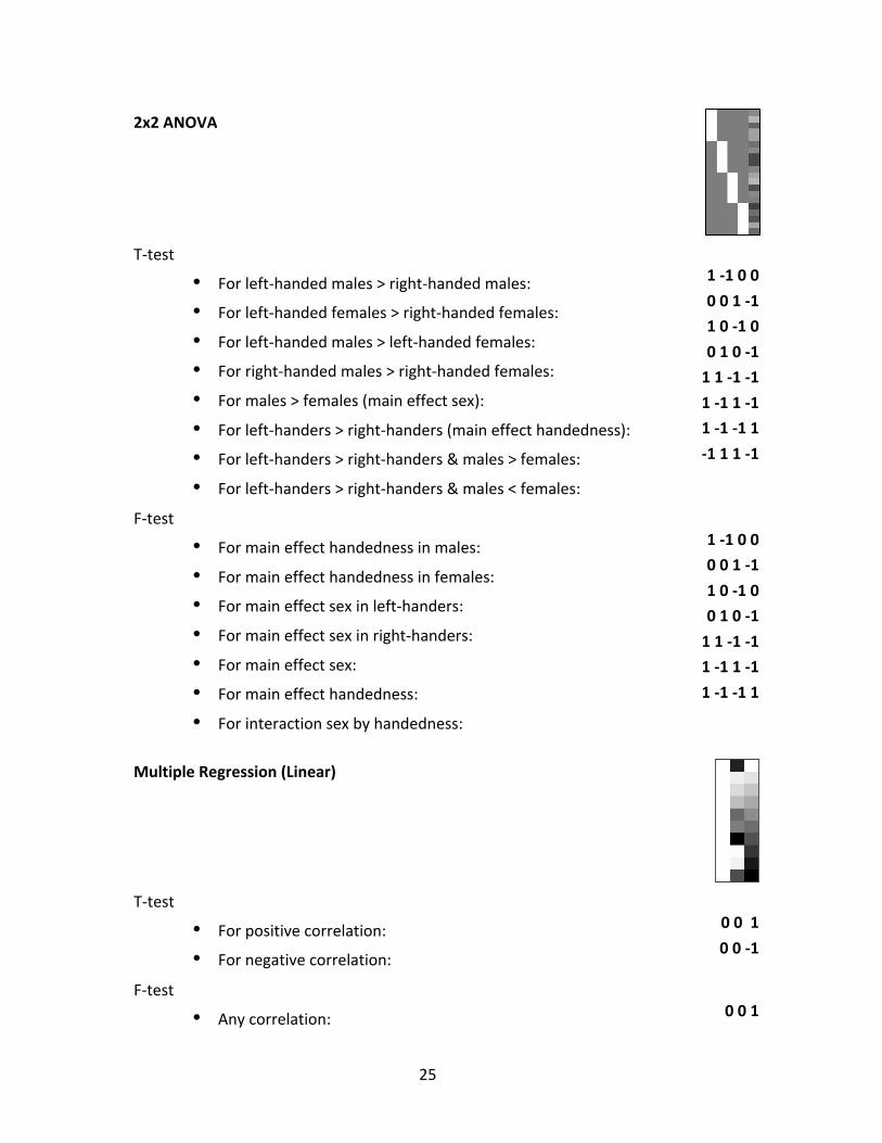
2x2ANOVA

T-test

• Forleft-handedmales>right-handedmales:

• Forleft-handedfemales>right-handedfemales:

• Forleft-handedmales>left-handedfemales:

• Forright-handedmales>right-handedfemales:

• Formales>females(maineffectsex):

• Forleft-handers>right-handers(maineffecthandedness):

• Forleft-handers>right-handers&males>females:

• Forleft-handers>right-handers&males<females:

1-100001-110-10010-111-1-11-11-11-1-11-111-1

F-test

• Formaineffecthandednessinmales:

• Formaineffecthandednessinfemales:

• Formaineffectsexinleft-handers:

• Formaineffectsexinright-handers:

• Formaineffectsex:

• Formaineffecthandedness:

• Forinteractionsexbyhandedness:

1-100001-110-10010-111-1-11-11-11-1-11

MultipleRegression(Linear)

T-test

• Forpositivecorrelation:

• Fornegativecorrelation:

00100-1

F-test

• Anycorrelation:

001

26

Thetwoleadingzerosincontrastindicatetheconstant(sampleeffect,1stcolumninthedesignmatrix)andTIV(2ndcolumninthedesignmatrix). IfnoadditionalcovariatesuchasTIV isdefinedyoumustskiponeoftheleadingzeros(e.g.“01”).

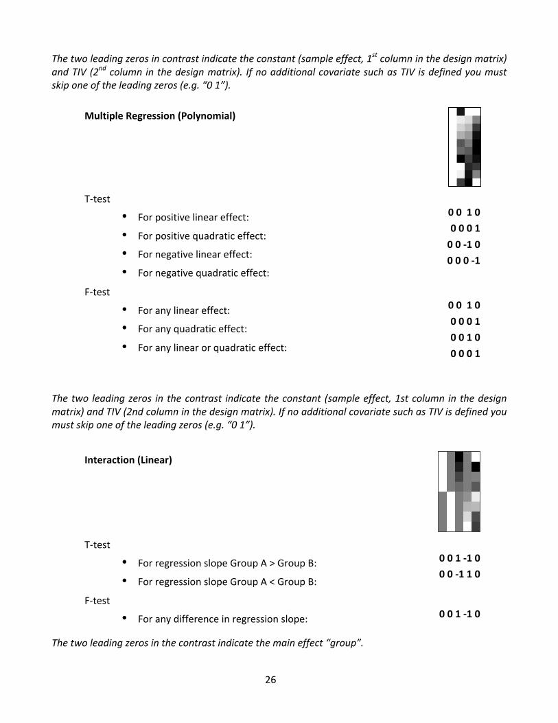
MultipleRegression(Polynomial)

T-test

• Forpositivelineareffect:

• Forpositivequadraticeffect:

• Fornegativelineareffect:

• Fornegativequadraticeffect:

0010000100-10000-1

F-test

• Foranylineareffect:

• Foranyquadraticeffect:

• Foranylinearorquadraticeffect:

0010000100100001

Thetwo leadingzeros in thecontrast indicatetheconstant (sampleeffect,1stcolumn inthedesignmatrix)andTIV(2ndcolumninthedesignmatrix).IfnoadditionalcovariatesuchasTIVisdefinedyoumustskiponeoftheleadingzeros(e.g.“01”).

Interaction(Linear)

T-test

• ForregressionslopeGroupA>GroupB:

• ForregressionslopeGroupA<GroupB:

001-1000-110

F-test

• Foranydifferenceinregressionslope:

001-10

Thetwoleadingzerosinthecontrastindicatethemaineffect“group”.

27

Interaction(Polynomial)

T-test

• ForlinearregressionslopeGroupA>GroupB:

• ForlinearregressionslopeGroupA<GroupB:

• ForquadraticregressionGroupA>GroupB:

• ForquadraticregressionGroupA<GroupB:

001-10000-110000001-10000-11

F-test

• Foranydifferenceinlinearregressionslope:

• Foranydifferenceinquadraticregression:

• Foranydifferenceinregression:

001-10000001-1001-10000001-1

Thetwoleadingzerosinthecontrastindicatethemaineffect“group”.

28

F-contrasts(effectsofinterest):IfyouwanttousetheoldSPM2F-contrast“Effectsofinterest”therespectivecontrastvectoris:

eye(n)-1/nwherenisthenumberofcolumnsofinterest.Forinteractionandregressioneffectsyouneedtoaddleadingzerosfortheconstanttermorsampleeffects:

[zeros(n,m)eye(n)-1/n]wheremisthenumberofcolumnsofnointerest.ThisF-contrastisusefultocheckifthereareanyeffectsinyourmodel(covariatesofinterest)andisneededtoplotparameterestimatesofeffectsofinterest.GettingResults:SPMmenuàResultsà[selectacontrastfromContrastManager]àDone

• MaskwithothercontrastsàNo

• Titleforcomparison:[usethepre-definednamefromtheContrastManagerorchangeit]

• Pvalueadjustmentto:o None(uncorrectedformultiplecomparisons),setthresholdto0.001o FDR(falsediscoveryrate),setthresholdto0.05,etc.o FWE(family-wiseerror),setthresholdto0.05,etc.

• Extentthreshold:(eitheruse“none”orspecifythenumberofvoxels2)

2Todeterminetheextentthresholdempirically(insteadofsaying100voxelsor500voxels,whichiscompletelyarbitrary),simplyexecuteitfirstwithoutspecifyinganextentthreshold.Thisgivesyouanoutput(i.e.,thestandardSPMglassbrainwith significant effects). If you click on “Table” (SPM main menu) you will get a table with all relevant values (MNIcoordinates,p-values,clustersizeetc.).Belowthetableyouwillfindadditionalinformation,suchas“ExpectedNumberofVoxelsperCluster”.Rememberthisnumber(thisisyourempiricallydeterminedextentthreshold).Re-runSPMàResultsetc.andenterthisnumberwhenpromptedforthe“ExtentThreshold”.Thereisalsoahiddenoptionin“CAT12àDatapresentationàThresholdandtransformspmT-maps”todefinetheextentthresholdasp-valueortousethe“ExpectedNumberofVoxelsperCluster”.

29

SpecialCases

CAT12forlongitudinaldataBACKGROUNDThemajority of VBM studies are basedon cross-sectional data inwhich one image is acquired foreach subject. However, to be able to track learning effects over time, for example, longitudinaldesignsarenecessary inwhichadditional time-pointsareacquiredforeachsubject.Theanalysisoftheselongitudinaldatarequiresacustomizedprocessing,thattakesintoaccountthecharacteristicsoftheintra-subjectanalysis.Whileimagescanbeprocessedindependentlyforeachsubjectforcross-sectionaldata,longitudinaldatamustberegisteredtothemeanimageforeachsubjectbyaninverse-consistentrealignment.Inaddition,spatialnormalizationisonlyestimatedforthemeanimageofalltimepointsandappliedtoallimages(Figure4).Additionalattentionisthenrequiredforthesetupofthe statisticalmodel. The following section therefore describes the data preprocessing andmodelsetupforlongitudinaldata.

Fig4.:FlowchartforprocessinglongitudinaldatawithCAT12.Thisfigureshowsthestepsforprocessinglongitudinaldata.Afteraninitialinverse-consistentrealignment,whichalsoincludes a bias correction between the different time points, the mean image of therealignedimagesiscalculated(mean).SpatialnormalizationparameterswiththehelpofaDartel Normalization are estimated in the next step based on the segmentations of themean image. These normalization parameters are applied to the segmentations of theimagesofalltimepoints(p1rix)andarefinallymodulated(mwp1rix).

30

Preprocessingoflongitudinaldata-overviewThe CAT12 Toolbox supplies a batch for longitudinal study design. Here, for each subject therespectiveimagesneedtobeselected.Intra-subjectrealignment,biascorrection,segmentation,andnormalizationarecalculatedautomatically.Preprocessedimagesarewrittenasmwp1r*andmwp2r*for greyandwhitematter respectively. Todefine the segmentationandnormalizationparameters,thedefaults incat_defaults.mareused.Optionallysurfacescanbeextracted inthesamewayas inthecross-sectionalpipelineandtherealignedimagesareusedforthisstep.

ComparisontoSPM12longitudinalregistrationSPM12 also offers a batch for pairwise or serial longitudinal registration. Contrary to CAT12, thismethodreliesonthedeformationsnecessarytonon-linearlyregistertheimagesofalltimepointstothemeanimage.Thesedeformationscanthenbeusedtocalculatelocalvolumechanges,whicharethenmultiplied(modulated)bythesegmentedmeanimage.However, it is not only theunderlyingmethods between SPM12 and theCAT12 longitudinal batchthat differ, but also the focus of possible applications. SPM12 additionally regularizes thedeformationswithregardtothetimedifferencesbetweentheimagesandhasitsstrengthsmoreinfinding larger effects over longer periods of time (e.g. ageing effects or atrophy). The use ofdeformationsbetweenthetimepointsmakesitpossibletoestimateanddetectlargerchanges,whilesubtleeffectsaremoredifficulttodetectovershorterperiodsoftimeintherangeofweeksorafewmonths.Incontrast,thelongitudinalpreprocessingwasdevelopedandoptimizedinCAT12todetectmoresubtleeffectsover shorterperiodsof time (e.g.brainplasticityor trainingeffectsaftera fewweeksorevenshortertimes).Unfortunately, there isnoclearrecommendationforonemethodoranother.However,oneruleofthumbcouldbetouseCAT12theshorterthetimeperiodsandthesmallertheexpectedchangesare.If you are trying to findeffects through learningor trainingor other intervention (e.g.medication,therapy) then CAT12 is the right choice. To find ageing effects or atrophy due to a(neurodegenerative)diseaseafterlongerperiodoftime,IrecommendtryingtheSPM12longitudinalregistration. For that type of data, the sensitivity of CAT12 is likely to be lower, as the DARTELregistrationisbasedonthemeanimageandisappliedtoalltimepoints. Ifthe(structural)changesbetweenthetimepointsarelarge,this is likelytoworklessreliably,althoughthishasnotyetbeensystematicallyinvestigated.Pleasenotethatthesurface-basedpreprocessing isnotaffectedbythepotentially lowersensitivityforlargerchanges,astherealignedimagesareusedindependentlytocreatethecorticalsurfacesandthickness.Thiscouldbealsoagoodalternativetofindlargerchanges.

31

OPTIONALCHANGEOFPARAMETERSFORPREPROCESSING

You can change the tissue probability map (TPM) via GUI or by changing the entry in the filecat_defaults.m(i.e. forchildrendata).AnyparametersthatcannotbechangedviatheGUImustbesetinthefilecat_defaults.m:Changeyourworkingdirectoryto“/toolbox/CAT12”inyourSPMdirectory:àselect“Utilitiesàcd”intheSPMmenuandchangetotherespectivefolder.Thenenter“opencat_defaults.m”inyourmatlabcommandwindow.Thefileisopenedintheeditor.Ifyouarenotsurehowtochangethevalues,openthemodule“SegmentData”inthebatcheditorasareference.

PREPROCESSINGOFLONGITUDINALDATA

CAT12àSegmentlongitudinaldata

Parameters:

o Data<-XàNew:SubjectàSubjectàLongitudinaldataforonesubjectàSelectFilesà[selectrawdata]àDone- Selectallvolumesforeachsubject.AstheToolboxdoesnotsupportmultispectral

data yet (i.e., different imaging methods for the same brain, such as T1-, T2-,diffusion-weighted or CT images), it is recommended to choose a T1-weightedimage.

- Select“New:Subject”toadddataforanewsubjectThedataforeachsubjectshouldbelistedasone“subject”intheBatchEditor,i.e.thereareasmanysubjectslistedasincludedintheanalysis.

àForallotheroptionsyoucanfollowtheinstructionsforpreprocessingofcross-sectionaldata as described before. Please note that not all writing options are available forlongitudinaldata.

For the naming conventions of all written files see “Naming convention of output files”. The GMsegments are mwp1r*, the WM segments are named mwp2r* if you have selected to option tomodulatethedata.Withoutmodulationtheleading“m”isomitted.

Statisticalanalysisoflongitudinaldata-overview

32

Themain interest in longitudinalstudies lies inthechangeoftissuevolumeovertimeinagroupofsubjectsorthedifferenceinthesechangesbetweentwoormoregroups.Thesetupofthestatisticalmodelneededtoevaluatethesequestions isdescribed intwoexamples.First, thecaseofonlyonegroupof4subjectswith2timepointseach(e.g.normalaging) isshown.Subsequently, thecaseoftwogroupsofsubjectsisdescribed,eachwith4timepointspersubject.Theseexamplesshouldcovermost analyses – thenumberof timepoints / groupsonly needs to be adjusted. In contrast to theanalysisofcross-sectionaldataasdescribedabove,weneedtousetheflexiblefactorialmodel,whichtakesintoaccountthatthetimepointsforeachsubjectaredependentdata.

STATISTICALANALYSISOFLONGITUDINALDATAINONEGROUP


Parameters:

o Directory<-XàSelectFilesà[selecttheworkingdirectoryforyouranalysis]àDoneo Designà“FlexibleFactorial”

§ Factorsà“New:Factor;New:Factor”Factor• Nameà[specifytext(e.g.”subject”)*]• IndependenceàYes• VarianceàEqualorUnequal• GrandmeanscalingàNo• ANCOVAàNoFactor• Nameà[specifytext(e.g.“time”)]• IndependenceàNo• VarianceàEqualorUnequal• GrandmeanscalingàNo• ANCOVAàNo

§ Specify Subjects or all Scans & Factorsà “Subjects”à “New: Subject; New:Subject;New:Subject;New:Subject;”Subject• Scansà[selectfiles(thesmoothedGMvolumesofthefirstSubject)]• Conditionsà“12”[fortwotimepoints]Subject- Scansà[selectfiles(thesmoothedGMvolumesofthesecondSubject)]- Conditionsà“12”[fortwotimepoints]Subject

*SPM is internally handling somekeyword factors such as “subject” or“repl”. If you use “subject” askeyword for the first factor theconditions can be easier defined byonlylabelingthetimepointsasinput(seebelow).

33

• Scansà[selectfiles(thesmoothedGMvolumesofthethirdSubject)]• Conditionsà“12”[fortwotimepoints]Subject- Scansà[selectfiles(thesmoothedGMvolumesofthefourthSubject)]- Conditionsà“12”[fortwotimepoints]

§ Maineffects&Interactionà“New:Maineffect”Maineffect• Factornumberà2Maineffect• Factornumberà1






STATISTICALANALYSISOFLONGITUDINALDATAINTWOGROUPS


Parameters:

o Directory<-XàSelectFilesà[selecttheworkingdirectoryforyouranalysis]àDoneo Designà“FlexibleFactorial”

§ Factorsà“New:Factor;New:Factor;New:Factor”Factor• Nameà[specifytext(e.g.”subject”)*]• IndependenceàYes• VarianceàEqual• GrandmeanscalingàNo

*SPM is internally handling somekeyword factors such as “subject” or“repl”. If you use “subject” askeyword for the first factor theconditions can be easier defined byonlylabelingthetimepointsasinput(seebelow).

34

• ANCOVAàNoFactor• Nameà[specifytext(e.g.”group”)]• IndependenceàYes• VarianceàUnequal• GrandmeanscalingàNo• ANCOVAàNoFactor• Nameà[specifytext(e.g.“time”)]• IndependenceàNo• VarianceàEqual• GrandmeanscalingàNo• ANCOVAàNo

§ Specify Subjects or all Scans & Factorsà “Subjects”à “New: Subject; New:Subject;New:Subject;New:Subject;”Subject• Scansà [select files (thesmoothedGMvolumesof the1stSubjectof first

group)]• Conditionsà“[1111;1234]’“[firstgroupwithfourtimepoints]

Donotforgettheadditionalsinglequote!Otherwiseyouhavetodefinetheconditionsas“[11;12;13;14]“

Subject• Scansà[selectfiles(thesmoothedGMvolumesofthe2ndSubjectoffirst

group)]• Conditionsà“[1111;1234]’“[firstgroupwithfourtimepoints]Subject• Scansà [select files(thesmoothedGMvolumesofthe3rdSubjectof first

group)]• Conditionsà“[1111;1234]’“[firstgroupwithfourtimepoints]Subject• Scans à [select files (the smoothed GM volumes of the 4th Subject of

secondgroup)]• Conditionsà“[2222;1234]’“[secondgroupwithfourtimepoints]Subject• Scansà[selectfiles(thesmoothedGMvolumesofthe1stSubjectofsecond

group)]• Conditionsà“[2222;1234]’“[secondgroupwithfourtimepoints]Subject

35

• Scansà [select files (the smoothed GM volumes of the 2nd Subject ofsecondgroup)]

• Conditionsà“[2222;1234]’“[secondgroupwithfourtimepoints]Subject• Scansà [select files (the smoothed GM volumes of the 3rd Subject of

secondgroup)• Conditionsà“[2222;1234]’”[secondgroupwithfourtimepoints]Subject• Scans à [select files (the smoothed GM volumes of the 4th Subject of

secondgroup)]• Conditionsà“[2222;1234]’”[secondgroupwithfourtimepoints]

§ Maineffects&Interactionà“New:Interaction;New:Maineffect”Interaction• Factornumbersà23[Interactionbetweengroupandtime]Maineffect• Factornumberà1






36

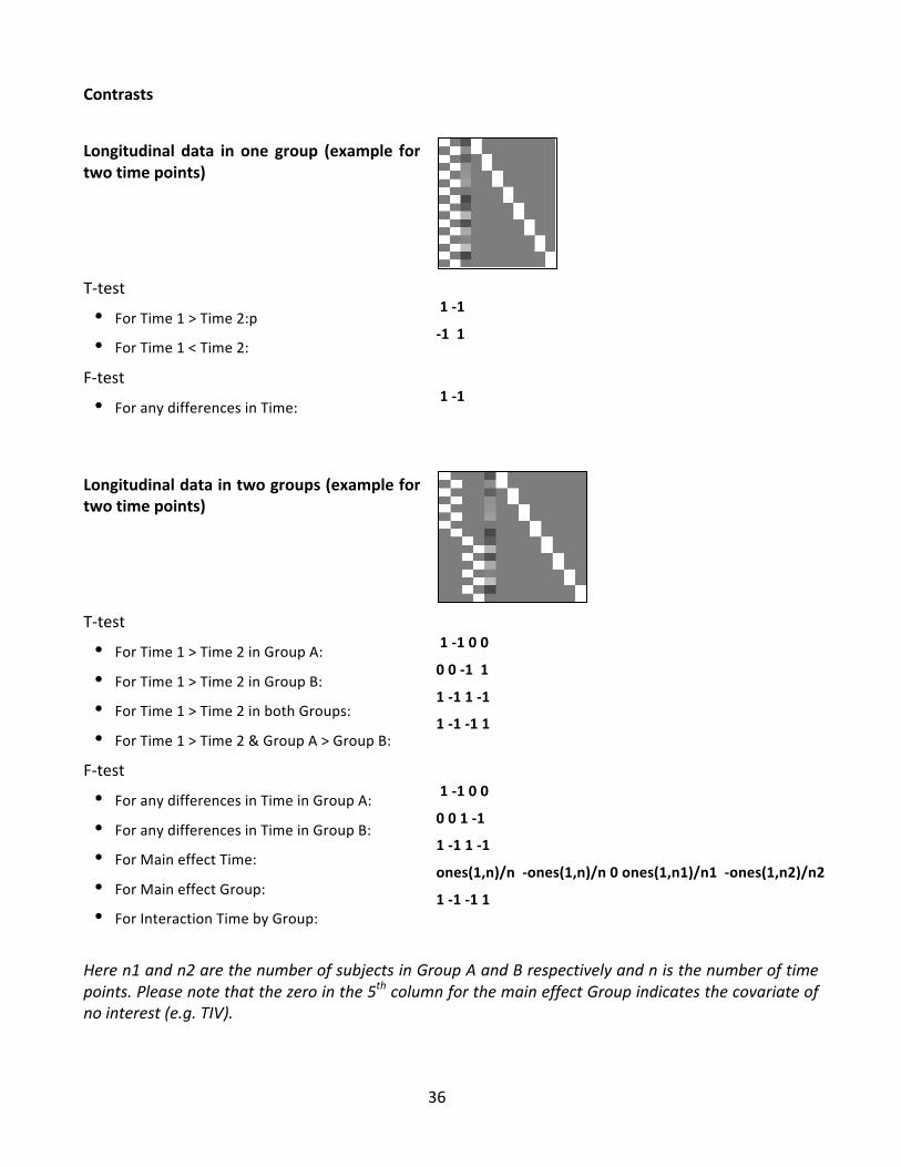
Contrasts

Longitudinal data in one group (example fortwotimepoints)

T-test

• ForTime1>Time2:p

• ForTime1<Time2:

1-1

-11

F-test

• ForanydifferencesinTime:

1-1

Longitudinaldataintwogroups(examplefortwotimepoints)

T-test

• ForTime1>Time2inGroupA:

• ForTime1>Time2inGroupB:

• ForTime1>Time2inbothGroups:

• ForTime1>Time2&GroupA>GroupB:

1-100

00-11

1-11-1

1-1-11

F-test

• ForanydifferencesinTimeinGroupA:

• ForanydifferencesinTimeinGroupB:

• ForMaineffectTime:

• ForMaineffectGroup:

• ForInteractionTimebyGroup:

1-100

001-1

1-11-1

ones(1,n)/n-ones(1,n)/n0ones(1,n1)/n1-ones(1,n2)/n2

1-1-11

Heren1andn2arethenumberofsubjectsinGroupAandBrespectivelyandnisthenumberoftimepoints.Pleasenotethatthezerointhe5thcolumnforthemaineffectGroupindicatesthecovariateofnointerest(e.g.TIV).

37

AdaptingtheworkflowsBackgroundFor most analyses, the VBM Toolbox provides all necessary tools. Since the new segmentationalgorithm is no longer dependent on Tissue Probability Maps (TPMs) and pre-defined DARTELtemplates for healthy adults exist, most questions can be evaluated using the default Toolboxsettings.However,theToolboxsettingsmaynotbeoptimalforsomespecialcases,suchasanalysisinchildrenorcertainpatientgroups.Belowwepresentstrategiesfordealingwiththesespecificcases.Customizedtissueprobabilitymaps-overviewFordataonchildrenitisagoodideatocreatecustomizedTPMs,whichreflectageandgenderofthepopulation.TheTOM8Toolbox (availablevia:https://irc.cchmc.org/software/tom.php)provides theneeded parameters to customize these TPMs. To learn more about the TOM toolbox, see alsohttp://dbm.neuro.uni-jena.de/software/tom.

CUSTOMIZEDTISSUEPROBABILITYMAPS

AbouttheTOM8Toolbox:

àselectModule“createnewtemplate”

àselect“TOM.mat”(youwillhavetodownloadthisfiletogetherwiththetoolbox)

àwritepriors/templateassinglefile

àforallothersusedefaultsettingsormodify.For“Age”eitheravectororameanage

(whenusingtheaverageapproach)mustbespecified.

ImplementationintoCAT12:

CAT12→SegmentData

Parameters:o OptionsforinitialSPM12affineregistration

§ TissueProbabilityMap(àSelectyourcustomizedTPMshere)

38

CustomizedDARTEL-template-overviewAn individual (customized) DARTEL template can be created for all cases involving at least 50-100subjects. This means that an average template of the study sample is created from the tissuesegments of the grey matter and white matter tissue segments of all subjects. Since the CAT12toolboxwritesallthefilesneededtocreatethesetemplates(“DARTELexport”),onlytwoadditionalstepsarerequired.TobeabletousethesenewlycreatedDARTEL-TemplateswiththeCAT12Toolbox,anaffineregistrationoftheDARTELexportshouldbeused.CustomizedDARTELtemplatescanthenbecreatedfromtheseaffineregisteredsegmentsandusedwiththeCAT12module“SegmentData”.

CUSTOMIZEDDARTEL-TEMPLATE

PleasenotethattheuseofyourownDARTELtemplateresultsindeviationsandunreliableresultsforROI-basedestimationsastheatlasesaredifferent.Therefore,allROIoutputsinCAT12aredisabledifyouuseyourowncustomizedDARTELtemplate.SeveralstepsarerequiredtocreatenormalizedtissuesegmentswithcustomizedDARTELTemplates.These steps canbebundledusingdependencies in theBatchEditor.The last stepcanbe repeatedwiththecustomizedtemplatesifadditionaloutputfilesarerequired.Inthefirststep,theT1imagesaresegmentedandthetissuesegmentsarenormalizedtotheTissueProbabilityMapsbymeansofanaffinetransformation.Startbyselectingthemodule“SegmentData”.CAT12àSegmentData

Parameters: àforalloptionsexcept“writingoptions”usesettingslikefora“standard”VBManalysis.

o WritingOptions

• “GreyMatter”à“Modulatednormalized”à“No”• “GreyMatter”à“DARTELexport”à“affine”• “WhiteMatter”à“Modulatednormalized”à“No”• “WhiteMatter”à“DARTELexport”à“affine”

These settings generate the volumes “rp1*-affine.nii” and “rp2*-affine.nii”, i.e. the grey (rp1) andwhite(rp2)mattersegmentsafteraffineregistration.Thefollowingmodulescanbeselecteddirectlyinthebatcheditor (SPMàToolsàDARTELToolsàRunDARTEL(createTemplates),andSPMàToolsàCAT12àCAT12:SegmentData).Itmakessensetoaddandspecifythesemodulestogetherwiththe“SegmentData”modulewithintheBatchEditorandtosetdependencies.

39

SPMàToolsàDARTELToolsàRunDARTEL(createTemplates)

Parameters:Imagesàselecttwotimes“new:Images”

§ Images:àselectthe“rp1*-affine.nii”filesorcreateadependency.§ Images:àselectthe“rp2*-affine.nii”filesorcreateadependency.

àallotheroptions:usedefaultsormodify

SPMàToolsàDARTELToolsàNormalisetoMNIspace

Parameters:DARTELTemplateàselectthefinalcreatedtemplatewiththeending“_6”.

o Selectaccordingtoà“ManySubjects”

§ Flowfields:àselectthe“u_*.nii”filesorcreateadependency.• Images: à New: Images à select the “rp1*-affine.nii” files or create a

dependency.• Images: à New: Images à select the “rp2*-affine.nii” files or create a

dependency.o Preserve:à“PreserveAmount”

o GaussianFWHM:àusedefaultsormodify

àallotheroptions:usedefaultsormodify

Please note, that a subsequent smoothing is not necessary before statistics if you have used the

option“NormalisetoMNIspace”withadefinedGaussianFWHM.

Re-useofcustomizedDARTEL-templatesOptionallyyoucanalsousethenewlycreated,customizedDARTELtemplatesintheCAT12Toolbox.

Thiscanbehelpfulifnewdataisage-wiseclosetothedatausedtocreatetheDARTELtemplate.In

thiscase,itisnotabsolutelynecessarytoalwayscreateanewtemplateandyoucansimplyusethe

previouslycreatedDARTELtemplate.Inthiscase,anadditionalregistrationtoMNI(ICBM)spacemust

beapplied:

SPMàToolsàDARTELToolsàRunDARTEL(PopulationtoICBMRegistration)

Parameters:DARTELTemplateàselectthefinalcreatedtemplatewiththeending“_6”.

40

SPMàUtilàDeformations

Parameters:Compositionà“New:DeformationField”

§ DeformationField:àselectthe“y_*2mni.nii”filefromstepabove.o Outputà“New:Pushforward”

§ Applytoàselectall“Template”fileswiththeending“_0”to“_6”.§ OutputdestinationàOutputdirectoryàselectdirectoryforsavingfiles.§ Field of Viewà Image Definedà select final “Template” file with the ending

“_6”.§ PreserveàPreserveConcentrations(no“modulation”).

Finally,thenewtemplatecanbeusedasdefaultDARTELtemplateforanynewdatathatarecloseto

thedatausedfortemplatecreation:

CAT12àSegmentData

Parameters:o Volumes<-XàSelecttheoriginalT1imageslikeinthefirstmodule“SegmentData”.

o Extended Options for CAT12 segmentationà “Spatial normalization Template”àSelectnormalizedDARTELTemplate“wTemplate*_1.nii”

- For all other options use the same settings as in the first module, ormodify.

o WritingOptionsàselecttheoutputfilesjustlikeinanystandardVBManalysis:

Please note, that now the output files have to be smoothed as usual with before the statisticalanalysis.HowtoproceedAllthestepsdescribedaboveareonlyanadaptionoftheCAT12Toolboxmodule“SegmentData”.Asalways,itisagoodideatostorethemodulesandperformaqualitycontrol.Themodules“Displayonesliceforallimages”and“Checksamplehomogeneity”fromtheCAT12Toolboxarehelpfulhere.

41

Othervariantsofcomputationalmorphometry

Deformation-basedmorphometry(DBM)BackgroundDBMisbasedontheapplicationofnon-linearregistrationprocedurestospatiallynormalizeonebraintoanotherone.Thesimplestcaseofspatialnormalizationistocorrecttheorientationandsizeofthebrain. In addition to these global changes, a non-linear normalization is necessary tominimize theremaining regional differences due to local deformations. If this local adaptation is possible, thedeformationsnowprovide informationabout the typeand localizationof thestructuraldifferencesbetweenthebrainsandcanthenbeanalyzed.Differencesbetweenthetwoimagesareminimizedandarenowcodedinthedeformations.Finally,amapoflocalvolumechangescanbequantifiedbyamathematicalpropertyofthesedeformations–the Jacobian determinant. This parameter iswell known from continuummechanics and is usuallyusedfortheanalysisofvolumechangesinflowingliquidsorgases.TheJacobiandeterminantallowsadirectestimationofthepercentagechangeinvolumeineachvoxelandcanbeanalyzedstatistically(Gaser et al. 2001). This approach is also known as tensor-basedmorphometry since the Jacobiandeterminantrepresentssuchatensor.Adeformation-basedanalysiscanbeperformednotonlyonthelocalvolumechanges,butalsoontheentire informationof thedeformations,which also includes thedirection and strengthof the localdeformations (Gaseretal.1999;2016). Sinceeachvoxel contains three-dimensional information,amultivariate statistical test is required for analysis. For this type of analysis, amultivariate generallinearmodelorHotelling’sT2testisoftenused(Gaseretal.1999;Thompsonetal.1997).AdditionalStepsinCAT12CAT12àSegmentData

Parameters:o WritingoptionsàJacobiandeterminantàNormalizedàYes

- To save the estimated volume changes change the writing option for thenormalizedJacobiandeterminantto“yes”.

ChangesinstatisticalanalysisFollow the steps for the statistical analysis as described for VBM, select the smoothed Jacobiandeterminants(e.g.swj_*.nii)andchangethefollowingparameters:CAT12→StatisticalAnalysis→BasicModels

Parameters:

o Covariates:Don’tuseTIVascovariate

42

o Masking§ ThresholdMaskingàNone§ ImplicitMaskàYes§ ExplicitMaskà../spm12/tpm/mask_ICV.nii

Surface-basedmorphometry(SBM)BackgroundSurface-based morphometry has several advantages over the sole use of volumetric data. Forexample, is has been shown that using brain surfacemeshes for spatial registration increases theaccuracy of brain registration compared to volume-based registration (Desai et al. 2005). Brainsurfacemeshesalsopermitnewformsofanalyses,suchasgyrificationindiceswhichmeasuresurfacecomplexityin3D(Yotteretal.2011b)orcorticalthickness(Gaseretal.2016).Inaddition,inflationorsphericalmappingofthecorticalsurfacemeshraisestheburiedsulcitothesurfacesothatmappedfunctionalactivityintheseregionscanbemadeeasilyvisible.LocaladaptivesegmentationGraymatter regionswith high iron concentration, such as themotor cortex and occipital regions,often have an increased intensity leading to misclassications. In addition to our adaptive MAPapproach forpartial volumesegmentation,weuseanapproach thatallows toadapt local intensitychangestodealwithvaryingtissuecontrasts(Dahnkeetal.2012a).CorticalthicknessandcentralsurfaceestimationWe use a fully automated method that allows the measurement of cortical thickness andreconstructionofthecentralsurfaceinonestep.Itusesatissuesegmentationtoestimatethewhitematter (WM)distanceandthenprojects the localmaxima (which isequal to thecortical thickness)ontoothergraymattervoxelsusinganeighboring relationshipdescribedby theWMdistance.Thisprojection-based thickness (PBT) allows the handling of partial volume information, sulcal blurring,andsulcalasymmetrieswithoutexplicitsulcusreconstruction(Dahnkeetal.2012b).TopologicalcorrectionTo repair topological defects, we use a novelmethod based on spherical harmonics (Yotter et al.2011a).Firstofall,theoriginalMRIintensityvaluesareusedtoselecteithera“fill”or“cut”operationforeachtopologicaldefect.Wemodify thesphericalmapof theuncorrectedbrainsurfacemesh insuch a way that certain triangles are preferred when searching for the bounding triangle duringreparameterization. Subsequently, a low-pass filtered alternative reconstructionbasedon sphericalharmonicsispatchedintothereconstructedsurfaceinareaswheredefectswerepreviouslypresent.SphericalmappingAsphericalmapofacorticalsurface isusuallynecessarytoreparameterizethesurfacemeshintoacommoncoordinatesystemtoenableinter-subjectanalysis.Weuseafastalgorithmtoreducearea

43

distortion,whichleadstoanimprovedreparameterizationofthecorticalsurfacemesh(Yotteretal.2011c).SphericalregistrationWe have adapted the volume-based diffeomorphic DARTEL algorithm to the surface (Ashburner,2007) toworkwith sphericalmaps (Yotteret al. 2011d).Weapply amulti-grid approach thatusesreparameterizedvaluesofsulcaldepthandshapeindexdefinedonthespheretoestimateaflowfieldthatallowsthedeformationofasphericalgrid.AdditionalStepsinCAT12CAT12àSegmentData

Parameters:o WritingoptionsàSurfaceandthicknessestimationàYes

Use projection-based thickness to estimate cortical thickness and to create thecentralcorticalsurfacefortheleftandrighthemisphere.

CAT12àSurfaceToolsàResample&SmoothSurfaces

Parameters:o SurfaceData<-XàSelectthesurfacedata(e.g.[lr]h.thickness.*)

o SmoothingFilterSizeinFWHM[usedefaultsormodify]- 12-15mmkernelsarewidelyusedforSBMandIrecommendtostartwitha

value of 15mm for thickness data and 20mm for folding data (e.g.gyrification,complexity).

o Splitjobintoseparateprocesses

- Tousemulti-threadingtheCAT12segmentationjobwithmultiplesubjectscanbe split into separateprocesses that run in thebackground.YoucanevencloseMatlab,whichwillnotaffecttheprocessesthatwillruninthebackground without GUI. If you don not want to run processes in thebackgroundthensetthisvalueto0.

- Keep in mind that each process needs about 1.5..2GB of RAM, whichshouldbeconsideredtochoosetherightnumberofprocesses.

- Please further note that no additionalmodules in the batch can be runexceptCAT12segmentation.Anydependenciesarebrokenforsubsequentmodules.

44

Extractoptionalsurfaceparameters

Youcanalsoextractadditionalsurfaceparametersthatneedtoberesampledandsmoothedwiththeabovetool.CAT12àSurfaceToolsàExtract&MapSurfaceDataàExtractAdditionalSurfaceParameters

Parameters:

o CentralSurfaces<-XàSelectthecentralsurfacedata(e.g.[lr]h.central.*)

o Gyrificationindex- Extract gyrification index (GI) based on absolute mean curvature. The

methodisdescribedinLudersetal.NeuroImage,29:1224-1230,2006.

o Corticalcomplexity(fractaldimension)ExtractCorticalcomplexity(fractaldimension)whichisdescribedinYotteretal.Neuroimage,56(3):961-973,2011.Warning:Estimationofcorticalcomplexityisveryslow!

o SulcusdepthExtractsqrt-transformedsulcusdepthbasedontheEuclideandistancebetweenthecentralsurfaceanditsconvexhull.Transformationwithsqrt-functionisusedtorenderthedatamorenormallydistributed.ChangesinstatisticalanalysisForstatisticalanalysisofsurfacemeasuresyoucanusethecommon2ndlevelmodels,whicharealsoused for VBM. Follow the steps for the statistical analysis as described for VBM and change thefollowingparameters:CAT12→StatisticalAnalysis→BasicModels

Parameters:

o Covariates:Don’tuseTIVascovariate

o Masking§ ThresholdMaskingàNone§ ImplicitMaskàYes§ ExplicitMaskà<none>

As input you have to select the resampled and smoothed files (see above). A thickness file of themerged left and right hemispheres that was resampled and smoothed with the default FWHM of15mmisnamedas: S15.mesh.thickness.resampled.name.gii

45

where“name”iftheoriginalfilenamewithoutextension.Pleasenotethatthesefilesaresavedinthesurf-folderasdefault.Donotusethe“Estimate”functionintheSPMwindow,butthecorrespondingfunctioninCAT12.ThisallowsyoutoautomaticallyoverlaytheresultsontheFreesurferaveragesurface:CAT12àStatisticalAnalysisàEstimateSurfaceModels

Regionofinterest(ROI)analysisCAT12enablestheestimationoftissuevolumes(andadditionalsurfaceparameterssuchascorticalthickness)fordifferentvolumeandsurface-basedatlasmaps(Gaseretal.2016).Alloftheseresultsareestimated inthenativespacebeforeanyspatialnormalization.Theresults foreachdatasetarestored as XML files in the label directory. The XML file catROI[s]_*.xml contains information of allatlasesasdatastructureforonedatasetandtheoptional“s” indicatessurfaceatlases.YoucanusetheCATfunction“cat_io_xml”toreadtheXMLdataasastructure.AdditionalstepsforsurfacedataWhileROI-basedvaluesforVBM(volume)dataareautomaticallystoredinthelabelfolderasXMLfileit is necessary to extract these values additionally for surface data. This must be done afterpreprocessing thedataand creating cortical surfaces. You canextractROI-basedvalues for corticalthicknessbutalsoforanyothersurfaceparameterthatextractedwiththe“ExtractAdditionalSurfaceParameters”function:CAT12àExtractROIDataàExtractROI-basedsurfacevalues

Parameters:o (Left) SurfaceData Files <-Xà Select surface data files such as lh.thickness.* for all

subjectsStatisticalanalysisofROIdataFinally,theXMLfilesofseveralsubjectscanbeanalyzedusinganexistingSPMdesignwithCAT12àAnalyzeROIs.Here,theSPM.matfileisusedtogetinformationaboutallcorrespondinglabelfiles,butalsoaboutyourdesign(includingallcovariates/confoundsyouhavemodeled).Inthisway,thesamestatistical analysis saved in the SPM.mat file is applied to your ROI data. You can then select acontrast, a threshold value and a measurement type to be analyzed (e.g. Vgm, Vwm, thickness,gyrification...) and choose between different atlas maps. The results are printed and saved asthresholdedlog-pvolumeorsurfacemap:

logPThreshold_NameOfContrast_NameOfAtlas_Measure.nii[lr]h.logPThreshold_NameOfContrast_NameOfAtlas_Measure.gii

ThesemapscanbeoptionallyvisualizedusingCAT12àDisplayResultsàSliceOverlay forvolumemapsorCAT12àDisplayResultsàDisplaysurfaceresultsforsurfacemaps.

46

Toanalyzedifferentmeasures(e.g.Vgm/Vwmforvolumesorthickness/gyrificationforsurfaces)youcan use any existing volume-based analysis to extract different volume measures, or any existingsurface-based analysis to extract different surfacemeasures. To give you an example: An existingSPM.matfilewithaVBManalysisofGMallowsyoutoanalyzeROImeasuresforboth,GMaswellasWM.Therefore,itisnotnecessarytohaveaSPM.matfileofaVBManalysisofWM.Thesameappliestosurface-basedanalysis. IfyoualreadyhaveanSPM.matfortheanalysisofcortical thickness,youcan also estimate theROI analysis for gyrificationor fractal dimension. For surfaces, however, it isnecessarytoextractROI-basedmeasuresforeachsubjectusingCAT12àExtractROIDataàExtractROI-basedsurfacevaluespriortothisstep.ForROIanalysisofsurfacesyoucanselecttheSPM.matfileoftheanalysis,eitherfortheleftorrighthemisphere,orforthemergedhemispheres.ThedesignshouldbethesameandtheROIresultsarealwaysestimatedforbothhemispheres.Pleasenotethatifyouhavemovedyourdataafterestimatingyouroriginalvoxel-orsurfaced-basedstatistics,therequiredROIfilescannotbefound.OptionalextractionofROIdataFinally,theXMLfilesofseveralsubjectscanbecombinedandsavedasCSVfileusingthe“EstimateMeanValuesinsideROI”functionforfurtheranalysis:CAT12àExtractROIDataàEstimatemeanvaluesinsideROI

Parameters:o XMLfiles<-XàSelectxmlfilesforeachsubjectthataresavedinthelabelfolder.o OutputfileàDefineoutputnameforcsvfile.Thisnameisextendedbytheatlasname

andthenameofthemeasure(e.g.“Vgm”forgraymattervolume)For eachmeasurement (e.g. “Vgm” for graymatter volume) and each atlas a separate CSV file iswritten. This works for both volume and surface data, but volume and surface data has to beprocessedseparatelywiththisfunction(surface-basedROIvaluesareindicatedbyanadditional“s”,e.g.''catROIs_'').YoucanuseexternalsoftwaresuchasExcelorSPSStoimporttheresultingCSVfilesforfurtheranalysis.Alsopayattentiontothedifferentinterpretationsbetween“.”and“,”dependingonyourregionandlanguagesettingsonyoursystem.UseofatlasfunctionsinSPM12Youcanalsousethevolume-basedatlasesdeliveredwithCATasatlasmapswithSPMatlasfunctions.ThisisparticularlyusefulifyouhaveusedthedefaultVBMprocessingpipeline,sincetheCAT12atlasmapsaretheninthesameDARTELspaceasyourdata.IfyouhaveusedthedefaultVBMprocessingpipeline, it is recommended to use CAT12 atlases in the DARTEL space instead of the SPMNeuromorphometricsatlas.TouseCAT12atlases,youmustcallthecat_install_atlasesfunctiononce,whichcopiestheatlasestoSPM.Bydefault,onlyNeuromorphometics,LPBA40,andHammersatlasmapsareused,whichareidentifiedbyaleading''dartel_''inthename.Atlasmaps for surfaces canbeusedwith the functionCAT12àDisplayResultsàDisplay SurfaceResults.Youcanuse thedatacursor function todisplayatlas regionsunder thecursor. Inaddition,

47

you canuse the ''Atlas labeling'' function to print a list of atlas regionsof the resulting clusters oroverlaytheatlasbordersonyourrenderedsurface.

Additionalinformationonnative,normalizedandmodulatedvolumesWhenpreprocessing the images (see“FirstModule:SegmentData”,onpages5-6), thedecisiononthenormalizationparametersdeterminestheinterpretationoftheanalysisresults.Pleasenotethatsomeoftheoutputoptionsareonlyavailableintheexpertmode.“Native space” creates tissue class images in spatial correspondence to theoriginaldata.Althoughthismaybeusefulforestimatingglobaltissuevolumes(e.g.GM+WM+CSF=TIV)it isnotsuitableforperforming VBM analyses due to the lack of voxel-wise correspondence in the brain). If one isinterested in these global tissue volumes in the native space (“raw values”), it is not necessary toactually output the tissue class images innative space. The “SegmentData”-function automaticallygeneratesanxml file foreachsubject (cat_*.xml),whichcontainstherawvalues forGM,WM,andCSF. The subject-specific values can be calculated (i.e., integrated into a single text file) using thefunction:CAT12àStatisticalAnalysisàEstimateTIV.“Normalized”createstissueclassimagesinspatialcorrespondencetothetemplate.ThisisusefulforVBManalyses(e.g.“concentration”ofgraymatter;Goodetal.2001;Neuroimage).“Modulatednormalized”creates tissueclass images inalignmentwith the template,butmultiplies(“modulates”)thevoxelvalueswiththeJacobiandeterminant(i.e.,linearandnon-linearcomponents)derivedfromthespatialnormalization.ThisisusefulforVBManalysesandallowsthecomparisonoftheabsoluteamountoftissue (e.g.“volume”ofgraymatter;Goodetal.2001;Neuroimage).PleasenotethatinthistypeofmodulationyoumustuseTIVascovariatetocorrectdifferentbrainsizes.Analternative approach is to use global scaling with TIV if TIV is too strongly correlated with yourcovariatesofinterest.Formoreinformation,seethesection“CheckingforDesignOrthogonality”.Ifyouusetheexpertmode,youcanoptionallychoosewhetheryouwanttomodulateyourdatafornon-lineartermsonly,whichwasthedefaultforpreviousVBM-toolboxversions.Thisproducestissueclassimagesinalignmentwiththetemplate,butthevoxelvaluesareonlymultipliedbythenon-linearcomponents.ThisisusefulforVBManalysesandallowscomparisonoftheabsoluteamountoftissuecorrected for individualbrainsizes.Thisoption issimilar tousing“Affine+non-linear” (seeabove) incombinationwith“globalnormalization”(whenbuildingthestatisticalmodelwiththetraditionalPETdesign late ons). Although this type of modulation was used in as default previous VBM-toolboxversionsitisnolongerrecommendedastheuseofstandardmodulationincombinationwithTIVascovariateprovidesmorereliableresults(Maloneetal.2015;Neuroimage).

48

NamingconventionofoutputfilesPleasenote that the resulting filesofCAT12areorganized in separate subfolders (e.g.mri, report,surf,label).Ifyoudon'twanttousesubfoldersyoucanchangetheoption"cat12.extopts.subfolders"incat_default.mto"0". Images(savedinsubfolder"mri")

SegmentedImages: #p[0123]* [m[0]w]p[0123]*[_affine].nii

Bias,noiseandintensitycorrectedT1image: #m* [w]m*.nii

Jacobiandeterminant #j_ wj_*.nii

Deformationfield(inversefield) y_(iy_) y_*.nii(iy_*.nii)

* filename

# imagespaceprefix

Imagespaceprefix:

m modulated

m0 modulatednon-linearonly(expertmodeonly)

w warped(spatiallynormalizedusingDARTEL)

Imagespaceextension:

_affine affineregisteredonly

Imagedataprefix:

p partialvolume(PV)segmentation

0 PVlabel

1 GM

2 WM

3 CSF

49

Surfacesinnativespace(savedinsubfolder"surf")

SURF.TYPE.*.gii

SURF left,righthemisphere[lh|rh]

TYPE surfacedatafile[central|sphere|thickness|gyrification|...]

central-coordinatesandfacesofthecentralsurface

sphere-coordinatesandfacesofthesphericalprojectionofthecentralsurface

sphere.reg-coordinatesandfacesofthesphereaftersphericalregistration

thickness-thicknessvaluesofthesurface

sqrtsulc-sqrt-transformedvaluesofsulculdepthbasedontheeuclideandistancebetweenthecentralsurfaceanditsconvexhull

gyrification-gyrificationvaluesbasedonabsolutemeancurvature

fractaldimension-fractaldimensionvalues(corticalcomplexity)

Surfacesin(normalized)templatespace(afterresamplingandsmoothing;savedinsubfolder"surf"bydefault)

FWHM.SURF.TYPE.RESAMP.*.gii

FWHM filtersizeinFWHMaftersmoothing(e.g.s15)

SURF left,right,orbothhemispheres[lh|rh|mesh]

TYPE surfacedatafile[thickness|gyrification|fractaldimension|...]

thickness-thicknessvaluesofthesurface

sqrtsulc - sqrt-transformed values of sulcul depth based on the euclidean distancebetweenthecentralsurfaceanditsconvexhull

gyrification-gyrificationvaluesbasedonabsolutemeancurvature

fractaldimension-fractaldimensionvalues(corticalcomplexity)

RESAMP resamplingto164k(Freesurfer)or32k(HCP)mesh[resampled|resampled_32k]

50

Imagesandsurfaceoflongitudinaldata

After processing longitudinal data, the filenames additionally contain an "r" between the originalfilenameandtheotherprefixestoindicatetheadditionalregistrationstep.Pleasealsonotethatonlythebias,noiseandintensitycorrectedaverageimageofalltimepointsforeachsubjectissaved.Reports(savedinsubfolder"report")

Global morphometric and image quality measures are stored in the cat_*.xml file. This file alsocontainsotherusefulinformationaboutsoftwareversionsandoptionsusedtopreprocessthedata.Youcanusethecat_io_xmlfunctiontoreaddatafromxml-files.Inaddition,areportforeachdatasetissavedaspdf-filecatreport_*.pdf.Regionsofinterest(ROI)data(savedinsubfolder"label")

ROIdataisoptionallysavedasxml-filecatROI[s]_*.xml.Theoptional“s”indicatessurfaceatlases.

CallingCATfromtheUNIXcommandlineYoucanalsocallCATasashellscriptfromtheUnixcommandline.Thismakesitpossibletoruntheprocess completely in the background without graphical output and distributes all given data toparalleljobs.ThiscanbeusefulifyouwanttorunCATonacomputercluster.Youcanusetheshellscriptscat_batch_cat.shorcat_batch_long.sh(forlongitudinaldata).Pleasecallthescriptsformoreinformationonhowtodefineoptionaldefaultsfiles,forexample.Thereisalsoascriptdistribute_to_server.shthatcanbeusedtodistributejobstodifferentservers.

TechnicalinformationThis toolbox is an extension of the segmentation in SPM12, but uses a completely differentsegmentationapproach.3InterpolationCAT12usesaninternalinterpolationtoprovidemorereliableresultsevenwithlowresolutionimagesand anisotropic spatial resolutions. Although interpolation cannot addmore details to the images,someofthefunctionsusedbenefitfromthehighernumberofvoxelsandtheusualstripartefactsinmodulatedimagesaregreatlyreduced.DenoisingWealsouse twonoise reductionmethods. The firstmethod is a spatial-adaptiveNon-LocalMeans(SANLM)denoisingfilterand isappliedafter intensitynormalization(Manjónetal.2010).This filter

3TheclassicSPM12segmentationisstillusedinaddition,butonlytoinitiallyremovenon-braintissuefromtheimageandtogetastartingestimateforthesegmentation.

51

removes noise while maintaining edges and is implemented as pre-processing step. The secondmethodisaclassicalMarkovRandomField(MRF)approach,whichincludesspatialinformationfromadjacent voxels in the segmentation estimation (Rajapakse et al. 1997) and is part of the AMAPsegmentation.Thestrengthofthefiltersisautomaticallydeterminedbyestimatingtheresidualnoiseintheimageorcanbesetmanually.AffinePreprocessing(APP)To improve the initial SPMsegmentation,an initialaffine registration isapplied toabias-correctedimageandthe intensityrange is limitedtoavoidproblems inspecialprotocols. If thepreprocessingfailsamoreaggressiveversionisavailablethatappliesaroughbiascorrectionandremovesnon-brainpartsthebrainbeforetheinitialaffineregistration.LocalAdaptiveSegmentation(LAS)In addition WM-inhomogeneities, GM intensity can vary for different regions such as the motorcortex, thebasalganglia,or theoccipital lobe.Thesechangeshaveananatomicalbackground (e.g.iron content, myelenization), but are dependend on the MR-protocol and often lead to GM-underestimationsathigherintensitiesandCSF-overestimationsatlowerintensities.Therefore,alocalintensitytransformationofall tissueclasses isusedtoreducetheseeffects inthe imagebeforethefinalAMAPsegmentation.ThestrengthofthechangesiscontrolledbytheLASstrparameter,with0fornoLAS,smallvalues(0.01-0.5)forsmalladjustments,0.5formediumadjustments(default),andhighervalues(0.5-1)forstrongadjustments.AMAPSegmentationThesegmentationapproachisbasedonanAdaptiveMaximumAPosterior(AMAP)techniquewithouttheneed forapriori informationon the tissueprobabilities.Thismeans that theTissueProbabilityMaps (TPM) are not constantly used in the sense of the classical Unified Segmentation approach(Ashburner et. al. 2005), but only for spatial normalization, initial skull-stripping, and as initialsegmentationestimate.ThefollowingAMAPestimationisadaptiveinthesensethatlocalvariationsof the parameters (i.e., means and variance) are modelled as slowly varying spatial functions(Rajapakseetal.1997).Thisaccountsnotonlyfor intensity inhomogeneities,butalsotoother localintensityvariations.PartialVolumeSegmentationIn addition, the segmentation approach uses a Partial Volume Estimation (PVE) with a simplifiedmixed model of a maximum of two tissue types (Tohka et al. 2004). We begin with an initialsegmentationintothreepureclasses:graymatter(GM),whitematter(WM),andcerebrospinalfluid(CSF)basedontheAMAPestimationdescribedabove.TheinitialsegmentationisfollowedbyaPVEconsistingof twoadditionalmixedclasses:GM-WMandGM-CSF.This results inanestimateof theamount(orfraction)ofeachpuretissuetypethatispresentineachvoxel(sincesinglevoxels-giventheir size - probably contain more than one tissue type) and thus allows for more precisesegmentation.

52

Skull-StrippingCAT12containsa revisedgraph-cutbased skull-stripping,with0 foramore liberal andwiderbrainmasksand1foramoreaggressiveskull-stripping.Thedefaultsettingis0.5andhasbeensuccessfullytestedonavarietyofdifferentimages.Thestrengthparameteraffectsseveralinternalparameters:

• Intensitythresholdsforthetreatmentofblood-vesselsandmeninges• Distanceandgrowthparametersforthegraph-cut/region-growing• Closingparametersthatfillthesulci• Smoothingparametersthatallowsharperorwiderresults

Ifyoursegmentationsstillcontainskullandothernon-braintissue(e.g.dura)youcantrytoincreasethestrength.Ifpartsofthebrainaremissinginthesegmentations,thestrengthcanbedecreased.CleanupCAT12includesanewcleanuproutinethatusesmorphological,distanceandsmoothingoperationstoremove the remaining meninges after the final segmentation. The strength of the cleanup iscontrolledbythecleanupstrparameter,with0fornocleanup,lowvalues<0.5forlightcleanup,0.5formediumcleanup(default),and1forstrongcleanup.SpatialNormalizationAnotherimportantextensionoftheSPM12segmentationistheintegrationoftheDARTEL(Ashburner2007)andGeodesicShooting (Ashburner&Friston2011)normalization into the toolboxbyalreadyexistingDARTELandGeodesicShootingtemplatesinMNIspace.Thesetemplateswerederivedfrom555 healthy control subjects of the IXI-database (http://www.brain-development.org) and areavailable in theMNI space4 for six different iteration steps of the DARTEL and Geodesic Shootingnormalization.Therefore,thecreationofsample-specificDARTELandGeodesicShootingtemplatesisnolongernecessaryformoststudies5.

4Therefore,noadditionalMNInormalizationisnecessary.

5Forstudiesinvestigatingchildrendata,IstillrecommendcreatingacustomizedDARTELorGeodesicShootingtemplate.However,itshouldbenotedthatthisoptionrequiresarepresentativesamplewithasufficientnumberofsubjects.

53

ReferencesJ.Ashburner(2005):Unifiedsegmentation.Neuroimage26(3):839-51.J.Ashburner(2007):Afastdiffeomorphicimageregistrationalgorithm.Neuroimage38(1):95-113.J. Ashburner (2011): Diffeomorphic registration using geodesic shooting and Gauss–Newton optimisation.Neuroimage55(3):954-967.E.Luders,P.M.Thompson,K.L.Narr,A.W.Toga,L.Jancke,C.Gaser(2006):Acurvature-basedapproachtoestimatelocalgyrificationonthecorticalsurface.Neuroimage,29(4):1224-30.C.Gaser,H.-P.Volz,S.Kiebel,S.Riehemann,H.Sauer(1999):Detectingstructuralchangesinwholebrainbasedonnonlineardeformations–applicationtoschizophreniaresearch.Neuroimage,10:107-113.C.Gaser,I.Nenadic,B.Buchsbaum,E.Hazlett,M.S.Buchsbaum(2001):Deformation-basedmorphometryanditsrelationtoconventionalvolumetryofbrainlateralventriclesinMRI.Neuroimage,13:1140-1145.C.Gaser,R.Dahnke(2016).CAT-AComputationalAnatomyToolboxfortheAnalysisofStructuralMRIData.HBM2016.http://www.neuro.uni-jena.de/hbm2016/GaserHBM2016.pdfR.Dahnke,R.Yotter,C.Gaser(2012a).Corticalthicknessandcentralsurfaceestimation.Neuroimage,65:336-348.R.Dahnke,G.Ziegler,C.Gaser(2012b).LocalAdaptiveSegmentation.HBM2012.http://www.neuro.uni-jena.de/hbm2012/HBM2012-Dahnke02.pdfR.Desai,E.Liebenthal,E.T.Possing,E.Waldron,J.R.Binder(2005):Volumetricvs.surface-basedalignmentforlocalizationofauditorycortexactivation.Neuroimage26(4):1019-29.C.D. Good, I.S. Johnsrude, J. Ashburner, R.N. Henson, K.J. Friston, R.S. Frackowiak (2001): A voxel-basedmorphometricstudyofageingin465normaladulthumanbrains.Neuroimage.14(1Pt1):21-36.I.B.Malone,K.K.Leung,S.Clegg,J.Barnes,J.L.Whitwell,J.Ashburner,N.C.Fox,G.R.Ridgway(2015):Accurateautomaticestimationoftotalintracranialvolume:anuisancevariablewithlessnuisance.Neuroimage104:366-72.J.Manjon,PCoupe,L.Marti-Bonmati,D.L.Collins,M.Robles(2010).AdaptiveNon-LocalMeansDenoisingofMRImagesWithSpatiallyVaryingNoiseLevelsJournalofMagneticResonanceImaging,31:192-203.J.C. Rajapakse, J.N. Giedd, J.L. Rapoport (1997): Statistical Approach to Segmentation of Single-ChannelCerebralMRImages.IEEETrans.Med.Imag.16(2):176-186.J. Tohka, A. Zijdenbos, A. Evans (2004): Fast and robust parameter estimation for statistical partial volumemodelsinbrainMRI.Neuroimage23(1):84-97.R.A.Yotter,R.Dahnke,P.M.Thompson,C.Gaser(2011a):TopologicalCorrectionofBrainSurfaceMeshesUsingSphericalHarmonics.HumanBrainMapping,32(7):1109-24.R.A. Yotter, G. Ziegler, I. Nenadic, P.M. Thompson,C. Gaser (2011b): Local cortical surface complexitymapsfromsphericalharmonicreconstructions.Neuroimage,56(3):961-973.R.A. Yotter, P.M. Thompson,C. Gaser (2011c): Algorithms to Improve the Re-Parameterization of SphericalMappingsofBrain.JournalofNeuroimaging,21(2):e134-47.R.A.Yotter,G.Ziegler,P.M.Thompson,C.Gaser(2011d):DiffeometricAnatomicalRegistrationontheSurface.HBM2011.

10-Apr-18 [email protected] [email protected]

Manual Computational Anatomy Toolbox - CAT12 - uni · PDF fileManual Computational Anatomy...

Documents

Transcript of Manual Computational Anatomy Toolbox - CAT12 - uni · PDF fileManual Computational Anatomy...